Searches for Interstellar HCCSH and H2CCS

Abstract

A long standing problem in astrochemistry is the inability of many current models to account for missing sulfur content. Many relatively simple species that may be good candidates to sequester sulfur have not been measured experimentally at the high spectral resolution necessary to enable radioastronomical identification. On the basis of new laboratory data, we report searches for the rotational lines in the microwave, millimeter, and sub-millimeter regions of the sulfur-containing hydrocarbon HCCSH. This simple species would appear to be a promising candidate for detection in space owing to the large dipole moment along its $b$-inertial axis, and because the bimolecular reaction between two highly abundant astronomical fragments (CCH and SH radicals) may be rapid. An inspection of multiple line surveys from the centimeter to the far-infrared toward a range of sources from dark clouds to high-mass star-forming regions, however, resulted in non-detections. An analogous search for the lowest-energy isomer, H2CCS, is presented for comparison, and also resulted in non-detections. Typical upper limits on the abundance of both species relative to hydrogen are $10^{-9}$–$10^{-10}$. We thus conclude that neither isomer is a major reservoir of interstellar sulfur in the range of environments studied. Both species may still be viable candidates for detection in other environments or at higher frequencies, providing laboratory frequencies are available.

1 Introduction

Despite being one of the most abundant elements in the interstellar medium (ISM), the sulfur content in cold molecular clouds can only account for $\sim$0.1% of that seen in warm, diffuse clouds (Tieftrunk et al., 1994; Ruffle et al., 1999), which have values comparable to the solar abundance (Bilalbegović & Baranović, 2015). To account for this “missing” sulfur, many hypotheses have been put forward regarding hidden sinks and reservoirs, including ices, dusty grains, and unknown molecular species (Martín-Doménech et al., 2016).

The search for condensed-phase sulfur has largely been unsuccessful to date. Simple molecules (such as OCS) sequestered in interstellar ice grains, for example, can only account (Boogert et al., 1997; Martín-Doménech et al., 2016) for a small amount of the total cosmic abundance ($\sim$4%). In cometary ices, the principle sulfur-bearing species appears to be H2S, with an abundance of $\sim$1.5% relative to water (Bockelée-Morvan et al., 2000), whereas FeS appears to be a major reservoir in the cometary grains themselves (Dai & Bradley, 2001). FeS grains have also been detected in protoplanetary disks, suggesting this reservoir may be widespread, and not unique to Solar System objects (Keller et al., 2002). Several recent observational and modeling studies hypothesize H2S may be a substantial sulfur reservoir in interstellar ices as well (Holdship et al., 2016; Vidal et al., 2017). While H2S is a well-known interstellar species in the gas-phase (Thaddeus et al., 1972), there has been no definitive condensed-phase observation of it outside the Solar System (Boogert et al., 2015). Recent modeling work by Laas & Caselli (2019) has shown that the sulfur depletion in cold clouds can be reproduced without the need for a significant build-up of H2S in ices, suggesting this species may play a less substantial role than previously assumed. Further investigations of condensed-phase sulfur species will undoubtedly be a strong science driver for the forthcoming James Webb Space Telescope.

New gas-phase sulfur-bearing molecules remain one of the most promising explanations for the missing sulfur content, and one that is addressable by extant radio facilities, assuming the molecules possess a permanent dipole moment and the necessary laboratory work is both available and complete (Cazzoli et al., 2016). Of the more than 200 known interstellar and circumstellar molecules, only 23 contain at least one sulfur atom (Table 1). Perhaps more striking, of the 94 molecules with five or more atoms, three contain sulfur, whereas 30 contain at least one oxygen atom (McGuire, 2018). In total, sulfur-containing species comprise $\sim$10% of the known molecular inventory of any size, whereas a third of all molecules are oxygen-containing. Despite the lower interstellar abundance of sulfur relative to oxygen (Cameron, 1973), the large disparity between the number of S- and O-bearing species is striking, and may indicate detections of large, sulfur-bearing species in space is simply limited by the lack of precise laboratory rest frequencies.

Table 1: Known interstellar and circumstellar molecules containing at least one sulfur atom and references to the first detection of those species.

Molecule	Reference
CS	Penzias et al. (1971)
SO	Gottlieb & Ball (1973)
SiS	Morris et al. (1975)
NS	Gottlieb et al. (1975); Kuiper et al. (1975)
SO+	Turner (1992)
SH+	Benz et al. (2010)
SH	Neufeld et al. (2012)
NS+	Cernicharo et al. (2018)
OCS	Jefferts et al. (1971)
H2S	Thaddeus et al. (1972)
SO2	Snyder et al. (1975)
HCS+	Thaddeus et al. (1981)
C2S	Saito et al. (1987)
S2H	Fuente et al. (2017)
HCS	Agúndez et al. (2018)
HSC	Agúndez et al. (2018)
H2CS	Sinclair et al. (1973)
HNCS	Frerking et al. (1979)
C3S	Yamamoto et al. (1987)
HSCN	Halfen et al. (2009)
CH3SH	Linke et al. (1979)
C5S	Bell et al. (1993)
CH3CH2SH	Kolesniková et al. (2014)

Large sulfur-bearing species (by interstellar standards) are perhaps improbable as substantial reservoirs of gas-phase sulfur, given the generally lower abundance of large molecules relative to simpler species (see, e.g., Belloche et al. 2013). Detailed studies of their formation chemistry, however, can provide insights into the underlying abundances (and potential reservoirs) of as-yet-undetected simpler precursor molecules. As an example, one of the most promising ways to probe formation pathways is through the study of isomeric families. Comparisons of the [H4,C2,O2] isomers glycolaldehyde, methyl formate, and acetic acid, for instance, have been used in attempts to infer branching fractions in the UV photodissociation of methanol (CH3OH), from which most of the key precursor species for the [H4,C2,O2] family are expected to form (Laas et al., 2011).

Here, we present an observational counterpart to the recent laboratory investigation of the [H2,C2,S] isomeric family of molecules. The three lowest-energy isomers in this family are H2CCS (thioketene), HCCSH (ethynethiol), and $c$-H2C2S (thiirene). The microwave and millimeter-wave spectrum of H2CCS has been previously reported by Winnewisser & Schäfer (1980), and several of the co-authors of the present work recently reported the laboratory spectrum of HCCSH from the microwave to sub-millimeter wavelengths (Lee et al., 2018). Efforts to measure the spectrum of $c$-H2C2S are currently underway. Here, we summarize the astronomical search for H2CCS and HCCSH in a number of interstellar sources spanning the evolutionary spectrum from dark clouds to high-mass star-forming regions (HMSFRs).

HCCSH would appear to be a promising candidate for astronomical detection and potential sink for sulfur for two reasons: (1) this isomer might be formed directly and efficiently via a recombination reaction involving two well-known astronomical radicals, SH and CCH (Yamada et al., 2002), and (2) HCCSH does not possess a simple, readily identifiable rotational spectrum, since the dipole moment along its $a$-inertial axis is nearly zero (0.13 D), while that along the $b$-axis is significantly larger (0.80 D). As a consequence, unlike H2CCS whose rotational spectrum is characterized by a series of lines separated in frequency by ratios of integers at low-frequency, the same lines of HCCSH are extremely faint; instead, its $b$-type lines in the millimeter- and sub-millimeter bands are much more intense [i.e., $(\mu_{b}/\mu_{a})^{2}\sim 35$].

2 Energetics and Spectroscopy

Electronic structure calculations (Lee et al., 2018) predict that the most stable isomeric arrangement of [H2,C2,S] is H2CCS, followed by HCCSH roughly 56 kJ/mol (${\sim}$6770 K) higher in energy, with the three-membered heterocycle $c$-H2C2S lying 132 kJ/mol
(${\sim}$15,900 K) above ground. Nevertheless, HCCSH can be formed by an exothermic and barrierless reaction involving SH and CCH, via reaction (R1; Lee et al. 2018):

$$\ce{SH+CCH->HCCSH}$$ (R1)

This may result in preferential production in astronomical sources in which the two radicals are prominent, although in the gas-phase it is possible that the exothermicity may result in the dissociation of a non-trivial fraction of the product, necessitating grain-surface production. The closely related [H2,C3,O] isomers provide a dramatic illustration of this effect. Although $l$-propadienone (H2CCCO) has not been observed in space despite considerable efforts (Loomis et al., 2015), isoenergetic propynal (HCCC(O)H) is prominent (Irvine et al., 1988a). Further, the considerably less stable cyclopropenone ($c$-H2C3O) has also been detected in space (Hollis et al., 2006). Taken together, these findings highlight the importance of kinetic factors in molecule formation and destruction.

Thioketene (H2CCS) has a linear heavy-atom backbone with $C_{2v}$ symmetry and ortho-para spin statistics. For this reason, it only has $a$-type rotational lines, but its dipole moment is sizable, 1.01(3) D (Winnewisser & Schäfer, 1980). At low temperature, its rotational spectrum consists of relatively closely spaced triplets that are harmonically-related spaced by $B+C$, or about 11.2 GHz. Laboratory measurements provide rest frequencies up to 230 GHz, which, given the rigidity of the molecule, can be extrapolated with reasonable confidence to better than 0.5 km s^-1 up to $\sim$450 GHz.

Although HCCSH has the same heavy atom backbone as H2CCS, owing to a different bond order along the chain, it is an asymmetric top with a bent backbone, but one still close to the prolate limit ($\kappa$ = -0.999), as defined by $\kappa$, Ray’s asymmetry parameter (Ray, 1932). A purely prolate molecule (cigar shaped, and the most common in the ISM; McGuire 2018) has $\kappa=-1$, whereas a purely oblate molecule (disk shaped) has $\kappa$ = 1. In contrast to H2CCS, HCCSH has a relatively small calculated dipole moment along its $a$-axis (0.13 D), but that along the $b$-axis (0.80 D) is significant (Lee et al., 2018). Because the $A$ rotational constant is large, 291.4 GHz, the most intense rotational lines lie at millimeter wavelengths. The detailed spectroscopic analysis of its $a$- and $b$-type transitions up to 660 GHz was presented in Lee et al. (2018).

3 Analysis

Column densities were calculated assuming a single-excitation temperature model following the formalisms of Hollis et al. (2004a) using Eq. 1 below, with corrections due to optical depth as described in Turner (1991).

$$N_{T}=\frac{1}{2}\frac{3k}{8\pi^{3}}\sqrt{\frac{\pi}{\ln 2}}\frac{Qe^{E_{u}/T_{\rm{ex}}}\Delta T_{b}\Delta V}{B\nu S_{ij}\mu^{2}}\frac{1}{1-\frac{e^{h\nu/kT_{\rm{ex}}}-1}{e^{h\nu/kT_{\rm{bg}}}-1}}$$ (1)

Here, $N_{T}$ is the total column density (cm^-2), $Q$ is the partition function, $T_{ex}$ is the excitation temperature (K), $E_{u}$ is the upper state energy (K), $\Delta T_{b}$ is the peak intensity (K), $\Delta V$ is the full-width at half-maximum of the line (km s^-1), $B$ is the beam filling factor, $\nu$ is the frequency (Hz), $S_{ij}$ is the intrinsic quantum mechanical line strength, $\mu$ is the permanent dipole moment (Debye), and $T_{bg}$ is the background continuum temperature (K). For the upper-limits presented here, a simulated spectrum was generated using the parameters described for each observation below. The strongest predicted line in the observational spectrum was then used to calculate the $1\sigma$ upper limit, taking the rms noise value at that point as the value of the brightness temperature $\Delta T_{b}$.

For HCSSH and H2CCS, we consider both the rotational partition function and the contribution from low-lying vibrational states. The total partition function is calculated according to Eq. 2,

$$Q=Q_{rot}\times Q_{vib}\times Q_{elec}$$ (2)

where $Q_{rot}$, $Q_{vib}$, and $Q_{elec}$ are the rotational, vibrational, and electronic components, respectively. Under interstellar conditions, we assume $Q_{elec}=1$. The rotational partition function was calculated via a direct summation of states as described by Gordy & Cook (1984) and Eq. 3,

$$Q_{r}=\sum_{i=0}^{\infty}(2J+1)e^{{-E_{i}}/kT_{ex}}$$ (3)

where $E_{i}$ is the energy of the $i^{th}$ rotational state. The vibrational correction was calculated according to Eq. 4,

$$Q_{\rm{vib}}=\prod\limits_{\begin{subarray}{c}i=1\end{subarray}}^{3N-6}\frac{1}{1-e^{-E_{v,i}/kT_{\rm{ex}}}}$$ (4)

where $E_{v,i}$ is the energy of the $i^{th}$ excited vibrational state. Here, we consider only the lowest five vibrational states as those higher in energy make a negligible contribution to $Q_{\rm{vib}}$.

The vibrational (harmonic) energies were calculated at the CCSD(T)/cc-pVQZ level of theory. For HCCSH, the lowest five vibrational states lie at 356, 416, 727, 848, and 942 cm^-1 above ground, while for H2CCS, they fall at 295, 352, 578, 696, and 718 cm^-1. The rotational, vibrational, and total partition functions used for the column density calculations at each temperature are listed in Tables 2 & 3 along with other molecular parameters required for the calculations.

4 Observations and Analysis

The simulated spectrum of HCCSH, with arbitrary abundance, at three different temperatures appropriate to interstellar environments (10, 80, and 200 K) is shown in Fig. 1, along with the associated observing bands of the most sensitive telescope facilities in those frequency ranges: the Robert C. Byrd 100 m Green Bank Telescope (GBT), the Atacama Large Millimeter/sub-millimeter Array (ALMA), and the GREAT instrument aboard Stratospheric Observatory for Infrared Astronomy (SOFIA). Due to its geometry, the most intense transitions fall in ALMA Bands 7 and 10 and the 1.4 THz window of the SOFIA GREAT receiver , as well as archival coverage of the Herschel HIFI instrument. Here, we examined observations from ALMA, Herschel, and the GBT targeting the HMSFRs NGC 6334I, Sgr B2(N), and Orion-KL. We also searched the line survey data toward sources from the publicly available Astrochemical Surveys at IRAM (ASAI) Large Project conducted with the IRAM 30-m telescope. The exact physical parameters assumed for each of the sources examined here are given in Tables A1 and A2.

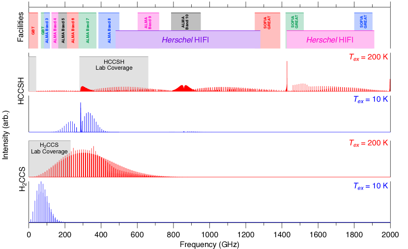
Figure 1: Simulations of HCCSH and H2CCS up to 2 THz and 1 THz, respectively, at $T_{ex}$ = 10 K (blue) and 200 K (red). The top panel of the figure shows the frequency coverage available for the GBT, ALMA, SOFIA, and in archival Herschel observations. The shaded gray regions show the extent of the frequency range that has been observed in the laboratory for these species.

4.1 NGC 6334I

NGC 6334I is a nearby HMSFR (1.3 kpc by maser parallax; Chibueze et al. 2014) with a number of embedded protostars (Hunter et al., 2006; Brogan et al., 2016; Hunter et al., 2017), young, active, and variable outflows and molecular masers (Hunter et al., 2018; Brogan et al., 2018; McGuire et al., 2018b), and a rich molecular inventory (McGuire et al., 2017). The spectra examined here toward NGC 6334I were obtained with ALMA project codes #2015.A.00022.T and #2017.1.00717.S. The spectra were extracted from (J2000) $\alpha$ = 17:20:53.374, $\delta$=-35:46:58.34. This location is nearby the MM1 embedded protostar(s), but sufficiently far from the continuum peak to minimize absorption of molecular lines.

The complete observing parameters for the Band 10 data are provided in McGuire et al. (2018b). The Band 7 observing parameters are provided in McGuire et al. (2017), with one exception. To ensure a consistent dataset, the angular resolution of the Band 7 data, originally 0.25${}^{\prime\prime}\times$0.19^′′ was degraded to match that of the Band 10 data: 0.26${}^{\prime\prime}\times$0.26^′′. The values of $T_{ex}$, $v_{lsr}$, $\Delta V$, and $T_{bg}$ for both HCCSH and H2CCS were assumed to match those described in McGuire et al. (2018b) that were found to well-reproduce the complex molecular spectra observed across both Band 7 and 10.

4.2 Orion-KL

At a distance of 414$\pm$7 pc (Menten et al., 2007), Orion-KL is perhaps the closest well-studied molecularly rich HMSFR. Indeed, six sulfur-bearing molecules were detected first toward Orion: CS, SO, H2S, SO2, HCS+, and CH3CH2SH (McGuire 2018 and refs. therein). Like NGC 6334I, it displays a complex physical structure, with a hot core, both compact and extended molecular ridges, and outflows (see Fig. 7 of Crockett et al. 2014). The spectra examined here toward Orion KL around 860 GHz are from the Herschel Observations of EXtraordinary Sources (HEXOS) key project using the Heterodyne Instrument for the Far Infrared (HIFI) instrument on the Herschel Space Observatory. The details of the observations are presented in Crockett et al. (2014). The background continuum temperature was obtained by a linear fit to the spectra prior to continuum subtraction.

For HCCSH, the values of $T_{ex}$, $v_{lsr}$, $\Delta V$, and $\theta_{s}$ were assumed to match those of HN^13CO from the analysis of Crockett et al. (2014), since this molecule is the most structurally similar one (a three heavy atom backbone with an off-axis hydrogen) to HCCSH that was not optically thick. The strongest transitions of HCCSH fall around 850 GHz (see Fig. 1), but these are both outside of the range of the laboratory measurements ($\nu_{max}$ = 660 GHz), and are of a type ($J^{\prime}_{2,K_{c}}-J^{\prime\prime}_{1,K_{c}}$) not fit by the laboratory measurements. The extrapolated frequencies are likely accurate enough to confirm a non-detection, but because of these uncertainties, we also report an upper limit derived from transitions that, while weaker, fall within the range of the laboratory measurements.

For H2CCS, we adopted the parameters from Crockett et al. (2014) for its oxygen analog H2CCO. At the assumed excitation temperature of $T_{ex}$ = 100 K, the strongest lines of H2CCS fall around 280 GHz, 200 GHz lower than the coverage of the HEXOS observations. A further reduction on the intensity of its transitions in the lowest HEXOS band occurs because of a small source size ($\theta_{s}$ = 10^′′). These factors, combined with the need to extrapolate the molecular fit substantially above the measured laboratory data, make the derived upper limit for H2CCS in this source relatively uncertain.

4.3 Sgr B2(N)

Sgr B2(N) is the premier hunting ground for new molecular detections in HMSFRs. Located at a distance of 8.3 kpc (Reid et al., 2014), this complex contains a number of embedded molecular cores separated by of order a few arcseconds (see, e.g., Bonfand et al. 2017). Molecules are typically detected in one of two regimes: either warm and compact, in the hot cores of the region (e.g., Belloche et al. 2013), or cold, diffuse, and in absorption (normally only at low frequencies), in an extended molecular shell around the region (e.g., McGuire et al. 2016). We examined three datasets for Sgr B2(N) covering a range of these conditions: the Herschel HEXOS survey at sub-millimeter wavelengths, the IRAM 30 m survey at millimeter wavelengths, and the GBT PRIMOS survey at centimeter wavelengths.

4.3.1 Herschel Data

The spectra used here toward Sgr B2(N) around 860 GHz are also from the HEXOS key project using the HIFI instrument on the Herschel Space Observatory. The details of the observations are presented in Neill et al. (2014). The background continuum temperature was obtained by a linear fit to the spectra prior to background subtraction. As with the HEXOS observations of Orion-KL, the values of $T_{ex}$, $v_{lsr}$, $\Delta V$, and $\theta_{s}$ were assumed to match those of isocyanic acid, HNCO for HCCSH, and upper limits were derived from both the strongest predicted lines, and from lines within the range of the laboratory measurements. Although substantial absorption is seen from HNCO at colder temperatures with an extended source size distribution, the warm, compact component of HN^12CO in emission is optically thin. Unlike in Orion-KL, H2CCO is not detected in Sgr B2(N), and thus we also use these same parameters derived from HNCO for H2CCS.

4.3.2 IRAM 30 m Data

At even modest excitation temperatures, the transitions of HCCSH arising in the millimeter and centimeter are too weak to provide a meaningful comparison to the limits established by the Herschel data, however, strong transitions of H2CCS are still present. A dataset at 3 mm from the IRAM 30-m telescope is available from the work of Belloche et al. (2013), and we assume for H2CCS the physical parameters derived for H2CCO from that work for the upper limit calculations.

4.3.3 GBT PRIMOS Data

Finally, if the H2CCS is particularly cold, a number of low-$J$ transitions will show bright absorption against background continuum at centimeter-wavelengths, whereas no reasonably intense signal, either in absorption or emission, can be expected for HCCSH because its transitions at these frequencies are very weak. This frequency range falls within the coverage of the Prebiotic Interstellar Molecular Survey (PRIMOS) project observations of Sgr B2(N) using the 100-m Robert C. Byrd Green Bank Telescope. Observational details and data reduction procedures are outlined in Neill et al. (2012). In the case of cold molecules observed in absorption toward Sgr B2(N), the bright background continuum against which this absorption is seen is non-thermal (Hollis et al., 2007), and has a source size of $\theta_{s}$ $\sim$20^′′ (Mehringer et al., 1993). These molecules are typically well described by a single, sub-thermal $T_{ex}$ $\sim$5 K (McGuire et al., 2016). Here, we have adopted the parameters that well-model the observed absorption signal from acetone (CH3C(O)CH3), as well as the detailed modeling of the background continuum, source size, and beam size effects, as described in the Supplementary Material of McGuire et al. (2016).

4.4 ASAI Sources

Observational details of the ASAI sources are presented in Lefloch et al. (2018); these cover a range of Solar-type protostellar sources from dark clouds to Class 0/1 protostars, including shocked outflows. Because the chemical inventories of these sources are quite varied, for the purposes of this work, we have adopted source parameters and excitation conditions for HCCSH and H2CCS representative of complex molecules previously seen in these sources, as gathered from the literature.

5 Results and Discussion

Table 2: Upper limits to HCCSH and the line parameters used to calculate them in each of the sets of observations.

Source	Frequencya	Transition	$E_{u}$	$S_{ij}\mu^{2}$	$Q$ ($Q_{rot}$, $Q_{vib}$)c	$N_{T}$	$N(\ce{H2})$	$X_{H_{2}}$	Refs.
	(MHz)	($J_{K_{a},K_{c}}^{\prime}-J_{K_{a},K_{c}}^{\prime\prime}$)	(K)	(Debye2)		(cm-2)	(cm-2)		$N(\ce{H2})$
NGC 6334I	293352.8	$16_{1,15}-16_{0,16}$	85.8	10.4	3894 (2824, 1.38)	$\leq 1.4\times 10^{16}$	–	–	–
Sgr B2(N)	618565.8	$33_{1,33}-32_{0,32}$	307.9	11.4	35808 (8441, 4.24)	$\leq 3.9\times 10^{17}$	$1\times 10^{24}$	$\leq 4\times 10^{-7}$	1
Sgr B2(N)	844982.2b	$21_{2,19}-21_{1,20}$	176.7	7.1	35808 (8441, 4.24)	$\leq 1.4\times 10^{17}$	$1\times 10^{24}$	$\leq 1\times 10^{-7}$	1
Orion-KL	618565.8	$33_{1,33}-32_{0,32}$	307.9	11.4	12664 (5442, 2.32)	$\leq 3.1\times 10^{15}$	$3.9\times 10^{23}$	$\leq 8\times 10^{-9}$	2
Orion-KL	850042.2b	$16_{2,14}-16_{1,15}$	126.6	5.3	12664 (5442, 2.32)	$\leq 3.3\times 10^{15}$	$3.9\times 10^{23}$	$\leq 8\times 10^{-9}$	2
Barnard 1	241629.5	$3_{1,3}-4_{0,4}$	16.9	1.0	57 (57, 1.00)	$\leq 2.3\times 10^{12}$	$1.5\times 10^{23}$	$\leq 2\times 10^{-11}$	3
IRAS 4A	230425.1	$4_{1,4}-5_{0,5}$	19.0	1.3	173 (173, 1.00)	$\leq 1.3\times 10^{13}$	$3.7\times 10^{23}$	$\leq 4\times 10^{-11}$	3
L1157B1	288898.1	$10_{1,9}-10_{0,10}$	42.9	6.7	855 (837, 1.02)	$\leq 5.3\times 10^{12}$	$1\times 10^{21}$	$\leq 5\times 10^{-9}$	3
L1157mm	207853.8	$6_{1,6}-7_{0,7}$	24.7	1.9	855 (837, 1.02)	$\leq 7.7\times 10^{12}$	$6\times 10^{21}$	$\leq 1\times 10^{-9}$	3
L1448R2	207853.8	$6_{1,6}-7_{0,7}$	24.7	1.9	855 (837, 1.02)	$\leq 2.1\times 10^{13}$	$3.5\times 10^{23}$	$\leq 6\times 10^{-11}$	4
L1527	162066.9	$10_{1,10}-11_{0,11}$	42.6	3.2	75 (75, 1.00)	$\leq 3.1\times 10^{12}$	$2.8\times 10^{22}$	$\leq 1\times 10^{-10}$	4
L1544	87882.4	$8_{0,8}-7_{0,7}$	19.0	0.1	57 (57, 1.00)	$\leq 1.6\times 10^{13}$	$5\times 10^{21}$	$\leq 3\times 10^{-9}$	5
SVS13A	207853.8	$6_{1,6}-7_{0,7}$	24.7	1.9	149 (149, 1.00)	$\leq 9.0\times 10^{15}$	$3\times 10^{24}$	$\leq 3\times 10^{-9}$	6
TMC1	150487.4	$11_{1,11}-12_{0,12}$	48.3	3.6	34 (34, 1.00)	$\leq 2.9\times 10^{13}$	$1\times 10^{22}$	$\leq 3\times 10^{-9}$	3

^aTypical experimental accuracy of the mm-wave measurements was $\sim$50 kHz.
^bExtrapolated beyond the upper range (660 GHz) of the laboratory measurements.
^cCalculated at the excitation temperature assumed for the source. See Table A1.
References – [1] Lis & Goldsmith 1990 [2] Crockett et al. 2014 [3] Cernicharo et al. 2018 [4] Jørgensen et al. 2002 [5] Vastel et al. 2014 [6] Chen et al. 2009

Table 3: Upper limits to H2CCS and the line parameters used to calculate them in each of the sets of observations.

Source	Frequencya	Transition	$E_{u}$	$S_{ij}\mu^{2}$	$Q$ ($Q_{rot}$, $Q_{vib}$)f	$N_{T}$	$N(\ce{H2})$	$X_{H_{2}}$	Refs.
	(MHz)	($J_{K_{a},K_{c}}^{\prime}-J_{K_{a},K_{c}}^{\prime\prime}$)	(K)	(Debye2)		(cm-2)	(cm-2)		$N(\ce{H2})$
NGC 6334I	292685.4b	$26_{1,25}-25_{1,24}$	203.2	78.2	9051 (5456, 1.66)	$\leq 4.7\times 10^{15}$	–	–	–
Sgr B2(N)c	22407.9	$2_{0,2}-1_{0,1}$	1.6	2.0	31 (31, 1.00)	$\leq 6.4\times 10^{12}$	$1\times 10^{24}$	$\leq 6\times 10^{-12}$	1
Sgr B2(N)d	100828.5	$9_{0,9}-8_{0,8}$	24.2	9.0	12106 (6395, 1.89)	$\leq 2.9\times 10^{16}$	$1\times 10^{24}$	$\leq 3\times 10^{-8}$	1
Sgr B2(N)e	494982.4b	$44_{1,43}-43_{1,42}$	548.3	132.5	121982 (16448, 7.42)	$\leq 2.7\times 10^{17}$	$1\times 10^{24}$	$\leq 3\times 10^{-7}$	1
Orion-KL	494982.4b	$44_{1,43}-43_{1,42}$	548.3	132.5	4410 (3466, 1.27)	$\leq 3.2\times 10^{15}$	$3.9\times 10^{23}$	$\leq 8\times 10^{-9}$	2
Barnard 1	89626.7	$8_{0,8}-7_{0,7}$	19.4	8.2	104 (104, 1.00)	$\leq 5.0\times 10^{11}$	$1.5\times 10^{23}$	$\leq 3\times 10^{-12}$	3
IRAS 4A	89626.7	$8_{0,8}-7_{0,7}$	19.4	8.2	334 (334, 1.00)	$\leq 2.5\times 10^{12}$	$3.7\times 10^{23}$	$\leq 7\times 10^{-12}$	3
L1157B1	213921.0	$19_{1,18}-18_{1,17}$	116.2	58.0	1725 (1648, 1.05)	$\leq 3.1\times 10^{12}$	$1\times 10^{21}$	$\leq 3\times 10^{-9}$	3
L1157mm	211738.3	$19_{1,19}-18_{1,18}$	115.1	58.0	1725 (1648, 1.05)	$\leq 2.4\times 10^{12}$	$6\times 10^{21}$	$\leq 4\times 10^{-10}$	3
L1448R2	100311.4	$9_{1,9}-8_{1,8}$	37.6	27.2	1725 (1648, 1.05)	$\leq 4.2\times 10^{12}$	$3.5\times 10^{23}$	$\leq 1\times 10^{-11}$	4
L1527	78825.9	$7_{1,6}-6_{1,5}$	28.6	21.0	139 (139, 1.00)	$\leq 3.1\times 10^{11}$	$2.8\times 10^{22}$	$\leq 1\times 10^{-11}$	4
L1544	89626.7	$8_{0,8}-7_{0,7}$	19.4	8.2	104 (104, 1.00)	$\leq 2.2\times 10^{11}$	$5\times 10^{21}$	$\leq 4\times 10^{-11}$	5
SVS13A	100828.5	$9_{0,9}-8_{0,8}$	24.2	9.2	286 (286, 1.00)	$\leq 9.1\times 10^{15}$	$3\times 10^{24}$	$\leq 3\times 10^{-9}$	6
TMC1	134430.3	$12_{0,12}-11_{0,11}$	41.9	12.2	57 (57, 1.00)	$\leq 5.5\times 10^{12}$	$1\times 10^{22}$	$\leq 6\times 10^{-10}$	3

^aWithin the range of the measurements (60–230 GHz), Winnewisser & Schäfer 1980 claim a typical accuracy of $\sim$16.5 kHz.
^bExtrapolated beyond the upper range (230 GHz) of the laboratory measurements.
^cGBT (PRIMOS) Observations.
^dIRAM 30-m Observations.
^eHerschel HIFI Observations.
^fCalculated at the excitation temperature assumed for the source. See Table A2.
References – [1] Lis & Goldsmith 1990 [2] Crockett et al. 2014 [3] Cernicharo et al. 2018 [4] Jørgensen et al. 2002 [5] Vastel et al. 2014 [6] Chen et al. 2009

In addition to the formation of HCCSH via reaction (R1), as proposed by Lee et al. (2018), several additional reaction pathways would appear at least qualitatively plausible. For example, both quantum chemical (Ochsenfeld et al., 1999) and laboratory work (Galland et al., 2001) have shown that HCS/HSC can be readily produced by a reaction involving atomic carbon:

$$\ce{H2S+C->HCS/HSC+H}.$$ (R2)

It is not unreasonable, therefore, to speculate that HCS/HSC could further react with atomic carbon, followed by hydrogenation, to yield both HCCSH and H2CCS on grain surfaces. Indeed, successive hydrogenation reactions beginning from CS or C2S could also yield HCS/HSC intermediates, or perhaps even HCCSH and H2CCS directly (see, e.g., Lamberts 2018). Further quantum chemical and laboratory work exploring the efficiency, branching ratios, and rates of these reactions would certainly help to shed light on the viability of these pathways.

It is also important to consider the potential destruction pathways of these species as well, and in this context it may be enlightening to compare the [H2,C2,S] species with a similar family of isomers having the formula [H2,C3,O]. As mentioned earlier, one rather longstanding astronomical mystery has been why the most stable of these isomers, propadienone (H2CCCO) has thus far remained undetected in space (Loomis et al., 2015; Loison et al., 2016), despite detections of two higher-energy forms, propynal (HCCCHO) and cyclopropenone ($c$-H2C3O) (Irvine et al., 1988a; Hollis et al., 2006), there. Recently, an ab initio study involving reactions between atomic hydrogen and propadienone and propynal revealed unexpectedly that only the addition to propadienone, i.e.

$$\ce{H+H2CCCO->H2CCHCO,}$$ (R3)

was barrierless and exothermic (Shingledecker et al., 2019). Moreover, it was found that the radical formed via (R3) could again subsequently react with H to form propenal (CH2CHCHO), a species which in fact has been observed by Hollis et al. (2004b) in Sgr B2(N), where the other isomers of [H2,C3,O] have been detected. Thus, reaction (R3) likely keeps the abundance of propadienone low, both on grains – where it serves as a precursor to propenal – and in the gas, where the association product likely dissociates.

Similarly, given the high mobility of atomic hydrogen on grain surfaces – particularly in warm environments – it may be the case that H2CCS and/or HCCSH are efficiently destroyed by H. Intriguingly, the detection of the related saturated species CH3CH2SH in Orion-KL by Kolesniková et al. (2014) hints at the successive hydrogenation of a CCS backbone, with either of the linear [H2,C2,S] isomers potentially serving as precursors. Detailed calculations of these types of reactions could therefore reveal whether such kinetic effects might play a role in explaining the observational results described here.

Given that the structurally analogous H2CCC, H2CCN, and H2CCO are all known interstellar species (Cernicharo et al., 1991; Irvine et al., 1988b; Turner, 1977), the non-detections of both HCCSH and H2CCS is somewhat surprising. In a few cases, there are hints of emission at appropriate frequencies, but nevertheless, no signal was seen that could be even tentatively assigned with any confidence to either HCCSH or H2CCS. Upper limits to the column densities were established for each molecule in each source and are summarized in Tables 2 and 3, along with the pertinent line parameters. The observational spectra around each transition used to calculate the upper limits, as well as a simulation of the molecular spectra using those upper limits, are shown in Figures B1 and B2.

Given the large number of non-detections presented here, we conclude that neither H2CCS nor HCCSH are substantial interstellar sulfur reservoirs. These species, along with $c$-H2C2S, however, remain reasonable candidates for interstellar detection in sensitive observations, but probably in a source very rich in sulfur-bearing species. We note that the upper limits reported here could be substantially improved if additional laboratory spectroscopy is performed. As shown in Fig. 1, the laboratory data for both HCCSH and H2CCS fail to cover the strongest transitions of these species in warm environments. In sources where line confusion is not an issue, the errors introduced by extrapolation would likely not preclude detection, but would instead require additional observing time owing to the need for wider frequency coverage. In line-confused sources, however, such as NGC 6334I in ALMA Band 10, frequency extrapolation can not be made with confidence, making any purported detection highly tenuous. Similarly, while the strong $b$-type branch of HCCSH near 1.4 THz is likely to be identifiable with SOFIA even if the frequencies are slightly uncertain, the search space would be substantially narrowed by laboratory measurements in this band. Finally, a search for the higher-energy cyclic isomer, c-H2C2S, is currently impossible due to the lack of any laboratory spectra.

6 Conclusions

A search for HCCSH and H2CCS in a number of astronomical line surveys based on newly-reported laboratory rest-frequencies obtained with a combination of microwave and sub-millimeter spectroscopy is presented. Non-detections are reported in all sources, suggesting that these molecules are not substantial reservoirs of sulfur, nor can they be readily used to infer sulfur chemistry. A possible explanation for the absence of HCCSH is an analogous destruction pathway to l-propadienone by barrierless, exothermic reaction with atomic hydrogen in the solid state. The detection of the strongest transitions of HCCSH, which arise at THz frequencies, remains a possibility, and would be substantially aided by additional enabling laboratory work.

Appendix A Source Parameters

The physical parameters assumed for each source examined here are provided in Tables A1 and A2.

Table A1: Source parameters assumed for HCCSH in each of the sets of observations.

Source	Telescope	$\theta_{s}^{a}$	$T_{bg}$	$\Delta V$	$T_{b}^{\dagger}$	$T_{ex}$	Refs.	Notes
		(′′)	(K)	(km s-1)	(mK)	(K)
NGC 6334I	ALMA	–	28.2	3.2	16.0b	135	1
Sgr B2(N)	Herschel	2.3	7.1	8.0	81.8	280	2	At 619 GHz
Sgr B2(N)	Herschel	2.3	10.9	8.0	77.0	280	2	At 845 GHz
Orion-KL	Herschel	10	5.5	6.5	27.5	209	3	At 619 GHz
Orion-KL	Herschel	10	8.7	6.5	78.0	209	3	At 850 GHz
Barnard 1	IRAM	–	2.7	0.8	12.1	10	4, 5
IRAS 4A	IRAM	–	2.7	5.0	10.3	21	4, 6
L1157B1	IRAM	–	2.7	8.0	4.4	60	7
L1157mm	IRAM	–	2.7	3.0	4.7	60	7
L1448R2	IRAM	–	2.7	8.0	4.7	60	8
L1527	IRAM	–	2.7	0.5	6.8	12	8, 9
L1544	IRAM	–	2.7	0.5	2.9	10	10, 11
SVS13A	IRAM	0.3	2.7	3.0	7.8	80	4, 6
TMC1	IRAM	–	2.7	0.3	7.6	7	12, 13

^aExcept where noted, the source is assumed to fill the beam.

^bFor these interferometric observations, the intensity is given in mJy/beam rather than mK.

^†Taken either as the 1$\sigma$ RMS noise level at the location of the target line, or for line confusion limited spectra, the reported RMS noise of the observations.

References – [1] McGuire et al. 2018b [2] Neill et al. 2014 [3] Crockett et al. 2014 [4] Melosso et al. 2018 [5] Cernicharo et al. 2018 [6] Higuchi et al. 2018 [7] McGuire et al. 2015 [8]Jørgensen et al. 2002 [9] Araki et al. (2017) [10] Hily-Blant et al. 2018 [11] Crapsi et al. 2005 [12] McGuire et al. 2018a [13] Gratier et al. 2016

Table A2: Source parameters assumed for H2CCS in each of the sets of observations.

Source	Telescope	$\theta_{s}^{a}$	$T_{bg}$	$\Delta V$	$T_{b}^{\dagger}$	$T_{ex}$	Refs.
		(′′)	(K)	(km s-1)	(mK)	(K)
NGC 6334I	ALMA	–	28.2	3.2	2.0b	135	1
Sgr B2(N)	GBT	20	28.4	12.0	-4.5	5	14
Sgr B2(N)	IRAM	2.2	5.2	7.0	12.0	150	15
Sgr B2(N)	Herschel	2.3	5.1	8.0	42.1	280	2
Orion-KL	Herschel	10	4.3	3.0	20.0	100	3
Barnard 1	IRAM	–	2.7	0.8	2.9	10	4, 5
IRAS 4A	IRAM	–	2.7	5.0	2.4	21	4, 6
L1157B1	IRAM	–	2.7	8.0	2.4	60	7
L1157mm	IRAM	–	2.7	3.0	4.9	60	7
L1448R2	IRAM	–	2.7	8.0	2.6	60	8
L1527	IRAM	–	2.7	0.5	3.5	12	8, 9
L1544	IRAM	–	2.7	0.5	2.0	10	10, 11
SVS13A	IRAM	0.3	2.7	3.0	2.2	80	4, 6
TMC1	IRAM	–	2.7	0.3	6.6	7	12, 13

^aExcept where noted, the source is assumed to fill the beam.

^bFor these interferometric observations, the intensity is given in mJy/beam rather than mK.

^†Taken either as the 1$\sigma$ RMS noise level at the location of the target line, or for line confusion limited spectra, the reported RMS noise of the observations.

References – [1] McGuire et al. 2018b [2] Neill et al. 2014 [3] Crockett et al. 2014 [4] Melosso et al. 2018 [5] Cernicharo et al. 2018 [6] Higuchi et al. 2018 [7] McGuire et al. 2015 [8]Jørgensen et al. 2002 [9] Araki et al. (2017) [10] Hily-Blant et al. 2018 [11] Crapsi et al. 2005 [12] McGuire et al. 2018a [13] Gratier et al. 2016 [14] Neill et al. 2012 [15] Belloche et al. 2013

Appendix B Non-Detection Figures

Figures B1 and B2 show the transition used to calculate the upper limit in each source, simulated using the upper limit column density and parameters given in Tables 2, 3, A1, and A2.

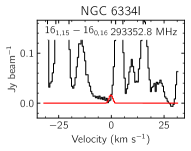
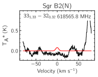
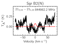
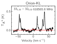
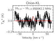
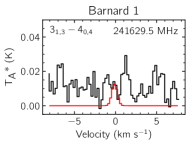
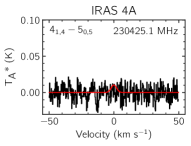
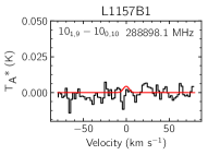
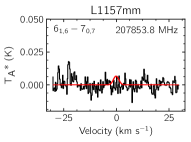
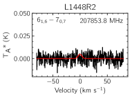
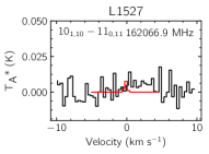
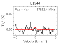
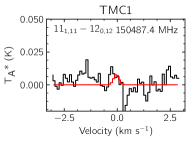
Figure B1: Transitions of HCCSH used to calculate the upper limits given in Table 2. In each panel, the red trace shows the transition simulated using the derived upper limit column density and the physical parameters assumed for that source. The frequency of the transition is given in the upper right of each panel, and the quantum numbers for each transition in the upper left. The source name is given above each panel. Due to the large variances between observations, the intensity and velocity axes are not uniform between each panel.

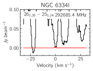
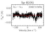
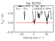
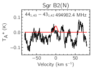
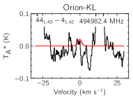
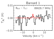
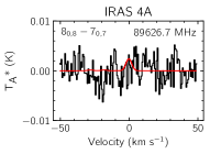
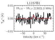
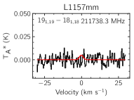
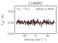
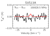
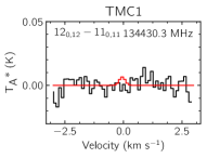
Figure B2: Transitions of H2CCS used to calculate the upper limits given in Table 3. In each panel, the red trace shows the transition simulated using the derived upper limit column density and the physical parameters assumed for that source. The frequency of the transition is given in the upper right of each panel, and the quantum numbers for each transition in the upper left. The source name is given above each panel. Due to the large variances between observations, the intensity and velocity axes are not uniform between each panel.

References

- Agúndez et al. (2018) Agúndez, M., Marcelino, N., Cernicharo, J., & Tafalla, M. 2018, A&A, 611, L1
- Araki et al. (2017) Araki, M., Takano, S., Sakai, N., et al. 2017, ApJ, 847, 0
- Bell et al. (1993) Bell, M. B., Avery, L. W., & Feldman, P. A. 1993, ApJ, 417, L37
- Belloche et al. (2013) Belloche, A., Müller, H. S. P., Menten, K. M., Schilke, P., & Comito, C. 2013, A&A, 559, A47
- Benz et al. (2010) Benz, A. O., Bruderer, S., van Dishoeck, E. F., et al. 2010, A&A, 521, L35
- Bilalbegović & Baranović (2015) Bilalbegović, G., & Baranović, G. 2015, MNRAS, 446, 3118
- Bockelée-Morvan et al. (2000) Bockelée-Morvan, D., Lis, D. C., Wink, J. E., et al. 2000, A&A, 353, 1101
- Bonfand et al. (2017) Bonfand, M., Belloche, A., Menten, K. M., Garrod, R. T., & Müller, H. S. P. 2017, A&A, 604, A60
- Boogert et al. (2015) Boogert, A. C. A., Gerakines, P. A., & Whittet, D. C. B. 2015, ARA&A, 53, 541
- Boogert et al. (1997) Boogert, A. C. A., Schutte, W. A., Helmich, F. P., Tielens, A. G. G. M., & Wooden, D. H. 1997, A&A, 317, 929
- Brogan et al. (2016) Brogan, C. L., Hunter, T. R., Cyganowski, C. J., et al. 2016, ApJ, 832, 187
- Brogan et al. (2018) —. 2018, ApJ, 866, 87
- Cameron (1973) Cameron, A. G. W. 1973, Space Sci. Rev., 15, 121
- Cazzoli et al. (2016) Cazzoli, G., Lattanzi, V., Kirsch, T., et al. 2016, A&A, 591, A126
- Cernicharo et al. (1991) Cernicharo, J., Gottlieb, C. A., Guélin, M., et al. 1991, ApJ, 368, L39
- Cernicharo et al. (2018) Cernicharo, J., Lefloch, B., Agúndez, M., et al. 2018, ApJ, 853, L22
- Chen et al. (2009) Chen, X., Launhardt, R., & Henning, T. 2009, ApJ, 691, 1729
- Chibueze et al. (2014) Chibueze, J. O., Omodaka, T., Handa, T., et al. 2014, ApJ, 784, 114
- Crapsi et al. (2005) Crapsi, A., Caselli, P., Walmsley, C. M., et al. 2005, ApJ, 619, 379
- Crockett et al. (2014) Crockett, N. R., Bergin, E. A., Neill, J. L., et al. 2014, ApJ, 787, 112
- Dai & Bradley (2001) Dai, Z. R., & Bradley, J. P. 2001, Geochimica et Cosmochimica Acta, 65, 3601
- Frerking et al. (1979) Frerking, M. A., Linke, R. A., & Thaddeus, P. 1979, ApJ, 234, L143
- Fuente et al. (2017) Fuente, A., Goicoechea, J. R., Pety, J., et al. 2017, ApJ, 851, L49
- Galland et al. (2001) Galland, N., Caralp, F., Rayez, M.-T., et al. 2001, The Journal of Physical Chemistry A, 105, 9893
- Gordy & Cook (1984) Gordy, W., & Cook, R. L. 1984, Microwave Molecular Spectra, 3rd edn. (New York: Wiley)
- Gottlieb & Ball (1973) Gottlieb, C. A., & Ball, J. A. 1973, ApJ, 184, L59
- Gottlieb et al. (1975) Gottlieb, C. A., Ball, J. A., Gottlieb, E. W., Lada, C. J., & Penfield, H. 1975, ApJ, 200, L147
- Gratier et al. (2016) Gratier, P., Majumdar, L., Ohishi, M., et al. 2016, ApJS, 225, 1
- Halfen et al. (2009) Halfen, D. T., Ziurys, L. M., Brünken, S., et al. 2009, ApJ, 702, L124
- Higuchi et al. (2018) Higuchi, A. E., Sakai, N., Watanabe, Y., et al. 2018, ApJS, 236, 0
- Hily-Blant et al. (2018) Hily-Blant, P., Faure, A., Vastel, C., et al. 2018, MNRAS, 480, 1174
- Holdship et al. (2016) Holdship, J., Viti, S., Jimenez-Serra, I., et al. 2016, MNRAS, 463, 802
- Hollis et al. (2004a) Hollis, J. M., Jewell, P. R., Lovas, F. J., & Remijan, A. 2004a, ApJ, 613, L45
- Hollis et al. (2004b) Hollis, J. M., Jewell, P. R., Lovas, F. J., Remijan, A., & Møllendal, H. 2004b, ApJ, 610, L21
- Hollis et al. (2007) Hollis, J. M., Jewell, P. R., Remijan, A. J., & Lovas, F. J. 2007, ApJ, 660, L125
- Hollis et al. (2006) Hollis, J. M., Remijan, A. J., Jewell, P. R., & Lovas, F. J. 2006, ApJ, 642, 933
- Hunter et al. (2006) Hunter, T. R., Brogan, C. L., Megeath, S. T., et al. 2006, ApJ, 649, 888
- Hunter et al. (2017) Hunter, T. R., Brogan, C. L., MacLeod, G., et al. 2017, ApJ, 837, L29
- Hunter et al. (2018) Hunter, T. R., Brogan, C. L., MacLeod, G. C., et al. 2018, ApJ, 854, 0
- Irvine et al. (1988a) Irvine, W. M., Brown, R. D., Cragg, D. M., et al. 1988a, ApJ, 335, L89
- Irvine et al. (1988b) Irvine, W. M., Friberg, P., Hjalmarson, Å., et al. 1988b, ApJ, 334, L107
- Jefferts et al. (1971) Jefferts, K. B., Penzias, A. A., Wilson, R. W., & Solomon, P. M. 1971, ApJ, 168, L111
- Jørgensen et al. (2002) Jørgensen, J. K., Schöier, F. L., & van Dishoeck, E. F. 2002, A&A, 389, 908
- Keller et al. (2002) Keller, L. P., Hony, S., Bradley, J. P., et al. 2002, Nature, 417, 148
- Kolesniková et al. (2014) Kolesniková, L., Tercero, B., Cernicharo, J., et al. 2014, ApJ, 784, L7
- Kuiper et al. (1975) Kuiper, T. B. H., Kakar, R. K., Kuiper, E. N. R., & Zuckerman, B. 1975, ApJ, 200, L151
- Laas & Caselli (2019) Laas, J. C., & Caselli, P. 2019, A&A, 624, A108
- Laas et al. (2011) Laas, J. C., Garrod, R. T., Herbst, E., & Widicus Weaver, S. L. 2011, ApJ, 728, 71
- Lamberts (2018) Lamberts, T. 2018, A&A, 615, L2
- Lee et al. (2018) Lee, K. L. K., Martin-Drumel, M.-A., Lattanzi, V., et al. 2018, Molecular Physics, 6, in press
- Lefloch et al. (2018) Lefloch, B., Bachiller, R., Ceccarelli, C., et al. 2018, MNRAS, 477, 4792
- Linke et al. (1979) Linke, R. A., Frerking, M. A., & Thaddeus, P. 1979, ApJ, 234, L139
- Lis & Goldsmith (1990) Lis, D. C., & Goldsmith, P. F. 1990, ApJ, 356, 195
- Loison et al. (2016) Loison, J.-C., Agúndez, M., Marcelino, N., et al. 2016, MNRAS, 456, 4101
- Loomis et al. (2015) Loomis, R. A., McGuire, B. A., Shingledecker, C., et al. 2015, ApJ, 799, 34
- Martín-Doménech et al. (2016) Martín-Doménech, R., Jimenez-Serra, I., Muñoz Caro, G. M., et al. 2016, A&A, 585, A112
- McGuire (2018) McGuire, B. A. 2018, ApJS, 239, 17
- McGuire et al. (2018a) McGuire, B. A., Burkhardt, A. M., Kalenskii, S. V., et al. 2018a, Science, 359, 202
- McGuire et al. (2016) McGuire, B. A., Carroll, P. B., Loomis, R. A., et al. 2016, Science, 352, 1449
- McGuire et al. (2015) McGuire, B. A., Carroll, P. B., Dollhopf, N. M., et al. 2015, ApJ, 812, 1
- McGuire et al. (2017) McGuire, B. A., Shingledecker, C. N., Willis, E. R., et al. 2017, ApJ, 851, L46
- McGuire et al. (2018b) McGuire, B. A., Brogan, C. L., Hunter, T. R., et al. 2018b, ApJ, 863, L35
- Mehringer et al. (1993) Mehringer, D. M., Palmer, P., Goss, W. M., & Yusef-Zadeh, F. 1993, ApJ, 412, 684
- Melosso et al. (2018) Melosso, M., Melli, A., Puzzarini, C., et al. 2018, A&A, 609, A121
- Menten et al. (2007) Menten, K. M., Reid, M. J., Forbrich, J., & Brunthaler, A. 2007, A&A, 474, 515
- Morris et al. (1975) Morris, M., Gilmore, W., Palmer, P., Turner, B. E., & Zuckerman, B. 1975, ApJ, 199, L47
- Neill et al. (2012) Neill, J. L., Muckle, M. T., Zaleski, D. P., et al. 2012, ApJ, 755, 153
- Neill et al. (2014) Neill, J. L., Bergin, E. A., Lis, D. C., et al. 2014, ApJ, 789, 8
- Neufeld et al. (2012) Neufeld, D. A., Falgarone, E., Gerin, M., et al. 2012, A&A, 542, L6
- Ochsenfeld et al. (1999) Ochsenfeld, C., Kaiser, R. I., Lee, Y. T., & Head-Gordon, M. 1999, The Journal of Chemical Physics, 110, 9982
- Penzias et al. (1971) Penzias, A. A., Solomon, P. M., Wilson, R. W., & Jefferts, K. B. 1971, ApJ, 168, L53
- Ray (1932) Ray, B. S. 1932, Zeitschrift für Physik, 78, 74
- Reid et al. (2014) Reid, M. J., Menten, K. M., Brunthaler, A., et al. 2014, ApJ, 783, 130
- Ruffle et al. (1999) Ruffle, D. P., Hartquist, T. W., Caselli, P., & Williams, D. A. 1999, MNRAS, 306, 691
- Saito et al. (1987) Saito, S., Kawaguchi, K., Yamamoto, S., et al. 1987, ApJ, 317, L115
- Shingledecker et al. (2019) Shingledecker, C. N., Álvarez-Barcia, S., Korn, V. H., & Kästner, J. 2019, ApJ, 878, 0
- Sinclair et al. (1973) Sinclair, M. W., Fourikis, N., Ribes, J. C., et al. 1973, Australian Journal of Physics, 26, 85
- Snyder et al. (1975) Snyder, L. E., Hollis, J. M., Ulich, B. L., et al. 1975, ApJ, 198, L81
- Thaddeus et al. (1981) Thaddeus, P., Guélin, M., & Linke, R. A. 1981, ApJ, 246, L41
- Thaddeus et al. (1972) Thaddeus, P., Kutner, M. L., Penzias, A. A., Wilson, R. W., & Jefferts, K. B. 1972, ApJ, 176, L73
- Tieftrunk et al. (1994) Tieftrunk, A., Pineau des Forêts, G., Schilke, P., & Walmsley, C. M. 1994, A&A, 289, 579
- Turner (1977) Turner, B. E. 1977, ApJ, 213, L75
- Turner (1991) —. 1991, ApJS, 76, 617
- Turner (1992) —. 1992, ApJ, 396, L107
- Vastel et al. (2014) Vastel, C., Ceccarelli, C., Lefloch, B., & Bachiller, R. 2014, ApJ, 795, L2
- Vidal et al. (2017) Vidal, T. H. G., Loison, J.-C., Jaziri, A. Y., et al. 2017, MNRAS, 469, 435
- Winnewisser & Schäfer (1980) Winnewisser, M., & Schäfer, E. 1980, Zeitschrift für Naturforschung A, 35
- Yamada et al. (2002) Yamada, M., Osamura, Y., & Kaiser, R. I. 2002, A&A, 395, 1031
- Yamamoto et al. (1987) Yamamoto, S., Saito, S., Kawaguchi, K., et al. 1987, ApJ, 317, L119