Two-dimensional disordered Mott metal-insulator transition

Abstract

We studied several aspects of the Mott metal-insulator transition in the disordered case. The model on which we based our analysis is the disordered Hubbard model, which is the simplest model capable of capturing the Mott metal-insulator transition. We investigated this model through Statistical Dynamical Mean-Field Theory (statDMFT). This theory is a natural extension of Dynamical Mean-Field Theory (DMFT), which has been used with relative success in the last several years with the purpose of describing the Mott transition in the clean case. As is the case for the latter theory, statDMFT incorporates the electronic correlation effects only in their local manifestations. Disorder, on the other hand, is treated in such a way as to incorporate Anderson localization effects. With this technique, we analyzed the disordered two-dimensional Mott transition, using Quantum Monte Carlo to solve the associated single-impurity problems. We found spinodal lines at which the metal and insulator cease to be meta-stable. We also studied spatial fluctuations of local quantities, such as self-energy and local Green’s function, and showed the appearance of metallic regions within the insulator and vice-versa. We carried out an analysis of finite-size effects and showed that, in agreement with the theorems of Imry and Ma, the first-order transition is smeared in the thermodynamic limit. We analyzed transport properties by means of a mapping to a random classical resistor network and calculated both the average current and its distribution across the metal-insulator transition.

I Introduction

A phase transition at $T=0$ as a function of some external parameter is called a quantum phase transition. It is characterized by a singular change in the ground state of the system. Although zero temperature is impossible to achieve, the effects of this quantum phase transition at $T=0$ are felt at finite temperatures. Hence the importance of studying these transitions. A quantum phase transition of great importance is the metal-insulator transition. The distinction between metallic and insulating behavior is only well defined at zero temperature: while the resistivity of an insulator diverges as $T\rightarrow 0$, this transport property approaches a constant value in the case of a metal. At finite temperatures, the resistivity is finite in both cases. As a result, one could imagine that the metal-insulator transition is necessary a quantum phase transition. However, several systems exhibit an abrupt jump of resistivity, by several orders of magnitude, at finite temperature. It is therefore natural to extend the concept of the metal-insulator transition to the case of finite temperatures. The metal-insulator transition has been observed in several physical systems such as (i) doped semiconductor systems (e.g. Si:P,B (Rosenbaum et al., 1983; M. A. Paalanen, 1991)), (ii) two-dimensional electron systems in MOSFETs (“metal-oxide-semiconductor field-effect transistors” (Anissimova et al., 2007)) and semiconductor heterostructures (GaAs/AlGaAs) (Hanein et al., 1998; Lilly et al., 2003), (iii) transition metal compounds ($\textrm{V}_{2}\textrm{O}_{3},\textrm{V}\textrm{O}_{2},\textrm{NiSSe},\textrm{Nb}$)(Lederer et al., 1972; J. Mazzaferro, 1980), and (iv) organic conductors, e.g. $\kappa-(\textrm{BETD TTF})_{2}\textrm{Cu}[(\textrm{N}(\textrm{CN})_{2}]\textrm{Cl}$)(Limelette et al., 2003). Many of these systems are not pure, displaying intrinsic or extrinsic disorder.

State-of-the-art imaging techniques have enabled researchers to investigate systems undergoing metal-insulator transitions with nanoscale resolution (Liu et al., 2017). This has opened a new window into the transport properties of disordered strongly correlated systems. Thus, it has become clear that beneath the total resistance of a sample, the usual indicator of the metal-insulator transition, lurks in fact an intricate inhomogeneous landscape. Indeed, in many cases, the insulating behavior appears as poorly conducting puddles nucleate and grow within the metallic host and vice-versa. The first observation of this phenomenon was made in VO₂ films on sapphire substrate by means of scattering near-field infrared scanning spectroscopy (Qazilbash et al., 2007, 2009). Stripy puddles were also observed in microcrystals of the same system O’Callahan et al. (2015) as well as in films (Liu et al., 2013) with a unidirectional substrate induced strain, revealing that the electronic degrees of freedom are strongly coupled to the lattice ones. These studies reveal that such non-uniform state is induced by various inhomogeneities such as defects, strains, surfaces, cracks, etc. It is clear that a theoretical descriptions incorporating these features in a strongly correlated setting is called for. This is what we propose to do in the present work.

There are some known mechanisms capable of transforming a metal into an insulator. In the absence of interactions, a sufficiently large level of disorder leads to the localization of the wave functions of a particle, the so-called Anderson localization (P.W.Anderson, 1958). A great deal is known about this mechanism. In particular, a successful scaling theory (Abrahams et al., 1979) has shown that all states of a particle are localized in the presence of any level of disorder in dimensions $d\leq 2$ (considering only the case of potential scattering, ignoring the cases of potentials with spin-orbit interaction). When $d>2$, you must add a minimal amount of disorder for the metal to become an insulator. This transition is known as the Anderson metal-insulator transition. Alternatively, Mott proposed that, even in the absence of disorder, the electron-electron interactions may in some circumstances induce a metal-insulator transition (Mott, 1990). Although the original Mott mechanism was essentially based on the long-term character of the Coulomb interaction, a model with interactions of short range proposed by Hubbard (Hubbard, 1963, 1964a, 1964b) can also exhibit a metal-insulator transition for sufficiently strong electronic interactions when there is one electron per site of the crystal lattice. Because of these initial proposals, this transition induced by the interactions is known as the Mott or Mott-Hubbard transition. The problem of understanding the conjunction of disorder and interactions (Lee and Ramakrishnan, 1985; Altshuler and Aronov, 1979; Castellani et al., 1984, 1987), despite some progress, is still an essentially open problem.

Theoretically, several techniques have been developed to describe the Mott transition. One of the first was made by Hubbard himself in a series of works (Hubbard, 1963, 1964a, 1964b). His approach consists essentially in starting with the limit in which the electron-electron interaction is much larger than the kinetic energy of the system (the insulator), and gradually reducing the value of this interaction. The characteristic gap of the Mott insulator, separating two bands of excitations called Hubbard bands, finally closes at a critical value of the interaction $U=U_{cHubb}$ and the system is metalized. An opposite point of view is due to Brinkman and Rice (Brinkman and Rice, 1970). Using a variational wave function proposed by Gutzwiller (Gutzwiller, 1963, 1964, 1965), they analyzed how the correlated metal is destroyed by the increase of electronic interactions. In this case, at a certain critical value of the interaction $U=U_{cBR}$, the strongly correlated quasi-particles of the Fermi liquid disappear and the system becomes an insulator. While Hubbard’s description does not adequately describe the quasi-particles of the correlated metal, the Brinkman and Rice approach cannot correctly predict the presence of the Hubbard bands. Both characteristics can be observed, for example, in optical conductivity measurements, which indicate the incompleteness of these two approaches.

The advent of the Dynamical Mean-Field Theory (DMFT) (Metzner and Vollhardt, 1989; Georges et al., 1996) enabled a description of the Mott transition that unifies the views of Hubbard and Brinkman-Rice. DMFT is able to incorporate, for intermediate values of the interaction $U$, both the quasi-particles of the Fermi liquid at low energies and the incoherent Hubbard bands at high energies. In this description, the Mott transition is a first order transition, characterized by the disappearance of the quasi-particles and leaving behind only the finite energy excitations of the Hubbard bands. The transition is characterized by the existence of a region of coexistence between the metallic and the insulating phases, as in the case of supercooling and superheating in the liquid-gas transition. Also as in the case of that transition, the first-order phase transition line in the temperature $T$ versus the interaction $U$ phase diagram ends at a second-order critical point at ($T_{c}$, $U_{c}$). Below $T_{c}$, the resistivity exhibits a jump as a function of $U$. This jump decreases with increasing temperature and disappears at the critical point.

The disordered Hubbard model was studied previously with several methods: exact diagonalization (Kotlyar and Das Sarma, 2001), finite- (Ulmke and Scalettar, 1997; Denteneer et al., 1999; Paris et al., 2007) and zero-temperature (Srinivasan et al., 2003; Chang and Scalettar, 2012) quantum Monte Carlo techniques, Hartree-Fock (Heidarian and Trivedi, 2004; Shinaoka and Imada, 2009, 2010), variational wave functions (Pezzoli and Becca, 2010), DMFT (Ulmke et al., 1995; Tanasković et al., 2003; Aguiar et al., 2005; Andrade et al., 2009) and typical medium theory (Dobrosavljevic et al., 2003; Byczuk et al., 2005, 2009; Dobrosavljevic, 2010; Sen et al., 2016, 2018). We should mention also the related problem of the disordered Coulomb liquid (Benenti et al., 1999; Punnoose and Finkel’stein, 2005). All of these approaches, with their strengths and weaknesses, focus on different aspects and shed some light on this difficult problem, yet no final picture has emerged.

In the present work, we employ an extension of the DMFT picture of the Mott transition that is able to incorporate non-trivial disorder effects, the so-called Statistical Dynamical Mean Field Theory (statDMFT) (Dobrosavljevic and Kotliar, 1997). The most important features of this method are (i) the incorporation of all Anderson localization effects (in fact, the method is exact in the non-interacting limit), which affects the properties of single-particle states and (ii) the incorporation of local interaction effects, such as in the original DMFT. Non-local interaction effects are absent in this approach. We therefore used this method to study the effects of disorder on the Mott transition in a two-dimensional lattice model with randomness. As in the DMFT, a method is required for the solution of the auxiliary single-impurity problems. We used Quantum Monte Carlo (the Hirsch-Fye algorithm (Hirsch and Fye., 1986)) to solve this single-impurity problems. Related DMFT approaches to other types of non-homogeneous systems have been also used in diverse contexts (Potthoff and Nolting, 1999; Miller and Freericks, 2001; Freericks, 2004; Okamoto and Millis, 2005; Chen and Freericks, 2007; Florens, 2007; Snoek et al., 2008; Helmes et al., 2008a, b; Gorelik et al., 2010; Byczuk et al., 2019).

Our results show that adding disorder to the system keeps the first-order character of the transition for finite-sized systems, including the coexistence of both metallic and insulating solutions, although the position of the transition fluctuates spatially. The average hysteresis loops, however, are shifted to larger values of the interaction. Furthermore, for a given disorder realization, we observe how increasing (reducing) the electron-electron interaction in a metallic (insulating) system induces the the nucleation and growth of insulating (metallic) “bubbles”, in striking similarity to the near-field imaging results on VO₂. As expected for a two-dimensional system, however, as the system size increases, there is a proliferation of both metallic and insulating “bubbles”, signaling the smearing of the first-order transition in the thermodynamic limit. Finally, we show how we can employ a classical random-resistor model to describe the transport on a microscopic level, thus offering a means to analyze these highly complex inhomogeneous states.

II The model

We focus on the site-disordered Hubbard model in a two-dimensional square lattice with first and second nearest-neighbor hopping, as defined by the Hamiltonian:

$$H = H_{0}+H_{W}+H_{U},$$ (1)

where

$$H_{0} = -\underset{\left\langle i,j\right\rangle\sigma}{\sum}t\left(c_{i\sigma}^{\dagger}c_{j\sigma}+\mathrm{h.c.}\right)$$ (2)

$$-\underset{\left\langle\left\langle i,j\right\rangle\right\rangle\sigma}{\sum}\left(t^{*}c_{i\sigma}^{\dagger}c_{j\sigma}+\mathrm{h.c.}\right),$$

$$H_{W} = \underset{i\sigma}{\sum}\epsilon_{i}n_{i\sigma},$$ (3)

and

$$H_{U} = U\underset{i}{\sum}\left(n_{i\uparrow}-\frac{1}{2}\right)\left(n_{i\downarrow}-\frac{1}{2}\right).$$ (4)

Here, $c_{i\sigma}^{\dagger}$ creates an electron with spin projection $\sigma$ at site $i$ and $n_{i\sigma}=c_{i\sigma}^{\dagger}c_{i\sigma}$ is the number operator. The lattice parameter is set to $a=1$ and a purely imaginary second nearest-neighbor hopping $t^{*}$ is introduced in order to move the van Hove singularity away from middle of the clean non-interacting band while at the same time maintaining particle-hole symmetry. We will fix it to be $t^{*}=0.5it$. The particle-hole symmetric Hubbard $U$ term accounts for a local Coulomb repulsion. Particle-hole symmetry is destroyed only by the diagonal disorder term $\epsilon_{j}$ which is distributed according to a uniform probability distribution of total width $W$ centered at zero, which can be taken as a measure of disorder strength. The clean non-interacting dispersion relation is $\epsilon_{k}=-2t\left(\cos k_{x}+\cos k_{y}+\sin k_{x}\sin k_{y}\right)$ and the corresponding density of state is shown in Fig. 1. The half band width is $D=\frac{\sqrt{2}+1}{2}t\approx 1.207t$, which we will take as our energy unit.

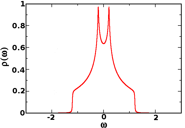
Figure 1: The clean non-interacting density of states of our model. Note that the van Hove singularities occur away from the band center.

III The statistical Dynamical Mean Field Theory (statDMFT)

The spirit of single-site dynamical mean field theory and its descendants is to treat exactly on-site correlations. This is achieved by assuming a local albeit frequency-dependent self-energy. In the context of a disordered lattice, this amounts to the following approximation to the full self-energy

$$\mathbf{\mathbf{\Sigma}}_{ij}(i\omega_{n})\rightarrow\delta_{ij}\mathbf{\mathbf{\Sigma}}_{i}(i\omega_{n}),$$ (5)

here written in its Matsubara version. Note that, although local, the self-energy $\mathbf{\mathbf{\Sigma}}_{i}(i\omega_{n})$ varies from site to site. The self-energy is calculated within a self-consistent scheme as follows. Under the assumption of Eq. (5), the local dynamics of a generic site i is governed by the effective action

$$\begin{array}[]{ccc}S_{eff}^{(i)}&=&-\underset{\sigma}{\sum}\iint c_{i\sigma}^{\dagger}(\tau)g_{0}^{(i)-1}(\tau-\tau^{\prime})c_{i\sigma}(\tau^{\prime})d\tau d\tau^{\prime}\\ &+&U\int\left[n_{i\uparrow}(\tau)-\frac{1}{2}\right]\left[n_{i\downarrow}(\tau)-\frac{1}{2}\right]d\tau,\end{array}$$ (6)

where

$$g_{0}^{(i)-1}(i\omega_{n})=i\omega_{n}-\epsilon_{i}-\triangle_{i}(i\omega_{n}),$$ (7)

and $\Delta_{i}(i\omega_{n})$ is the “cavity” function describing single-particle hopping to and from site $i$. The local interacting Green’s function, obtained by solving the effective action in Eq. (6) and defined by

$$G_{i}(\tau-\tau^{\prime})=-\left\langle T\left[c_{i\sigma}(\tau)c_{i\sigma}^{\dagger}(\tau^{\prime})\right]\right\rangle,$$ (8)

is related to the self-energy through

$$G_{i}^{-1}(i\omega_{n}) = g_{0}^{(i)-1}(i\omega_{n})-\mathbf{\mathbf{\Sigma}}_{i}(i\omega_{n}).$$ (9)

From the set of equations Eq.(6)-Eq.(9) an iterative calculational scheme can be devised. Given a finite $L\times L$ realization of the disordered lattice, we start from an initial guess for the $L^{2}$ “cavity” functions $\Delta_{i}(i\omega_{n})$, which define $L^{2}$ effective actions as given by Eq.(6) and Eq.(7). We then use some standard impurity solver to calculate the $L^{2}$ local interacting Green’s functions from Eq.(8) and then find the $L^{2}$ local self-energies from Eq.(9). This ensemble of local self-energies now has to be used to generate updated “cavity” functions. This is achieved by focusing on the single-particle lattice Green’s function, which can be easily written as a resolvent in the lattice site basis (matrices in this basis are denoted by a hat)

$$\widehat{G}_{lat}(i\omega_{n})=\frac{1}{i\omega_{n}\widehat{1}-\widehat{H}_{0}-\widehat{H}_{W}-\widehat{\mathbf{\Sigma}}(i\omega_{n})},$$ (10)

where $\widehat{1}$ is the unitary matrix and $\widehat{\mathbf{\Sigma}}(i\omega_{n})$ is the diagonal matrix with elements $\mathbf{\Sigma}_{i}(i\omega_{n})\delta_{i,j}$. Physically, the renormalization introduced by interactions are encoded in a “shift” of the site energies by a frequency-dependent self-energy

$$\epsilon_{i}\rightarrow\epsilon_{i}+\mathbf{\Sigma}_{i}(i\omega_{n}).$$ (11)

As usual in single-site DMFT-based approaches, this renormalization only describes local, single-particle processes. The lattice Green’s function $\widehat{G}_{lat}(i\omega_{n})$ of Eq. (10) is obtained by a frequency-by-frequency numerical inversion of the non-Hermitian operator in the denominator. The latter can be efficiently implemented in the site basis and the numerical inversion performed with standard linear algebra routines. In the site basis, the diagonal elements of $\widehat{G}_{lat}(i\omega_{n})$ are the updated local Green’s functions $G_{i}^{\left(new\right)}(i\omega_{n})$ of Eq. (9). Therefore, the updated “cavity” functions can be obtained from

$$\Delta_{i}^{\left(new\right)}(i\omega_{n})=i\omega-\epsilon_{i}-G_{i}^{\left(new\right)-1}(i\omega_{n})-\mathbf{\mathbf{\Sigma}}_{i}(i\omega_{n}),$$ (12)

which is then used to generate a new set of $L^{2}$ effective actions, thus closing self-consistency loop. The full self-consistent scheme has been dubbed statistical dynamical mean field theory (statDMFT). The great advantage of the method lies in its ability to track full distributions (typically numerically) of local quantities, instead of focusing on average, either algebraic (as in the infinite-dimensional DFMT limit) or geometric (as in the “typical medium theory”) (Dobrosavljevic et al., 2003; Byczuk et al., 2005, 2009; Dobrosavljevic, 2010; Sen et al., 2016, 2018). Evidently, when interactions are turned off, the method represents the exact diagonalization of the non-interacting disordered problem.

It should be mentioned that originally the DMFT of clean systems was introduced by invoking its exactness in the infinite-dimensional limit Metzner and Vollhardt (1989). Indeed, the infinite coordination suppresses fluctuations in the same way as in the mean-field treatment of spin systems. DMFT’s subsequent popularization and widespread use in finite-dimensional systems, however, has come from the realization that many strongly correlated systems are well described within a local treatment of correlations. In this sense, DMFT and its descendants represent the optimal implementation of this local program. This has become especially clear in the description of the clean Mott-Hubbard transition end-point Limelette et al. (2003). Of course, other low-temperature instabilities (like magnetism) are especially sensitive to a finite, low dimensionality. Thus, our use of the method in a two-dimensional case can be justified in two ways: (a) we work close to the second-order end-point of the clean transition, and (b) most of our focus is on the particularity of two spatial dimensions, where the Imry-Ma effect destroys the clean first-order transition line, as will be explained later.

We have implemented the statDMFT approach to study the disordered Mott transition in the two-dimensional Hubbard model at half filling. We have focused on three different temperatures with the following choice of parameters: $T=0.028D$ , $T=0.024D$ and $T=0.02D$ and the value of disorder was fixed at $W=0.52D$. Since we focus on finite temperatures, the issue of antiferromagnetic order, which only occurs at $T=0$ in two dimensions is not important here. In our calculations, we have used the Quantum Monte Carlo algorithm of Hirsch and Fye (Hirsch and Fye., 1986) as impurity solver. The discretization of the imaginary time axis was set at $\triangle\tau$=0.55. At each run of the impurity solver, the number of sweeps used to obtain the converged results was $100,000$. The number of iterations needed to reach the full self-consistency of the statDMFT equations was less than $50$ for well-defined metallic or insulating solutions, but increased closer to the critical points, where it could range from $200$ to $500$ interactions.

IV The Mott-Hubbard phase transition and the effects of disorder

Theoretical and experimental studies indicate that the Mott transition belongs to the same universality class of the liquid-gas phase transition and the Ising model(Kotliar et al., 2000). The clean Hubbard model Hamiltonian in the presence of a chemical potential reads

$$\begin{array}[]{ccc}H&=&H_{0}+H_{U}-\underset{i\sigma}{\sum}\mu n_{i\sigma}\end{array}.$$ (13)

For values of the local interaction $U>U_{c}$, the system displays insulating behavior when the mean occupancy number $\left\langle n\right\rangle=1$. For values of $\left\langle n\right\rangle\neq 1$, the system is metallic. The phase diagram of the transition corresponds to a first order transition at $n=1$, culminating at a second-order critical point at $T_{c}$, as shown in Fig. 2. This figure also shows the dependence of $n$ on the chemical potential $\mu$ for $T=0$. Note that there is a plateau at $n=1$, since the presence of the Mott gap makes the system incompressible $(dn/d\mu=0)$. We would like to emphasize that this phase diagram stands in complete analogy with the phase diagram of the Ising model in an external (longitudinal) field $h$ when we make the correspondences $\left(n-1\right)\to m$ (where $m$ is the magnetization density) and $\mu\to h$.

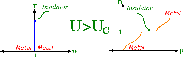
Figure 2: $T-n$ phase diagram for the Mott transition and occupation number as a function of chemical potential at $T=0$ in the Hubbard model.

Based on the above behavior, it is clear that the diagonal disorder $H_{W}=\underset{i\sigma}{\sum}\epsilon_{i}n_{i\sigma}$ act as a “local” chemical potential by doping the insulator and making it metallic in a given region for sufficiently large values of $\left|\epsilon_{i}\right|$. By analogous reasoning to the Ising model with random fields (See and e. g, 1997), if the fluctuations of $\left|\epsilon_{i}\right|$ are sufficiently large in a certain region, the insulator is unstable with respect to the formation of a metallic region . If $N$ is the number of sites within the region, then the fluctuations are such that

$${\color[rgb]{1,0,0}{\color[rgb]{0,0,0}\triangle\epsilon}} = \sqrt{\frac{\underset{i}{\sum\epsilon_{i}^{2}}}{N-1}}\left\{\begin{array}[]{cc}{\color[rgb]{1,0,0}{\color[rgb]{0,0,0}\lesssim\triangle\epsilon_{c}}}&\mathtt{{\color[rgb]{0,0,1}{\color[rgb]{0,0,0}Remains\>Insulating,}}}\\ {\color[rgb]{1,0,0}{\color[rgb]{0,0,0}\gtrsim\triangle\epsilon_{c}}}&\mathtt{{\color[rgb]{0,0,1}{\color[rgb]{0,0,0}Local\>Metallization,}}}\end{array}\right.$$ (16)

where $\triangle\epsilon_{c}\sim U$ when $T=0$. Therefore, the region remains insulating if the size of fluctuations is less than a critical value, above which we have local metallization. This is analogous to the effect of the random field on the Ising model. We should mention that a careful scaling analysis of the near-field imaging results of Qazilbash et al., 2007 gave strong support to a picture of the metal-insulator transition in VO₂ based on the random field Ising model universality class (Liu et al., 2016; See and e. g, 1997).

There is a crucial dimension dependence to this phenomenon, however. Indeed, the same considerations as used by Imry and Ma (Imry and Ma, 1975) in their analysis of the random field Ising model lead us to conclude that disorder destroys the two-dimensional Metal-Insulator transition in the thermodynamic limit. This is because below and at two dimensions the interface energy between metal and insulator is not able to hinder the proliferation of metallic regions in the insulator or insulating regions in the metal. Therefore, the system breaks into various metal and insulating regions and the phase transition is smeared. The first-order phase transition line on the left-hand side of Fig. 2 is destroyed in this two-dimensional case. This is the generalization of the Imry and Ma theorem (Imry and Ma, 1975) to the Mott transition case.

Finally, we need to explain how we determine whether a certain region belongs to an insulating or a metallic “bubble”. The local density of states (DOS) might be a good indicator. In a clean system, it can be obtained through the value of the local Green’s function at a particular value of the imaginary time (Trivedi and Randeria, 1995)

$$G_{i}\left[\tau=\frac{1}{2k_{B}T}\right].$$ (17)

This approach, however, assumes that the local DOS does not vary appreciably with the frequency on the scale of the temperature. This is a reasonable assumption in a clean Hubbard model, in which the only energy scales are $U$ and $D$. In a disordered Hubbard model, however, the local on-site energies fluctuate in the range $\left[-W/2,W/2\right]$, thus generating a continuum of small energy scales over which the local DOS varies and invalidating this procedure. Another option would be the local self-energy at low real frequencies, since

$$\mathrm{Re}\Sigma_{i}\left(\omega\right)\to\begin{cases}0&\mathrm{metal},\\ \infty&\mathrm{insulator}.\end{cases}$$ (18)

This indicator would require the analytical continuation from Matsubara to real frequencies, a notably difficult task. Since this must be performed at every lattice site, we tried to create an automated algorithm to do this, using the usual maximum entropy and Padé techniques. However, this proved to be very unreliable. In the end, we opted for the value of the imaginary part of the local self-energy at the first Matsubara frequency $\mathrm{Im}\Sigma_{i}\left(i\omega_{1}\right)$, since it reflects the same tendency of Eq. (18), being large in the insulator and small in the metal

$$\mathrm{Im}\Sigma(i\omega_{1})\sim\left\{\begin{array}[]{cc}i\omega_{1}\to 0\ \mathrm{as}\ T\to 0&\mathrm{metal},\\ 1/i\omega_{1}\to 0\ \mathrm{as}\ T\to 0&\mathrm{insulator}.\end{array}\right.$$ (19)

V Transport properties

It would be useful to use the data from $\mathrm{Im}\Sigma_{i}(i\omega_{1})$ as a means to access the transport properties within statDMFT. This is possible at $T=0$ in the non-interacting case by means of the Landauer formalism (Landauer, 1970), through the calculation of the transmission matrix between the edges of the system. This formalism was later extended to interacting systems and finite temperatures Meir and Wingreen (1992) enabling a full statDMFT calculation of transport properties. Nonetheless, when the transport occurs without quantum coherence at any length scale due to the strong inelastic scattering, it is possible to make a classical description of the resistivity. We will show that at the temperatures and interactions in which we work, transport is completely incoherent and we will thus use a network of classical resistors to calculate the relative resistance values of the system. To our knowledge, this is the first attempt to calculate transport within statDMFT, albeit in this incoherent regime.

From many-body theory, there is a relation between the value of self-energy at zero (real) frequency and wave vector on the Fermi surface and the inelastic half-life of the particle (Fetter and Walecka, 1970)

$$\mathrm{Im}\Sigma(\left|\vec{k}\right|\sim k_{F},\omega\simeq 0)\sim\frac{1}{\tau_{in}\left(\vec{k}\right)}.$$ (20)

If $\tau_{in}(\vec{k})$ is approximately isotropic $\tau_{in}(\vec{k})\rightarrow\tau_{in}$, the Kubo formula gives us the conductivity and, therefore, the resistivity as

$$\rho\sim\frac{1}{\tau_{in}}\propto\mathrm{Im}\Sigma(\left|\vec{k}\right|\sim k_{F},\omega\simeq 0).$$ (21)

In fact, from the Drude formula,

$$\rho=\frac{m}{ne\text{\texttwosuperior}\tau},$$ (22)

in accordance with Eq. (21) if the transport is completely dominated by inelastic processes. In this case, we define the free inelastic mean free path as being

$$l_{in}=v_{F}\tau_{in},$$ (23)

where $v_{F}$ is the Fermi velocity. For $l\gtrsim l_{in}$ the transport is incoherent because inelastic scattering destroys the “memory” of the quantum phase of the electronic wave function. At these scales, we can describe the transport classically. We can estimate the Fermi velocity by $v_{F}\sim\frac{E_{F}}{k_{F}}$ where $E_{F}$ is the Fermi energy. In the Hubbard model, $E_{F}$ can be taken as the half-bandwidth $D$ in the case of half-filling. Finally, using $k_{F}\sim 1/a$ where $a$ is the lattice parameter we have $v_{F}\sim aD$. Therefore, from Eqs. (21) and (23) we obtain

$$l_{in} = v_{F}\tau_{in}=\frac{aD}{\mathrm{Im}\Sigma}\Rightarrow\frac{l_{in}}{a}=\frac{D}{\mathrm{Im}\Sigma}.$$ (24)

As we will show later, for the temperatures we are focusing on here, $l_{in}\lesssim a$ and the transport is completely incoherent thus allowing for a classical description.

Supposing now we are in the regime where $l_{in}\sim a$, let us now describe how we can replace the interacting electron system by a network of classical resistors. First, each site in the original network gets associated with a local resistivity value $\rho_{i}=\mathrm{Im}\Sigma_{i}(\omega_{1})\sim 1/\tau_{in}\left(i\right)$. The bond between two nearest neighbors $i$ and $j$ is then replaced by a resistor whose value is the average value of the resistivities of the two sites $\rho_{i}$ and $\rho_{j}$

$$R_{ij}=\frac{1}{2}(\rho_{i}+\rho_{j}),$$ (25)

as shown in Fig. 3.

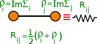
Figure 3: Square resistor network in which each resistor couples two neighboring sites.

The various resistors are connected through the geometry of the network. At the ends of the network external resistors are placed that are connected to external voltages $\phi_{i}$. These external resistor values are given by the resistivities at the edge sites. The external voltages are fixed as $\phi_{0}$ at the left edge and $\phi$ at the right edge. The network of resistors has the form shown in Fig. 4 for the particular case of a $3x3$ network. The internal voltages and currents, which pass through each resistor are unknown and need to be determined using electrical circuit theory.

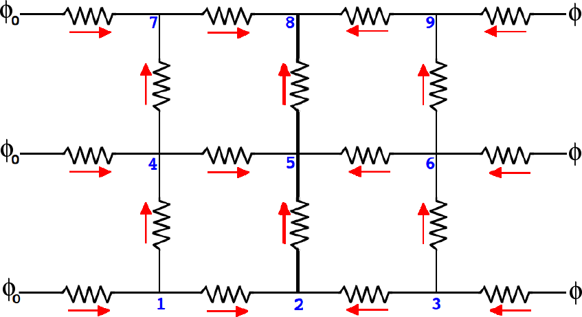
Figure 4: Resistors associated to a 3 x 3 square network.

In general, for a network with $LxL$ sites, the total number of nodes is $2L+L{{}^{2}}$, with $L^{2}$ internal nodes and $2L$ external nodes. The total number of resistors is $2L{{}^{2}}$. We need to find the $2L^{2}$ currents $I_{ij}$ that cross the resistors and the $L^{2}$ voltages at each internal node. In all, therefore, there are $3L{{}^{2}}$ unknowns. The current at the inner nodes is conserved (Kirchhoff’s law) providing $L^{2}$ equations

$$\sum_{j}I_{ij}=0.$$ (26)

For each resistor, we apply Ohm’s law

$$I_{ij}=\frac{V_{i}-V_{j}}{R_{ij}},$$ (27)

which gives us $2L^{2}$ equations. We therefore have a total of $3L^{2}$ equations for $3L^{2}$ unknowns. We found the solutions numerically.

VI Results and Discussion

To describe the Mott transition in two dimensions we use the Hubbard Hamiltonian in the two dimensional square lattice given in Eq. (1). Several studies of the clean case have established the first-order nature of the transition at finite temperatures below $T_{c}$, with the corresponding coexistence region and associated hysteresis (Vucicević et al., 2013; Terletska et al., 2011; Dobrosavljevic et al., 2012; Miranda et al., 2008). For a finite-size system, we expect the hysteresis to survive. Therefore, we have to allow for the convergence of both stable and meta-stable solutions to the statDMFT equations. We thus start from initial $U$ values which are safely outside the coexistence region, either in metallic or in the insulating phase. For a given interaction value $U_{0}$ the values of $G_{i}(i\omega_{n})$ are found once convergence has been achieved. The results of $G_{i}(i\omega_{n})$ for $U_{0}$ are used as an initial guess for $G_{i}(i\omega_{n})$ at $U_{1}=U_{0}+\Delta U$ (going from the metal to the insulator) or $U_{1}=U_{0}-\Delta U$ (going from the insulator to the metal). The new results for $G_{i}(i\omega_{n})$ are used to generate the $G_{i}(i\omega_{n})$ corresponding to the next value $U_{2}$ and thus consecutively, doing a scan of $U$ values from the metal to the insulator or from the insulator to the metal.

As $U$ is scanned an abrupt jump is observed in $ImG(\omega_{1})$. We define $U_{c1}$ to be this critical jump value when going from insulator to metal and $U_{c2}$ to represent the value when going from metal to insulator. These are the so-called spinodals. The difference of paths traveled going from metal to insulator and from insulator to metal defines hysteresis curves, such as shown in Fig 5, for the clean case. The region that is contained between $U_{c1}$ and $U_{c2}$ is the coexistence region, in which one of the solutions is only meta-stable. In the coexistence region, for a value of $U$, it is possible to find the two behaviors, metallic and insulating.

The disordered case is shown in the Fig. 6. Note that, since $G_{i}(i\omega_{n})$ now fluctuates spatially we have shown all the $L^{2}$ curves for $-\mathrm{Im}G_{i}\left(i\omega_{1}\right)$. Although there are many curves, a clear hysteretic behavior is apparent, especially at the lowest temperatures. Besides, adding disorder causes a shift in the hysteresis curves to higher interaction values and the coexistence region shrinks in size.

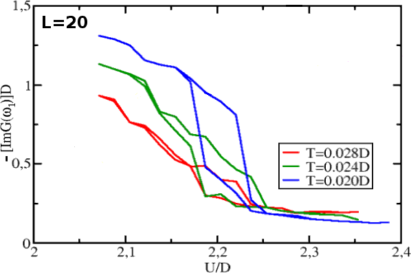
Figure 5: Hysteresis curves for different temperature values, below the critical point of clean Mott transition. As the temperature increases, the hysteresis loops become smaller.

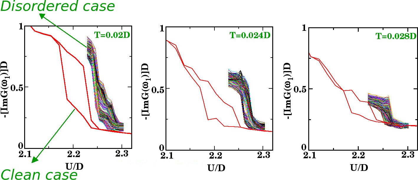
Figure 6: Hysteresis curves for different values of temperature. Notice how the disorder shifts the hysteresis curve to higher values of interaction energy, while the coexistence region shrinks.

Let us now focus on the vicinity of the Mott transition. For each value of $U$ in a scan of values where $\Delta U=0.008D$, a map is obtained representing the spatial behavior of the imaginary part of the Green’s function at the first Matsubara frequency. Fig 7 shows these results for $T=0.024D$ going from the metal to the insulator (Results for other values of temperature, can be found in the Supplementary Material (SMa, )). The color scale is organized so that the largest value of $-\mathrm{Im}G(\omega_{1})$ corresponds to red and the smallest values to blue. As the value of the local interaction changes, the spatial configuration in the lattice changes. The system, which initially was a metal with significant spatial homogeneity, begins to show “bubbles” corresponding to insulating regions. Finally, these coalesce to form a rather homogeneous insulator. Similarly, starting with high local electron-electron interaction it is observed that, as the value of the local interactions decrease, metallic "bubbles" appear until the lattice becomes metallic, as shown in Fig 8. Comparing the same intermediate values of $U$ in the two figures, we can easily distinguish the two coexisting solutions.

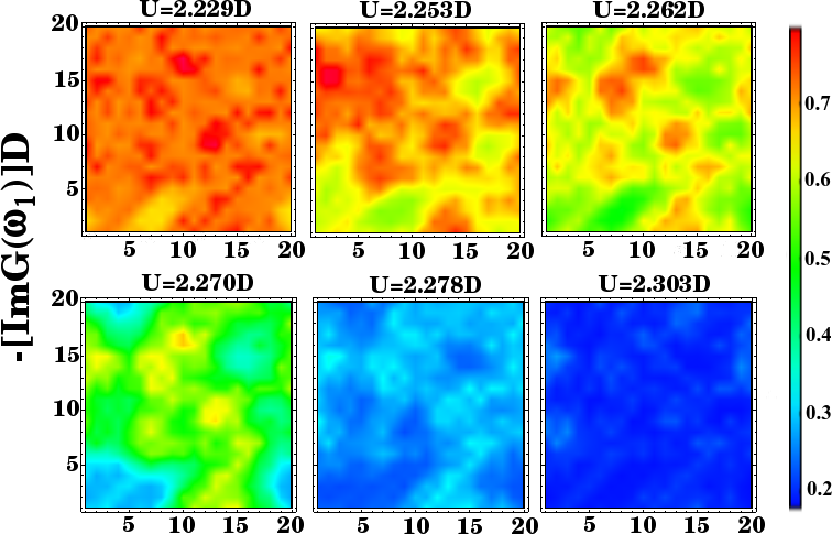
Figure 7: Imaginary part of the Green’s function at the first Matsubara frequency for each site of the square lattice with $T=0.024D$ in the neighborhood of the Mott transition when going from the metal to the insulator. See video mi.avi at Supplementary Material (SMa, ).

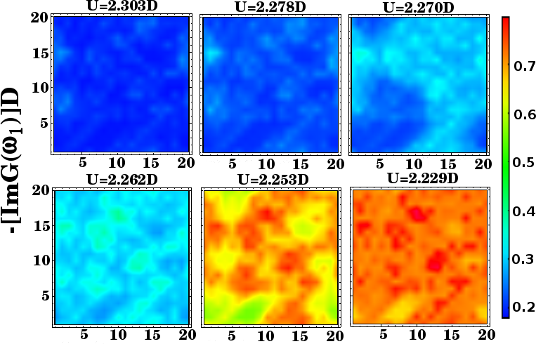
Figure 8: Imaginary part of the Green’s function at the first Matsubara frequency for each site of the lattice for $T=0.024D$ and a scan of values of $U$ in the neighborhood of the Mott transition going from the insulator to the metal. See video im.avi at Supplementary Material (SMa, ).

VI.1 Critical behavior of the Mott transition

We now focus on the correlations between the fluctuations of the bare disorder and the local order parameter of the Mott transition. Fig. 9 shows the spatial patterns of the local order parameter $\mathrm{-Im}G_{i}(i\omega_{1})$ for four different disorder realizations at $W=0.52D$, $U=2.27D$ and $T=0.024D$. The range of variations for each disorder realization is between $0.20<[-\mathrm{Im}G(\omega_{1})]D<0.57$. The red color represents the regions with greater metallic behavior and blue regions represent the insulator. For convenience, let us define an essentially metallic region as one in which the condition $[-ImG(\omega_{1})]D>0.45$ is satisfied. Analogously, essentially insulating regions are defined as those in which $[-ImG(\omega_{1})]D<0.27$. In each of these regions we calculate the relative local fluctuation of the disorder $\Delta\epsilon/\Delta\epsilon_{distr}$, where we take $\bar{\epsilon}=0$, $\Delta\epsilon=\sqrt{\frac{\overset{N}{\underset{i=1}{\sum}}\epsilon_{i}^{2}}{N-1}}$ and the standard deviation of the bare distribution is $\Delta\epsilon_{distr}=\sqrt{\frac{W^{2}}{12}}=0.15D$.

Figure 9: For four different realizations of disorder, we show $\mathrm{Im}G_{i}(\omega_{1})$ via a color scale. The red color represents the lattice sites that have metallic behavior. Insulating behavior corresponds to blue regions. We used $W=0.52D$, $U=2.27D$ and $T=0.024D$.

Table 1 shows the results for the $\Delta\epsilon/\Delta\epsilon_{distr}$ for each one of the regions. In the insulating regions, where $0.20\leq[-ImG(\omega_{1})]D\leq 0.27$, the values of $\Delta\epsilon/\Delta\epsilon_{distr}$ are always smaller than 1. The values $\Delta\epsilon/\Delta\epsilon_{distr}$ in the metallic regions, where $0.45<[-ImG(\omega_{1})]D<0.57$, on the other hand are all larger than 1. There is a strong correlation between small (large) values of $\Delta\epsilon$ and insulating behavior (metallic). In the regions with intermediate behavior $\Delta\epsilon\simeq\Delta\epsilon_{distr}$. These results are in qualitative agreement with the analysis of reference Liu et al., 2016 of the insulating and metallic puddles of VO₂, which showed that the observed scaling behavior is best described by the critical random field Ising model. Unfortunately, we cannot access very large lattice sizes in order to be able to do a full scaling analysis of the puddle sizes.

	Insulator	Intermediate regime	Metal
Intervals	$A$	$B$	$C$
Number 1$\Delta\epsilon/\Delta\epsilon_{distr}$	$0.79$	$0.88$	$1.28$
Number of sites	$7$	$273$	$120$
Number 2 $\Delta\epsilon/\Delta\epsilon_{distr}$	$0.75$	$0.93$	$1.36$
Number of sites	$75$	$262$	$63$
Number 3 $\Delta\epsilon/\Delta\epsilon_{distr}$	$0.81$	$0.90$	$1.33$
Number of sites	$74$	$264$	$62$
Number 4 $\Delta\epsilon/\Delta\epsilon_{distr}$	$0.73$	$0.93$	$1.30$
Number of sites	$76$	$264$	$60$

Table 1: Fluctuations of $\Delta\epsilon$ for the insulating, metallic and intermediate regions, corresponding to the different disorder realizations of Fig. 9. Here $A=0.20\leq[-\mathrm{Im}G(\omega_{1})]D\leq 0.27$, $B=0.27<[-\mathrm{Im}G(\omega_{1})]D<0.45$ and $C=0.45\leq[-\mathrm{Im}G(\omega_{1})]D\leq 0.57$

VI.2 Finite-size effects

The Mott transition is smeared in the thermodynamic limit in $d=2$, since there is a proliferation of metallic and insulating regions when $L\rightarrow\infty$. Let us now study how our results change as we increase $L$.

Fig 10 shows a set of hysteresis curves for different lattices sizes, at $T=0.024D$ and $W=0.52D$. It is observed that the $U/D$ values at which the Mott transition occurs are the same independently of the lattice size, while the values of $[-\mathrm{Im}G(\omega_{1})]D$ remain between $0.2$ and $0.8$. Note that in the case where we have a square lattice of $10\times 10$ sites, the size of the coexistence region is larger than for larger lattice sizes. Furthermore, the first-order Mott transition becomes a “rounded” transition as $L\rightarrow\infty$, in accordance with the generalized Imry and Ma theorem for the disordered Hubbard model. Unfortunately, it is computationally very difficult to obtain results for $L>20$.

Figure 10: Hysteresis loops for different lattice sizes, below the critical point of Mott transition. As the temperature increases, the hysteresis loops become smaller.

Now we focus on a particular Coulomb interaction value $U=2.27D$ and we analyze the spatial pattern of $\mathrm{Im}G_{i}\left(i\omega_{1}\right)$, as shown in Fig.11 for $T=0.024D$, in the upper branch of the hysteresis loop (for other temperature values see the Supplementary Material (SMa, )). Notice how as the size of the lattice increases, metallic regions persist at the same positions, but also note the appearance of insulating bubbles. In the thermodynamic limit we have the proliferation of metallic and insulating regions and the complete smearing of the transition. Again, we note that both the inhomogeneous state with coexisting bubbles and the accordance with the Imry-Ma theorem are in agreement with the picture of the transition in VO₂ as being in the same universality class as the random field Ising model (Liu et al., 2016).

Figure 11: Finite-size effects: Spatial pattern of $\mathrm{Im}G_{i}\left(i\omega_{1}\right)$ for different sizes of the square lattice. Metallic and insulating bubbles proliferate as the lattice increases at $U=2.27D$ in the upper branch of the hysteresis loop.

At this point, let us make some remarks regarding the difference between the clean and disordered cases. In the clean Hubbard model close to the Mott transition, thermal fluctuations also generate metallic and insulating bubbles (Papanikolaou et al., 2008; Helmes, 2008; Liu, 2012). Their frequency and size are determined by a Boltzmann factor. In the disordered case, however, the bubbles are nucleated by the interplay of both temperature and local fluctuations of the disorder potential, with the latter playing a dominant role. That can be roughly gleaned from the persistence of the bubble landscape as the temperature is varied with a fixed disorder realization (see Fig. 1 of the Supplemental Material (SMa, )). Furthermore, the correlation between the size of the site-energy fluctuations and the nature of the bubbles (Table I) corroborates this conclusion. Finally, in the 2D case we focus on here, the first-order transition is destroyed by disorder. We conclude that the nature and features of the bubbles are very different in the clean and the disordered cases.

VI.3 Transport in the lattice

To study the transport properties we analyzed the quantity $l_{in}=\frac{D}{\mathrm{Im}\Sigma}$ as described in Eq. (24) through statDMFT. The lowest frequency that can be used in this case is the first Matsubara frequency. Thus, we use $\Sigma_{i}(i\omega_{1})$ as an estimate of $\Sigma_{i}(\omega\rightarrow 0)$. Fig. 12, depicts the value $\frac{Im\Sigma(i\omega_{1})}{D}$, for $T=0.024D$ and $W=0.52D$, for each site of the lattice and value of interaction $U$, in the vicinity of the Mott transition. Notice that $0.98\leq\frac{Im\Sigma(i\omega_{1})}{D}\leq 5.09$, or $0.2\lesssim\frac{D}{Im\Sigma(i\omega_{1})}\lesssim 1$. According to Eq. (24) from Section V, this corresponds to $l_{in}\lesssim a$. Therefore, we can describe transport classically at all scales.

Figure 12: Imaginary part of self-energy for the first Matsubara frequency for $T=0.024D$.

Using Eq (25) to find the values of the equivalent resistors in the square lattice and Eq. (27) to calculate $I_{ij}$ between the nodes, it is possible to find the mean value of the current in each node $I(i)=\frac{\Sigma_{j}|I_{ij}|}{N_{s}}$ , where $N_{s}$ is the number of resistors that are connected to a given node. In Fig. 13 we present the results of the spatial mapping of the current at $T=0.024D$ and $W=0.52D$, in the vicinity of the Mott transition (The Supplementary Material (SMa, ) shows solutions for other temperatures). The red color represents regions in which the current presents higher values. Low values of the current are represented by the blue color and are associated with insulating behavior. We note that the current is not uniform in the system and has spatial fluctuations. However, its variations are mild and the values decrease with increasing $U$.

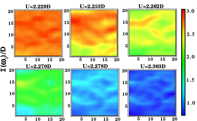
Figure 13: Spatial mapping of the current in the vicinity of the Mott transition for $T=0.024D$.

After calculating the value of the average current for each of lattice site, we can find the average value over the complete network for each interaction value $U$ in the vicinity of Mott transition. The variation of the mean current is large for the case of $T=0.02D$ (see Supplementary Material (SMa, ), for more details). As the temperature increases the current in the transition region still presents a noticeable change, but it is much milder than in the case of $T=0.02D$. Since the external potentials used in the calculations are fixed, the average current is a measure of the conductance $G=\frac{I}{(\Phi-\Phi_{0})}$ . We note that, although the conductance has a strong dependence on temperature in the metallic regime, it is almost independent of $T$ in the insulating regime. This is a consequence of the fact that $\mathrm{Im}G_{i}\left(i\omega_{1}\right)$ cannot capture the exponential dependence with the temperature that comes from the presence of the Mott gap.

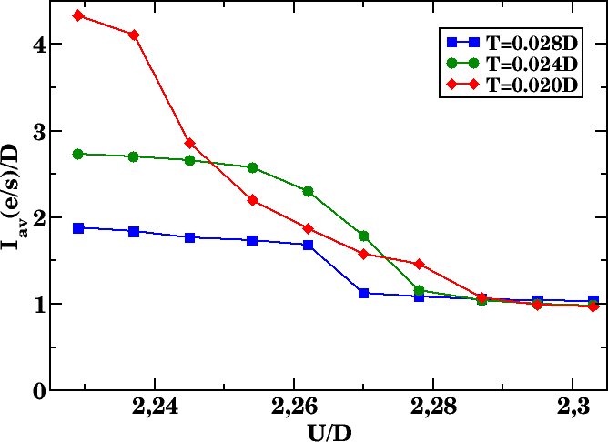
Figure 14: Average current as a function of Coulomb potential in the transition region of Mott for different temperature values.

VII Conclusions

Using DMFT, in the clean case, and statDMFT, in the disordered case, it was possible to analyze the Mott transition in Hubbard model in a square lattice. In finite-sized lattices, disorder does not destroy the first-order character of the transition with the accompanying hysteresis loop and coexisting metallic and insulating solutions. Since the local Green’s function now has spatial fluctuations, however, there is a different hysteresis loop on each site. The bundle of loops shows an overall shift towards higher values of interactions when compared with the clean case. The spatial pattern found shows clearly the coexistence in each solution of metallic as well as insulating “bubbles”. As the system size increases, these different “bubbles” proliferate and point to a complete smearing of the first-order transition in the thermodynamic limit, in complete agreement with the Imry-Ma theorem. The statistics of local bare disorder fluctuations correlate also reasonably well with metallic or insulating nature of the inhomogeneities, which strengthens the link between the metal-insulator transition in the disordered Hubbard model and the one of the random field Ising model. Such a link had been previously emphasized in a scaling analysis of the experimental results on the metal-insulator transition in VO₂.(Liu et al., 2016) Finally, we performed the first calculation of transport properties within the statDMFT. This was possible only because the analyzed system is a highly incoherent one, where $k_{F}l_{in}\sim a$, and the calculation could be done through a mapping of the system onto a random network of classical resistors. After this mapping, the global resistance could be calculated and the temperature dependence in the metal is in agreement with expectations. The same description fails in the insulating case, however, where we expect to see an activated temperature dependence.

Our work offers a powerful theoretical perspective on spatial inhomogeneities of disordered strongly correlated systems. In this sense, it is a welcome contribution to the description of the detailed experimental results coming from recent nano-imaging techniques. Besides the interplay of disorder and Mott physics explored in this work, we envisage important directions for future work. In the particularly well-studied example of VO₂(Park et al., 2013; Liu et al., 2013) as well as in other compounds(Pustogow et al., 2018) the coupling between electronic and structural degrees of freedom is probably important and could be incorporated. The inhomogeneous nanoscale patterns of systems with competing orders, such as high-T_c cuprates(Campi et al., 2015) and iron-based superconductors(Allan et al., 2013) would also benefit from the kinds of insights gained from our approach. As these experimental techniques mature, we expect more examples will be found where our approach may prove useful.

VIII acknowledgments

We acknowledge support by CNPq (Brazil) through Grants No. 307041/2017-4 and No. 590093/2011-8, Capes (Brazil) through grant 0899/2018 (E.M.), NSF (USA) through Grant DMR-1822258 (V.D. and T-H.L), Texas Center for Superconductivity at the University of Houston, University of Houston Health Research Institute, the Center for Bioenergetics at Houston Methodist Research Institute, and Leonardo Machado for the helpful feedback (M.Y.S.V and J.H.M).

References

- Rosenbaum et al. (1983) T. F. Rosenbaum, R. F. Milligan, M. A. Paalanen, G. A. Thomas, R. N. Bhatt, and W. Lin, Phys. Rev. B 27, 7509 (1983).
- M. A. Paalanen (1991) R. M. A. Paalanen, Physica B 169, 223 (1991).
- Anissimova et al. (2007) S. Anissimova, S. V. Kravchenko, A. Punnoose, A. Finkel’stein, and T. Klapwijk, Nature Phys 3, 707 (2007).
- Hanein et al. (1998) Y. Hanein, U. Meirav, D. Shahar, C. Li, D. Tsui, and H. Shtrikman, Phys. Rev. Lett. 80, 1288 (1998).
- Lilly et al. (2003) M. P. Lilly, J. L. Reno, J. A. Simmons, I. B. Spielman, J. P. Eisenstein, L. N. Pfeiffer, K. W. West, E. H. Hwang, and S. D. Sarma, Phys. Rev. Lett. 90, 056806 (2003).
- Lederer et al. (1972) P. Lederer, H. Launois, J. P. Pouget, and A. C. G. Villeneuve, Journal of Physics and Chemical of Solid 33, 1969 (1972).
- J. Mazzaferro (1980) B. J. Mazzaferro, H. Ceva, Phys. Rev. B. 22, 353 (1980).
- Limelette et al. (2003) P. Limelette, P. Wzietek, S. Florens, A. Georges, T. A. Costi, C. Pasquier, D. Jerome, C. Meziere, and P. Batail, Phys. Rev. Lett. 91, 016401 (2003).
- Liu et al. (2017) M. Liu, A. J. Sternbach, and D. N. Basov, Rep. Prog. Phys. 80, 014501 (2017).
- Qazilbash et al. (2007) M. Qazilbash, M. Brehm, C. Byung-Gyu, P.-C. Ho, G. O. Andreev, K. Bong-Jun, S. J. Yun, A. V. Balatsky, M. B. Maple, F. Keilmann, et al., Science 318, 1750 (2007).
- Qazilbash et al. (2009) M. M. Qazilbash, M. Brehm, G. O. Andreev, A. Frenzel, P.-C. Ho, B.-G. Chae, B.-J. Kim, S. J. Yun, H.-T. Kim, A. V. Balatsky, et al., Phys. Rev. B 79, 075107 (2009).
- O’Callahan et al. (2015) B. T. O’Callahan, A. C. Jones, J. H. Park, D. H. Cobden, J. M. Atkin, and M. B. Raschke, Nat. Commun. 6, 6849 (2015).
- Liu et al. (2013) M. K. Liu, M. Wagner, E. Abreu, S. Kittiwatanakul, Z. F. A. McLeod, M. Goldflam, S. Dai, M. M. Fogler, J. Lu, S. A. Wolf, et al., Phys. Rev. Lett. 111, 096602 (2013).
- P.W.Anderson (1958) P.W.Anderson, Phys. Rev. 109, 1492 (1958).
- Abrahams et al. (1979) E. Abrahams, P. W. Anderson, D. C. Licciardello, and T. V. Ramakrishnan, Phys. Rev. Lett. 42, 673 (1979).
- Mott (1990) N. F. Mott, Metal-Insulator transition (Taylor & Francis, London, 1990).
- Hubbard (1963) J. Hubbard, Proc. R. Soc. (London) A 276, 238 (1963).
- Hubbard (1964a) J. Hubbard, Proc. Roy. Soc. (London) A 277, 237 (1964a).
- Hubbard (1964b) J. Hubbard, Proc. Roy. Soc. (London) A 281, 401 (1964b).
- Lee and Ramakrishnan (1985) P. A. Lee and T. V. Ramakrishnan, Rev. Mod. Phys. 57, 287 (1985).
- Altshuler and Aronov (1979) B. L. Altshuler and A. G. Aronov, Solid State Commun. 30, 115 (1979).
- Castellani et al. (1984) C. Castellani, C. D. Castro, P. A. Lee, and M. Ma, Phys. Rev. B 30, 527 (1984).
- Castellani et al. (1987) C. Castellani, B. G. Kotliar, and P. A. Lee., Phys. Rev. Lett. 56, 1179 (1987).
- Brinkman and Rice (1970) W. F. Brinkman and T. M. Rice, Phys. Rev. B 2, 4302 (1970).
- Gutzwiller (1963) M. C. Gutzwiller, Phys. Rev. Lett. 10, 159 (1963).
- Gutzwiller (1964) M. C. Gutzwiller, Phys. Rev. 134, A923 (1964).
- Gutzwiller (1965) M. C. Gutzwiller, Phys. Rev. 137, A1726 (1965).
- Metzner and Vollhardt (1989) W. Metzner and D. Vollhardt, Phys. Rev. Lett. 62, 324 (1989).
- Georges et al. (1996) A. Georges, G. Kotliar, W. Krauth, and M. Rozenberg, Rev. Mod. Phys. 68, 13 (1996).
- Kotlyar and Das Sarma (2001) R. Kotlyar and S. Das Sarma, Phys. Rev. Lett. 86, 2388 (2001).
- Ulmke and Scalettar (1997) M. Ulmke and R. T. Scalettar, Phys. Rev. B 55, 4149 (1997).
- Denteneer et al. (1999) P. J. H. Denteneer, R. T. Scalettar, and N. Trivedi, Phys. Rev. Lett. 83, 4610 (1999).
- Paris et al. (2007) N. Paris, A. Baldwin, and R. T. Scalettar, Phys. Rev. B 75, 165113 (2007).
- Srinivasan et al. (2003) B. Srinivasan, G. Benenti, and D. L. Shepelyansky, Phys. Rev. B 67, 205112 (2003).
- Chang and Scalettar (2012) C.-C. Chang and R. T. Scalettar, Phys. Rev. Lett. 109, 026404 (2012).
- Heidarian and Trivedi (2004) D. Heidarian and N. Trivedi, Phys. Rev. Lett. 93, 126401 (2004).
- Shinaoka and Imada (2009) H. Shinaoka and M. Imada, J. Phys. Soc. Jpn. 78, 094708 (2009).
- Shinaoka and Imada (2010) H. Shinaoka and M. Imada, J. Phys. Soc. Jpn. 79, 094711 (2010).
- Pezzoli and Becca (2010) M. E. Pezzoli and F. Becca, Phys. Rev. B 81, 075106 (2010).
- Ulmke et al. (1995) M. Ulmke, V. Janiš, and D. Vollhardt, Phys. Rev. B 51, 10411 (1995).
- Tanasković et al. (2003) D. Tanasković, V. Dobrosavljević, E. Abrahams, and G. Kotliar, Phys. Rev. Lett. 91, 066603 (2003).
- Aguiar et al. (2005) M. C. O. Aguiar, V. Dobrosavljević, E. Abrahams, and G. Kotliar, Phys. Rev. B 71, 205115 (2005).
- Andrade et al. (2009) E. C. Andrade, E. Miranda, and V. Dobrosavljević, Phys. Rev. Lett. 102, 206403 (2009).
- Dobrosavljevic et al. (2003) V. Dobrosavljevic, A. A. Pastor, and B. K. Nikolić, EPL 62, 72 (2003).
- Byczuk et al. (2005) K. Byczuk, W. Hofstetter, and D. Vollhardt, Phys. Rev. Lett. 94, 056404 (2005).
- Byczuk et al. (2009) K. Byczuk, W. Hofstetter, and D. Vollhardt, Phys. Rev. Lett. 102, 146403 (2009).
- Dobrosavljevic (2010) V. Dobrosavljevic, International Journal of Modern Physics B 24, 1680 (2010).
- Sen et al. (2016) S. Sen, H. Terletska, J. Moreno, N. S. Vidhyadhiraja, and M. Jarrell, Phys. Rev. B 94, 235104 (2016).
- Sen et al. (2018) S. Sen, N. S. Vidhyadhiraja, and M. Jarrell, Phys. Rev. B 98, 075112 (2018).
- Benenti et al. (1999) G. Benenti, X. Waintal, and J.-L. Pichard, Phys. Rev. Lett. 83, 1826 (1999).
- Punnoose and Finkel’stein (2005) A. Punnoose and A. M. Finkel’stein, Science 310, 289 (2005).
- Dobrosavljevic and Kotliar (1997) V. Dobrosavljevic and G. Kotliar, Phys. Rev. Lett 78, 3943 (1997).
- Hirsch and Fye. (1986) J. E. Hirsch and R. M. Fye., Phys. Rev. Lett 56, 2521 (1986).
- Potthoff and Nolting (1999) M. Potthoff and W. Nolting, Phys. Rev. B 59, 2549 (1999).
- Miller and Freericks (2001) P. Miller and J. K. Freericks, J. Phys.: Condens. Matter 13, 3187 (2001).
- Freericks (2004) J. K. Freericks, Phys. Rev. B 70, 195342 (2004).
- Okamoto and Millis (2005) S. Okamoto and A. J. Millis, Phys. Rev. B 72, 235108 (2005).
- Chen and Freericks (2007) L. Chen and J. K. Freericks, Phys. Rev. B 75, 125114 (2007).
- Florens (2007) S. Florens, Phys. Rev. Lett. 99, 046402 (2007).
- Snoek et al. (2008) M. Snoek, I. Titvinidze, C. Tőke, K. Byczuk, and W. Hofstetter, New Journal of Physics 10, 093008 (2008).
- Helmes et al. (2008a) R. W. Helmes, T. A. Costi, and A. Rosch, Phys. Rev. Lett. 100, 056403 (2008a).
- Helmes et al. (2008b) R. W. Helmes, T. A. Costi, and A. Rosch, Phys. Rev. Lett. 101, 066802 (2008b).
- Gorelik et al. (2010) E. V. Gorelik, I. Titvinidze, W. Hofstetter, M. Snoek, and N. Blümer, Phys. Rev. Lett. 105, 065301 (2010).
- Byczuk et al. (2019) K. Byczuk, B. Chatterjee, and D. Vollhardt, Eur. Phys. J. B 92, 93 (2019).
- Kotliar et al. (2000) G. Kotliar, E. Lange, and M. J. Rozenberg, Phys. Rev. Lett 84, 5180 (2000).
- See and e. g (1997) See and e. g, World Scientific p. 277 (1997).
- Liu et al. (2016) S. Liu, B. Phillabaum, E. W. Carlson, K. A. Dahmen, N. S. Vidhyadhiraja, M. M. Qazilbash, and D. N. Basov, Phys. Rev. Lett 116, 036401 (2016).
- Imry and Ma (1975) Y. Imry and S. K. Ma, Phys. Rev. Lett 35, 1399 (1975).
- Trivedi and Randeria (1995) N. Trivedi and M. Randeria, Phys. Rev. Lett. 75, 312 (1995).
- Landauer (1970) R. Landauer, Philos. Mag 21, 863 (1970).
- Meir and Wingreen (1992) Y. Meir and N. S. Wingreen, Phys. Rev. Lett. 68, 2512 (1992).
- Fetter and Walecka (1970) A. Fetter and J. Walecka, Philos. Mag 21, 863 (1970).
- Vucicević et al. (2013) J. Vucicević, H. Terletska, D. Tanasković, and V. Dobrosavljevic, Phys. Rev. B 88, 075143 (2013).
- Terletska et al. (2011) H. Terletska, J.Vucicevic, D.Tanaskovic, and V.Dobrosavljevic, Phys. Rev. Lett 84, 125120 (2011).
- Dobrosavljevic et al. (2012) N. T. V. Dobrosavljevic, J. James, and M. Valles, Oxford University p. USA (2012).
- Miranda et al. (2008) E. Miranda, D. Garcia, and M. R. K. Hallberg, Physica B: Condensed Matter 403, 1465 (2008).
- (77) See Supplemental Material at http://link.aps.org/supplemental/ 10.1103/PhysRevB.101.235112, for details about StatDMFT at different temperatures and other values of disorder.
- Papanikolaou et al. (2008) S. Papanikolaou, R. M. Fernandes, E. Fradkin, P. W. Phillips, J. Schmalian, and R. Sknepnek, Phys. Rev. Lett. 100, 026408 (2008).
- Helmes (2008) R. Helmes, Ph.D. thesis, University of Cologne (2008), URL https://kups.ub.uni-koeln.de/2260/.
- Liu (2012) Q. Liu, Ph.D. thesis, University of Bonn (2012), URL http://hss.ulb.uni-bonn.de/2012/2929/2929.htm.
- Park et al. (2013) J. H. Park, J. M. Coy, T. S. Kasirga, C. Huang, and S. Z. Fei, Nature 500, 431 (2013).
- Pustogow et al. (2018) A. Pustogow, A. S. McLeod, Y. Saito, D. N. Basov, and M. Dressel, Sci. Adv. 4, eaau9123 (2018).
- Campi et al. (2015) G. Campi, A. Bianconi, N. Poccia, G. Bianconi, L. Barba, G. Arrighetti, D. Innocenti, J. Karpinski, N. D. Zhigadlo, S. M. Kazakov, et al., Nature 525, 359 (2015).
- Allan et al. (2013) M. P. Allan, T.-M. Chuang, F. Massee, Y. Xie, N. Ni, S. L. Budko, G. S. Boebinger, Q. Wang, D. S. Dessau, P. C. Canfield, et al., Nature Phys 9, 220 (2013).