Tuning the random walk of active colloids

Abstract

Active particles such as swimming bacteria or self-propelled colloids are known to spontaneously organize into fascinating large-scale dynamic structures. The emergence of these collective states from the motility pattern of the individual particles, typically a random walk, is yet to be probed in a well-defined synthetic system. Here, we report the experimental realization of intermittent colloidal motion that reproduces the run-and-tumble and Lévy trajectories common to many swimming and swarming bacteria. Our strategy enables to tailor the sequence of repeated “runs” (nearly constant-speed straight-line translation) and “tumbles” (seemingly erratic turn) to emulate any random walk. This new paradigm for active locomotion at the microscale opens new opportunities for experimental explorations of the collective dynamics emerging in active suspensions. We find that population of these random walkers exhibit behaviors reminiscent of bacterial suspensions such as dynamic clusters and mesoscale turbulent-like flows.

Swimming bacteria navigate their environment by executing random walks Elgeti et al. (2015); Lauga (2016). In a general run-and-turn type, persistent swimming is interrupted by random changes in the direction of motion. Examples include the widely studied run-and-tumble E. coli Berg and Brown (1972), run-and-active-stop R. sphaeroides Pilizota et al. (2009), run-and-reverse P. putida Theves et al. (2013), and run-reverse-flick V. alginolyticus Xie et al. (2011). These motility strategies have inspired great interest in the engineering of artificial self-propelled particles that mimic the elaborate locomotion patterns of their biological counterparts Ebbens and Gregory (2018); Han et al. (2018); Palagi and Fischer (2018); Huang et al. (2019). Most available experimental designs of artificial colloidal microswimmers perform active Brownian motion Paxton et al. (2004); Fournier-Bidoz et al. (2005); Howse et al. (2007); Jiang et al. (2010); Buttinoni et al. (2012); Baraban et al. (2013); Samin and van Roij (2015); Gomez-Solano et al. (2016); Narinder et al. (2018), where the reorientation in the directed motion is driven by the rotational diffusion of the swimmer. This results in slow and continuous directional changes, in contrast to the sudden turning events characteristic of the run-and-tumble bacteria. Efforts to emulate the kinetics of the bacterial run-and-tumble motions Ebbens et al. (2010, 2012); Mano et al. (2017) have been unable to achieve truly random reorientation events with controllable turn time. Only recently, reorientation disentangled from rotational diffusion has been accomplished by triggering elastic recoil in a non-Newtonian fluid suspending the motile colloid Celia Lozano and Bechinger (2018). However, this approach does not allow to change the duration of the turn step as it is set by the elastic relaxation time of the fluid.

Here we report the experimental realization of a motile colloid, inspired by the Quincke roller Bricard et al. (2013, 2015); Pradillo et al. (2019), that performs finely–tunable, diverse random walks such as run-and-tumble or Lévy walks (Fig. 1b, Fig. 2b,g). A population of the Quincke random walkers display collective dynamics reminiscent of bacterial suspensions such as self-organization into large–scale aggregates and turbulent–like flows. They form swarms, rotating clusters, polar clusters cruising over the whole domain without significant exchange of particles and dynamic disordered clusters that continuously deform and break by exchanging particles.

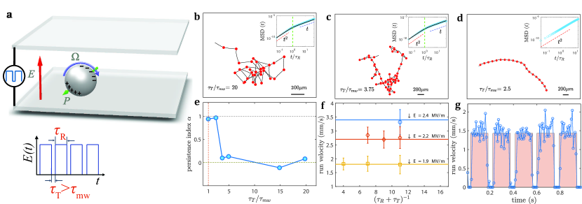
Figure 1: (a) Quincke rotation: In a uniform dc electric field, free charges brought by conduction accumulate at the particle surface. A spontaneous symmetry breaking of the charge distribution gives rise to a net torque and the sphere spins at a rate ${\bm{\Omega}}$ about a randomly chosen axis in the plane perpendicular to the applied field direction. Experimental set-up: An insulating colloidal sphere is resting on the bottom electrode of a parallel-plate chamber filled with weakly-conducting oil. A uniform electric field $E$ with magnitude above the threshold for Quincke rotation is applied to cause the sphere to roll. If a square-wave electric field is applied with period between the pulses longer than the time needed for the sphere to depolarize (Maxwell-Wagner time), the sphere executes a random walk. (b-d) Quincke walker trajectories at different $\tau_{T}/\tau_{\mathrm{mw}}$ ratios, with $\tau_{R}=0.15$ s. Particle stops are marked with red circles. Insets: log-log plot of time-averaged experimental (symbol) and theoretical (solid line) mean-square displacement (crossover marked by the vertical dashed line at $t=\tau_{R}$). (e) persistence index $\alpha$ for different $\tau_{T}/\tau_{\mathrm{mw}}$ ratios. (f) Run velocity depends solely on the amplitude of the applied electric field. Symbols: measured velocity at different amplitude and frequencies $1/(\tau_{R}+\tau_{T})$ of the applied pulsed signal; Solid lines: velocity measured in dc fields. (g) particle velocity for 1 second duration of the pulsed signal, $\tau_{T}/\tau_{\mathrm{mw}}=20$, $\tau_{R}=0.15$ s. E=1.66 MV/m.

The colloid “run” is powered by Quincke rotation, i.e., the spontaneous spinning of a particle polarized in a uniform DC electric field Quincke (1896) (see Fig. 1a and Appendix for a detailed description of the phenomenon). If the sphere is on a surface, it rolls steadily following a straight trajectory. The Quincke rollers have stirred a lot of interest since they were discovered to undergo collective directed motion Bricard et al. (2013, 2015); Morin et al. (2017a); Geyer et al. (2018). Our strategy to introduce a “tumble” in the colloid trajectory exploits a unique feature of the Quincke instability: the degeneracy of the rotation axis in the plane perpendicular to the applied electric field (and parallel to the rolling surface). A sequence of on-off-on electric field causes the sphere to roll-stop-turn; the turn is due to the Quincke instability picking a new axis of rotation. One caveat, though, is that the charging and discharging of the particle occurs by conduction and require finite time. The induced dipole ${\bf{P}}$ evolves as Lemaire and Lobry (2002)

$$\frac{\partial{\bf{P}}}{\partial t}={\bm{\Omega}}\times{\bf{P}}-\tau_{\mathrm{mw}}^{-1}\left({\bf{P}}-\chi_{e}{\bf E}\right)\,.$$ (1)

where ${\bm{\Omega}}$ is the rotation rate and $\chi_{e}$ is the electric susceptibility of the particle. The characteristic time scale for polarization relaxation is the Maxwell-Wagner time $\tau_{\mathrm{mw}}=({\varepsilon}_{\mathrm{p}}+2{\varepsilon}_{\mathrm{s}})/(\sigma_{\mathrm{p}}+2\sigma_{\mathrm{s}})$, which depends solely on the fluid and particle conductivities and permittivities, $\sigma$ and ${\varepsilon}$. Random reorientation after each run is only ensured if the sphere is completely discharged before the field is turned on. Incomplete depolarization acts as a memory and correlates subsequent runs. Thus the relaxation nature of the polarization adds another functionality to the Quincke walks: variable degree of run correlation. Furthermore, since the Maxwell-Wagner “memory” time scale depends solely on the fluid and particle electric properties it can be tuned by adding surfactants to the oil Pradillo et al. (2019) in the range between milliseconds to seconds; in our experimental system we set it to few milliseconds.

As proof-of-concept experiments, we apply external electric field by designing a sequence of electric pulses with duration $\tau_{R}$ and spaced in time by $\tau_{T}$ to dielectric (polysterene) micron-sized spheres (diameter 40 $\mu$m) settled onto the bottom electrode of an oil -filled rectangular chamber (Fig. 1a) Pradillo et al. (2019). As predicted, various trajectories are realized depending on the degree of depolarization, i.e. $\tau_{T}/\tau_{\mathrm{mw}}$ (Fig. 1b-d). If $\tau_{T}\gg\tau_{\mathrm{mw}}$, particle polarization relaxes completely and full randomization of the consecutive run directions is accomplished. Run and turn phases are independent and the particle undergoes an unbiased and uncorrelated random walk (Fig. 1a). The time-averaged mean-square displacements show excellent quantitative agreement with the theoretical predictions (summarized in the Appendix). The transition from a ballistic to diffusive motion occurs at time $t\sim\tau_{R}$ and the long-time behavior follows

$$MSD(t)={V^{2}}\tau_{R}^{2}t/{(\tau_{R}+\tau_{T})}\,,\quad t\gg\tau_{R}\,.$$ (2)

Typical run velocities $V\sim$1 mm/s result in an effective diffusion coefficient on the order of few mm²/s, quite large for a microswimmer. As $\tau_{T}$ approaches $\tau_{\mathrm{mw}}$, the colloid motion starts to exhibit some local directional bias (Fig. 1c). Eventually the random walk vanishes completely and the particle undergoes a persistent directed motion (Fig. 1d). The trajectory is curved instead of a straight line because particle density is nonuniform (due to presence of microbubbles). The sharp transition from the uncorrelated random walk to directed motion is illustrated in Fig. 1e by the persistence index $\alpha=\langle\cos(\Delta\theta)\rangle$, which quantifies the average change in the direction of motion after a run. $\Delta\theta$ is the angle between two consecutive run segments and $\langle.\rangle$ is the average over all reorientation events. The sharp transition around $\tau_{T}/\tau_{\mathrm{mw}}\sim 2$ highlights the fact that complete depolarization and re-polarization, each occurring on time scale $\sim\tau_{\mathrm{mw}}$, are necessary for randomization of direction of motion. Thus in our design for a random walker, any resting time $\tau_{T}$ sufficiently larger than $\tau_{\mathrm{mw}}$ guarantees full randomization; hence rendering it a suitable swimmer for versatile application with different locomotion time-scales.

The average run velocity is independent of the frequency of electric field signal and is equal to the velocity with which the particle cruises at time-independent dc field with the same magnitude(Fig. 1f). Therefore, run velocity can be controlled by the amplitude of the applied signal. Closer inspection of the particle motion shows that the particle follows the applied electric signal during the run and rest phases (Fig. 1g).

Run-and-Tumble and Lévy walks:

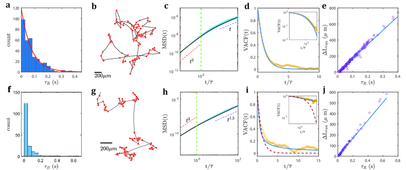
Figure 2: Top row: Run-and-tumble, Bottom row: Lévy walk; (a,f) distribution of run-time $\tau_{R}$ drawn from an exponential and power-law PDF. (b,g) trajectory of the Quincke walker performing a run-and-tumble and Lévy walk. (c,h) time-averaged mean-square displacement. Symbols: experiment, Solid line: theory, Vertical dashed line marks $\overline{\tau}$. (d,i) normalized velocity autocorrelation function, Symbols: experiment, Solid line: theory, dashed line -exponential decay. Inset: same in log-log scale plot. (e,j) Run length vs. the corresponding run time $\tau_{R}$. Symbols: experiment, Solid line: linear fit showing a constant run velocity of $V=1.73$ mm/s for Run-and-Tumble and $V=0.84$ m/s for Lévy walk. E$=1.83$ MV/m for run-and-tumble and E$=1.5$ MV/m for Lévy walks. For both run-and-tumble and Lévy walk: $\overline{\tau}=0.075$ s, $\tau_{T}/\tau_{{\mathrm{mw}}}=20$. $\gamma=1.7$ for Lévy walk.

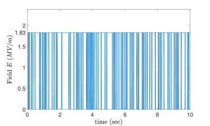
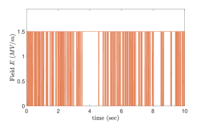
Figure 6: 10 second of the generated signal based on the exponential PDF of run-times $\tau_{R}$ for run-and-tumble motion (a) and power-law PDF for Lévy-walk (b).

We now proceed to construct more complex locomotion patterns such as run-and-tumble and Lévy walk. Unlike the simple random walk, which is characterized by a constant run time, run times for run-and-tumble motion are exponentially, and for Lévy walks – power-law, distributed. We randomly draw run times $\tau_{R}$ from the corresponding distribution $\psi_{R}$ (Fig. 2(a,f)) and encode this times as pulse durations in the electric signal (sample signals are shown in Fig. 6). In run-and-tumble, $\psi_{R}=1/\bar{\tau}e^{-t/\bar{\tau}}$, where $\bar{\tau}$ is the mean value for the run times Berg (2008); Angelani (2013). For Lévy walk with resting periods Zaburdaev et al. (2015), $\psi_{R}=\gamma t_{0}^{\gamma}t^{-(1+\gamma)}H(t-t_{0})$, where $\bar{\tau}=t_{0}\gamma/(\gamma-1)$ Sato et al. (1999); Angelani (2013). $H$ is the Heaviside function and $t_{0}$ is the lower cutoff value for run times. The power $1<\gamma<2$ controls the degree of anomalous super-diffusion manifested at long times. In both cases, we assume turning time $\tau_{T}$ and run velocity $V$ to be constant.

Sample trajectories of the Quincke roller performing a run-and-tumble motion and Lévy walk are shown in Fig. 2b,g. The measured mean squared displacement ( Fig. 2c,h) displays a transition from the initial ballistic regime for times shorter than $\overline{\tau}$ to final normal diffusion with a linear scaling with time in the case of run-and-tumble. The experimental results are in excellent agreement with the theoretical prediction Angelani (2013):

$$MSD(t)={2V^{2}\bar{\tau}^{2}}\left(e^{-t/\bar{\tau}}+t/\bar{\tau}-1\right)/{\left(1+\tau_{T}/\bar{\tau}\right)}\,.$$ (3)

The long-time MSD for Lévy walk exhibits superdiffusion with a power consistent with the theoretical scaling of $t^{3-\gamma}$. The experimentally observed superdiffusion persists up to $t/\overline{\tau}\approx 100$, beyond which, it starts to deviate from the asymptotic theoretical scaling due to the under-sampling of longer stretches which are responsible for the anomalous superdiffusive behavior. Contrary to previous cases, enhancing the long time statistics by repeating the experiments over several realizations is not trivial as the chance of losing the particle from the field of view during one of the long excursions is very high. In order to further analyze the performance of the Quincke random walker, we measure the experimental velocity auto-correlation function VACF from the trajectory analysis. Fig. 2d shows a sharp decay of the VACF in the case of run and tumble motion, in agreement with the theoretical predictions:

$$VACF(t)={V^{2}}e^{-t/\bar{\tau}}/\left({1+\tau_{T}/\bar{\tau}}\right)\,.$$ (4)

For Lévy walk, VACF exhibits a tail (Fig. 2i) which agrees well with the theoretical prediction for the Lévy walk and shows a poor fit to an exponential curve which drops sharply to zero. This, plus the fact that particle’s displacement follows the desired distribution, further corroborates that the walker undergoes a Lévy walk. The run length (Fig. 2e,j) shows linear dependence on the corresponding run times, which confirms that the walker runs at almost constant speed.

Collective dynamics: The Quincke random walkers exhibit rich collective dynamics, summarized in Fig. 3 for the case of a simple walk.

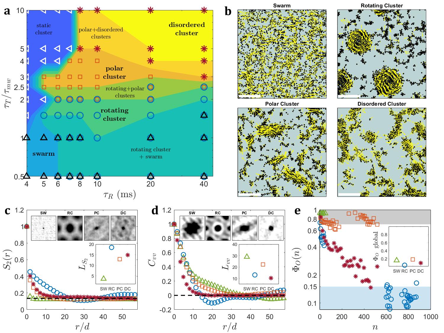
Figure 3: (a) Collective states formed by Quincke random walkers with different run and turn times ($\tau_{R}$, $\tau_{T}$). Symbols indicate the experimentally observed $\lhd$: static cluster, $\bigtriangleup$: swarm (SW), $\circ$: rotating cluster (RC), $\square$: polar cluster (PC), and $\ast$: disordered cluster (DC). (b) Snapshots of the SW ($\tau_{T}/\tau_{\mathrm{mw}}=0.5$,$\tau_{R}=4$ ms), RC ($\tau_{T}/\tau_{\mathrm{mw}}=1.5$,$\tau_{R}=5$ ms), PC ($\tau_{T}/\tau_{\mathrm{mw}}=3$,$\tau_{R}=8$ ms) and DC ($\tau_{T}/\tau_{\mathrm{mw}}=10$,$\tau_{R}=40$ ms) phases from the experiments. Scale bar is 1mm. Velocity vectors are superimposed to the particles. Particle area fraction and pulse amplitude are constant in all experiments and are equal to $\phi\approx 0.15$ and E$=2.08$ MV/m, respectively. (c) Angular-averaged normalized two-point correlation vs. radial distance $r$ normalized by particle diameter $d$; top inset: in 2D, showing the spatial periodicity of rotating cluster; bottom inset: characteristic length of two-point correlation functions defined as the point where $S_{2}$ crosses the horizontal line. (d) Angular-averaged velocity auto-correlation vs. normalized radial distance; top inset: in 2D, showing the periodicity of velocity correlation of rotating and polar clusters in space. Some degree of anisotropy in the velocity auto-correlation of polar cluster is due to insufficient number of clusters in the field of view; bottom inset: characteristic length of velocity auto-correlation functions, defined as the point where $C_{vv}$ crosses the zero line. (e) polar order parameter vs. cluster size of $n$ particle; inset: global order parameter, showing lack of any global ordering in all phases; shaded areas indicate polar ordering higher than $75\%$ and lower than $15\%$.

At a given particle density, depending upon the run time $\tau_{R}$ and the degree of depolarization $\tau_{T}/\tau_{\mathrm{mw}}$ (“memory”), the Quincke colloids self-organize into different dynamical phases at (statistically) steady-state with distinct statistical properties (Fig. 3c-e). The classical, run-only Quincke rollers Bricard et al. (2013) correspond to $\tau_{T}/\tau_{\mathrm{mw}}=0$. The phases are differentiated by examining the spatial two-point correlation function $S_{2}$, velocity auto-correlation function $C_{vv}$, and the polar order parameter $\Phi_{O}$ (see Appendix for definitions). The spatial correlations and order parameters are computed from equal-time averages over the frames corresponding to running periods. The flow field analysis in the population of particles was performed using an open source Matlab code PIVLab Thielicke and Stamhuis (2014).

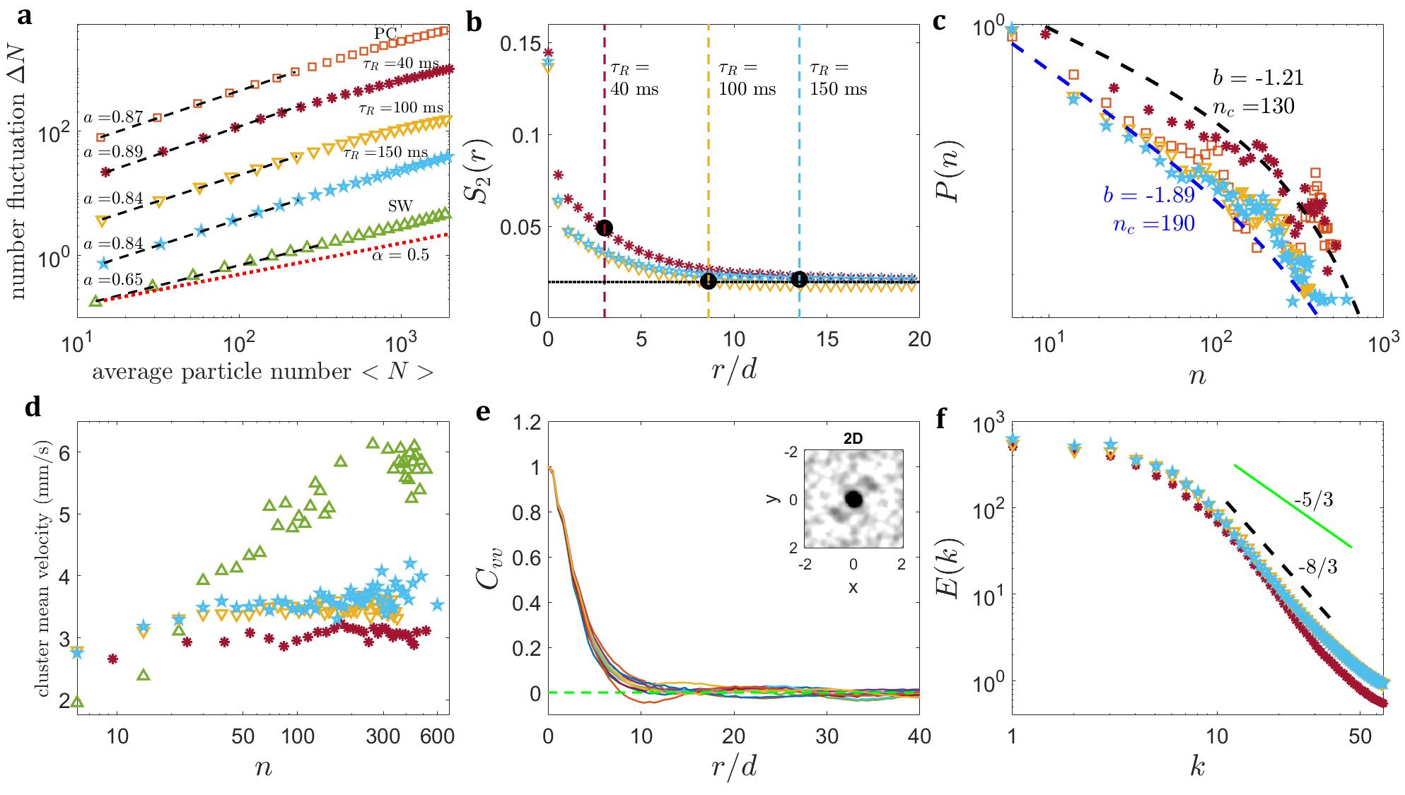
Figure 4: (a) Number fluctuations $\Delta N$ as a function of average number of particles $\langle N\rangle$. Normal fluctuation is shown by dotted line. Plots shifted vertically for better visualization. (b) Spatial two-point correlation of disordered clusters. Vertical lines depict the corresponding kinematic length scales. $\ast$:  ($\tau_{T}/\tau_{\mathrm{mw}}=10$,$\tau_{R}=40$ ms), $\triangledown$: ($\tau_{T}/\tau_{\mathrm{mw}}=10$,$\tau_{R}=100$ ms), $\star$: ($\tau_{T}/\tau_{\mathrm{mw}}=10$,$\tau_{R}=150$ ms). (c) Probability distribution of clusters with n number of particles (d) cluster mean velocity averaged over all the particles in a cluster as a function of cluster size of n. (e) Velocity auto-correlation of a disordered cluster with $\tau_{R}=100$ ms evaluated at different run steps. The anti-correlation around $r/d\approx 10$ shows the approximate size of the highly transient vortical structures formed in disordered clustering. Inset: All run-time averaged velocity auto-correlation in 2D. (f) Angular-averaged energy spectrum of disordered clusters formed by Quincke random walkers with different run times $\tau_{R}$= 40, 100 and 150 ms.
Symbols denote different phases: $\square$: polar cluster (PC) ($\tau_{T}/\tau_{\mathrm{mw}}=3$,$\tau_{R}=8$ ms), $\ast$: disordered cluster (DC)  ($\tau_{T}/\tau_{\mathrm{mw}}=10$,$\tau_{R}=40$ ms), $\triangledown$: disordered cluster ($\tau_{T}/\tau_{\mathrm{mw}}=10$,$\tau_{R}=100$ ms), $\star$: disordered cluster ($\tau_{T}/\tau_{\mathrm{mw}}=10$,$\tau_{R}=150$ ms), $\bigtriangleup$: swarm (SW) ($\tau_{T}/\tau_{\mathrm{mw}}=1$,$\tau_{R}=4$ ms)

If the colloid run directions are correlated due to significant memory effect ( $\tau_{T}/\tau_{\mathrm{mw}}<2$) and run times are short $\tau_{R}\sim\tau_{T}$, particles form swarms similar to those observed in Bricard et al. (2013, 2015). The fast-decay of $S_{2}$ in Fig. 3c and the corresponding characteristic length scale $L_{S_{2}}$ of a few particle diameter $d$, ($L_{S_{2}}$ defined as the length where $S_{2}$ crosses the horizontal line corresponding to the $r\rightarrow\infty$ limit), indicate lack of connectiveness or large scale clustering of the particles. However, swarms show long-range velocity correlations and high polar ordering, see Fig. 3d and e.

Increasing $\tau_{R}$, while keeping $\tau_{T}/\tau_{\mathrm{mw}}$ below 2, leads to the emergence of stable rotating cluster islands, with (periodic) long-range spatial pair and velocity correlations and very weak polar ordering (Fig. 3). It has been argued that pair-aligning interactions are responsible for local grouping of Quincke rollers in swarming state Bricard et al. (2013, 2015); Lu et al. (2018), however, recent particle-based simulations Großmann et al. (2015) suggest that the formation of rotating clusters can be attributed to the enhancement of a competing anti-aligning interaction.

As the memory effect fades, $\tau_{T}/\tau_{\mathrm{mw}}>2$, the swarm and rotating clusters disappear. At small to intermediate values of $\tau_{R}$, particles form stable large polar clusters, which cruise over the whole domain without significant exchange of particles. The main characteristic feature of these clusters is the long-range velocity and orientational order across giant moving clusters, as shown in Figs. 3(c-e).

As both $\tau_{T}$ and $\tau_{R}$ increase, the giant polar clusters break up by exchanging outermost particles, which start performing independent random-walks. This results in a more continuous spectrum of cluster size distribution at steady-state, with large clusters being orientationally decorrelated, as shown in Fig. 3e. The resulting disordered clusters are highly dynamic: they continuously evolve, deform and break by exchanging particles.

Clustering is characterized by anomalous density fluctuations (Fig. 4a). The particle number fluctuations $\Delta N$ scales with the average particle numbers $\langle N\rangle$ (in windows of different linear size) as $\Delta N\sim\langle N\rangle^{a}$, with exponent $a$ which is larger than the one for fluctuations observed for systems in thermal equilibrium $a=0.5$. Compared to the disordered and polar cluster phase, the swarming phase lacks long-range clustering, which results in a more uniform distribution of cells and thus a smaller power-law exponent $a$. The density fluctuations are sensitive to the run time. Fig. 4a shows that in the disordered cluster phase as $\tau_{R}$ increases from $40$ms to $100$ms and $150$ms, the power-law exponent $a$ decreases from $0.89$ to $0.84$. The origin can be traced to the relative magnitude of the Quincke roller average run length and the cluster size; if the run is shorter than the aggregate length, the particle remains trapped in the cluster. Fig.4b shows that the run length, estimated by the kinematic length scale of the random walkers $L_{k}=V\tau_{R}$, falls in regions with considerable degree of spatial correlation for the short run time $\tau_{R}=40$ms. However, for $\tau_{R}=100$ ms and $150$ ms, $L_{k}$ intersects the corresponding $S_{2}$ curves at points where spatial correlation almost vanishes. The longer kinematic length scale makes it possible for the outermost particles to leave their original cluster and diffuse into an already existing one or form a new cluster with other isolated random walkers. At even shorter run times, the kinematic length scale becomes much smaller than the pair-correlation length scale, which results in either very low mobility or even static clusters ((upper left part of the phase diagram in Fig. 3a))

Intriguingly, the observed anomalous scaling for the number density fluctuations in the polar and disordered cases are comparable with those obtained in moving clusters of gliding M. xanthus mutant Peruani et al. (2012) and swimming B. subtilis Zhang et al. (2010), thereby suggesting that the disordered clusters behave similarly to ones observed in bacterial systems. Indeed, the exponent of the inverse power-law scaling of the cluster size probability distribution (Fig. 4c), $P(n)\sim n^{b}e^{-n/n_{c}}$, agrees well with dynamic clustering in bacterial suspension and discrete particle simulations Zhang et al. (2010); Pohl and Stark (2014). Furthermore, as illustrated in Fig. 4d, cluster mean velocity $V_{m}$ increases with the size of the cluster and plateaus beyond certain cluster sizes, similar to Zhang et al. (2010). The figure also shows that the high orientational ordering in polar clusters significantly enhances the mean velocity, compared with the disordered clusters. The angular-averaged velocity auto-correlation of disordered clusters in Fig. 4e shows anti-correlation around $r/d\approx 10-20$, which is a signature for the formation of vortical structures, similar to those observed in different bacterial systems Dombrowski et al. (2004); Cisneros et al. (2007); Zhang et al. (2009); Cisneros et al. (2011); Wensink et al. (2012); Dunkel et al. (2013). The corresponding energy spectrum calculated from the velocity field of the particles shows scaling of $-8/3$ (see also Fig. 4f), which is in agreement with mesoscopic turbulence in bacterial suspension Wensink et al. (2012), discrete particle simulations Großmann et al. (2014), and also in numerical simulations for suspension of pushers in a Newtonian fluid Li and Ardekani (2016).

The quantitative similarity of the cluster and flow statistics of bacterial and Quincke walker clusters may originate from a unique feature of the Quincke random walkers: when the field is on, they all run and when the field is turned off, they all stop. This de facto synchronization of the runs and turns mimics physical locking and intertwining of flagella in dense clusters of bacterial systems and thus may play a role in the observed coordinated motionCopeland and Weibel (2009); Zhang et al. (2010).

The creation of the Quincke random walker enables the experimental study of active fluids emulating bacterial suspensions under well defined and controllable conditions, e.g., particle density, speed (i.e., activity) and walk type. In this work we only focused on the effects of the simple walk and its characteristics (run and turn times) on the collective dynamics at moderate particle density. Exploration of the complete phase space will likely discover more complex collective states, for example, preliminary results show vortex arrays similar to ones observed in swimming sperm Riedel et al. (2005) and in particle-based simulations Großmann et al. (2014, 2015). The Quincke random walker can also be programmed with alternating or time-varying speed Theves et al. (2013); Babel et al. (2014) and locomotions with distributed waiting times featuring anomalous subdiffusion. Another fundamental problem that can be investigated with the Quincke random walker is the navigation of biological microswimmers in the complex heterogeneous environment Morin et al. (2017a, b). This would provide an insight on how different search strategies, such as Lévy walk, are affected by the presence of obstacles and which intermittent motility pattern yields the optimal search strategy Zaburdaev et al. (2015); Volpe and Volpe (2017). Our approach can also be used to randomize the motion of other active particles powered by the Quincke effect such as the recently proposed helical propeller Das and Lauga (2019) and use this microswimmer to explore self-organization in three-dimensional suspensions.We envision the Quincke random walker as a new paradigm for active locomotion at the microscale and a testbed for the abundant theoretical models of the collective dynamics of active matter.

This research has been supported by NSF awards CBET-1704996 and CMMI-1740011.

Appendix A Quincke Effect

The spontaneous spinning of a rigid sphere in a uniform DC electric field $\mathbf{E}$ has been known for over a century Quincke (1896); Melcher and Taylor (1969); Lemaire and Lobry (2002). Yet this phenomenon has been largely overlooked until its recent application to power “active” particles, in particular the Quincke rollers Bricard et al. (2013, 2015); Snezhko (2016); Lavrentovich (2016); Pradillo et al. (2019).

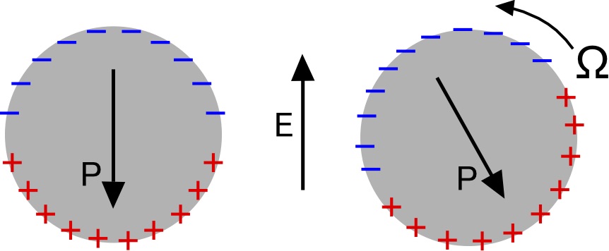
Figure 5: Induced free charge distribution for a sphere with $R/S<1$. Above a critical field strength $E>E_{Q}$ steady rotation around an axis perpendicular to the electric field is induced by the misaligned induced dipole of the particle (right). The rotation can be either clock- or counter-clockwise.

The phenomenon arises from particle polarization in an applied electric field due to the accumulation of free charges at the particle interface Melcher and Taylor (1969). The induced dipole due to these free charges lags the application of the uniform DC electric field as

$$\begin{split}{\bf{P}}=&\left(\chi_{0}-\chi_{\infty}\right){\bf E}\left[1-\exp\left(-t/t_{\mathrm{mw}}\right)\right]\,,\end{split}$$ (5)

where $\chi_{0},\,\chi_{\infty}$ are the low- and high-frequency susceptibilities of the particle, and $t_{{\mathrm{mw}}}$ is the Maxwell-Wagner polarization time. For a sphere with diameter $d$

$$\begin{split}\chi_{0}-\chi_{\infty}=\frac{\pi}{2}{\varepsilon}_{\mathrm{s}}d^{3}\frac{3(\mbox{\it R}-\mbox{\it S})}{(\mbox{\it R}+2)(\mbox{\it S}+2)}\,,\quad t_{{\mathrm{mw}}}=\frac{{\varepsilon}_{{\mathrm{p}}}+2{\varepsilon}_{{\mathrm{s}}}}{{\sigma}_{{\mathrm{p}}}+2{\sigma}_{{\mathrm{s}}}}\,.\end{split}$$ (6)

R and S characterize the mismatch of electrical conductivity ${\sigma}$, and permittivity ${\varepsilon}$, between the sphere and the suspending fluid:

$$\mbox{\it R}=\frac{{\sigma}_{\mathrm{p}}}{{\sigma}_{\mathrm{s}}}\,,\quad\mbox{\it S}=\frac{{\varepsilon}_{\mathrm{p}}}{{\varepsilon}_{\mathrm{s}}}\,,$$ (7)

where subscripts $``{\mathrm{p}}"$ and $``{\mathrm{s}}"$ denote values for the particle and suspending medium, respectively.

In order for rotation to occur, the induced free-charge dipole of the sphere should be oriented opposite to the direction of the applied field, which occurs when $\mbox{\it R}/\mbox{\it S}<1$ (see Eq. 5 and Eq. 6). This configuration is unfavorable and becomes unstable above a critical strength of the electric field. A perturbation tilts the dipole, leading to an electric torque that drives physical rotation of the sphere around an axis perpendicular to the applied field direction. For this rotation to be sustained, the rotation period should be comparable to the Maxwell-Wagner polarization time: this condition ensures that while the induced surface-charge distribution rotates with the sphere, the exterior fluid can recharge the interface by conduction. The balance between charge convection by rotation and supply by conduction from the bulk results in an oblique dipole orientation with a steady angle as shown in Figure 5.

The steady rotation rate $\Omega$ of the Quincke rotor is determined from conservation of angular momentum of the sphere, where electric and viscous torques balance rotational inertia Turcu (1987); Jones (1984); Lemaire and Lobry (2002):

$$\begin{split}I\frac{d\Omega}{dt}=P_{\perp}E-\zeta\Omega\,,\end{split}$$ (8)

Here, $I=\pi\rho_{\mathrm{p}}d^{5}/60$ is the moment of inertia and $\zeta=\pi\mu_{\mathrm{s}}d^{3}$ is the friction factor of the sphere. The dipole component orthogonal to the field direction, $P_{\perp}$, is determined from the coupled evolution equations for the polarization:

$$\begin{split}\frac{dP_{\perp}}{dt}&=-\Omega P_{||}-t_{\mathrm{mw}}^{-1}P_{\perp}\,,\\ \frac{dP_{||}}{dt}&=\Omega P_{\perp}-t_{\mathrm{mw}}^{-1}\left[P_{||}-\left(\chi_{0}-\chi_{\infty}\right)E\right]\,.\end{split}$$ (9)

The steady state solutions of Eq. 8 and Eq. 9 are no rotation ($\Omega=0$ with induced dipole $P_{||}$ given by Eq. 5 and $P_{\perp}=0$), and steady rotation with

$$\begin{split}\Omega&=\pm\frac{1}{t_{{\mathrm{mw}}}}\sqrt{\frac{E^{2}}{E_{Q}^{2}}-1}\,,\\ E_{Q}^{2}&=\frac{2{\sigma}_{\mathrm{s}}\mu_{\mathrm{s}}\left(\mbox{\it R}+2\right)^{2}}{3{\varepsilon}_{\mathrm{s}}^{2}(\mbox{\it S}-\mbox{\it R})}\,,\quad P_{\perp}=\frac{\zeta\Omega}{E}\,.\end{split}$$ (10)

where $\pm$ reflects the two possible directions of rotation, shows that rotation is only possible if the electric field exceeds a critical value given by $E_{Q}$.

Appendix B Experiment

The colloidal rollers are polystyrene spheres (Phosphorex, Inc.) with diameter $d=40\mu m$, density $\rho_{\mathrm{p}}=1.18$ g/cm³, and dielectric constant ${\varepsilon}_{\mathrm{p}}\sim 3$. The suspending fluid is hexadecane oil (Sigma Aldrich), density $\rho_{\mathrm{s}}$=0.77 g/cm³ and dielectric constant ${\varepsilon}_{\mathrm{s}}=2$ , containing 0.15 M AOT (Sigma Aldrich). The conductivity of the solution is $\sigma_{\mathrm{s}}=1.2\times 10^{-8}$ S/m, measured with a high-precision multimeter (BK Precision). The Maxwell-Wagner time for this system is $\tau_{\mathrm{mw}}\sim 2$ ms. The experimental setup consists of a $2\times 2$ cm² rectangular chamber made from two Indium-Tin-Oxide (ITO) coated glass slides (Delta Technologies) as electrodes, separated by a Teflon spacer with thickness 120 $\mu$m. The particle motion and tracking is visualized using an optical microscope (Zeiss) mounted on a vibration isolation table (Kinetic Systems, Inc.) and videos were recorded at frame rates higher than 500 frames per second by using a high speed camera (Photron). The waveform for each walk is programmed as a Matlab code and interfaced with a high voltage amplifier (Matsusada) through a function/wave generator (Agilent Technologies). Particle tracking and all analyses were performed using custom-written Matlab code. The flow field analysis in the population of particles was performed using an open source Matlab code PIVLab Thielicke and Stamhuis (2014).

Appendix C Quincke Random Walker vs. Active Brownian Particle

In order to compare the present Quincke random walker with active Brownian particles, we estimate the importance of Brownian translational and rotational diffusion by evaluating the Péclet number, $Pe=V/\sqrt{D_{T}\times D_{R}}$ Bechinger et al. (2016), where $D_{T}=k_{B}T/(3\pi\mu d)$ and $D_{R}=k_{B}T/(\pi\mu d^{3})$ are the Brownian translational and rotational diffusivities, and $k_{B}T$ is the thermal energy. For the particle and fluid system used in our experiments, the corresponding Réclet number is $Pe\approx 10^{6}$, implying that the Brownian diffusion can be ignored on the time scales of our experiments and that the rotational diffusion does not play any significant role in reorienting the Quincke random walker, in contrast to the artificial active Brownian particles.

The choice of particle size and the selected velocity range in this report are set by the limitations in the spatial and temporal resolutions of our experimental setup and a compromise for minimizing the localization error in single particle tracking. It is interesting to perform experiments where the contribution of Brownian diffusion is superposed on the run and turn events Thiel et al. (2012); Detcheverry (2017), similar to situations experienced by biological microswimmers. This can be achieved for example, through lowering the Péclet number by using smaller size particles, e.g. $1\mu m$, and lower velocities in the Quincke random walk.

Appendix D Theoretical MSD and VACF for individual random walkers

For any general run time distribution functions $\psi_{R}(t)$, we first compute the corresponding distributions in the Laplace domain, i.e. $\psi_{R}(s)$, and use the formulations presented in Angelani (2013); Detcheverry (2017) to find the mean-squared displacement $MSD(t)=\left\langle\left[{\bf x}(t+t^{\prime})-{\bf x}(t^{\prime})\right]^{2}\right\rangle$, where x is the position of the particle and the brackets denote time averaging with respect to the time variable $t^{\prime}$ for each trajectory. In all cases, we assume a constant run velocity $V$ and turning time $\tau_{T}$. Also, because the Péclet number for the Quincke random-walker is sufficiently high in all our experiments, we ignored the contribution from the Brownian diffusion in the theoretical MSD derivations.

For a random walk with a constant run time $\tau_{R}$, the corresponding distribution $\psi_{R}$ will be equal to $\psi_{R}(t)=\delta(t-\tau_{R})$, or equivalently $\psi_{R}(s)=e^{-s\tau_{R}}$ in the Laplace domain. Then, we find the mean-squared displacement as:

$$\begin{split}MSD(t)&=\frac{V^{2}}{3(\tau_{R}+\tau_{T})}\left[3\tau_{R}t^{2}-t^{3}\right]\quad\textrm{for $t<\tau_{R}$}\ \\ &=\frac{V^{2}}{3(\tau_{R}+\tau_{T})}\left[\tau_{R}^{2}(3t-\tau_{R})\right]\quad\textrm{for $t>\tau_{R}$}\ \end{split}$$ (11)

For the run-and-tumble motion with a mean run time $\overline{\tau}$, the run times are drawn from an exponential distribution $\psi_{R}(t)=1/\overline{\tau}\ e^{-t/\overline{\tau}}$, or equivalently $\psi_{R}(s)=1/(1+s\overline{\tau})$ in the Laplace domain. The mean-squared displacement is readily given by Angelani (2013); Detcheverry (2017):

$$MSD(t)=\frac{2\ V^{2}\ \overline{\tau}^{2}}{1+\tau_{T}/\overline{\tau}}\left[e^{-t/\overline{\tau}}+t/\overline{\tau}-1\right].$$ (12)

For the Lévy walk, we extract the run times from a power-law distribution of the form $\psi_{R}=\gamma\ t_{0}^{\gamma}\ t^{-(1+\gamma)}\ H(t-t_{0})$, where $H$ is the Heaviside function, $t_{0}$ is the lower cutoff for the run times, and $1<\gamma<2$ controls the extent of superdiffusive behavior of the walker that emerges at long times. The mean run time $\overline{\tau}$ becomes $\overline{\tau}=t_{0}\ \gamma/(\gamma-1)$. For $1<\gamma<2$, the mean-squared displacement is given by Angelani (2013):

$$\begin{split}MSD(t)&=\frac{V^{2}t^{2}}{(\overline{\tau}+\tau_{T})}\left[\overline{\tau}-t/3\right]\quad\textrm{for $t<t_{0}$}\ \\ &=\frac{V^{2}}{(\overline{\tau}+\tau_{T})}\left[\frac{\gamma t_{0}^{3}}{3(3-\gamma)}-\frac{\gamma t_{0}^{2}}{2-\gamma}t\right.\\ &\left.+\frac{2t_{0}^{\gamma}}{(\gamma-1)(2-\gamma)(3-\gamma)}t^{3-\gamma}\right]\quad\textrm{for $t>t_{0}$}\ \end{split}$$ (13)

To find the theoretical temporal velocity auto-correlation function $VACF(t)=\left\langle{\bf v}(t+t^{\prime})\cdot{\bf v}(t^{\prime})\right\rangle$, we use Eq. 11-Eq. 13 along with the relation d$MSD(t)$/d$t$ = $2\times\int VACF\ dt$. For the run-and-tumble motion with run times drawn from an exponential pdf, temporal VACF becomes:

$$VACF(t)=\frac{V^{2}}{1+\tau_{T}/\overline{\tau}}\ e^{-t/\overline{\tau}},$$ (14)

And for the Lévy walk with the power-law distribution of run times, we obtain the temporal VACF as:

$$\begin{split}VACF(t)&=\frac{V^{2}}{(\overline{\tau}+\tau_{T})}\left[\overline{\tau}-t\right]\qquad\textrm{for $t<t_{0}$}\ \\ &=\frac{V^{2}}{(\overline{\tau}+\tau_{T})}\left[\frac{t_{0}^{\gamma}}{(\gamma-1)}t^{1-\gamma}\right]\quad\textrm{for $t>t_{0}$}\ \end{split}$$ (15)

For calculating the experimental velocity auto-correlation function from the particle trajectory, we use the Wiener-Khinchin autocorrelation theorem Bracewell (1965). The experimental velocity auto-correlation then can be accurately calculated in the Fourier domain by taking the inverse Fourier Transform of $|FT({\bf v}(t))|^{2}$, i.e. absolute square of the Fourier transform $FT$ of the particle velocity v(t).

Appendix E Cluster identification, Spatial correlation functions and Order parameters

We define clusters as a group of all particles located at a distance closer than some threshold value, regardless of their orientation. Several trials show that binning based on a threshold distance of $1.4d-1.6d$, where $d$ is the diameter of a single colloid, would result in a correct identification of clusters.

The standard two-point correlation function $S_{2}$ provides a robust measure for calculating the probability of finding two points of a microstructure ${\bf x_{1}}$ and ${\bf x_{2}}$ both in the same phase, which for our purposes is the particle phase. It is defined as Torquato (2013):

$$S_{2}({\bf x_{1}},{\bf x_{2}})=<I({\bf x_{1}})\cdot I({\bf x_{2}})>,$$ (16)

where angular brackets denote an ensemble average over all possible pairs in space and $I$ is the indicator function or density phase field of the particle, having a value of 1 if it falls in particle and zero everywhere else. In case of a statistically isotropic system, $S_{2}({\bf x_{1}},{\bf x_{2}})$ van be angularly averaged to give $S_{2}(r)$, where the scalar $r$ is the distance between two points. The descriptor $S_{2}(r)$ contains a wealth of information regarding the connectivity of different phases in a microstructure. $S_{2}$ can be easily calculated using the Fourier transform of the binary field of each image. We take the average of $S_{2}$ from all the frames belonging to the running-period.

In order to extract the spatial (clustering) length scales of different patterns, we merge (bin) all the particles belonging to the same cluster and then compute $S_{2}$ for the binned binary image. This will provide an average cluster size that we observe in each dynamical pattern. The corresponding length scale $L_{S_{2}}$ is the point where $S_{2}$ curve starts to plateau. According to it’s definition in Eq. 16, $S_{2}(r=0)$ is equal to the particle volume fraction $\phi$ and $S_{2}(r\rightarrow\infty)$ will be equal to the joint probability of satisfying simultaneously $I({\bf x_{1}})=I({\bf x_{2}})=1$, which is $\phi^{2}$ Torquato (2013). We use both $S_{2}$ and normalized $S_{2}$, i.e. $S_{2}/S_{2}(r=0)$ interchangeably in our quantitative analysis.

The velocity auto-correlation $C_{vv}$ is calculated from the following relation:

$$C_{vv}({\bf x_{1}},{\bf x_{2}})=<{\bf v}(t,{\bf x_{1}})\cdot{\bf v}(t,{\bf x_{2}})>,$$ (17)

where angular brackets denote spatial averaging over all possible pairs. In case of a statistically isotropic system, we use the angular-averaged $C_{vv}(r)$, where $r$ is the distance between two points over the space. We use the normalized velocity auto-correlation in our analysis, i.e. $C_{vv}(r)/C_{vv}(r=0)$. From the velocity auto-correlation $C_{vv}({\bf x_{1}},{\bf x_{2}})$, we compute the 2D Fourier transform to get the energy spectrum $E_{2}(k_{x},k_{y})$, where $k_{x}$ and $k_{y}$ are wave-numbers in $x$ and $y$ directions, respectively. In case of a statistically isotropic field, we average $E(k_{x},k_{y})$ over different wave-number angles to get $E(k)$.

The order parameter $\Phi_{O}$ of a cluster containing $n$ particles is calculated from $\Phi_{O}=|<e^{i\theta}>|$, where $\theta$ is the instantaneous direction of motion of each particle in a cluster and $<.>$ is the average over all the particles in a specific cluster.

References

- Elgeti et al. [2015] J Elgeti, R G Winkler, and G Gompper. Physics of microswimmers – single particle motion and collective behavior: a review. Reports on Progress in Physics, 78(5):056601, 2015. URL http://stacks.iop.org/0034-4885/78/i=5/a=056601.
- Lauga [2016] Eric Lauga. Bacterial hydrodynamics. Annual Review of Fluid Mechanics, 48(1):105–130, 2016. doi: 10.1146/annurev-fluid-122414-034606. URL https://doi.org/10.1146/annurev-fluid-122414-034606.
- Berg and Brown [1972] Howard C. Berg and Douglas A. Brown. Chemotaxis in escherichia coli analysed by three-dimensional tracking. Nature, 239(7):500–504, 1972.
- Pilizota et al. [2009] Teuta Pilizota, Mostyn T. Brown, Mark C. Leake, Richard W. Branch, Richard M. Berry, and Judith P. Armitage. A molecular brake, not a clutch, stops the rhodobacter sphaeroides flagellar motor. Proceedings of the National Academy of Sciences, 106(28):11582–11587, 2009. ISSN 0027-8424. doi: 10.1073/pnas.0813164106.
- Theves et al. [2013] Matthias Theves, Johannes Taktikos, Vasily Zaburdaev, Holger Stark, and Carsten Beta. A bacterial swimmer with two alternating speeds of propagation. Biophysical Journal, 105(8):1915 – 1924, 2013. ISSN 0006-3495. doi: https://doi.org/10.1016/j.bpj.2013.08.047. URL http://www.sciencedirect.com/science/article/pii/S0006349513010217.
- Xie et al. [2011] Li Xie, Tuba Altindal, Suddhashil Chattopadhyay, and Xiao-Lun Wu. Bacterial flagellum as a propeller and as a rudder for efficient chemotaxis. Proceedings of the National Academy of Sciences, 108(6):2246–2251, 2011. ISSN 0027-8424. doi: 10.1073/pnas.1011953108.
- Ebbens and Gregory [2018] Stephen J. Ebbens and David Alexander Gregory. Catalytic janus colloids: Controlling trajectories of chemical microswimmers. Accounts of Chemical Research, 51(9):1931–1939, 2018. doi: 10.1021/acs.accounts.8b00243. URL https://doi.org/10.1021/acs.accounts.8b00243. PMID: 30070110.
- Han et al. [2018] Koohee Han, C. Wyatt Shields IV, and Orlin D. Velev. Engineering of self-propelling microbots and microdevices powered by magnetic and electric fields. Advanced Functional Materials, 28(25):1705953, 2018. doi: 10.1002/adfm.201705953. URL https://onlinelibrary.wiley.com/doi/abs/10.1002/adfm.201705953.
- Palagi and Fischer [2018] Stefano Palagi and Peer Fischer. Bioinspired microrobots. Nature Reviews Materials, 3(6):113–124, JUN 2018.
- Huang et al. [2019] H.-W. Huang, F. E. Uslu, P. Katsamba, E. Lauga, M. S. Sakar, and B. J. Nelson. Adaptive locomotion of artificial microswimmers. Science Advances, 5(1), 2019. doi: 10.1126/sciadv.aau1532. URL https://advances.sciencemag.org/content/5/1/eaau1532.
- Paxton et al. [2004] Walter F. Paxton, Kevin C. Kistler, Christine C. Olmeda, Ayusman Sen, Sarah K. St. Angelo, Yanyan Cao, Thomas E. Mallouk, Paul E. Lammert, and Vincent H. Crespi. Catalytic nanomotors:autonomous movement of striped nanorods. Journal of the American Chemical Society, 126(41):13424–13431, 2004. doi: 10.1021/ja047697z. PMID: 15479099.
- Fournier-Bidoz et al. [2005] S bastien Fournier-Bidoz, Andr C. Arsenault, Ian Manners, and Geoffrey A. Ozin. Synthetic self-propelled nanorotors. Chem. Commun., pages 441–443, 2005. doi: 10.1039/B414896G. URL http://dx.doi.org/10.1039/B414896G.
- Howse et al. [2007] Jonathan R. Howse, Richard A. L. Jones, Anthony J. Ryan, Tim Gough, Reza Vafabakhsh, and Ramin Golestanian. Self-motile colloidal particles: From directed propulsion to random walk. Phys. Rev. Lett., 99:048102, Jul 2007. doi: 10.1103/PhysRevLett.99.048102. URL https://link.aps.org/doi/10.1103/PhysRevLett.99.048102.
- Jiang et al. [2010] Hong-Ren Jiang, Natsuhiko Yoshinaga, and Masaki Sano. Active motion of a janus particle by self-thermophoresis in a defocused laser beam. Phys. Rev. Lett., 105:268302, Dec 2010. doi: 10.1103/PhysRevLett.105.268302. URL https://link.aps.org/doi/10.1103/PhysRevLett.105.268302.
- Buttinoni et al. [2012] Ivo Buttinoni, Giovanni Volpe, Felix K mmel, Giorgio Volpe, and Clemens Bechinger. Active brownian motion tunable by light. Journal of Physics: Condensed Matter, 24(28):284129, 2012. URL http://stacks.iop.org/0953-8984/24/i=28/a=284129.
- Baraban et al. [2013] Larysa Baraban, Robert Streubel, Denys Makarov, Luyang Han, Dmitriy Karnaushenko, Oliver G. Schmidt, and Gianaurelio Cuniberti. Fuel-free locomotion of janus motors: Magnetically induced thermophoresis. ACS Nano, 7(2):1360–1367, 2013. doi: 10.1021/nn305726m. PMID: 23268780.
- Samin and van Roij [2015] Sela Samin and René van Roij. Self-propulsion mechanism of active janus particles in near-critical binary mixtures. Phys. Rev. Lett., 115:188305, Oct 2015. doi: 10.1103/PhysRevLett.115.188305. URL https://link.aps.org/doi/10.1103/PhysRevLett.115.188305.
- Gomez-Solano et al. [2016] Juan Ruben Gomez-Solano, Alex Blokhuis, and Clemens Bechinger. Dynamics of self-propelled janus particles in viscoelastic fluids. Phys. Rev. Lett., 116:138301, Mar 2016. doi: 10.1103/PhysRevLett.116.138301. URL https://link.aps.org/doi/10.1103/PhysRevLett.116.138301.
- Narinder et al. [2018] N Narinder, Clemens Bechinger, and Juan Ruben Gomez-Solano. Memory-induced transition from a persistent random walk to circular motion for achiral microswimmers. Phys. Rev. Lett., 121:078003, Aug 2018. doi: 10.1103/PhysRevLett.121.078003. URL https://link.aps.org/doi/10.1103/PhysRevLett.121.078003.
- Ebbens et al. [2010] Stephen Ebbens, Richard A. L. Jones, Anthony J. Ryan, Ramin Golestanian, and Jonathan R. Howse. Self-assembled autonomous runners and tumblers. Phys. Rev. E, 82:015304, Jul 2010. doi: 10.1103/PhysRevE.82.015304.
- Ebbens et al. [2012] Stephen J. Ebbens, Gavin A. Buxton, Alexander Alexeev, Alireza Sadeghi, and Jonathan R. Howse. Synthetic running and tumbling: an autonomous navigation strategy for catalytic nanoswimmers. Soft Matter, 8:3077–3082, 2012. doi: 10.1039/C2SM07283A. URL http://dx.doi.org/10.1039/C2SM07283A.
- Mano et al. [2017] Tomoyuki Mano, Jean-Baptiste Delfau, Junichiro Iwasawa, and Masaki Sano. Optimal run-and-tumble–based transportation of a janus particle with active steering. Proceedings of the National Academy of Sciences, 114(13):E2580–E2589, 2017. ISSN 0027-8424. doi: 10.1073/pnas.1616013114.
- Celia Lozano and Bechinger [2018] Juan Ruben Gomez-Solano Celia Lozano and Clemens Bechinger. Run-and-tumble-like motion of active colloids in viscoelastic media. New J. Phys., 20:015008, 2018.
- Bricard et al. [2013] Antoine Bricard, Jean-Baptiste Caussin, Nicolas Desreumaux, Olivier Dauchot, and Denis Bartolo. Emergence of macroscopic directed motion in populations of motile colloids. Nature, 503:95–98, 2013.
- Bricard et al. [2015] Antoine Bricard, Jean-Baptiste Caussin, Debasish Das, Charles Savoie, Vijayakumar Chikkadi, Kyohei Shitara, Oleksandr Chepizhko, Fernando Peruani, David Saintillan, and Denis Bartolo. Emergent vortices in populations of colloidal rollers. Nature Communications, 6:7470, 2015.
- Pradillo et al. [2019 ] G. E. Pradillo, H. Karani, and Petia M. Vlahovska. Surface electroconvection instability. Soft Matter, :: 10.1039/c9sm01163c, 2019 .
- Quincke [1896] G. Quincke. Ueber rotation em im constanten electrischen felde. Ann. Phys. Chem., 59:417–86, 1896.
- Morin et al. [2017a] Alexandre Morin, David Lopes Cardozo, Vijayakumar Chikkadi, and Denis Bartolo. Diffusion, subdiffusion, and localization of active colloids in random post lattices. Phys. Rev. E, 96:042611, Oct 2017a. doi: 10.1103/PhysRevE.96.042611. URL https://link.aps.org/doi/10.1103/PhysRevE.96.042611.
- Geyer et al. [2018] Delphine Geyer, Alexandre Morin, and Denis Bartolo. Sounds and hydrodynamics of polar active fluids. Nature Materials, 17(9):789–793, SEP 2018. ISSN 1476-1122. doi: –10.1038/s41563-018-0123-4˝.
- Lemaire and Lobry [2002] E. Lemaire and L. Lobry. Chaotic behavior in electro-rotation. Physica A, 314(1-4):663–671, November 2002.
- Berg [2008] Howard C Berg. E. coli in Motion. Springer Science & Business Media, 2008.
- Angelani [2013] L. Angelani. Averaged run-and-tumble walks. EPL (Europhysics Letters), 102(2):20004, 2013. URL http://stacks.iop.org/0295-5075/102/i=2/a=20004.
- Zaburdaev et al. [2015] V Zaburdaev, S Denisov, and J Klafter. Lévy walks. Reviews of Modern Physics, 87(2):483, 2015.
- Sato et al. [1999] Ken-iti Sato, Sato Ken-Iti, and A Katok. Lévy processes and infinitely divisible distributions. Cambridge university press, 1999.
- Thielicke and Stamhuis [2014] William Thielicke and Eize J. Stamhuis. PIVlab – towards user-friendly, affordable and accurate digital particle image velocimetry in MATLAB. Journal of Open Research Software, 2, oct 2014. doi: 10.5334/jors.bl. URL https://doi.org/10.5334%2Fjors.bl.
- Lu et al. [2018] Shi Qing Lu, Bing Yue Zhang, Zhi Chao Zhang, Yan Shi, and Tian Hui Zhang. Pair aligning improved motility of quincke rollers. Soft Matter, 14:5092–5097, 2018.
- Großmann et al. [2015] R. Großmann, P. Romanczuk, M. Bär, and L. Schimansky-Geier. Pattern formation in active particle systems due to competing alignment interactions. The European Physical Journal Special Topics, 224(7):1325–1347, Jul 2015. ISSN 1951-6401. doi: 10.1140/epjst/e2015-02462-3. URL https://doi.org/10.1140/epjst/e2015-02462-3.
- Peruani et al. [2012] Fernando Peruani, Jörn Starruß, Vladimir Jakovljevic, Lotte Søgaard-Andersen, Andreas Deutsch, and Markus Bär. Collective motion and nonequilibrium cluster formation in colonies of gliding bacteria. Phys. Rev. Lett., 108:098102, Feb 2012. doi: 10.1103/PhysRevLett.108.098102. URL https://link.aps.org/doi/10.1103/PhysRevLett.108.098102.
- Zhang et al. [2010] H. P. Zhang, Avraham Beer, E.-L. Florin, and Harry L. Swinney. Collective motion and density fluctuations in bacterial colonies. Proceedings of the National Academy of Sciences, 107(31):13626–13630, 2010. ISSN 0027-8424. doi: 10.1073/pnas.1001651107. URL https://www.pnas.org/content/107/31/13626.
- Pohl and Stark [2014] Oliver Pohl and Holger Stark. Dynamic clustering and chemotactic collapse of self-phoretic active particles. Phys. Rev. Lett., 112:238303, Jun 2014. doi: 10.1103/PhysRevLett.112.238303. URL https://link.aps.org/doi/10.1103/PhysRevLett.112.238303.
- Dombrowski et al. [2004] Christopher Dombrowski, Luis Cisneros, Sunita Chatkaew, Raymond E. Goldstein, and John O. Kessler. Self-concentration and large-scale coherence in bacterial dynamics. Phys. Rev. Lett., 93:098103, Aug 2004. doi: 10.1103/PhysRevLett.93.098103. URL https://link.aps.org/doi/10.1103/PhysRevLett.93.098103.
- Cisneros et al. [2007] Luis H. Cisneros, Ricardo Cortez, Christopher Dombrowski, Raymond E. Goldstein, and John O. Kessler. Fluid dynamics of self-propelled microorganisms, from individuals to concentrated populations. Experiments in Fluids, 43(5):737–753, Nov 2007. ISSN 1432-1114. doi: 10.1007/s00348-007-0387-y. URL https://doi.org/10.1007/s00348-007-0387-y.
- Zhang et al. [2009] H. P. Zhang, Avraham Beer, Rachel S. Smith, E.-L. Florin, and Harry L. Swinney. Swarming dynamics in bacterial colonies. EPL (Europhysics Letters), 87(4):48011, aug 2009. doi: 10.1209/0295-5075/87/48011. URL https://doi.org/10.1209%2F0295-5075%2F87%2F48011.
- Cisneros et al. [2011] Luis H. Cisneros, John O. Kessler, Sujoy Ganguly, and Raymond E. Goldstein. Dynamics of swimming bacteria: Transition to directional order at high concentration. Phys. Rev. E, 83:061907, Jun 2011. doi: 10.1103/PhysRevE.83.061907. URL https://link.aps.org/doi/10.1103/PhysRevE.83.061907.
- Wensink et al. [2012] Henricus H. Wensink, Jörn Dunkel, Sebastian Heidenreich, Knut Drescher, Raymond E. Goldstein, Hartmut Löwen, and Julia M. Yeomans. Meso-scale turbulence in living fluids. Proceedings of the National Academy of Sciences, 109(36):14308–14313, 2012. ISSN 0027-8424. doi: 10.1073/pnas.1202032109. URL https://www.pnas.org/content/109/36/14308.
- Dunkel et al. [2013] Jörn Dunkel, Sebastian Heidenreich, Knut Drescher, Henricus H. Wensink, Markus Bär, and Raymond E. Goldstein. Fluid dynamics of bacterial turbulence. Phys. Rev. Lett., 110:228102, May 2013. doi: 10.1103/PhysRevLett.110.228102. URL https://link.aps.org/doi/10.1103/PhysRevLett.110.228102.
- Großmann et al. [2014] Robert Großmann, Pawel Romanczuk, Markus Bär, and Lutz Schimansky-Geier. Vortex arrays and mesoscale turbulence of self-propelled particles. Phys. Rev. Lett., 113:258104, Dec 2014. doi: 10.1103/PhysRevLett.113.258104. URL https://link.aps.org/doi/10.1103/PhysRevLett.113.258104.
- Li and Ardekani [2016] Gaojin Li and Arezoo M. Ardekani. Collective motion of microorganisms in a viscoelastic fluid. Phys. Rev. Lett., 117:118001, Sep 2016. doi: 10.1103/PhysRevLett.117.118001. URL https://link.aps.org/doi/10.1103/PhysRevLett.117.118001.
- Copeland and Weibel [2009] Matthew F Copeland and Douglas B Weibel. Bacterial swarming: a model system for studying dynamic self-assembly. Soft matter, 5(6):1174–1187, 2009.
- Riedel et al. [2005] Ingmar H Riedel, Karsten Kruse, and Jonathon Howard. A self-organized vortex array of hydrodynamically entrained sperm cells. Science, 309(5732):300–303, 2005.
- Babel et al. [2014] S Babel, B ten Hagen, and H Löwen. Swimming path statistics of an active brownian particle with time-dependent self-propulsion. Journal of Statistical Mechanics: Theory and Experiment, 2014(2):P02011, 2014. URL http://stacks.iop.org/1742-5468/2014/i=2/a=P02011.
- Morin et al. [2017b] Alexandre Morin, Nicolas Desreumaux, Jean-Baptiste Caussin, and Denis Bartolo. Distortion and destruction of colloidal flocks in disordered environments. Nature Physics, 13:63?67, 2017b.
- Volpe and Volpe [2017] Giorgio Volpe and Giovanni Volpe. The topography of the environment alters the optimal search strategy for active particles. Proceedings of the National Academy of Sciences, 114(43):11350–11355, 2017.
- Das and Lauga [2019] Debasish Das and Eric Lauga. Active particles powered by quincke rotation in a bulk fluid. Phys. Rev. Lett., 122:194503, May 2019. doi: 10.1103/PhysRevLett.122.194503. URL https://link.aps.org/doi/10.1103/PhysRevLett.122.194503.
- Melcher and Taylor [1969] J. R. Melcher and G. I. Taylor. Electrohydrodynamics - a review of role of interfacial shear stress. Annu. Rev. Fluid Mech., 1:111–146, 1969.
- Snezhko [2016] Alexey Snezhko. Complex collective dynamics of active torque-driven colloids at interfaces. Current Opinion Coloid and Interface Sci., 21(SI):65–75, FEB 2016. ISSN 1359-0294. doi: –10.1016/j.cocis.2015.11.010˝.
- Lavrentovich [2016] Oleg D. Lavrentovich. Active colloids in liquid crystals. Current Opinion in Colloid and Interface Sci., 21(SI):97–109, FEB 2016. ISSN 1359-0294. doi: –10.1016/j.cocis.2015.11.008˝.
- Turcu [1987] I. Turcu. Electric field induced rotation of spheres. J. Phys. A: Math. Gen., 20:3301–3307, 1987.
- Jones [1984] T. B. Jones. Quincke rotation of spheres. IEEE Trans. Industry Appl., 20:845–849, 1984.
- Bechinger et al. [2016] Clemens Bechinger, Roberto Di Leonardo, Hartmut Löwen, Charles Reichhardt, Giorgio Volpe, and Giovanni Volpe. Active particles in complex and crowded environments. REVIEWS OF MODERN PHYSICS, 88(4):045006, 2016.
- Thiel et al. [2012] Felix Thiel, Lutz Schimansky-Geier, and Igor M. Sokolov. Anomalous diffusion in run-and-tumble motion. Phys. Rev. E, 86:021117, Aug 2012. doi: 10.1103/PhysRevE.86.021117. URL https://link.aps.org/doi/10.1103/PhysRevE.86.021117.
- Detcheverry [2017] Fran çois Detcheverry. Generalized run-and-turn motions: From bacteria to Lévy walks. Phys. Rev. E, 96:012415, Jul 2017. doi: 10.1103/PhysRevE.96.012415. URL https://link.aps.org/doi/10.1103/PhysRevE.96.012415.
- Bracewell [1965] R. Bracewell. The Fourier Transform and Its Applications. McGraw-Hill, New York, 1965.
- Torquato [2013] S. Torquato. Random Heterogeneous Materials: Microstructure and Macroscopic Properties. Springer Science & Business Media, Berlin, 2013.