Quantum magnetoresistive $(hc/2e)/m$ periodic oscillations in a superconducting ring

Abstract

It was experimentally found that quantum magnetoresistive $hc/2e$ periodic oscillations of the Little-Parks type in a superconducting mesoscopic ring with decreasing temperature and increasing applied dc current are modified to the sum of harmonic $(hc/2e)/m$ periodic oscillations. Multiple Andreev reflection can be a possible cause of this effect.

I INTRODUCTION

In order that to describe a multiply connected superconductor pierced by a magnetic flux $\Phi$, F. London proposed c1 the concept of the superconducting fluxoid $\Phi^{\ast}$ defined as $\Phi^{\ast}=\Phi+(4\pi/c)\oint\lambda_{L}^{2}$ J${}_{s}d$s$\,=\Phi+(m^{\ast}c/e^{\ast})\oint$ v${}_{s}d$s (here $c$ is the velocity of light, $\lambda_{L}$ is the London penetration depth of the magnetic field, J_s is the density of the circulating superconducting current, v_s is the superconducting velocity, $m^{\ast}$ and $e^{\ast}$ are the effective mass and effective electric charge of the superconducting pair, respectively). A remarkable property of superconductivity is that the superconducting fluxoid $\Phi^{\ast}$ is quantized, that is, $\Phi^{\ast}=n(hc/e^{\ast})=n\Phi_{0}$ (where $n$ is an integer, $h$ is the Planck’s constant, $e^{\ast}=2e$, $e$ is the electron charge, $\Phi_{0}=hc/e^{\ast}=hc/2e$ is the superconducting magnetic flux quantum). Moreover, the found experimental value $e^{\ast}=2e$ confirms that the effective charge of the superconductor is $2e$. In particular, quantization fluxoid leads to quantum oscillations of superconducting circulating current and the superconducting critical temperature $T_{c}$ (the Little-Parks effect c2 ) depending on the axial magnetic field $B$ in a thin-walled superconducting cylinder pierced by the flux and biased with a very low direct current $I_{dc}$, at temperatures $T$ very close to $T_{c}$. The periods of these oscillations correspond to the superconducting magnetic flux quantum $\Phi_{0}=hc/2e$ through the average cross-sectional area of the cylinder $S$.

The Little-Parks effect was observed in cylinders with a small radius $r\approx\xi(T)/2$ (where $\xi(T)$ is a temperature-dependent superconducting coherence length) under conditions very close to the equilibrium state. Under conditions close to a nonequilibrium state (at low temperatures and high currents), some violations in the $hc/2e$ periodicity of quantum magnetoresistive oscillations as a function of the axial magnetic field were found in inhomogeneous doubly connected structures with a small cross-sectional area: superconducting loops c3 ; c4 , Au_0.7In_0.3 cylinders c5 and hybrid metal-normal Ag rings with superconducting Al mirrors c6 . Anomalous negative magnetoresistance (NMR) and the absence of quantum $hc/2e$ periodic $R(B)$ oscillations were detected in low fields at low temperatures and high currents c3 . Deviations from the $hc/2e$ periodicity of Little-Parks oscillations in low fields were found in c4 . In addition, the NMR and $hc/4e$ periodic $R(B)$ oscillations were observed in superconducting cylinders c5 and hybrid SNS structures c6 at low temperatures. The period of $hc/4e$ was explained by the appearance of a new minimum of the free energy at $\Phi$ $=$ $\Phi_{0}(n+1/2)$ due to the formation of a $\pi$-junction in the Au_0.7In_0.3 cylinder c5 and multiple Andreev reflection c6 .

Quantum oscillations in superconducting loops of a larger area under clearly nonequilibrium conditions (high currents and $T$ below $T_{c}$) are not practically studied. In rings with larger radii $r\approx 2\xi(T)$, the amplitude of quantum oscillations should be expected to be low due to the lower circulating superconducting current and due to the fact that not all the ring can switch from the superconducting state to the normal state and back with a change in $B$.

The study of quantum magnetoresistive oscillations in superconducting mesoscopic rings without weak links (or without tunnel junctions) is challenging, since such rings can work as a highly sensitive superconducting quantum interference device (SQUID) c7 and as a highly efficient magnetic-dependent ac voltage rectifier (if the ring has circular asymmetry) c8 ; c9 .

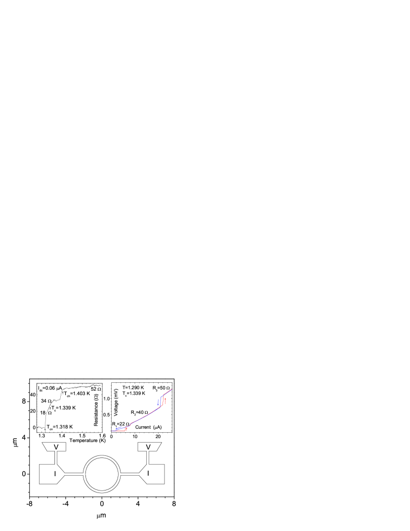
Figure 1: (Color online) The sketch of the structure. The letters $I$ and $V$ denote the current and potential wires. The left inset: Resistive $R(T)$ transition at $I_{dc}$ = $0.06$ $\mu$A. The right inset: $V(I)$ function at $T$ = $1.290$ K in the zero field; the arrows indicate the direction of the dc sweep.

It was found that periods of quantum magnetoresistive oscillations under strongly nonequilibrium conditions (at a high direct current $I_{dc}$ and $T$ below $T_{c}$)) can be $m$ times lower than the usual value and correspond to $\Phi_{0}/m$ $=$ $(hc/2e)/m$ ($m$ is an integer) through the effective area of the superconducting ring with a larger radius ($r=2$ $\mu$m $>\xi(T)$).

II SAMPLES AND EXPERIMENTAL PROCEDURE

$V(B)$ voltage was measured at different direct currents $I_{dc}>I_{c}$ at temperatures $T$ slightly below $T_{c}$ in superconducting mesoscopic structures (with close and different geometry), pierced by a magnetic flux. The structure under study (Fig. 1) was obtained by thermal evaporation of an aluminum film with a thickness of $d=51$ nm on a silicon substrate using the lift-off process of electron-beam lithography. The central region of the structure consists of a ring having a wall thickness $w_{r}$ = $0.27$ $\mu$m and an average radius $r_{m}$ = $1.94$ $\mu$m, narrow current $I$ wires with a width $w_{n}$ = $0.27$ $\mu$m, wide current wires with a width $w_{w}$ = $2$ $\mu$m and potential $V$ leads. Voltage $V$ was measured in the region including the ring, narrow $I$ wires and parts of wide $I$ wires (Fig. 1).

The structure had the parameters: resistance $R_{4.2K}=52.7$ $\Omega$ at $T=4.2$ K, resistance per square of film thickness $R_{sq}=\rho/d=1.97\,\Omega$, the ratio of resistances at $T=300$ K and 4.2 K is equal to $R_{300K}/R_{4.2K}=1.8$. The mean free path of quasiparticles $l=10$ nm was found from the refined theoretical c10 relation $\rho l=5.1\times 10^{-16}$ $\Omega$ $m^{2}$, where $\rho$ is the resistivity of the wire. The structure is a dirty superconductor, since $l<<\xi_{0}$ (where $\xi_{0}=1.6$ $\mu$m is the superconducting coherence length of pure aluminum at $T=0$ K). Near $T_{c}$ for the dirty case c11 , $\xi(T)=\xi(0)(1-T/T_{c})^{-1/2}$ (where $\xi(0)=0.85(\xi_{0}l)^{1/2}=0.11$ $\mu$m). The condition of quasi-one-dimensional superconductivity ($w_{n}$, $w_{r}<2\xi(T)$) is fulfilled near $T_{c}$. The nonequilibrium diffusion length of quasiparticles c3 ; c12 $\lambda_{Q}(T,I_{dc},B)=6-9$ $\mu$m near $T_{c}$. The structure has a length $L=10$ $\mu$m (the distance between $V$ leads), satisfying the condition $\xi(T)<<L<2\lambda_{Q}(T,I_{dc},B)$.

III RESULTS AND DISCUSSION

The resistive $R(T)$ transition of the structure from the normal (N) state to the superconducting (S) state is recorded at a direct current $I_{dc}$ = $0.06$ $\mu$A (the left inset of Fig. 1). The transition is rather stretched, which indicates the heterogeneity of the structure. The beginning of a sharp drop in $R(T)$ occurs at $T_{ch}$ = $1.403$ K and the resistance disappears at $T_{cn}=1.318$ K. The superconducting critical temperature $T_{c}$ = $1.339$ K is determined by the middle of the $R(T)$ transition. The contribution of the ring, expected from the geometry, to the total resistance of the structure is 23 $\Omega$. We assume that the upper segment of the $R(T)$ transition (from 52 to 18 $\Omega$) and the lower segment of $R(T)$ (from 18 to 0 $\Omega$) correspond to the NS transitions of the current wires and the ring, respectively. The function $V(I)$, recorded at $T$ = $1.290$ K, demonstrates phase current separation into sections with different resistance (the right inset of Fig. 1). The initial segment of the $V(I)$ function at low currents, including a nearly linear section with a resistance of 22 $\Omega$, characterizes SN (NS) transitions in the ring.

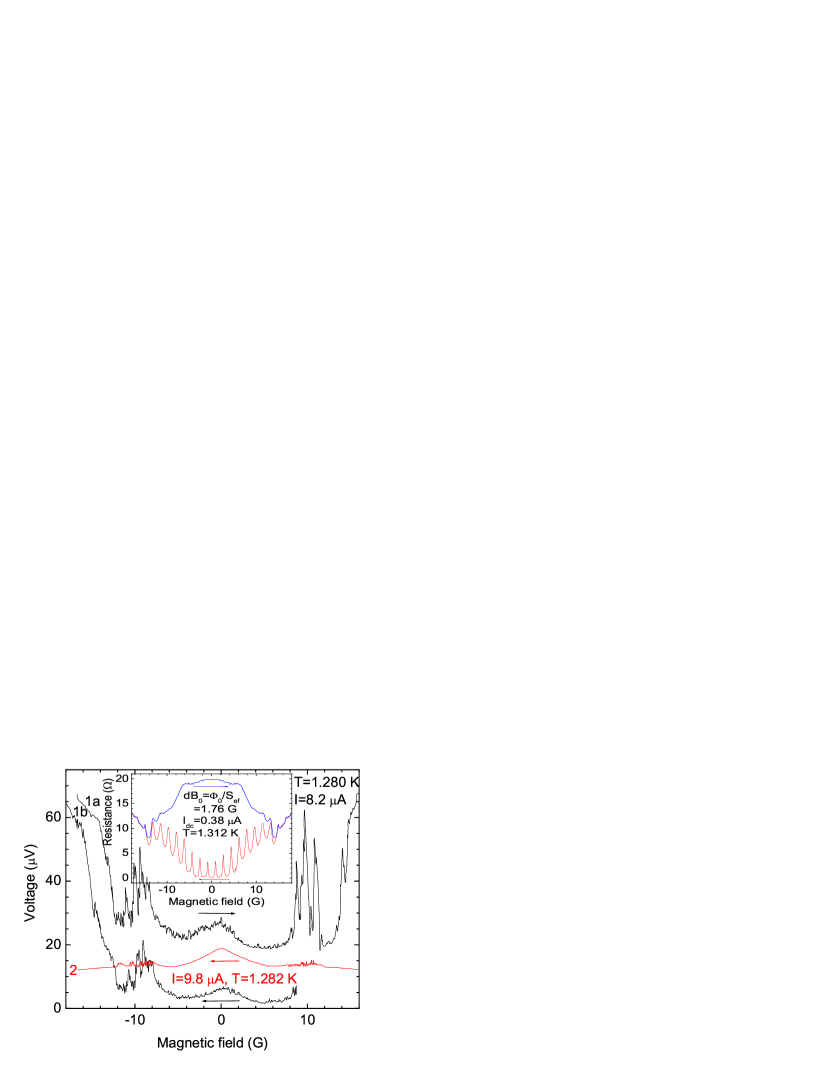
Figure 2: (Color online) $V(B)$ functions measured at $I_{dc}=8.2$ $\mu$A and $T=1.280$ K (curves 1a, 1b) and at $I_{dc}=9.8$ $\mu$A and $T=1.282$ K (curve 2). The arrows indicate the field sweep direction. The inset shows $V(B)$ function at $I_{dc}=0.38$ $\mu$A and $T=1.312$ K.

The magnetic field changed from a conditionally negative value of - 20 G to a conditionally positive value of + 20 G and back when measuring the $V(B)$ functions. In the field interval - 20, +20 G, only a part of the structure corresponding to the ring, switched into a resistive state with a resistance not exceeding $20$ $\Omega$ (Fig. 2 and the inset). The experimental $V(B)$ functions show an anomalous hysteresis depending on the direction of the field sweep (Fig. 2 and the inset). The ring has two states: a more dissipative state (the curve 1a of the Fig. 2 and the upper curve of the inset of Fig. 2) and a less dissipative state (the curves 1b,  2 of the Fig. 2 and the lower curve of the inset of Fig. 2). The causes of two states will be analyzed elsewhere. The considerable difference between two states is seen in the inset of Fig. 2.

The inset of Fig. 2 shows the $R(B)$ resistance as a function of the field, measured at a low current $I_{dc}$ = $0.06$ $\mu$A and $T$$\,=\,$1.312 K, very close to the bottom of the NS transition. The feature of the upper curve (the inset of Fig. 2) is the anomalous negative magnetoresistance (NMR), reaching a maximum at $B$ = $0$, equal to the ring resistance in the normal state. The anomalous dissipative state arises due to the thermodynamic fluctuations of the superconducting order parameter, leading to the formation of a phase slip center (PSC) c12 in the ring, despite the low current. Quantum magnetoresistive $hc/2e$ periodic oscillations of the Little-Parks type are visible on the lower curve (the inset of Fig. 2). The fundamental magnetic-field period of the oscillations is $dB_{0}$ = $\Phi_{0}/S_{eff}$ = $(hc/2e)/S_{eff}$ = $1.76$ G and corresponds to the superconducting magnetic flux quantum $\Phi_{0}$ = $hc/2e$ through the effective ring area $S_{eff}$. $S_{eff}$ almost coincides with the mean geometric area of the ring. The fundamental frequency $f_{0}$ = $dB_{0}^{-1}$ = $0.569$ G^-1 has the meaning of the reciprocal of the fundamental oscillation period $dB_{0}$.

The $V(B)$ functions recorded at lower $T$ = $1.280-1.284$ K and high currents $I_{dc}$ = $7.5-11$ $\mu$A also have a hysteresis decreasing with increasing $I_{dc}$. In addition, the curves 1a,  1b, and 2 of the Fig. 2 show anomalous negative magnetoresistance in two field intervals: fields close to zero and low fields. Figure 2 shows two of these unusual $V(B)$ functions measured at $I_{dc}$ = $8.2$ $\mu$A and $T=1.280$ K (curves 1a, 1b) and at $I_{dc}=9.8$ $\mu$A and $T$ = $1.282$ K (curve 2). The right segment of curve 1b and the upper curve, close to curve 2, recorded for the other direction of the field sweep, are not shown in Fig. 2.

Negative magnetoresistance appeared in a threshold manner at a certain current $I_{dc}>I_{r}$. Here $I_{r}$ is the retrapping superconducting critical current at which $V(I)$ on the structure disappears with decreasing $I_{dc}$. In addition, unusual $V(B)$ oscillations were found against the background of the NMR near the zero field at currents $I_{dc}$ = $1-3$ $\mu$A (not shown here) and low fields (6-12 G) at high currents $I_{dc}$ = $7.5-11$ $\mu$A (Fig. 2). Figure 3 shows the right segment of curve  2 (Fig. 2) measured several times and demonstrating unusual oscillations. These oscillations are not noise, they are almost reproducible when re-recording and differ slightly depending on the direction of the field sweep.

The Fourier spectrum of oscillations is usually calculated for a detailed analysis. The Fourier spectrum of any $x(t)$ oscillations, existing in a limited interval from $t_{1}$ to $t_{2}$, contains, besides the physical frequencies, fictitious frequencies: zero frequency and frequencies $f_{k}$ = $k$ $dt_{1,2}^{-1}$ (where $k$ is an integer, $dt_{1,2}$ = $t_{2}-t_{1}$ - interval length). Moreover, the physical frequencies can be shifted by the value of $k$ $dt_{1,2}^{-1}$. Fictitious low frequencies were observed in the spectra of the $V(B)$ functions in c9 ; c13 . It was found that for $V(B)$ oscillations (Fig. 3) the fundamental frequency $f_{0}$ is close in order of value to $dB_{1,2}^{-1}$ (here $dB_{1,2}$ = $B_{2}-B_{1}$ is the length of the oscillation existence interval), therefore distortions are expected in the Fourier spectrum.

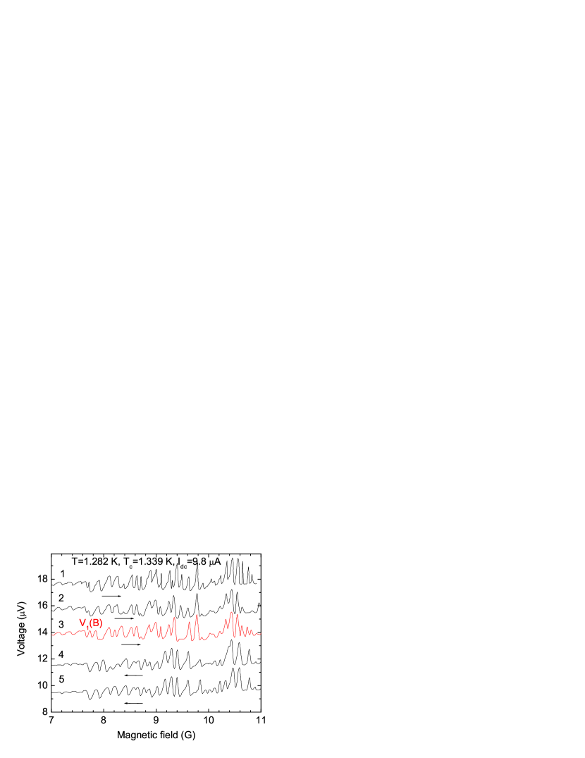
Figure 3: (Color online) $V(B)$ functions measured many times at $I_{dc}=9.8$ $\mu$A and $T=1.282$ K in the fields $B=7-11$ G. The arrows indicate the direction of the field sweep. The $V(B)$ functions, except $V_{1}(B)$ function (curve 3) are shifted vertically relative to the neighboring function by 2 $\mu$V.

In order to better see the distortions in the spectra, we plotted the Fourier transform (Figs. 4 - 6) of the $V(B)$ oscillations with the given interval lengths $dB_{1,2}=j$ $dB_{0}=j$ $f_{0}^{-1}$ (where $j=3$  and  1). The zero and fictitious frequencies $f_{k,j}=k$ $dB_{1,2}^{-1}=(k/j)dB_{0}^{-1}=(k/j)f_{0}^{-1}$ were expected to find in the spectrum, besides the physical frequencies. In addition, physical frequencies were expected to shift by $f_{k,j}$.

Fast Fourier transforms (FFTs) were obtained using 16384 evenly distributed points in given intervals of fields. So the condition $dB_{1,2}=B_{2}-B_{1}=11.36-6.09=3dB_{0}=3f_{0}^{-1}$ is fulfilled for the FFT spectrum of the $V_{1}(B)$ function (the curve 3 of Fig. 3) taken in the field interval from 6.09 to 11.36 G. This spectrum (Fig. 4) contains the fundamental frequency $f_{0}=dB_{0}^{-1}=S_{ef}/\Phi_{0}=0.569$ G^-1. The values of $f_{0}$ found from the period of the Little-Parks type oscillations (the inset of Fig. 2) and the spectrum (Fig. 4) coincide. In addition to $f_{0}$, the spectrum contains many higher harmonics of the fundamental frequency $f_{0}$, defined as $f_{m}=mf_{0}$ (where $m=2-20$). Some frequency peaks (Fig. 4) are shifted by 1/3, since the condition $dB_{1,2}=11.36-6.09=3dB_{0}=3f_{0}^{-1}$ is specified. All FFT spectra, including this spectrum (Fig. 4), contain a fictitious zero frequency. The contributions of the fundamental frequency and many higher harmonics to the spectrum are close. This indicates the presence of various fractional ($\Phi_{0}/m=(hc/2e)/m$) periods of $V_{1}(B)$ oscillations that are not a consequence of the inharmonicity of the $hc/2e$ oscillations. Some fractional $(hc/2e)/m$ magnetic flux periods, corresponding to fractional $dB_{0}/m$ magnetic field periods, are clearly distinguishable on the $V_{1}(B)$ function (the curve 3 of Fig. 3). Inharmonicity of oscillations is believed to make a very low contribution to the higher harmonics of the fundamental frequency $f_{0}$.

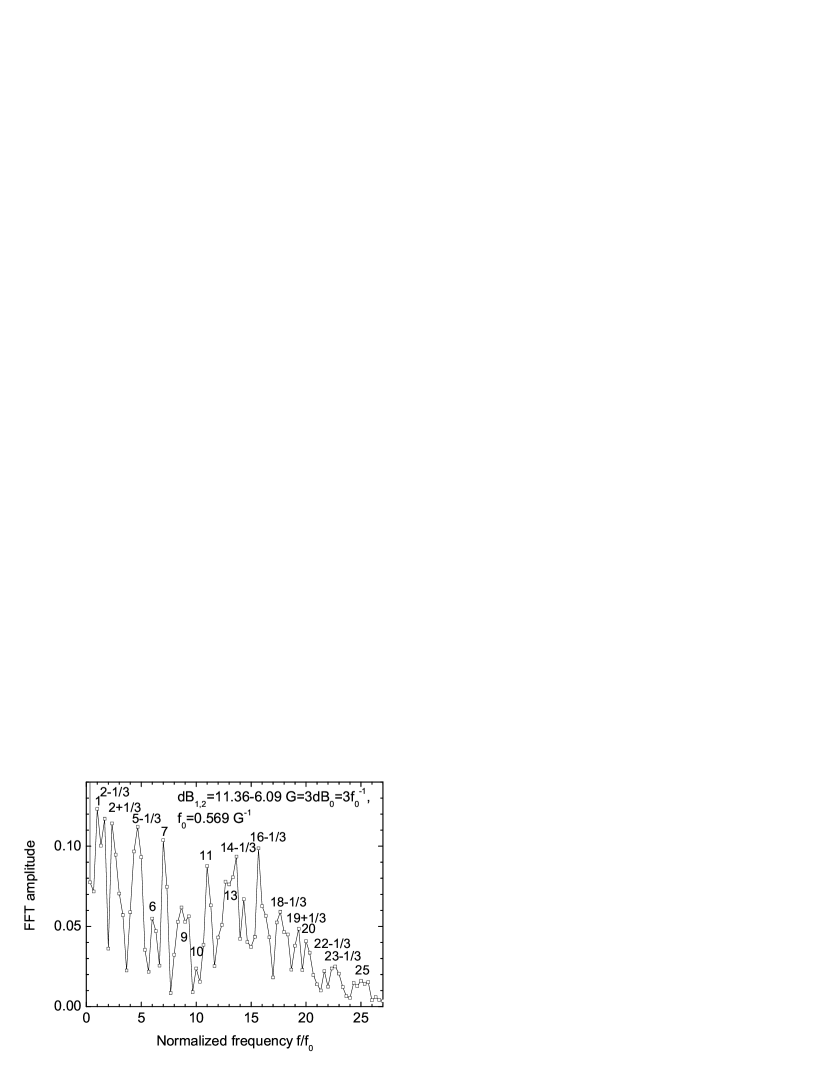
Figure 4: The FFT spectrum of the $V_{1}(B)$ function (the curve 3 of Fig. 3), taken in the interval of fields from $6.09$ to $11.36$ G. The condition $dB_{1,2}=11.36-6.09=3dB_{0}=3f_{0}^{-1}$ is satisfied.

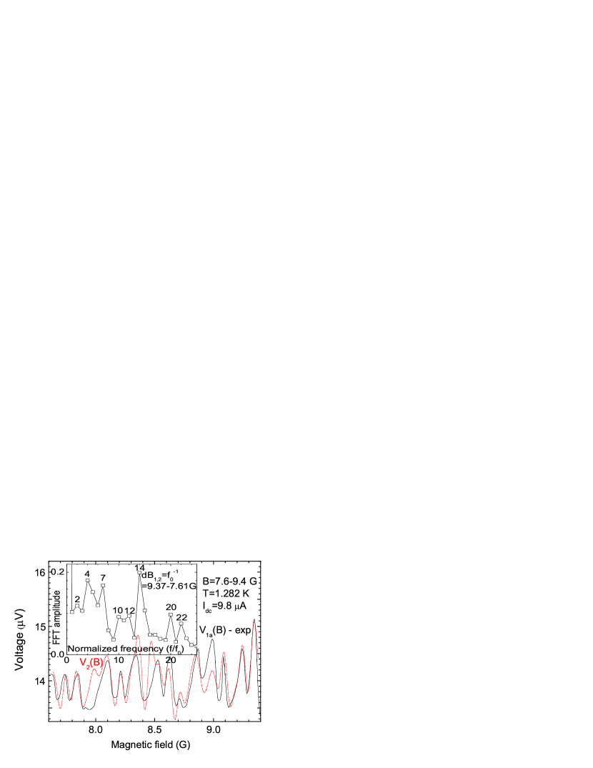
Figure 5: (Color online) The $V_{1a}(B)$ function (solid line) is part of the experimental $V_{1}(B)$ function (the curve 3 of Fig. 3), shown in fields $7.61$ - $9.37$ G; the $V_{2}(B)$ function (dash - dotted line) - qualitative fitting of the $V_{1a}(B)$ function. The inset: Fourier amplitude as a function of the normalized frequency $f/f_{0}$, obtained from the $V_{1a}(B)$ function in fields $7.61$ - $9.37$ G. The condition $dB_{1,2}$ = $9.37$ - $7.61$ = $dB_{0}$ = $f_{0}^{-1}$ is satisfied.

For a detailed analysis, the experimental $V_{1}(B)$ function (the curve 3 of Fig. 3) is divided into two functions $V_{1a}(B)$ in fields 7.6-9.4 G (Fig. 5) and $V_{1b}(B)$ in fields 9.24-10.6 G (Fig. 6). The FFT spectra of both $V_{1a}(B)$ and $V_{1b}(B)$ functions are calculated in two field intervals of 7.61-9.37 G and 9.26-11.02 G, respectively (the insets of Figs. 5  and  6). Unlike the spectrum (Fig. 4), the spectra (Figs. 5  and  6) do not contain peaks shifted in frequency, since the conditions $dB_{1,2}=B_{2}-B_{1}=9.37-7.61=dB_{0}=f_{0}^{-1}$ and $dB_{1,2}=11.02-9.26=dB_{0}=f_{0}^{-1}$ were specified. Certain numbers of $m$ dominate. The apparent absence of frequencies with other values of $m$ in the spectra, including $m=1$, is due to the low spectral resolution broadening the frequency peaks.

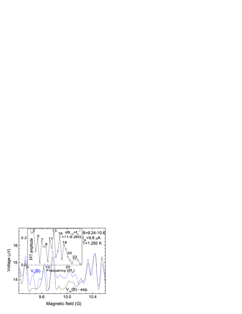
Figure 6: (Color online) $V_{1b}(B)$ function (solid line) is the part of the experimental $V_{1}(B)$ function (the curve 3 of Fig. 3), shown in fields $9.24$ - $10.6$ G; $V_{3}(B)$ function (dash-dotted line) is the qualitative fitting of the $V_{1b}(B)$ function. The inset: Fourier amplitude as a function of $f/f_{0}$, obtained from the $V_{1b}(B)$ function in fields $9.26$ - $11.02$ G. The condition $dB_{1,2}=11.02-9.26=dB_{0}=f_{0}^{-1}$ is fulfilled.

Only in order to qualitatively show that the $V_{1}(B)$ function really has a certain set of different oscillation periods, the different sections of $V_{1}(B)$ were approximated by fitting functions. The fitting has nothing to do with the theoretical description of the $V_{1}(B)$ oscillations. The expression $s+p\Sigma^{k}(a_{k}sin(2\pi mf_{0}B+\varphi_{k}))$, was used for the fitting, consisting of a constant shift $s$ and the multiplication of the coefficient $p\approx 1$ to the sum of sinusoidal oscillations with different amplitudes $a_{k}$, frequencies $mf_{0}$ and phases $\varphi_{k}$ that are multiples of $\pi/4$. The index $m$, corresponding to the harmonic number, took some integer values. The results of the spectra were taken into account (Figs. 5  and  6); therefore, $a_{k}$ are close to the Fourier amplitudes obtained from the spectra. Other options are available for fitting of the $V_{1}(B)$ function.

Two fitting functions $V_{2}(B)$ and $V_{3}(B)$ are used, respectively, for a qualitative description of $V_{1a}(B)$ (Fig. 5) and $V_{1b}(B)$ (Fig. 6) functions that are parts of the experimental $V_{1}(B)$ function. The prevalence in the spectra (the insets of Figs. 5  and  6) of certain frequencies $f_{m}$ = $mf_{0}$ (where $m$ = $2$, 4, 7, 10, 12, 14, 20, 22 for $V_{2}(B)$ and $m$ = $3$, 5, 7, 9, 11, 13, 16, 18 for $V_{3}(B)$) is taken into account. The functions of $V_{2}(B)$ and $V_{3}(B)$ are given below.

$V_{2}(B)=14.05+1.3(0.12sin(2\pi 2f_{0}B-\pi/2)+$

$+0.18sin(2\pi 4f_{0}B)+0.17sin(2\pi 7f_{0}B+\pi/4)+$

$+0.1sin(2\pi 10f_{0}B-\pi/4)+0.1sin(2\pi 12f_{0}B+\pi/2)+$

$+0.2sin(2\pi 14f_{0}B-\pi/2)+0.1sin(2\pi 20f_{0}B)+$

$+0.08sin(2\pi 22f_{0}B+3\pi/4))$.

$V_{3}(B)=14.3+1.25(0.245sin(2\pi 3f_{0}B+\pi)+$

$+0.2sin(2\pi 5f_{0}B-3\pi/4)+0.17sin(2\pi 7f_{0}B+\pi/4)+$

$+0.14sin(2\pi 9f_{0}B+\pi/4)+0.18sin(2\pi 11f_{0}B)+$

$+0.24sin(2\pi 13f_{0}B)+0.22sin(2\pi 16f_{0}B+\pi/2)+$

$+0.15sin(2\pi 18f_{0}B+3\pi/4))$.

The $V_{1c}(B)$ and $V_{1d}(B)$ functions that are parts of the experimental $V_{1}(B)$ function (the curve 3 of Fig. 3) are shown in Figures 7 and 8 with solid lines, approximations of short sections of both functions are shown with the broken lines. The short sections with the numbers 1 - 11 of the $V_{1c}(B)$ function (Fig. 7) and the sections 1 - 10 of the $V_{1d}(B)$ function (Fig. 8) are fitted by a single sinusoidal oscillation or a sum of several oscillations with different amplitudes, frequencies $f_{m}$ = $mf_{0}$ and phases.

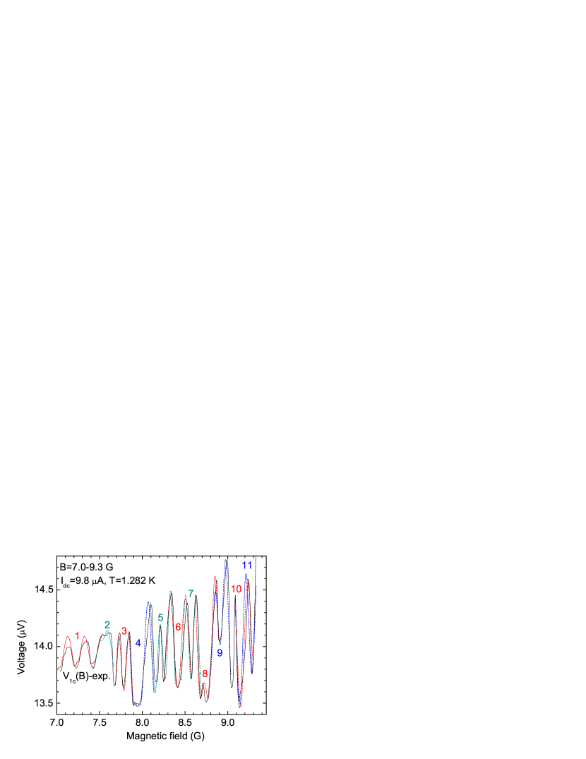
Figure 7: (Color online) $V_{1c}(B)$ function (solid line) is the part of the $V_{1}(B)$ function (the curve 3 of Fig. 3), shown in fields $7.0$ - $8.3$ G. The curves 1, 3, 5, 6, 8, 11 (dash-dotted lines) and 2, 4, 7, 9, 10 (dashed lines) are approximations of individual sections of the $V_{1c}(B)$ function with a set of fitting functions $F_{k}(B)$.

Sets of fitting functions $F_{k}(B)$ (Fig. 7) are described for the curves: 1 (in the fields 7.0-7.5 G), 2 (7.41-7.67 G), 3 (7.68-7.89 G), 4 (7.84-8.13 G), 5 (8.09-8.38 G), 6 (8.255-8.57 G), 7 (8.45-8.69 G), 8 (8.62-8.89 G), 9 (8.79-9.03 G), 10 (9.08-9.3 G), 11 (9.08-9.3 G) with the following expressions:

$F_{1}(B)=13.95+0.14sin(2\pi 9f_{0}B-\pi/2)$;

$F_{2}(B)=14+0.14sin(2\pi 7f_{0}B+\pi/4)+$

$+0.06sin(2\pi 14f_{0}B-3\pi/4)$;

$F_{3}(B)=13.8+0.1sin(2\pi 7f_{0}B+\pi/2)+$

$+0.29sin(2\pi 14f_{0}B-\pi/2)$;

$F_{4}(B)=13.8+0.45sin(2\pi 7f_{0}B+\pi/4)+$

$+0.15sin(2\pi 14f_{0}B)$;

$F_{5}(B)=14+0.16sin(2\pi 7f_{0}B+\pi/4)+$

$+0.34sin(2\pi 14f_{0}B-\pi/4)$;

$F_{6}(B)=14.03+0.39sin(2\pi 10f_{0}B-\pi/4)$;

$F_{7}(B)=14.0+0.1sin(2\pi 4f_{0}B-\pi/2)+$

$+0.39sin(2\pi 14f_{0}B-\pi)$;

$F_{8}(B)=13.9+0.47sin(2\pi 7f_{0}B)+$

$+0.25sin(2\pi 14f_{0}B-\pi/2)$;

$F_{9}(B)=14.25+0.2sin(2\pi 7f_{0}B-3\pi/4)+$

$+0.37sin(2\pi 14f_{0}B-\pi/2)$;

$F_{10}(B)=14.15+0.17sin(2\pi 7f_{0}B+\pi/2)+$

$+0.56sin(2\pi 12f_{0}B+3\pi/4)$;

$F_{11}(B)=14.05+0.25sin(2\pi 7f_{0}B+3\pi/4)+$

$+0.36sin(2\pi 12f_{0}B+\pi/2)$,

respectively. It can be seen that the oscillation frequencies used to approximate the short sections 1-11 of the $V_{1c}(B)$ function (Fig. 7) are as follows: $f=9f_{0}$ (section 1); $7f_{0}$ and 14$f_{0}$ (sections 2, 3, 4, 5, 8, 9); 10$f_{0}$ (section 6); 4$f_{0}$, and 14$f_{0}$ (section 7); $7f_{0}$, and $12f_{0}$ (sections 10, and 11).

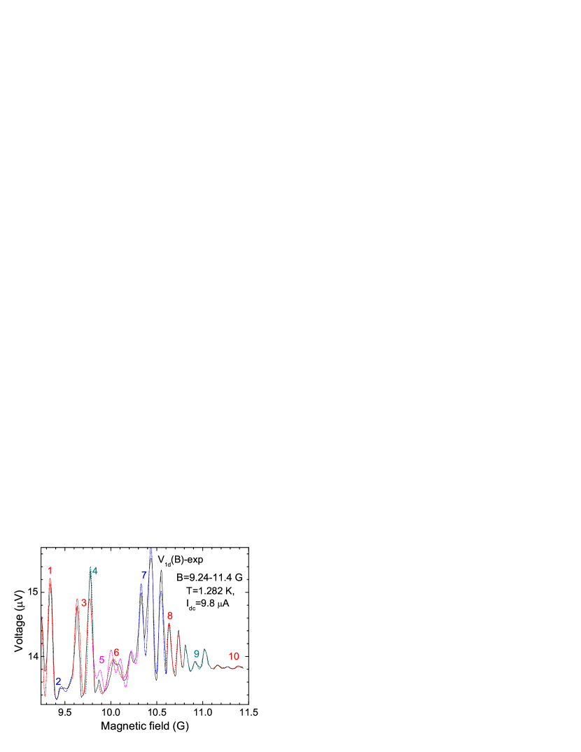
Figure 8: (Color online) $V_{1d}(B)$ function (solid line) is the part of the $V_{1}(B)$ function (the curve 3 of Fig. 3), shown in fields $9.24$ - $11.4$ G. The curves 1, 3, 5, 7, 9, 10 (dash-dotted lines) and 2, 4, 6, 8 (dashed lines) are approximations of individual sections of the $V_{1d}(B)$ function with a set of fitting functions $A_{k}(B)$.

The fitting functions $A_{k}(B)$ (Fig. 8) are described for the curves: 1 ($B=9.25-9.4$ G), 2 (9.38-9.58 G), 3 (9.58-9.83 G), 4 (9.73-9.83 G), 5 (9.8-10.3 G), 6 (9.9-10.2 G), 7 (10.3-10.6 G), 8 (10.6-10.77 G), 9 (10.81-11.06 G), 10 (11.12-11.44 G) with the following expressions:

$A_{1}(B)=14.3+0.92sin(2\pi 16f_{0}B+\pi/2)$;

$A_{2}(B)=13.565+0.135sin(2\pi 5f_{0}B-\pi/4)+$

$+0.15sin(2\pi 16f_{0}B)+0.1sin(2\pi 18f_{0}B-3\pi/4)$;

$A_{3}(B)=14.15+0.75sin(2\pi 13f_{0}B)$;

$A_{4}(B)=14.4+sin(2\pi 16f_{0}B+\pi/2)$;

$A_{5}(B)=13.9+0.85(0.24sin(2\pi 3f_{0}B-3\pi/4)+$

$+0.19sin(2\pi 5f_{0}B-3\pi/4)+0.17sin(2\pi 7f_{0}B+3\pi/4)+$

$+0.22sin(2\pi 16f_{0}B+\pi/2))$;

$A_{6}(B)=13.78+1.1(0.2sin(2\pi 5f_{0}B+3\pi/4)+$

$+0.3sin(2\pi 7f_{0}B+3\pi/4))$;

$A_{7}(B)=14.6+1.2(0.3sin(2\pi 7f_{0}B-\pi/2)+$

$+0.65sin(2\pi 16f_{0}B+\pi/2))$;

$A_{8}(B)=14.05+1.1(0.16sin(2\pi 11f_{0}B+\pi)+$

$+0.4sin(2\pi 16f_{0}B+\pi))$;

$A_{9}(B)=13.9+1.2(0.077sin(2\pi 9f_{0}B-\pi/4)$+

$+0.097sin(2\pi 16f_{0}B-\pi/4))$;

$A_{10}(B)=13.83+1.2(0.009sin(2\pi 7f_{0}B-\pi/2)+$

$+0.015sin(2\pi 16f_{0}B-3\pi/4))$,

respectively. The oscillation frequencies used to fit the sections 1 - 10 of the $V_{1d}(B)$ function (Fig. 8) are as follows: $16f_{0}$ (section 1); $5f_{0}$, $16f_{0}$ and $18f_{0}$ (section 2); $13f_{0}$ (section 3); $16f_{0}$ (section 4); $3f_{0}$, $5f_{0}$, $7f_{0}$ and $16f_{0}$ (section 5); $5f_{0}$ and $7f_{0}$ (section 6); $7f_{0}$ and $16f_{0}$ (section 7); $11f_{0}$ and $16f_{0}$ (section 8); $9f_{0}$ and $16f_{0}$ (section 9); $7f_{0}$ and $16f_{0}$ (section 10).

The detailed analysis, including the Fourier transform of $V(B)$ oscillations (the curve 2 of Fig. 2 measured at $I_{dc}$ = $9.8\mu$A and $T$ = $1.282$ K in fields 6-12 G) has been done. It can be seen from the FFT spectrum (Fig. 4) that the contributions of the fundamental frequency $f_{0}$ and the majority of higher harmonics $f_{m}$ = $mf_{0}$ ($m$ = $2-20$) to the spectrum are close. Each of the remaining higher harmonics makes a contribution that is approximately two times lower than the contribution of $f_{0}$.

In addition, other unusual experimental $V(B)$ oscillations were measured in low fields of 6-12 G at $T$ = $1.280-1.284$ K (not presented here). The maximum oscillation amplitude decreased from 25 $\mu$V to 0 with an increase in the current $I_{dc}$ from 7.5 to 11 $\mu$A. Thus, this amplitude reached 20 and 2 $\mu$V at currents of 8.2 and 9.8 $\mu$A (Fig. 2), respectively. At currents $I_{dc}$ = $7.7-8.6$ $\mu$A, the contributions of higher harmonics $f_{m}$ = $mf_{0}$ ($m$ = $3-20$) to the spectra (not presented here) were close, but approximately two times less than the contributions of frequencies $f_{0}$ and $2f_{0}$.

Previously, negative magnetoresistance near $B\,=\,0$ was measured in superconducting quasi-one-dimensional wires with cross-sectional narrowing and in rings of small radii with inhomogeneities c3 . Quantum magnetoresistive oscillations in the anomalous region of the NMR were not detected in c3 . Two regions of negative magnetoresistance (near the zero field and in the low fields) were found.

A generally accepted mechanism of NMR has not been proposed so far. The negative magnetoresistance in our structure can be due to a decrease in the resistance of the nonequilibrium SN boundary $R_{Q}\approx\lambda_{Q}(T,I_{dc},B)$ with the increasing field c3 . Another reason for the NMR can be an increase in the retrapping superconducting critical current $I_{r}$ and a decrease in the resistance of the structure (restoring of superconductivity) at a given current with the increasing field due to a decrease in the ”effective temperature” of hot quasiparticles in a non-equilibrium region of the structure c14 . The ”effective temperature” decreases due to an increase in the diffusion of overheated quasiparticles into neighboring superconducting banks with a slightly larger value of the superconducting order parameter $\Delta(T,B)$, when $\Delta(T,B)$ in superconducting banks decreases (or is completely suppressed) with the increasing field c14 .

The non-equilibrium region is the phase slip center or the SNS junction, in the center of which $\Delta(T,B)$ it periodically becomes zero and has a time-averaged non-zero value lower than in neighboring superconducting regions c12 . Oscillations of the order parameter give rise to a large quantity of hot quasiparticles, leading to a strong heating of the nonequilibrium region. The multiple Andreev reflection (MAR) c15 ; c16 ; c17 , occurring in the phase slip center or the SNS junction at voltages lower than the superconducting gap, increases the quasiparticle heating. The heating is enhanced due to the large electron-phonon relaxation time in the aluminum structure. Superconductivity and dissipation coexist in the non-equilibrium region c18 .

Although the theory c14 is valid only for short samples with a distance between potential leads $L$ = $5\xi(T)<2\lambda_{Q}(T,I_{dc},B)$. It can qualitatively explain the NMR of the experimental $V(B)$ functions in our structure with an average length $L$ = $20\xi(T)$ = $10$  $\mu$m, satisfying the condition $2\xi(T)<<L<2\lambda_{Q}(T,I_{dc},B)$. We assume that both the NMR regions in the fields close to the zero and in low fields are due to the formation of a superconducting barrier for diffusion of hot quasiparticles at the transition point of a narrow current wire to the wide current wire.

This superconducting barrier is significantly weakened (or disappears) in a low field $B_{b}(T,I_{dc})$, dependent on $T$ and $I_{dc}$. The value $B_{b}(T,I_{dc})$ is close to the third critical field $B_{c3}(T)$ at low currents. The appearance of superconductivity along the boundary of a wide current wire becomes impossible in the fields above $B_{c3}(T)$. The critical field $B_{c3}(T)\approx 2B_{c2}(T)$ is estimated for the point of transition of narrow current wires to wide current wires. Multiplier 2 is taken due to the wedge-shaped transitions c19 . For the $V(B)$ function (the inset of Fig. 2), the calculated value $B_{c3}(T=1.312K)\approx 2\Phi_{0}/2\pi\xi(T)^{2}\approx 12$  G is close to the experimental value of the field at which the negative magnetoresistance disappears ($B$ = $14$ G). For the $V(B)$ function (the curve 2 of Fig. 2), $B_{c3}(T=1.282K)\approx 22-26$ G was greater than the field at which the NMR disappears ($B$ = $12$ G), since the effect of the large direct current $I_{dc}$ is not taken into account. We believe that two regions of the NMR are due to several transitions between the diamagnetic and paramagnetic states of wide current wires with a change in the field. In the measurement, the maximum critical field $B_{max}(T)$ is not reached, at which superconductivity in narrow current wires and the ring is completely suppressed c11 . $B_{max}(T)$ = $77$ G at the temperature $T$ = $1.282$ K.

It is common knowledge that quantum magnetoresistive fractional $(hc/2e)/m$ (with $m>2$) periodic oscillations were not observed. We believe that oscillations with periods corresponding to $\Phi_{0}/m=(hc/2e)/m$ (where $m$ = $1-20$) and approximately equal amplitudes (except amplitude corresponding to $m=1$) indicate that the superconducting circulating current has effective charge $e^{\ast}=2em$. This phenomenon can be caused by the multiple Andreev reflection c15 ; c16 ; c17 ; c18 occurring in non-equilibrium regions of the structure (SNS junction or phase slip center formed in the ring) at voltages $V(I_{dc})<2\Delta(T,B)/e$. Here $\Delta(T,B)=\Delta(T)(1-(B/B_{max}(T))^{2})^{1/2}$ is the superconducting gap in the magnetic field $B$ at $T$ slightly below $T_{c}$. Where $\Delta(T)=3.07kT_{c}\Delta(0)(1-T/T_{c})^{1/2}$ is the gap at $B=0$ c11 . For the $V(B)$ function (the curve 2 of Fig. 2), $\Delta(T=1.282K,B=6-12G)=74-73$ $\mu$V.

It is known that multiple Andreev reflection can be realized in SNS junctions both in the ballistic case with the mean free path of quasiparticles $l$ greater than the length $l_{n}$ of the normal region of the junction c15 and in the diffusive case $(l<<l_{n})$ c16 ; c17 ; c18 . In this work, a diffusive the phase slip center or SNS junction is formed ($l<<l_{n}$ = $2\xi(T))$. To observe a large number of $n$ MAR in diffusive SNS junctions, it is required that the inelastic scattering length $l_{in}$ c16 (in our case, $l_{in}$ = $2\lambda_{Q}(T,I_{dc},B)$ = $12-18$ $\mu$m) is much larger than $l_{n}$. In this work, this requirement, written as $l_{in}$ = $2\lambda_{Q}(T,I_{dc},B)>>l_{n}$ = $2\xi(T)$, is satisfied.

In the process of multiple Andreev reflections, a quasi-electron (quasi-hole) with a energy smaller than the superconducting gap, located between two NS interfaces, is reflected as a quasi-hole (quasi-electron) alternately from both NS interfaces until it reaches the energy $V(I_{dc})en$ = $2\Delta(T,B)$. As a result of $n$ reflections, superconducting pairs in an amount equal to $m$ = $n/2$ or $m$ = $(n/2)-1$ appear in the superconducting region of the SNS junction or the phase slip center. Thus, the effective superconducting charge increases by a factor of $m$. The probability of observing MAR usually decreases with an increase in the number of reflections $n$, but from the experiment c18 it follows that MAR can be observed for a large number of reflections (up to $n$ = $32$). In c18 , it was found that MAR and very strong quasiparticle heating in the core of the phase slip center or SNS junction, formed in a quasi-one-dimensional superconducting aluminum wire, cause an appearance of current singularities in the form of a plateau on curves $V(I)$ at voltages $V_{pl,n}(T,B)$ = $2\Delta(T,B)/ne$, corresponding to the subharmonics of the superconducting gap. Here $n$ is a certain integer dependent on $T$,  $B$  and  $V$.

The ratio $2\Delta(T,B)/eV_{n}(I_{dc})\approx 146/14\approx 10$ shows the possible average MAR number for the $V(B)$ function (the curve 2 of Fig. 3). We assume that the maximum value of this ratio can be greater. It is expected that the instantaneous voltage $V(I_{dc})$ will vary from a value close to zero to a value close to the maximum voltage $V_{n}(I_{dc})$ = $20$ $\Omega$ $\times(I_{dc})\approx 160-200$ $\mu$V due to the presence of two different (less and more dissipative) states at currents $I_{dc}$ = $8-10$ $\mu$A. Therefore, the number of reflections can vary from one to the maximum possible value $2\lambda_{Q}(T,I_{dc},B)/\xi(T)\approx 18-36$.

IV CONCLUSION

We have found that a superconducting mesoscopic aluminum ring, pierced by a magnetic flux and biased with a direct current $I_{dc}$ at $T$ slightly below $T_{c}$, can be in two different (less or more dissipative) states.

The appearance of a certain state depends on the direction of the field sweep. Quantum magnetoresistive $hc/2e$ periodic oscillations of the Little-Parks type are observed in a less dissipative state at $T$, corresponding to the lowest $R(T)$ transition, and low $I_{dc}$ currents. In this case, $hc/2e$ oscillations are not found in the more dissipative state and the $V(B)$ function shows negative magnetoresistance. At lower $T$ and higher $I_{dc}$, both parts of the $V(B)$ function, corresponding to both dissipative states, exhibit two NMR regions (near $B$ = $0$ and in low fields). These NMR regions arise due to the formation of a superconducting barrier in wide current wires, which prevents the overheated region of the structure from cooling and non-monotonically depends on the field. Unusual quantum $V(B)$ oscillations can be observed in both NMR regions.

For the first time fractional $(hc/2e)/m$ (where $m=2-20$) periodic $V(B)$ oscillations have been studied in low fields. These oscillations were not described theoretically and measured previously. The decrease in the oscillation period by a factor of $m$ can be interpreted as an increase in the effective charge of the Cooper pairs by a factor of $m$, which occurs as a result of multiple Andreev reflections in the phase slip center or SNS junction formed in the ring.

The functions $V(B)$, measured in other structures, also show two dissipative states, the negative magnetoresistance and fractional $(hc/2e)/m$ periodic oscillations. At the same time, the amplitude corresponding to the fundamental oscillation period greatly exceeded the amplitudes corresponding to fractional periods.

V ACKNOWLEDGMENTS

This work was supported by the Ministry of Education and Science of the Russian Federation in the framework of State Assignment #075-00475-19-00. The authors thank V. Tulin, D. Vodolazov, V. Lukichev, A. Melnikov for the discussions and S. Dubonos for making structures.

References

- (1) F. London, Phys. Rev. 74, 562 (1948).
- (2) W. A. Little and R. D. Parks, Phys. Rev. Lett. 9, 9 (1962).
- (3) P. Santhanam, C. P. Umbach, and C. C. Chi, Phys. Rev. B 40, 11392 (1989).
- (4) H. Vloeberghs, V. V. Moshchalkov, C. Van Haesendonck, R. Jonckheere, and Y. Bruynseraede, Phys. Rev. Lett. 69, 1268 (1992).
- (5) Y. Zadorozhny and Y. Liu, Europhys. Lett. 55, 712 (2001).
- (6) V. T. Petrashov, V. N. Antonov, P. Delsing, and Claeson, Phys. Rev. Lett. 70, 347 (1993).
- (7) A. Barone and G. Paterno. Physics and Application of the Josephson Effect. John Willey and Sons, New York, 1982.
- (8) S.V. Dubonos, V.I. Kuznetsov, I.N. Zhilyaev, A.V. Nikulov, A.A. Firsov, JETP Letters 77, 371 (2003) (original Russian text: S.V. Dubonos, V.I. Kuznetsov, I.N. Zhilyaev, A.V. Nikulov, A.A. Firsov, Pis’ma v Zhurnal Eksperimental’noi i Teoreticheskoi Fiziki 77, 439 (2003)), https://doi.org/10.1134/1.1581963, arXiv:cond-mat/0303538.
- (9) V. I. Kuznetsov, A. A. Firsov, S. V. Dubonos, Phys. Rev. B 77, 094521 (2008), https://doi.org/10.1103/PhysRevB.77.094521.
- (10) M. Gershenson and W. L. McLean, J. Low Temp. Phys. 47, 123 (1982).
- (11) V. V. Schmidt, The Physics of Superconductors (Eds. P. Muller, A. Ustinov, Springer-Verlag, Berlin-Heidelberg, 1997).
- (12) R. Tidecks, Current-Induced Nonequilibrium Phenomena in Quasi-One-Dimensional Superconductors, Springer Tracts in Modern Physics, vol. 121, Springer-Verlag, Berlin-Heidelberg, 1990.
- (13) V. I. Kuznetsov, A. A. Firsov, Physica C 492, 11 (2013), https://doi.org/10.1016/j.physc.2013.05.003.
- (14) D. Y. Vodolazov, and F. M. Peeters, Phys. Rev. B 85, 024508 (2012).
- (15) M. Octavio, M. Tinkham, G. E. Blonder, and T. M. Klapwijk, Phys. Rev. B 27, 6739 (1983).
- (16) A. Bardas and D. V. Averin, Phys. Rev. B 56, R8518 (1997).
- (17) E. V. Bezuglyi, E. N. Bratus’, V. S. Shumeiko, G. Wendin, and H. Takayanagi, Phys. Rev. B 62, 14439 (2000).
- (18) V. I. Kuznetsov, A. A. Firsov, JETP Lett. 104, 709 (2016) (original Russian text: V. I. Kuznetsov, A. A. Firsov, Pis’ma v Zhurnal Eksperimental’noi i Teoreticheskoi Fiziki 104, 721 (2016)), https://doi.org/10.1134/S0021364016220100.
- (19) V. A. Schweigert and F. M. Peeters, Phys. Rev. B 60, 3084 (1999).