Prediction in regression models with continuous observations

Abstract

We consider the problem of predicting values of a random process or field satisfying a linear model $y(x)=\theta^{\top}f(x)+\varepsilon(x)$, where errors $\varepsilon(x)$ are correlated. This is a common problem in kriging, where the case of discrete observations is standard. By focussing on the case of continuous observations, we derive expressions for the best linear unbiased predictors and their mean squared error. Our results are also applicable in the case where the derivatives of the process $y$ are available, and either a response or one of its derivatives need to be predicted. The theoretical results are illustrated by several examples in particular for the popular Matérn $3/2$ kernel.

Keywords: Optimal prediction; correlated observations; kriging; best linear unbiased estimation

AMS Subject Classification: Primary 62M20; 60G25;

1 Introduction

A common problem, which occurs in many different areas, most notably geostatistics (Ripley, 1991; Cressie, 1993), computer experiments (Sacks et al., 1989; Stein, 1999; Santner et al., 2003; Leatherman et al., 2017) and machine learning (Rasmussen and Williams, 2006), is to predict the response $y(t_{0})$ at a point $t_{0}\in\mathbb{R}^{d}$ from given responses $y(t_{1}),\ldots,y(t_{N})$ at points $t_{1},\ldots,t_{N}\in\mathbb{R}^{d}$, where $t_{0}\neq t_{i}$ for all $i=1,\ldots,N$. Making the prediction assuming that responses are observations of a random field is called kriging (Stein, 1999). In classical kriging, it is assumed that $y$ is a random field of the form

$$y(t)=f^{\top}(t)\theta+\epsilon(t),$$ (1.1)

where $f(t)\in\mathbb{R}^{m}$ is a vector of known regression functions, $\theta\in\mathbb{R}^{m}$ is a vector of unknown parameters and $\epsilon$ is a random field with zero mean and existing covariance kernel, say $K(t,s)=E[\epsilon(t)\epsilon(s)]$. The components of the vector-function $f(t)$ are assumed to be linearly independent on the set of points where the observations have been made.

It is well-known, see e.g. Sacks et al. (1989), that in the case of discrete observations the best linear unbiased predictor (BLUP) of $y(t_{0})$ has the form

$$\hat{y}(t_{0})=f^{\top}(t_{0})\hat{\theta}_{\mathrm{BLUE}}+K^{\top}_{t_{0}}\Sigma^{-1}(Y-X\hat{\theta}_{\mathrm{BLUE}}),$$ (1.2)

where $\Sigma=\big{(}K(t_{i},t_{j})\big{)}_{i,j=1}^{N}$ is an $N\!\times\!N$-matrix, $K_{t_{0}}=\big{(}K(t_{0},t_{1}),\ldots,K(t_{0},t_{N})\big{)}^{\top}$ is a vector in $\mathbb{R}^{N}$, $X=(f(t_{1}),\ldots,f(t_{N}))^{\top}$ is an $N\!\times\!m$-matrix, $Y=(y(t_{1}),\ldots,$ $y(t_{N}))^{\top}\in\mathbb{R}^{N}$ is a vector of observations and

$$\hat{\theta}_{\mathrm{BLUE}}=(X^{\top}\Sigma^{-1}X)^{-1}X^{\top}\Sigma^{-1}Y$$

is the best linear unbiased estimator (BLUE) of $\theta$. The BLUP satisfies the unbiased condition $\mathbb{E}[\hat{y}(t_{0})]=\mathbb{E}[y(t_{0})]$ and minimizes the mean squared error $\mathrm{MSE}(\tilde{y}(t_{0}))=\mathbb{E}\left(y(t_{0})-\tilde{y}(t_{0})\right)^{2}$ in the class of all linear unbiased predictors $\tilde{y}(t_{0})$; its mean squared error is

$$\mathrm{MSE}(\hat{y}(t_{0}))=K(t_{0},t_{0})-\left[\begin{matrix}f(t_{0})\\ K_{t_{0}}\end{matrix}\right]^{\top}\left[\begin{matrix}0&X^{\top}\\ X&\Sigma\end{matrix}\right]^{-1}\left[\begin{matrix}f(t_{0})\\ K_{t_{0}}\end{matrix}\right].$$

In the present paper, we generalize the predictor (1.2) to the case of continuous observations of the response including possibly derivatives and prediction of derivatives and weighted averages of $y(t)$. We shall separately consider the cases where the observation region is an interval or a product set (in particular, square).

An important observation concerning construction of the BLUPs at different points is the fact that there is a considerable common part related to the use of the same BLUE. This could lead to significant computational savings relative to independent construction of the BLUPs. This observation extend to the cases when the observations are taken in $\mathbb{R}^{d}$ and when derivatives are also used for predictions.

The remaining part of this paper is organized as follows. In Section 2 we consider the BLUPs when we observe the process or field only. In Section 3 we study the BLUPs for either process values or one of its derivatives when we observe the process (or field) with derivatives. In Section 4 we provide proofs of the main results and in an Appendix we give more illustrating examples of the BLUPs for particular kernels.

2 Prediction without derivatives

2.1 Prediction at a point

Assume $\mathcal{T}\subset\mathbb{R}^{d}$ and consider prediction at a point $t_{0}\not\in\mathcal{T}$ for a response given by the model (1.1), where the observations for all $t\in\mathcal{T}$ are available. The vector-function $f\!:\mathcal{T}\!\to\!\mathbb{R}^{m}$ is assumed to contain functions which are bounded, integrable, smooth enough and linearly independent on $\mathcal{T}$; the covariance kernel $K(t,s)=E[\epsilon(t)\epsilon(s)]$ is assumed strictly positive definite.

A general linear predictor of $y(t_{0})$ can be defined as

$$\hat{y}_{Q}(t_{0})=\int_{\mathcal{T}}y(t)Q(dt),$$

where $Q$ is a signed measure defined on the Borel field of $\mathcal{T}$. This predictor is unbiased if $\mathbb{E}[\hat{y}_{Q}(t_{0})]=\mathbb{E}[y(t_{0})]$, which is equivalent to the condition

$$\int_{\mathcal{T}}f(t)Q(dt)=f(t_{0}).$$

The mean squared error (MSE) of $\hat{y}_{Q}(t_{0})$ is given by

$$\mathrm{MSE}(\hat{y}_{Q}(t_{0}))=\mathbb{E}\left(y(t_{0})-\hat{y}_{Q}(t_{0})\right)^{2}\,.$$

The best linear unbiased predictor (BLUP) $\hat{y}_{Q_{*}}(t_{0})$ of $y(t_{0})$ minimizes the mean squared error $\mathrm{MSE}(\hat{y}_{Q}(t_{0}))$ in the set of all linear unbiased predictors. The corresponding signed measure $Q_{*}$ will be called BLUP measure throughout this paper. Unlike the case of discrete observations, the BLUP measure does not have to exist for continuous observations.

Assumption A.

(1) The best linear unbiased estimator (BLUE) $\hat{\theta}_{\mathrm{BLUE}}=\int_{\mathcal{T}}y(t)G(dt)$ exists in the model (1.1), where $G(dt)$ is some signed vector-measure on $\mathcal{T}$,
(2) There exists a signed measure $\zeta_{t_{0}}(dt)$ which satisfies the equation

$$\int_{\mathcal{T}}K(t,s)\zeta_{t_{0}}(dt)=K(t_{0},s),\;\;\forall s\in\mathcal{T}.$$ (2.1)

Assumption A will be discussed in Section 2.2 below. We continue with a general statement establishing the existence and explicit form of the BLUP.

Theorem 2.1.

If Assumption A holds then the BLUP measure $Q_{*}$ exists and is given by

$$Q_{*}(dt)=\zeta_{t_{0}}(dt)+c^{\top}G(dt),$$ (2.2)

where the signed measure $\zeta_{t_{0}}(dt)$ satisfies (2.1) and $c=f(t_{0})-\int_{\mathcal{T}}f(t)\zeta_{t_{0}}(dt)\,.$ The MSE of the corresponding BLUP $\hat{y}_{Q_{*}}(t_{0})$ is given by

$$\mathrm{MSE}(\hat{y}_{Q_{*}}(t_{0}))=K(t_{0},t_{0})+c^{\top}Df(t_{0})-\int_{\mathcal{T}}K(t,t_{0})Q_{*}(dt)\,,$$ (2.3)

where $D=\int_{\mathcal{T}}\!\!\int_{\mathcal{T}}K(t,s)G(dt)G^{\top}(ds)$ is the covariance matrix of $\hat{\theta}_{\mathrm{BLUE}}=\int_{\mathcal{T}}y(t)G(dt)$.

This theorem is a particular case of a more general Theorem 2.2, which considers the problem of predicting an integral of the response. A few examples illustrating applications of Theorem 2.1 for particular kernels are given in the Appendix.

We can interpret the construction of the BLUP at $t_{0}$ in model (1.1) as the following two-stage algorithm. At stage 1, we use the BLUE $\hat{\theta}_{\mathrm{BLUE}}=\int_{\mathcal{T}}y(t)G(dt)$ for estimating $\theta$. At stage 2, we compute the BLUP in the model

$$\tilde{y}(t)=y(t)-f^{\top}(t)\widehat{\theta}_{BLUE}={\varepsilon}(t)-f^{\top}(t){\int_{\mathcal{T}}{\varepsilon}(t^{\prime})G(dt^{\prime})}\,,$$

which is a model with new error process and no trend. Straightforwardly, the covariance function of the process $\tilde{y}(t)$ is calculated as

$$\tilde{K}(t,s)=K(t,s)-f^{\top}(t)Df(s).$$

It then follows from Theorem 2.1 applied to the new model that the signed measure $Q_{*}(dt)$ satisfies the equation

$$\int_{\mathcal{T}}\tilde{K}(t,s)Q_{*}(dt)=\tilde{K}(s,t_{0}),\;\;\forall s\in\mathcal{T}\,.$$

From (2.3) in the new model, we obtain an alternative representation for the MSE of the BLUP $\hat{y}_{Q_{*}}(t_{0})$; that is,

$$\mathrm{MSE}(\hat{y}_{Q_{*}}(t_{0}))=\tilde{K}(t_{0},t_{0})-\int_{\mathcal{T}}\tilde{K}(t,t_{0})Q_{*}(dt)\,.$$

2.2 Validity of Assumption A

If ${\cal T}$ is a discrete set then Assumption A is satisfied for any strictly positive definite covariance kernel.

In general, the main part of Assumption A is the existence of the BLUE of the parameter $\theta$, which has been clarified by Dette et al. (2019). According to their Theorem 2.2, the BLUE of $\theta$ exists if and only if there exists a signed vector-measure $G=(G_{1},\ldots,G_{m})^{\top}$ on $\mathcal{T}$, such that the $m\!\times\!m$-matrix $\int_{\mathcal{T}}f(t)G^{\top}(dt)$ is the identity matrix and

$$\int_{\mathcal{T}}K(t,s)G(dt)=Df(s)$$ (2.4)

holds for all $s\in\mathcal{T}$ and some $m\!\times\!m$-matrix $D$. In this case, $\widehat{\theta}_{BLUE}=\int_{\mathcal{T}}Y(t)G(dt)$ and $D$ is the covariance matrix of $\widehat{\theta}_{BLUE}$; this matrix does not have to be non-degenerate.

Let $\cal{H}_{K}$ be the reproducing kernel Hilbert space (RKHS) associated with kernel $K$. If the function $K(t_{0},s)$ belongs to $\cal{H}_{K}$, then the second part of Assumption A is also satisfied; that is, there exists a measure $\zeta_{t_{0}}(dt)$ satisfying the equation (2.1). This follows from results of Parzen (1961). Note that the function $K(t_{0},s)$ does not automatically belong to $\cal{H}_{K}$ since in general $t_{0}\notin\mathcal{T}$.

If all components of $f$ belong to $\cal{H}_{K}$ then Assumption A holds and the matrix $D$ in (2.4) is non-degenerate; see Dette et al. (2019) and Parzen (1961).

If the matrix $D$ in Theorem 2.1 is non-degenerate then this theorem can be reformulated in the following form which is practically more convenient as there is no unbiasedness condition to check.

Proposition 2.1.

Assume that there exists a signed measure $\zeta_{t_{0}}(dt)$ satisfying (2.1) and a signed vector-measure $\zeta(dt)$ satisfying equation

$$\int_{\mathcal{T}}K(t,s)\zeta(dt)=f(s),\;\;\forall s\in\mathcal{T}.$$ (2.5)

If additionally the matrix $C=\int_{\mathcal{T}}f(t)\zeta^{\top}(dt)$ is non-degenerate, then the BLUP measure exists and is given by (2.2) with $D=C^{-1}$. Its MSE is given by (2.3).

Clearly, if the conditions of Proposition 2.1 are satisfied then the BLUE measure $G(dt)$ is expressed via the measure $\zeta(dt)$ by $G(dt)=C^{-1}\zeta(dt)$.

Explicit forms of the BLUP for some kernels are given in the Appendix.

2.3 Matching expressions in the case of discrete observations

Let us show that in the case of discrete observations the form of the BLUP of Proposition 2.1 coincides with the standard form (1.2). Assume that ${\cal T}$ is finite, say, ${\cal T}=\{t_{1},\ldots,t_{N}\}$. In this case, equation (2.5) has the form $\Sigma\zeta=X$, where $\zeta$ is and $N\!\times\!m$-matrix. Since the kernel $K$ is strictly positive definite, this gives $\zeta=\Sigma^{-1}X$, and we also obtain $C=X^{\top}\Sigma^{-1}X$, $G^{\top}=C^{-1}\zeta^{\top}$. A general linear predictor is of form $\tilde{y}(t_{0})=Q^{\top}Y$ and the BLUP is $Q_{*}^{\top}Y$ with $Q^{\top}_{*}=\zeta_{t_{0}}^{\top}+c^{\top}G^{\top},$ where $\zeta_{t_{0}}=\Sigma^{-1}K_{t_{0}}$ satisfies equation (2.1) and $c=f(t_{0})-X^{\top}\zeta_{t_{0}}.$ Expanding the expression for $Q^{\top}_{*}$ we obtain

$$Q^{\top}_{*} = (\Sigma^{-1}K_{t_{0}})^{\top}+c^{\top}C^{-1}(\Sigma^{-1}X)^{\top}$$ (2.6)

$$= K_{t_{0}}^{\top}\Sigma^{-1}+(f(t_{0})-X^{\top}\Sigma^{-1}K_{t_{0}})^{\top}C^{-1}X^{\top}\Sigma^{-1}\,.$$

The classical form of the BLUP is given by (1.2), which can be written as $Q^{\top}Y$ with $Q^{\top}=f^{\top}(t_{0})C^{-1}X^{\top}\Sigma^{-1}+K^{\top}_{t_{0}}\Sigma^{-1}-K^{\top}_{t_{0}}\Sigma^{-1}XC^{-1}\Sigma^{-1}X^{\top}.$ and coincides with (2.6).

2.4 Predicting an average with respect to a measure

Assume that we have a realization of a random field (1.1) observed for all $t\in\mathcal{T}\subset\mathbb{R}^{d}$. Consider the prediction problem of $Z=\int_{\cal S}y(t)\nu(dt),$ where $\nu(dt)$ is some (signed) measure on the Borel field of $\mathbb{R}^{d}$ with support ${\cal S}$. Assume that ${\cal S}\setminus\mathcal{T}\neq\emptyset$ (otherwise, if ${\cal S}\subseteq\mathcal{T}$, the problem is trivial as we observe the full trajectory $\{y(t)~{}|~{}t\in\mathcal{T}\}$). We interpret $Z$ as a weighted average of the true process values on ${\cal S}$. The general linear predictor can be defined as

$$\hat{Z}_{Q}=\int_{\mathcal{T}}y(t)Q(dt),$$ (2.7)

where $Q$ is a signed measure on the Borel field of $\mathcal{T}$. The estimator $\hat{Z}_{Q}$ is unbiased if and only if

$$\int_{\mathcal{T}}f(t)Q(dt)=\int_{\cal S}f(s)\nu(ds)\,.$$ (2.8)

The BLUP signed measure $Q_{*}$ minimizes

$$\mathrm{MSE}(\hat{Z}_{Q})=\mathbb{E}\big{(}Z-\hat{Z}_{Q}\big{)}^{2}$$

among all signed measure $Q$ satisfying the unbiasedness condition (2.8). Assumption A and Theorem 2.1 generalize to the following.

Assumption A^′. The BLUE $\hat{\theta}_{\mathrm{BLUE}}$ exists and there exists a signed measure $\zeta_{\nu}(dt)$ which satisfies the equation

$$\int_{\mathcal{T}}K(t,s)\zeta_{\nu}(dt)=\int_{{\cal S}}K(s,u)\nu(du),\;\;\forall s\in\mathcal{T}.$$ (2.9)

Theorem 2.2.

Suppose that Assumption A^′ holds and let $D$ be the covariance matrix of $\hat{\theta}_{\mathrm{BLUE}}=\int_{\mathcal{T}}y(t)G(dt)$. Then the BLUP measure exists and is given by

$$Q_{*}(dt)=\zeta_{\nu}(dt)+c^{\top}G(dt),$$ (2.10)

where $\zeta_{\nu}(dt)$ is the signed measure satisfying (2.9) and $c=\int_{{\cal S}}f(s)\nu(ds)-\int_{\mathcal{T}}f(t)\zeta_{\nu}(dt)\,.$ The MSE of the BLUP $\hat{Z}_{Q_{*}}$ is given by

$$\mathrm{MSE}(\hat{Z}_{Q_{*}})\!=\!\!\int_{{\cal S}}\!\int_{{\cal S}}\!K(s,u)\nu(\!ds\!)\nu(\!du\!)\!+\!c^{\top}\!D\!\!\int_{\cal S}\!f(s)\nu(\!ds\!)\!-\!\int_{\cal S}\!\int_{\mathcal{T}}\!K(t,u)\nu(\!du\!)Q_{*}(\!dt\!).$$

The proof of Theorem 2.2 is given in Section 4 and contains the proof of Theorem 2.1 as a special case. Note also that the BLUP $\hat{Z}_{Q_{*}}$ is simply the average (with respect to the measure $\nu$) of the BLUPs at points $s\in{\cal S}$.

2.5 Location scale model on a product set

In this section we consider the location scale model

$$y(t)=\theta+\varepsilon(t),\;\;{\rm where}\;t=(t_{1},t_{2})\in\mathcal{T}$$ (2.11)

and assume that the kernel K of the random field ${\varepsilon}(t)$ is given by

$$\mbox{{K}}(t,t^{\prime}) = \mathbb{E}[{\varepsilon}(t){\varepsilon}(t^{\prime})]=K_{1}(t_{1},t_{1}^{\prime})K_{2}(t_{2},t_{2}^{\prime})~{},~{}$$ (2.12)

for $t=(t_{1},t_{2}),t^{\prime}=(t^{\prime}_{1},t^{\prime}_{2})\in\mathcal{T}.$ We also assume that the set $\mathcal{T}\subset\mathbb{R}^{2}$ is a product-set of the form $\mathcal{T}=\mathcal{T}_{1}\times\mathcal{T}_{2}$, where $\mathcal{T}_{1}$ and $\mathcal{T}_{2}$ are Borel subsets of $\mathbb{R}$ (in particular, these sets could be discrete or continuous). The kernel $K$ of the product form (2.12) is called separable; such kernels are frequently used in modelling of spatial-temporal structures because they offer enormous computational benefits, including rapid fitting and simple extensions of many techniques from time series and classical geostatistics [see Gneiting et al. (2007) or Fuentes (2006) among many others].

Assume that Assumption A^′ holds for two one-dimensional models

$$y_{(i)}(u)=\theta+\varepsilon_{(i)}(u)~{},~{}~{}u\in\mathcal{T}_{i}~{}~{}~{}~{}(i=1,2)$$ (2.13)

with $K_{i}(u,u^{\prime})=\mathbb{E}[\varepsilon_{(i)}(u)\varepsilon_{(i)}(u^{\prime})]~{},~{}~{}u,u^{\prime}\in\mathcal{T}_{i}~{}~{}(i=1,2).$ Let the measures $G_{i}(du)$ define the BLUE $\int_{\mathcal{T}_{i}}y_{(i)}(u)G_{i}(du)$ in these two models. Then the BLUE of $\theta$ in the model (2.11) is given by $\hat{\theta}=\int_{\mathcal{T}}y(t)\mbox{{G}}(dt),$ where G is a product-measure $\mbox{{G}}(dt)=G_{1}(dt_{1})G_{2}(dt_{2}),$ Assume we want to predict $y(t)$ at a point $T=(T_{1},T_{2})\notin\mathcal{T}$. Note that equation (2.9) can be rewritten as

$$\int_{\mathcal{T}}\mbox{{K}}(t,s)\zeta_{T}(dt)=\mbox{{K}}(s,T),\;\;\forall s\in\mathcal{T}.$$

A solution of the above equation has the form ${\zeta}_{T}(dt_{1},dt_{2})=\zeta_{T_{1}}(dt_{1})\zeta_{T_{2}}(dt_{2})\,,$ where $\zeta_{T_{i}}(dt)$ ($i=1,2$) satisfies the equation

$$\int_{\mathcal{T}_{i}}K_{i}(u,v)\zeta_{T_{i}}(du)=K_{i}(v,T_{i}),\;\;\forall v\in\mathcal{T}_{i}.$$ (2.14)

Finally, the BLUP at the point $T=(T_{1},T_{2})$ is $\int_{\mathcal{T}}y(t)\textsf{Q}_{*}(dt)$, where

$$\textsf{Q}_{*}(dt)=\zeta_{T}(dt)+c\,\mbox{{G}}(dt)\;\;{\rm with}\;\;c=1-\int_{\mathcal{T}}\zeta_{T}(dt).$$

The measure $\mbox{{G}}(dt)$ is the BLUE measure and does not depend on $T_{1},T_{2}$. On the other hand, the measure ${\zeta}_{T}(dt)$ and constant $c$ do depend on $T_{1},T_{2}$. The MSE of the BLUP is $\mathrm{MSE}(\hat{y}_{Q_{*}}(T))=1+c-\int_{\mathcal{T}}\mbox{{K}}(t,T)\textsf{Q}_{*}(dt)\,.$

Example 2.1.

Consider the case of $\mathcal{T}=[0,1]^{2}$ and the exponential kernel

$$\mbox{{K}}(t,t^{\prime}) = \mathbb{E}[\varepsilon(t)\varepsilon(t^{\prime})]=\exp\left\{-\lambda\left[|t_{1}-t_{1}^{\prime}|+|t_{2}-t_{2}^{\prime}|\right]\right\},\;\;$$

where $\lambda>0$ and $t=(t_{1},t_{2}),t^{\prime}=(t^{\prime}_{1},t^{\prime}_{2})\in[0,1]^{2}$. Define the measure

$$G(du)=\frac{1}{2+\lambda}\left[\delta_{0}(du)+\delta_{1}(du)+\lambda du\right],\;\;u\in[0,1].$$

In view of (Dette et al., 2019, Sect 3.4), $\int_{0}^{1}y(u)G(du)$ is the BLUE in the model $y(u)=\theta+\varepsilon(u)$ with kernel $K(u,u^{\prime})=\mathbb{E}[\varepsilon(u)\varepsilon(u^{\prime})]=e^{-\lambda|u-u^{\prime}|}$, $u,u^{\prime}\in[0,1]$. The equation (2.14) can be rewritten as

$$\int_{0}^{1}e^{-\lambda|v-u|}\zeta_{T_{i}}(du)=e^{-\lambda|v-T_{i}|},\;\;\forall v\in[0,1].$$

It follows from (Dette et al., 2019, Sect 3.4) that this equation is satisfied by the measure

$$\zeta_{T_{i}}(du)=\left\{\begin{array}[]{ll}e^{-\lambda|T_{i}|}\delta_{0}(du),&\mbox{ if ~{}}T_{i}\leq 0,\\ \delta_{T_{i}}(du),&\mbox{ if ~{}}0\leq T_{i}\leq 1,\\ e^{-\lambda(T_{i}-1)}\delta_{1}(du),&\mbox{ if ~{}}T_{i}\geq 1.\\ \end{array}\right.$$

For $T_{1}\leq 0$ we obtain $\textsf{Q}_{*}(dt)={\zeta}_{(T_{1},T_{2})}(dt)+c\mbox{{G}}(dt)$ in the following form

$$\textsf{Q}_{*}(dt)=\left\{\begin{array}[]{l}e^{-\lambda|T_{1}|}\delta_{0}(dt_{1})\delta_{T_{2}}(dt_{2})+\left(1-e^{-\lambda|T_{1}|}\right)\mbox{{G}}(dt),\mbox{~{} if ~{}}0\leq T_{2}\leq 1,\\ e^{-\lambda|T_{1}|-\lambda|T_{2}|}\delta_{0}(dt_{1})\delta_{0}(dt_{2})+\left(1-e^{-\lambda|T_{1}|-\lambda|T_{2}|}\right)\mbox{{G}}(dt),\\ \mbox{~{}~{}~{}~{}~{}~{}~{}~{}~{}~{}~{}~{}~{}~{}~{}~{}~{}~{}~{}~{}~{}~{}~{}~{}~{}~{}~{}~{}~{}~{}~{}~{}~{}~{}~{}~{}~{}~{}~{}~{}~{}~{}~{}~{}~{}~{}~{}~{}~{}~{}~{}~{}~{}~{}~{}~{}~{}~{}~{} if ~{}}T_{2}\leq 0,\\ e^{-\lambda|T_{1}|-\lambda(T_{2}-1)}\delta_{0}(dt_{1})\delta_{1}(dt_{2})+\left(1-e^{-\lambda|T_{1}|-\lambda|T_{2}-1|}\right)\mbox{{G}}(dt),\\ \mbox{~{}~{}~{}~{}~{}~{}~{}~{}~{}~{}~{}~{}~{}~{}~{}~{}~{}~{}~{}~{}~{}~{}~{}~{}~{}~{}~{}~{}~{}~{}~{}~{}~{}~{}~{}~{}~{}~{}~{}~{}~{}~{}~{}~{}~{}~{}~{}~{}~{}~{}~{}~{}~{}~{}~{}~{}~{}~{}~{} if ~{}}T_{2}\geq 1.\end{array}\right.$$

Similar formulas can be obtained for $0<T_{1}<1$ and $T_{1}\geq 1$.

In Table 1 we show the square root of the MSE of the BLUP for the equidistant design supported at points $(i/(N-1),j/(N-1))$, ${i,j=0,1,\ldots,N-1}$. We can see that the MSE for the design with $N=4$ is already rather close to the MSE for the design with large $N$ and the design with continuous observations.

Table 1: The square root of the MSE of the BLUP at several points for the $N\!\times\!N$-point equidistant design in the location scale model on the square $[0,1]^{2}$ and the exponential kernel with $\lambda=2$. In the case $N=\infty$ we provide the MSE for continuous observations.

$N$	2	3	4	8	16	32	$\infty$
$T=(2,2)$	1.1446	1.1225	1.1177	1.1145	1.11398	1.11386	1.11383
$T=(0.5,2)$	1.1242	1.0879	1.0884	1.0831	1.08177	1.08133	1.08117

In Figure 1 we show the plot of the square root of the MSE as a function of a prediction point for points $(T_{1},T_{2})\in[0.5,2]\times[0.5,2]$. As the design is symmetric with respect to the point $(0.5,0.5)$, the plot of the MSE is also symmetric with respect to this point. Consequently only the upper quadrant is depicted in the figure.

We observe that the MSE tends to zero when the prediction point tends to one of design points and the MSE is almost constant if the prediction point is far enough from the observation domain.

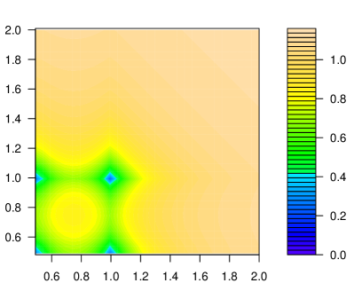
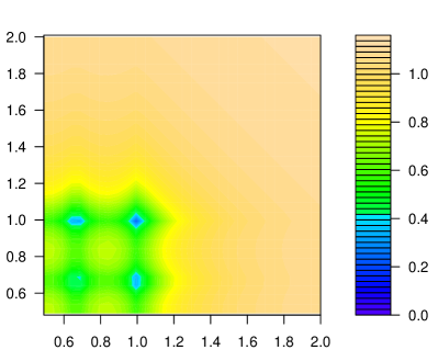
Figure 1: The square root of the MSE of the BLUP for the $N\!\times\!N$-point equidistant design with $N=3$ (left) and $N=4$ (right) and the exponential kernel with $\lambda=2$.

Remark 2.1.

The results of this section can be easily generalized to the case of $d>2$ variables and, moreover, to the model $y(t)=\theta f(t)+\varepsilon(t)$, where $t=(t_{1},\ldots,t_{d})\in\mathcal{T}_{1}\times\ldots\times\mathcal{T}_{d}$, $\mbox{{K}}(t,t^{\prime})=\mathbb{E}[{\varepsilon}(t){\varepsilon}(t^{\prime})]=K_{1}(t_{1},t_{1}^{\prime})\cdots K_{d}(t_{d},t_{d}^{\prime})$ and $f(t)=f_{(1)}(t_{1})\cdots f_{(d)}(t_{d}),$ where $f_{(i)}$ are some functions on $\mathcal{T}_{i}~{};~{}~{}i=1,\ldots,d$.

3 Prediction with derivatives

In this section we consider prediction problems, where the trajectory $y$ in model (1.1) is differentiable (in the mean-square sense) and derivatives of the process (or field) $y$ are available. In Section 3.1 we discuss the discrete case of a once-differentiable process and in Section 3.2 we consider the general case of a $q$ times differentiable (in the mean-square sense) process $y$ satisfying the model (1.1). For the process $y$ to be $q$ times differentiable, the covariance kernel $K$ and vector-function $f$ in (1.1) have to be $q$ times differentiable, which is one of the assumptions in Section 3.2. In Section 3.3 we consider the prediction problem for the location scale model on a two-dimensional product set in the case where the kernel K of the random field ${\varepsilon}$ has the product form (2.12). The results of this section can be easily generalized to the case of $d>2$ variables.

3.1 Discrete case

Consider the model (1.1), where the kernel $K$ and vector-function $f$ are differentiable and one can observe the process $y$ and its derivative at $N$ different points $t_{1},\ldots,t_{N}\in\mathbb{R}$. In this case, the BLUP of $y(t_{0})$ has the form

$$\hat{y}(t_{0})=f^{\top}(t_{0})\hat{\theta}_{\mathrm{BLUE,}{2N}}+K^{\top}_{t_{0},{2N}}\Sigma^{-1}(Y_{2N}-X_{2N}\hat{\theta}_{\mathrm{BLUE,}{2N}}),$$ (3.1)

where $Y_{2N}=(y(t_{1}),\ldots,y(t_{N}),y^{\prime}(t_{1}),\ldots,y^{\prime}(t_{N}))^{\top}\in\mathbb{R}^{2N}$,

$$\Sigma=\left({\Sigma_{00}\atop\Sigma_{10}}{\Sigma^{\top}_{10}\atop\Sigma_{11}}\right)$$

is a block matrix,

$$\Sigma_{00}=\big{(}K(t_{i},t_{j})\big{)}_{i,j=1}^{N},~{}\Sigma_{10}=\Big{(}\frac{\partial}{\partial t_{i}}K(t_{i},t_{j})\Big{)}_{i,j=1}^{N},~{}\Sigma_{11}=\Big{(}\frac{\partial^{2}}{\partial t_{i}\partial t_{j}}K(t_{i},t_{j})\Big{)}_{i,j=1}^{N}$$

are $N\!\times\!N$-matrices,

$$K_{t_{0},{2N}}=\Big{(}K(t_{0},t_{1}),\ldots,K(t_{0},t_{N}),\frac{\partial}{\partial t_{0}}K(t_{0},t_{1}),\ldots,\frac{\partial}{\partial t_{0}}K(t_{0},t_{N})\Big{)}^{\top}$$

is a vector in $\mathbb{R}^{2N}$, $X_{2N}=(f(t_{1}),\ldots,f(t_{N}),f^{\prime}(t_{1}),\ldots,f^{\prime}(t_{N}))^{\top}$ is an $2N\!\times\!m$-matrix and

$$\hat{\theta}_{\mathrm{BLUE,}{2N}}=(X^{\top}_{2N}\Sigma^{-1}_{d}X_{2N})^{-1}X^{\top}_{2N}\Sigma^{-1}_{d}Y_{2N}$$

is the BLUE of $\theta$. The MSE of the BLUP (3.1) is given by

$$\mathrm{MSE}(\hat{y}(t_{0}))=K(t_{0},t_{0})-\left[\begin{matrix}f(t_{0})\\ K_{t_{0},{2N}}\end{matrix}\right]^{\top}\left[\begin{matrix}0&X^{\top}_{2N}\\ X_{2N}&\Sigma_{2N}\end{matrix}\right]^{-1}\left[\begin{matrix}f(t_{0})\\ K_{t_{0},{2N}}\end{matrix}\right].$$

For more general cases of prediction of processes and fields with derivatives observed at a finite number of points, see (Morris et al., 1993; Näther and Šimák, 2003).

3.2 Continuous observations on an interval

Consider the continuous-time model (1.1), where the error process $\epsilon$ has a $q$ times differentiable covariance kernel $K(t,s)$. We also assume that the vector-function $f$ is $q$ times differentiable and therefore the response $y$ is $q$ times differentiable as well.

Suppose we observe realization $y(t)=y^{(0)}(t)$ for $t\in\mbox{{T}}_{0}\subset\mathbb{R}$ and assume that observations of the derivatives $y^{(i)}(t)$ are also available for all $t\in\mbox{{T}}_{i}$, where $\mbox{{T}}_{i}\subset\mathbb{R}$; $i=1,\ldots,q$. The sets $\mbox{{T}}_{i}$ ($i=0,1,\ldots,q$) do not have to be the same; some of these sets (but not all) can even be empty. If at least one of the sets $\mbox{{T}}_{i}$ contains an interval then we speak of a problem with continuous observations.

Consider the problem of prediction of $y^{(p)}(t_{0})$, the $p$-th derivative of $y$ at a point $t_{0}\not\in\mbox{{T}}_{p}$, where $0\leq p\leq q$.

A general linear predictor of the $p$-th derivative $y^{(p)}(t_{0})$ can be defined as

$$\hat{y}_{p,Q}(t_{0})=\int\mathbf{Y}^{\top}(t)\mathbf{Q}(dt)=\sum_{i=0}^{q}\int_{\mbox{{T}}_{i}}y^{(i)}(t)Q_{i}(dt),$$ (3.2)

where $\mathbf{Y}(t)=\left(y(t),y^{(1)}(t),\ldots,y^{(q)}(t)\right)^{\top}$ is a vector with observations of the process and its derivatives, $\mathbf{Q}(dt)=(Q_{0}(dt),\ldots,Q_{q}(dt))^{\top}$ is a vector of length $(q+1)$ and $Q_{0}(dt),\ldots,Q_{q}(dt)$ are signed measures defined on $\mbox{{T}}_{0},\ldots,\mbox{{T}}_{q}$, respectively. The covariance matrix of $\mathbf{Y}(t)$ is

$$\mathbb{K}(t,s)=E[\mathbf{Y}(t)-E\mathbf{Y}(t)][\mathbf{Y}(t)-E\mathbf{Y}(t)]^{\top}=\bigg{(}\frac{\partial^{i+j}K(t,s)}{\partial t^{i}\partial s^{j}}\bigg{)}_{i,j=0}^{q}$$

which is a non-negative definite matrix of size $(q+1)\times(q+1)$.

The estimator $\hat{y}_{p,Q}(t_{0})$ is unbiased if $\mathbb{E}[\hat{y}_{p,Q}(t_{0})]=\mathbb{E}[y^{(p)}(t_{0})]$, which is equivalent to

$$\int\mathbf{F}(t)\mathbf{Q}(dt)=f^{(p)}(t_{0}),$$

where $\mathbf{F}(t)=\left(f(t),f^{(1)}(t),\ldots,f^{(q)}(t)\right)$ is a $m\!\times\!(q+1)$-matrix.

Assumption A^′′.

(1) The best linear unbiased estimator (BLUE) $\hat{\theta}_{\mathrm{BLUE}}=\int\mathbf{G}(dt)\mathbf{Y}(t)$ exists in the model (1.1), where $\mathbf{G}(dt)$ is some signed $m\!\times\!(q+1)$-matrix measure (that is, the $j$-th column of $\mathbf{G}(dt)$ is a signed vector measure defined on ${\mathcal{T}}_{j}$);

(2) There exists a signed vector-measure $\zeta_{p,t_{0}}(dt)$ (of size $q+1$) which satisfies the equation

$$\int\mathbf{K}^{\top}(t,s)\zeta_{p,t_{0}}(dt)=\frac{\partial^{p}K(s,t_{0})}{\partial t_{0}^{p}},\;\;\forall s\in\mbox{{T}}_{i}\,,$$ (3.3)

where $\mathbf{K}(t,s)=\big{(}\frac{\partial^{j}K(t,s)}{\partial s^{j}}\big{)}_{j=0}^{q}$ is a $(q+1)$-dimensional vector.

The problem of existence and construction of the BLUE in the continuous model with derivatives is discussed in (Dette et al., 2019). A general statement establishing the existence and explicit form of the BLUP is as follows. The proof is given in Section 4.

Theorem 3.1.

If Assumption A^′′ holds, then the BLUP measure $\mathbf{Q}_{*}$ exists and is given by

$$\mathbf{Q}_{*}(dt)=\zeta_{p,t_{0}}(dt)+\mathbf{G}^{\top}(dt)c_{p},$$ (3.4)

where the signed measure $\zeta_{p,t_{0}}(dt)$ satisfies (3.3) and

$$c_{p}=f^{(p)}(t_{0})-\int\mathbf{F}(t)\zeta_{p,t_{0}}(dt).$$

The MSE of the BLUP $\hat{y}_{p,Q_{*}}(t_{0})$ is given by

$$\mathrm{MSE}(\hat{y}_{p,Q_{*}}(t_{0}))=\left.\frac{\partial^{2p}K(t,s)}{\partial t^{p}\partial s^{p}}\right|_{{t=t_{0}\atop s=t_{0}}}+c_{p}^{\top}Df^{(p)}(t_{0})-\int\mathbf{K}^{\top}(t,t_{0})\mathbf{Q}_{*}(dt)\,,$$

where

$$D=\int\!\!\int\mathbf{G}(dt)\mathbb{K}(t,s)\mathbf{G}^{\top}(ds)$$

is the covariance matrix of $\hat{\theta}_{\mathrm{BLUE}}=\int\mathbf{G}(dt)\mathbf{Y}(t)$.

Example 3.1.

As a particular case of prediction in the model (1.1), in this example we consider the problem of predicting a value of a process (so that $p=0$) with Matérn $3/2$ covariance kernel $K(t,s)=(1+\lambda|t-s|)e^{-\lambda|t-s|}\,;$ this kernel is once differentiable and is very popular in practice, see e.g. (Rasmussen and Williams, 2006). We assume that the vector-function $f$ in the model (1.1) is 4 times differentiable and that the process $y$ and its derivative $y^{\prime}$ are observed on an interval $[A,B]$ (so that $\mbox{{T}}_{0}=\mbox{{T}}_{1}=[A,B]$ in the general statements). As shown in (Dette et al., 2019), for this kernel the BLUE measure $\mathbf{G}(dt)$ can be expressed in terms of the signed matrix-measure $\zeta(dt)=(\zeta_{0}(dt),\zeta_{1}(dt))$ with

$$\zeta_{0}(dt) = z_{A}\delta_{A}(dt)+z_{B}\delta_{B}(dt)+z(t)dt,$$

$$\zeta_{1}(dt) = z_{1,A}\delta_{A}(dt)+z_{1,B}\delta_{B}(dt),$$

where

$$z_{A} = \frac{1}{4\lambda^{3}}\big{(}f^{(3)}(A)-3\lambda^{2}f^{(1)}(A)+2\lambda^{3}f(A)\big{)},$$

$$z_{1,A} = \frac{1}{4\lambda^{3}}\big{(}-f^{(2)}(A)+2\lambda f^{(1)}(A)-\lambda^{2}f(A)\big{)},$$

$$z_{B} = \frac{1}{4\lambda^{3}}\big{(}-f^{(3)}(B)+3\lambda^{2}f^{(1)}(B)+2\lambda^{3}f(B)\big{)},$$

$$z_{1,B} = \frac{1}{4\lambda^{3}}\big{(}f^{(2)}(B)+2\lambda f^{(1)}(B)+\lambda^{2}f(B)\big{)},$$

$$z(t) = \frac{1}{4\lambda^{3}}\big{(}\lambda^{4}f(t)-2\lambda^{2}f^{(2)}(t)+f^{(4)}(t)\big{)}.$$

Then using (Dette et al., 2019, Sect. 3.4) we obtain $\zeta_{0,t_{0}}(dt)=(\zeta_{0,t_{0},0}(dt),$ $\zeta_{0,t_{0},1}(dt))$ with

$$\zeta_{0,t_{0},0}(dt) = z_{t_{0},A}\delta_{A}(dt)+z_{t_{0},B}\delta_{B}(dt)+z_{t_{0}}(t)dt,$$

$$\zeta_{0,t_{0},1}(dt) = z_{t_{0},1,A}\delta_{A}(dt)+z_{t_{0},1,B}\delta_{B}(dt),$$

where for $t_{0}>B$ we have $z_{t_{0},A}=0$, $z_{t_{0},1,A}=0,$ $z_{t_{0}}(t)=0,$

$$z_{t_{0},B}=(1+\lambda(t_{0}-B))e^{-\lambda(t_{0}-B)},\;\;\;z_{t_{0},1,B}=(t_{0}-B)e^{-\lambda(t_{0}-B)}\,.$$

We also obtain the matrix

$$C=\int_{A}^{B}\zeta_{0}(dt)f^{\top}(t)+\int_{A}^{B}\zeta_{1}(dt){f^{\prime}}^{\top}(t)$$

defined in (Dette et al., 2019, Lem. 2.1) from the condition of unbiasedness. If $D$, the covariance matrix of the BLUE is non-degenerate, then $D=C^{-1}$. In the present case,

$$C = \frac{1}{2}\Big{[}f(A)f^{\top}(A)+f(B)f^{\top}(B)\Big{]}+\frac{1}{2\lambda^{2}}\Big{[}f^{\prime}(A)f^{\prime\top}(A)+f^{\prime}(B)f^{\prime\top}(B)\Big{]}+$$

$$-\frac{1}{4\lambda}\Big{[}f^{\prime}(A)f^{\top}(A)+f(A)f^{\prime\top}(A)+f^{\prime}(B)f^{\top}(B)+f(B)f^{\prime\top}(B)\Big{]}+$$

$$+\frac{1}{4\lambda^{3}}\int_{A}^{B}\Big{[}\lambda^{4}f(t)f^{\top}(t)+2\lambda^{2}f^{\prime}(t)f^{\prime\top}(t)+f^{\prime\prime}(t)f^{\prime\prime\top}(t)\Big{]}dt\,,$$

$$c_{0}=\Big{(}f(t_{0})-[z_{t_{0},B}f(B)+z_{t_{0},1,B}f^{\prime}(B)]\Big{)}.$$

The BLUE-defining measure $\mathbf{G}(dt)$ is expressed through the measures $\zeta(dt)$ and the matrix $C$ by $\mathbf{G}(dt)=C^{-1}\zeta(dt)$. The BLUP measure for process prediction is given by

$$\mathbf{Q}_{*}(dt) = \zeta_{0,t_{0}}(dt)+\mathbf{G}^{\top}(dt)c_{0}$$

$$= \Big{(}\zeta_{0,t_{0},0}(dt)+c_{0}^{\top}C^{-1}\zeta_{0}(dt),\zeta_{0,t_{0},1}(dt)+c_{0}^{\top}C^{-1}\zeta_{1}(dt)\Big{)}^{\top},$$

where

$$c_{0}=f(t_{0})-\int\mathbf{F}(t)\zeta_{0,t_{0}}(dt).$$

For the location scale model with $f(t)=1$, we obtain $C=1+\lambda(B-A)/4$, $c_{0}=(1-z_{t_{0},B})$ and, therefore, a BLUP measure for this model is given by

$$\mathbf{Q}_{*}(dt) = 0.5c_{0}\delta_{A}(dt)/C+(0.5c_{0}/C+z_{t_{0},B})\delta_{B}(dt)+0.25c_{0}\lambda dt/C$$

$$~{}~{}-0.25c_{0}/(C\lambda)\delta_{A}(dt)+(z_{t_{0},1,B}+0.25c_{0}/(C\lambda))\delta_{B}(dt)$$

Therefore, the corresponding BLUP is given

$$\hat{y}_{0,Q_{*}}(t_{0}) = 0.5c_{0}y(A)/C+(0.5c_{0}/C+z_{t_{0},B})y(B)+0.25c_{0}\lambda\int_{A}^{B}y(t)dt/C$$

$$-0.25c_{0}/(C\lambda)y^{\prime}(A)(dt)+(z_{t_{0},1,B}+0.25c_{0}/(C\lambda))y^{\prime}(B).$$

Table 2 gives values of the square root of the MSE of the BLUP in the location scale model at the point $t_{0}=2$ for three families of designs, where $[A,B]=[0,1]$. We observe that observations of derivatives inside the interval do not bring any improvement to the BLUP which can be explained by the fact that the weights of the continuous BLUP at derivatives at points in the interior of the interval $[A,B]$ are $0$.

Table 2: The square root of the MSE of the BLUP at the point $t_{0}=2$ for different designs. (i) the design $\xi_{N,0}$ observing the process at $N$-point equidistant points, (ii) the design $\xi_{N,2}$ observing the process at $N$-point equidistant points and the derivative at two boundary points. (iii) the design $\xi_{N,N}$ observing the process and derivative at $N$-point equidistant points. The model is the location scale model on the interval $[0,1]$ and the covariance kernel of the error process is given by the Matérn 3/2 kernel with $\lambda=2$. For continuous observations the square root of the BLUB is given by $\sqrt{\mathrm{MSE}}=0.9985569896$.

$N$	2	4	8	16
$\xi_{N,0}$	1.059339	1.038152	1.019244	1.009052
$\xi_{N,2}$	0.999276	0.9985675343	0.9985573516	0.9985570068
$\xi_{N,N}$	0.999276	0.9985675343	0.9985573516	0.9985570068

3.3 Location scale model on a product set

Similarly to Section 2.5, we consider the location scale model (2.11) defined on the product set $\mathcal{T}=\mathcal{T}_{1}\times\mathcal{T}_{2}$ (where $\mathcal{T}_{1}$ and $\mathcal{T}_{2}$ are Borel sets in $\mathbb{R}$) with the kernel K of the random field ${\varepsilon}$ having the product form (2.12). The results of this section (as of Section 2.5) can be easily generalized to the case of $d>2$ variables.

Assume that Assumption A^′′ with $q=1$ is satisfied for two one-dimensional models (2.13). For this assumption to hold, the process $\{y(t_{1},t_{2})~{}|~{}(t_{1},t_{2})\in\mathcal{T}\}$ has to be once differentiable with respect to $t_{1}$ and $t_{2}$. Let the measures $G_{0,i}(du)$ and $G_{1,i}(du)$ define the BLUE

$$\int_{\mathcal{T}_{i}}y_{(i)}(u)G_{0,k}(du)+\int_{\mathcal{T}_{i}}y_{(i)}^{(1)}(u)G_{1,i}(du)$$

in the univariate models (2.13); $i=1,2$. In this case, results of (Dette et al., 2019) imply that the BLUE of $\theta$ in the model (2.11) has the form $\hat{\theta}=\int_{\mathcal{T}}{\mathbf{Y}}^{\top}(t)\mbox{ {\bf{G}}}(dt),$ where

$${\mathbf{Y}}^{\top}(t)=\left(y(t),\frac{\partial}{\partial t_{1}}y(t),\frac{\partial}{\partial t_{2}}y(t),\frac{\partial^{2}}{\partial t_{1}\partial t_{2}}y(t)\right)$$

and

$$\mbox{ {\bf{G}}}(dt)=\left(\mbox{{G}}_{00}(dt),\mbox{{G}}_{10}(dt),\mbox{{G}}_{01}(dt),\mbox{{G}}_{11}(dt)\right)^{\top}$$

with $\mbox{{G}}_{ij}(dt)=G_{i,k}(dt_{1})G_{j,k}(dt_{2})$.

Assume we want to predict $y(T)$ at a point $T=(T_{1},T_{2})\notin\mathcal{T}$. The analogue of the equation (2.9) is given by

$$\int_{\mathcal{T}}\mbox{\bf{K}}^{\top}(t,t^{\prime})\mbox{\bf{Z}}_{T}(dt^{\prime})=\mbox{{K}}(t,T),\;\;\forall t\in\mathcal{T},$$ (3.5)

where

$$\mbox{\bf{K}}((t_{1},t_{2}),(s_{1},s_{2}))=\left(\begin{array}[]{l}K_{1}(t_{1},s_{1})K_{2}(t_{2},s_{2})\\ \frac{\partial}{\partial t_{1}}K_{1}(t_{1},s_{1})K_{2}(t_{2},s_{2})\\ K_{1}(t_{1},s_{1})\frac{\partial}{\partial t_{2}}K_{2}(t_{2},s_{2})\\ \frac{\partial}{\partial t_{1}}K_{1}(t_{1},s_{1})\frac{\partial}{\partial t_{2}}K_{2}(t_{2},s_{2})\end{array}\right).$$

Observing the product-form of expressions, we directly obtain that a solution of (3.5) has the form

$$\mbox{\bf{Z}}_{T}(dt_{1},dt_{2})=\left(\begin{array}[]{l}\zeta_{0,T_{1}}(dt_{1})\zeta_{0,T_{2}}(dt_{2})\\ \zeta_{1,T_{1}}(dt_{1})\zeta_{0,T_{2}}(dt_{2})\\ \zeta_{0,T_{1}}(dt_{1})\zeta_{1,T_{2}}(dt_{2})\\ \zeta_{1,T_{1}}(dt_{1})\zeta_{1,T_{2}}(dt_{2})\end{array}\right),$$

where measures $\zeta_{0,T_{i}}(dt)$ and $\zeta_{1,T_{i}}(dt)$ for $i=1,2$ satisfy the equation

$$\int_{\mathcal{T}_{i}}K_{i}(t,s)\zeta_{0,T_{i}}(dt)+\int_{\mathcal{T}_{i}}\frac{\partial}{\partial t}K_{i}(t,s)\zeta_{1,T_{i}}(dt)=K_{i}(s,T_{i}),\;\;\forall s\in{\mathcal{T}_{i}}.~{}$$

Finally, the BLUP at the point $T=(T_{1},T_{2})$ is $\int_{\mathcal{T}}{\mathbf{Y}}^{\top}(t)\mbox{\bf{Q}}_{*}(dt)$, where $\mbox{\bf{Q}}_{*}(dt)=\mbox{\bf{Z}}_{T}(dt)+{c}_{0}\mbox{{\bf{G}}}(dt)$ with $c_{0}=1-\int_{\mathcal{T}}(1,0,0,0)\mbox{\bf{Z}}_{T}(dt).$

The MSE of the BLUP is given by

$$\mathrm{MSE}(\hat{y}_{0,\mbox{\footnotesize\bf{Q}}_{*}}(T))=1+c_{0}D-\int_{\mathcal{T}}\mbox{\bf{K}}^{\top}(t,T)\mbox{\bf{Q}}_{*}(dt),$$

where $D$ is the variance of the BLUE.

Example 3.2.

Consider a location scale model on a square $[0,1]^{2}$ with a product covariance Matérn $3/2$ kernel, that is

$$\mbox{{K}}(t,t^{\prime}) = \mathbb{E}[\varepsilon(t)\varepsilon(t^{\prime})]=K(t_{1},t_{1}^{\prime})K(t_{2},t_{2}^{\prime}),$$

where

$$K(u,u^{\prime})=(1+\lambda|u-u^{\prime}|)e^{-\lambda|u-u^{\prime}|}.$$ (3.8)

Define the measures

$$G_{0}(du)=\frac{1}{4+\lambda}\left[2\delta_{0}(du)+2\delta_{1}(du)+\lambda du\right]$$

and

$$G_{1}(du)=\frac{1}{(4+\lambda)\lambda}\left[\delta_{1}(du)-\delta_{0}(du)\right],\;\;u\in[0,1].$$

In view of (Dette et al., 2019, Sect. 3.4),

$$\int_{0}^{1}y(u)G_{0}(du)+\int_{0}^{1}y^{(1)}(u)G_{1}(du)$$

defines a BLUE in the model $y(u)=\theta+\varepsilon(u)$ with $u\in[0,1]$ and covariance kernel (3.8). Additionally, from (Dette et al., 2019, Sect. 3.4) we have

$$\zeta_{0,T_{i}}(du)=\left\{\begin{array}[]{ll}(1+\lambda|T_{i}|)e^{-\lambda|T_{i}|}\delta_{0}(du),&T_{i}\leq 0,\\ \delta_{T_{i}}(du),&0\leq T_{i}\leq 1,\\ (1+\lambda(T_{i}-1))e^{-\lambda(T_{i}-1)}\delta_{1}(du),&T_{i}\geq 1,\\ \end{array}\right.$$

and

$$\zeta_{1,T_{i}}(du)=\left\{\begin{array}[]{ll}-|T_{i}|e^{-\lambda|T_{i}|}\delta_{0}(du),&T_{i}\leq 0,\\ 0,&0\leq T_{i}\leq 1,\\ (T_{i}-1)e^{-\lambda(T_{i}-1)}\delta_{1}(du),&T_{i}\geq 1.\\ \end{array}\right.$$

Finally, $c_{0}=1-\int_{0}^{1}\!\!\int_{0}^{1}(1,0,0,0)\mbox{\bf{Z}}_{T}(dt)=1-\int_{0}^{1}\!\zeta_{0,T_{1}}(dt_{1})\!\int_{0}^{1}\zeta_{0,T_{2}}(dt_{2})$ and the BLUP measure is given by $\mbox{\bf{Q}}_{*}(dt)=\mbox{\bf{Z}}_{T}(dt)+c_{0}\mbox{{\bf{G}}}(dt);$ that is,

$$\mbox{\bf{Q}}_{*}(dt)=\left(\begin{array}[]{l}\zeta_{0,T_{1}}(dt_{1})\zeta_{0,T_{2}}(dt_{2})+c_{0}G_{0}(dt_{1})G_{0}(dt_{2})\\ \zeta_{1,T_{1}}(dt_{1})\zeta_{0,T_{2}}(dt_{2})+c_{0}G_{1}(dt_{1})G_{0}(dt_{2})\\ \zeta_{0,T_{1}}(dt_{1})\zeta_{1,T_{2}}(dt_{2})+c_{0}G_{0}(dt_{1})G_{1}(dt_{2})\\ \zeta_{1,T_{1}}(dt_{1})\zeta_{1,T_{2}}(dt_{2})+c_{0}G_{1}(dt_{1})G_{1}(dt_{2})\end{array}\right).$$

We now investigate the performance of five discrete designs:

• the design $\xi_{N^{2},0,0,0}$, where we observe process $y$ on an $N\!\times\!N$ grid;

• the design $\xi_{N^{2},4,4,4}$, where we observe process $y$ on an $N\!\times\!N$ grid and additionally derivatives $\frac{\partial y}{\partial t_{1}}$, $\frac{\partial y}{\partial t_{2}}$, $\frac{\partial^{2}y}{\partial t_{1}\partial t_{2}}$ at 4 corners of $[0,1]^{2}$;

• the design $\xi_{N^{2},N^{2},N^{2},0}$, where we observe process $y$ and derivatives $\frac{\partial y}{\partial t_{1}}$, $\frac{\partial y}{\partial t_{2}}$ on an $N\!\times\!N$ grid;

• the design $\xi_{N^{2},N^{2},N^{2},0}$, where we observe process $y$ on an $N\!\times\!N$ grid and derivatives $\frac{\partial y}{\partial t_{1}}$, $\frac{\partial y}{\partial t_{2}}$, $\frac{\partial^{2}y}{\partial t_{1}\partial t_{2}}$ at $4N-4$ equidistant points on the boundary of $[0,1]^{2}$;

• the design $\xi_{N^{2},N^{2},N^{2},N^{2}}$, where we observe process $y$ and derivatives $\frac{\partial y}{\partial t_{1}}$, $\frac{\partial y}{\partial t_{2}}$, $\frac{\partial^{2}y}{\partial t_{1}\partial t_{2}}$ at $N\!\times\!N$ equidistant points on an $N\!\times\!N$ grid.

Table 3: The square root of the MSE of the BLUP at the point $(2,2)$ (upper part) and the point $(0.5,2)$ (lower part) for several designs in the location scale model on the square $[0,1]^{2}$ with Matérn 3/2 product-kernel ($\lambda=2$). The square root of the MSE of the continuous BLUP equals 1.119510 at the point $(2,2)$ and 0.958494 at the point $(0.5,2)$.

$\;\;\;\;\;\;\;\;\;\;\;\;\;N$	2	3	4	8	16
$\xi_{N^{2},0,0,0}$	1.16139	1.15344	1.14972	1.13548	1.12764
$\xi_{N^{2},4,4,4}$	1.121205	1.119682	1.119582	1.119543	1.119528
$\xi_{N^{2},N^{2},N^{2},0}$	1.124401	1.121576	1.120913	1.119893	1.119609
$\xi_{N^{2},4N-4,4N-4,4N-4}$	1.121205	1.119632	1.119535	1.119511	1.119510
$\xi_{N^{2},0,0,0}$	1.03152	1.00413	0.99900	0.97862	0.96862
$\xi_{N^{2},4,4,4}$	0.979953	0.962754	0.963426	0.960604	0.959550
$\xi_{N^{2},N^{2},N^{2},0}$	0.982184	0.958732	0.959663	0.958606	0.958511
$\xi_{N^{2},4N-4,4N-4,4N-4}$	0.979953	0.958566	0.959314	0.958556	0.958500

The results are depicted in Table 3, which shows the square root of the MSE of predictions at the point $(2,2)$ and $(0.5,2)$ for different sample sizes. For any given $N\geq 2$, the MSE for prediction outside the square $[0,1]^{2}$ for the designs $\xi_{N^{2},N^{2},N^{2},N^{2}}$ and $\xi_{N^{2},4N-4,4N-4,4N-4}$ are exactly the same. This is related to the fact that the BLUP weights associated with all derivatives at interior points in $[0,1]^{2}$ of the designs $\xi_{N^{2},N^{2},N^{2},N^{2}}$ are all 0. This means that for optimal prediction of $y(t_{0})$ at a point $t_{0}$ outside the observation region one needs the design guaranteeing the optimal BLUE plus the observations of $y(t)$ and $y^{\prime}(t)$ at points $t$ closest to $t_{0}$. Note that the results of (Dette et al., 2019, Sect. 3.4) imply that the continuous optimal design for the BLUE does not use values of any derivatives of the process (or field for the product-covariance model) in the interior of $\mathcal{T}$.

The observation above is consistent with our other numerical experience which have shown that the BLUP at a point $t_{0}\in(0,1)\times(0,1)$ constructed from the design $\xi_{N^{2},N^{2},N^{2},N^{2}}$ has vanishing weights at all derivatives of interior points of $[0,1]^{2}$ with five exceptions: the center $0$ and the four points which are closest to $t_{0}$ in the $L_{\infty}$ (Manhattan) metric.

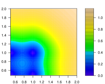
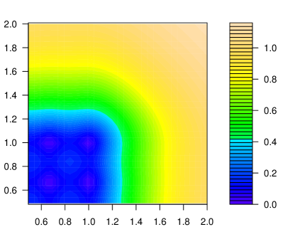
Figure 2: Square root of the MSE of the BLUP for the design $\xi_{N^{2},0,0,0}$ with $N=3$ (left) and $N=4$ (right), and the Matérn 3/2 product-kernel with $\lambda=2$.

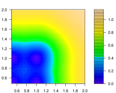
Figure 3: Square root of the MSE of the BLUP for the design $\xi_{N^{2},4N-4,4N-4,4N-4}$ (left) and $\xi_{N^{2},N^{2},N^{2},N^{2}}$ (right) with $N=3$ and the Matérn 3/2 product-kernel with $\lambda=2$.

Figures 2 and 3 compare the MSE for some designs. As Figure 3 illustrates, additionally to Table 3, the MSE for designs $\xi_{N^{2},4N-4,4N-4,4N-4}$ and $\xi_{N^{2},N^{2},N^{2},N^{2}}$ is exactly the same for all points outside $[0,1]^{2}$ and almost the same at all interior points of $[0,1]^{2}$.

4 Proofs

4.1 Proof of Theorem 2.2

To start, we proof the following lemma.

Lemma 4.1.

The mean squared error [relative to the true process value] of any unbiased estimator $\hat{Z}_{Q}=\int_{\mathcal{T}}y(t)Q(dt)$ is given by

$$\mathrm{MSE}(\hat{Z}_{Q})=\mathbb{E}\left(Z-\hat{Z}_{Q}\right)^{2}=$$

$$\!\!\!\int_{\mathcal{S}}\!\int_{\mathcal{S}}\!K(t,s)\nu(dt)\nu(ds)\!-\!2\!\int_{\mathcal{S}}\!\int_{\mathcal{T}}\!K(t,s)\nu(dt)Q(ds)\!+\!\int_{\mathcal{T}}\!\int_{\mathcal{T}}\!Q(dt)K(t,s)Q(ds).$$

Proof. Straightforward calculation gives

$$\!\!\mathrm{MSE}(\hat{Z}_{Q})\!\! = \mathbb{E}\left(Z-\hat{Z}_{Q}\right)^{2}=\mathbb{E}\left(Z-\int_{\mathcal{T}}y(t)Q(dt)\right)^{2}$$

$$= \mathbb{E}\left(\int_{\mathcal{S}}[\theta^{\top}f(t)+\epsilon(t)]\nu(dt)-\int_{\mathcal{T}}[\theta^{\top}f(t)+\epsilon(t)]Q(dt)\right)^{2}$$

$$= \mathbb{E}\left(\int_{\mathcal{S}}\epsilon(t)\nu(dt)-\int_{\mathcal{T}}\epsilon(t)Q(dt)\right)^{2}$$

$$= \!\mathbb{E}\left(\int_{\mathcal{S}}\epsilon(t)\nu(dt)\!-\!\int_{\mathcal{T}}\epsilon(t)Q(dt)\right)\left(\int_{\mathcal{S}}\epsilon(s)\nu(ds)\!-\!\int_{\mathcal{T}}\epsilon(s)Q(ds)\right)$$

$$= \!\int_{\mathcal{S}}\int_{\mathcal{S}}K(t,s)\nu(dt)\nu(ds)\!-\!2\int_{\mathcal{S}}\int_{\mathcal{T}}K(t,s)\nu(dt)Q(ds)$$

$$+\int_{\mathcal{T}}\int_{\mathcal{T}}K(t,s)Q(dt)Q(ds)\,,$$

as required. $\Box$

Let us now prove the main result. We will show that $\mathrm{MSE}(\hat{Z}_{Q})\geq\mathrm{MSE}(\hat{Z}_{Q_{*}})$, where $\hat{Z}_{Q}$ is any linear unbiased estimator of the from (2.7) and $\hat{Z}_{Q_{*}}$ is defined by the measure (2.10). Define $R(dt)=Q(dt)-Q_{*}(dt)$. From the condition of unbiasedness for $Q(dt)$ and $Q_{*}(dt)$, we have $\int_{\mathcal{T}}f(t)R(dt)=0_{m\times 1}$.

We obtain

$$\!\!\!\mathrm{MSE}(\hat{Z}_{Q})\!\!\! = \mathrm{MSE}(\hat{Z}_{Q_{*}+R})$$

$$= \int_{\mathcal{S}}\int_{\mathcal{S}}K(t,s)\nu(dt)\nu(ds)-2\int_{\mathcal{S}}\int_{\mathcal{T}}K(t,s)\nu(dt)[Q_{*}+R](ds)$$

$$+\int_{\mathcal{T}}\int_{\mathcal{T}}[Q_{*}+R](dt){K}(t,s)[Q_{*}+R](ds)$$

$$= \!\!\mathrm{MSE}(Q_{*})\!-\!2\int_{\mathcal{S}}\!\int_{\mathcal{T}}\!K(t,s)\nu(dt)R(ds)\!+\!\int_{\mathcal{T}}\!\int_{\mathcal{T}}\!R(dt){K}(t,s)R(ds)$$

$$+2\int_{\mathcal{T}}\int_{\mathcal{T}}Q_{*}(dt){K}(t,s)R(ds)$$

$$\geq \!\!\mathrm{MSE}(Q_{*})\!-\!2\!\int_{\mathcal{S}}\!\int_{\mathcal{T}}\!K(t,s)\nu(dt)R(ds)\!+\!2\!\int_{\mathcal{T}}\!\int_{\mathcal{T}}\!Q_{*}(dt){K}(t,s)R(ds)$$

$$= \mathrm{MSE}(Q_{*})+2\int_{\mathcal{T}}\Big{[}\int_{\mathcal{T}}Q_{*}(dt){K}(t,s)-\int_{\mathcal{S}}K(t,s)\nu(dt)\Big{]}R(ds)$$

$$= \mathrm{MSE}(Q_{*})+2\int_{\mathcal{T}}c^{\top}Df(s)R(ds)=\mathrm{MSE}(Q_{*})\,,$$

where the inequality follows from nonnegative definiteness of the covariance kernel and the last equality follows from the unbiasedness condition $\int f(t)R(dt)=0$. $\Box$

4.2 Proof of Theorem 3.1

For simplicity, assume $p=0$; the case $p>0$ can be dealt with analogously. First, we derive the following lemma.

Lemma 4.2.

The mean squared error of any unbiased estimator $\hat{y}_{Q}(t_{0})$ of the form (3.2) is given by

$$\!\!\mathrm{MSE}(\hat{y}_{Q}(t_{0}))\!\! = \mathbb{E}\left(y(t_{0})-\hat{y}_{Q}(t_{0})\right)^{2}$$

$$= K(t_{0},t_{0})-2\int_{\mathcal{T}}\mathbf{K}^{\top}(t_{0},s)\mathbf{Q}(ds)+\int_{\mathcal{T}}\int_{\mathcal{T}}\mathbf{Q}^{\top}(dt)\mathbb{K}(t,s)\mathbf{Q}(ds)\,.$$

Proof. Straightforward calculation gives

$$\!\!\!\!\mathrm{MSE}(\hat{y}_{Q}(t_{0}))\!\!\! = \mathbb{E}\left(y(t_{0})-\hat{y}_{Q}(t_{0})\right)^{2}=\mathbb{E}\left(y(t_{0})-\sum_{i=0}^{q}\int_{\mathcal{T}}y^{(i)}(t)Q_{i}(dt)\right)^{2}$$

$$= \mathbb{E}\left(\theta^{\top}f(t_{0})+\epsilon(t_{0})-\sum_{i=0}^{q}\int_{\mathcal{T}}[\theta^{\top}f^{(i)}(t)+\epsilon^{(i)}(t)]Q_{i}(dt)\right)^{2}$$

$$= \mathbb{E}\left(\epsilon(t_{0})-\sum_{i=0}^{q}\int_{\mathcal{T}}\epsilon^{(i)}(t)Q_{i}(dt)\right)^{2}$$

$$= K(t_{0},t_{0})-2\sum_{j=0}^{q}\int_{\mathcal{T}}\frac{\partial^{j}K(t_{0},s)}{\partial s^{j}}Q_{j}(ds)$$

$$+\sum_{i=0}^{q}\sum_{j=0}^{q}\int_{\mathcal{T}}\int_{\mathcal{T}}\frac{\partial^{i+j}K(t,s)}{\partial t^{i}\partial s^{j}}Q_{i}(dt)Q_{j}(ds)\,,$$

as required. $\Box$

Now we will prove the main result. We will show that $\mathrm{MSE}(\hat{y}_{Q}(t_{0}))\geq\mathrm{MSE}(\hat{y}_{Q_{*}}(t_{0}))$, where $\hat{y}_{Q}(t_{0})$ is any linear unbiased estimator of the form (3.2) and $\hat{y}_{Q_{*}}(t_{0})$ is defined by (3.4). Define $\mathbf{R}(dt)=\mathbf{Q}(dt)-\mathbf{Q}_{*}(dt)$. From the condition of unbiasedness for $\mathbf{Q}(dt)$ and $\mathbf{Q}_{*}(dt)$, we have $\int_{\mathcal{T}}\mathbf{F}(t)\mathbf{R}(dt)=0_{m\times 1},$ where $\mathbf{F}(t)=(f(t),f^{(1)}(t),\ldots,f^{(q)}(t))$. Therefore we obtain

$$\!\!\!\mathrm{MSE}(\hat{y}_{Q}(t_{0}))\!\!\! = \mathrm{MSE}(\hat{y}_{Q_{*}+R}(t_{0}))$$

$$= K(t_{0},t_{0})-2\int_{\mathcal{T}}\mathbf{K}^{\top}(t_{0},s)[\mathbf{Q}_{*}+\mathbf{R}](ds)$$

$$+\int_{\mathcal{T}}\int_{\mathcal{T}}[\mathbf{Q}_{*}+\mathbf{R}]^{\top}(dt)\mathbb{K}(t,s)[\mathbf{Q}_{*}+\mathbf{R}](ds)$$

$$= \!\!\mathrm{MSE}(\hat{y}_{Q_{*}}(t_{0}))\!-\!2\!\int_{\mathcal{T}}\!\mathbf{K}^{\top}(t_{0},s)\mathbf{R}(ds)\!+\!\int_{\mathcal{T}}\!\int_{\mathcal{T}}\!\mathbf{R}^{\top}(dt)\mathbb{K}(t,s)\mathbf{R}(ds)$$

$$+2\int_{\mathcal{T}}\int_{\mathcal{T}}\mathbf{Q}_{*}^{\top}(dt)\mathbb{K}(t,s)\mathbf{R}(ds)$$

$$\geq \!\!\mathrm{MSE}(\hat{y}_{Q_{*}}(t_{0}))\!-\!2\!\int_{\mathcal{T}}\!\mathbf{K}^{\top}(t_{0},s)\mathbf{R}(ds)\!+\!2\!\int_{\mathcal{T}}\!\int_{\mathcal{T}}\!\mathbf{Q}_{*}^{\top}(dt)\mathbb{K}(t,s)\mathbf{R}(ds)$$

$$= \mathrm{MSE}(\hat{y}_{Q_{*}}(t_{0}))+2\int_{\mathcal{T}}\Big{[}\int_{\mathcal{T}}\mathbf{Q}_{*}^{\top}(dt)\mathbb{K}(t,s)-\mathbf{K}^{\top}(t_{0},s)\Big{]}\mathbf{R}(ds)$$

$$= \mathrm{MSE}(\hat{y}_{Q_{*}}(t_{0}))+2\int_{\mathcal{T}}c_{p}^{\top}D\mathbf{F}(s)\mathbf{R}(ds)=\mathrm{MSE}(\hat{y}_{Q_{*}}(t_{0}))\,,$$

where the inequality follows from nonnegative definiteness of the covariance kernel and the last equality follows from the unbiasedness condition $\int\mathbf{F}(t)\mathbf{R}(dt)=0$. $\Box$

5 Appendix: more examples of predicting process values

In the appendix, we give further examples of prediction of values of specific random processes $y(t)$, which follows the model (1.1) and observed for all $t\in\mathcal{T}=[A,B]$. In Section 5.1, we illustrate application of Proposition 2.1 and in Section 5.2 we give an example of application of Theorem 3.1. In the example of Section 5.2 we consider the integrated Brownian motion process, which is a once differentiable random process, and we assume that in addition to values of $y(t)$, the values of the derivative of $y(t)$ are also available. As in the main body of the paper, the components of the vector-function $f(t)$ in (1.1) are assumed to be smooth enough (for all formulas to make sense) and linearly independent on $\mathcal{T}$.

5.1 Prediction for Markovian error processes

5.1.1 General Markovian process

Consider the prediction of the random process (1.1) with $\mathcal{T}=[A,B]$ and the Markovian kernel $K(t,s)=u(t)v(s)$ for $t\leq s$, where $u(\cdot)$ and $v(\cdot)$ are twice differentiable positive functions such that $q(t)=u(t)/v(t)$ is monotonically increasing. As shown in (Dette et al., 2019, Sect. 2.6), a solution of the equation $\int_{A}^{B}K(t,s)\zeta(dt)=f(s)$ holding for all $s\in\mathcal{T}$ is the signed vector-measure $\zeta(dt)=z_{A}\delta_{A}(dt)+z_{B}\delta_{B}(dt)+z(t)dt$ with

$$z_{A} = \frac{1}{v^{2}(A)q^{\prime}(A)}\Big{[}\frac{f(A)u^{\prime}(A)}{u(A)}-f^{\prime}(A)\Big{]}\,,\;~{}~{}$$

$$z(t) = -\frac{1}{v(t)}\Big{[}\frac{h^{\prime}(t)}{q^{\prime}(t)}\Big{]}^{\prime}\,,~{}~{}z_{B}=\frac{h^{\prime}(B)}{v(B)q^{\prime}(B)},$$

where $\psi^{\prime}$ denotes a derivative of a function $\psi$, the vector-function $h(\cdot)$ is defined by $h(t)=f(t)/v(t)$.

Then we obtain $\zeta_{t_{0}}(dt)=z_{0A}\delta_{A}(dt)+z_{0B}\delta_{B}(dt)$ with

$$z_{0A}=\frac{1-u^{\prime}(A)}{v^{2}(A)q^{\prime}(A)}v(t_{0}),~{}~{}z_{0B}=\frac{1}{v(B)}v(t_{0}),$$

$$C=\frac{1}{v^{2}(A)q(A)}f(A)f^{\top}(A)+\int_{A}^{B}\frac{[f(t)/v(t)]^{\prime}[f(t)/v(t)]^{\prime\top}}{q^{\prime}(t)}dt$$

and

$$\tilde{c}=C^{-1}c=C^{-1}\left(f(t_{0})-\left[\frac{1-u^{\prime}(A)}{v^{2}(A)q^{\prime}(A)}v(t_{0})f(A)+\frac{1}{v(B)}v(t_{0})f(B)\right]\right).$$

The BLUP measure is given by

$$Q_{*}(dt)=\zeta_{t_{0}}(dt)+c^{\top}G(dt)=\zeta_{t_{0}}(dt)+\tilde{c}^{\top}\zeta(dt)$$

and the MSE of the BLUP is

$$\mathrm{MSE}(\hat{y}_{Q_{*}}(t_{0}))=u(t_{0})v(t_{0})+\tilde{c}^{\top}f(t_{0})-\int_{A}^{B}K(t,t_{0})Q_{*}(dt)\,.$$

5.1.2 Prediction when the error process is Brownian motion

The covariance kernel $K(t,s)=\min(t,s)$ of Brownian motion is a particular case of the Markovian kernel with $u(t)=t$ and $v(s)=1$, $t\leq s$. Further we present the BLUP for few choices of $f(t)$.

For the location-scale model with $f(t)=1$, we obtain $c=0$ and, therefore, the BLUP measure is given by $Q_{*}(dt)=\delta_{B}(dt)$. The BLUP is $\hat{y}_{Q_{*}}(t_{0})=y(B)$ and it has $\mathrm{MSE}(\hat{y}_{Q_{*}}(t_{0}))=t_{0}-B$.

For the model with $f(t)=t$, we obtain $\tilde{c}=B^{-1}(t_{0}-B)$ and, thus, the BLUP measure is given by

$$Q_{*}(dt)=\delta_{B}(dt)+\frac{t_{0}-B}{B}\delta_{B}(dt)=\frac{t_{0}}{B}\delta_{B}(dt).$$

The BLUP is $\hat{y}_{Q_{*}}(t_{0})=\frac{t_{0}}{B}y(B)$ and it has $\mathrm{MSE}(\hat{y}_{Q_{*}}(t_{0}))=\frac{t_{0}}{B}(t_{0}-B)$.

For the model with $f(t)=t^{2}$, we obtain $\tilde{c}=(A^{3}+4/3(B^{3}-A^{3}))^{-1}(t_{0}^{2}-B^{2})$ and, thus, the BLUP measure is given by

$$Q_{*}(dt)=\delta_{B}(dt)+\frac{t_{0}^{2}-B^{2}}{A^{3}+4/3(B^{3}-A^{3})}\Big{(}2B\delta_{B}(dt)-A\delta_{A}(dt)-2dt\Big{)}.$$

The BLUP is

$$\hat{y}_{Q_{*}}(t_{0})=y(B)+\frac{t_{0}^{2}-B^{2}}{A^{3}+4/3(B^{3}-A^{3})}\left(2By(B)-Ay(A)-2\int_{A}^{B}y(t)dt\right)$$

and it has the mean squared error

$$\mathrm{MSE}(\hat{y}_{Q_{*}}(t_{0}))=t_{0}+\tilde{c}\cdot t_{0}^{2}-\int_{A}^{B}t\cdot Q_{*}(dt).$$

5.1.3 Prediction for an OU error process

The covariance kernel $K(t,s)=\exp(-\lambda|t-s|)$ of the OU error process is also a particular case of the Markovian kernel with $u(t)=e^{\lambda t}$ and $v(s)=e^{-\lambda s}$, $t\leq s$.

For the location-scale model $f(t)=1$, we obtain $\tilde{c}=(1+(B-A)\frac{\lambda}{2})^{-1}(1-e^{-\lambda|t_{0}-B|})$ and, therefore, the BLUP measure is given by

$$Q_{*}(dt)=\tilde{c}/2\delta_{A}(dt)+(e^{-\lambda|t_{0}-B|}+\tilde{c}/2)\delta_{B}(dt)+\tilde{c}\lambda/2dt.$$

The BLUP is $\hat{y}_{Q_{*}}(t_{0})=\tilde{c}/2y(A)+(e^{-\lambda|t_{0}-B|}+\tilde{c}/2)y(B)+\tilde{c}\lambda/2\int_{A}^{B}y(t)dt$ and it has $\mathrm{MSE}(\hat{y}_{Q_{*}}(t_{0}))=1+\tilde{c}-\int_{A}^{B}e^{-\lambda|t-t_{0}|}Q_{*}(dt)$.

In Table 4 we give values of the square root of the MSE of the BLUP at the point $t_{0}=2$ for the $N$-point equidistant design in the location scale model on the interval $[0,1]$ and the OU kernel with $\lambda=2$. From this table, we can see that one does not need many points to get almost optimal prediction: indeed, the MSE for designs with $N\geq 4$ is very close to the MSE for the continuous design. Similar results have been observed for other points $t_{0}$ and other Markovian kernels.

Table 4: The square root of the MSE of the BLUP at the point $t_{0}=2$ for the $N$-point equidistant design in the location scale model on the interval $[0,1]$ and the OU kernel with $\lambda=2$; for the continuous design $\sqrt{\mathrm{MSE}}=1.164262$.

$N$	2	4	8	16	32
$\sqrt{\mathrm{MSE}}$	1.18579	1.167157	1.164806	1.164381	1.16429

5.2 Prediction when the error process is integrated Brownian motion

Consider the prediction of the random process (1.1) with $\mathcal{T}=[A,B]$, the 4 times differentiable vector of regression functions $f(t)$ and the kernel of the integrated Brownian motion defined by

$$K(t,s)={\min(t,s)^{2}}(3\max(t,s)-\min(t,s))/{6}.$$

From (Dette et al., 2019, Sect. 3.2) we have that the signed matrix-measure $\zeta(dt)=(\zeta_{0}(dt),\zeta_{1}(dt))$ has components $\zeta_{0}(dt)=z_{A}\delta_{A}(dt)+z_{B}\delta_{B}(dt)+z(t)dt$ and $\zeta_{1}(dt)=z_{1,A}\delta_{A}(dt)+z_{1,B}\delta_{B}(dt)$, where

$$z_{A} = f^{(3)}(A)-\frac{6}{A^{2}}f^{(1)}(A)+\frac{12}{A^{3}}f(A),$$

$$z_{1,A} = -f^{(2)}(A)+\frac{4}{A}f^{(1)}(A)-\frac{6}{A^{2}}f(A),$$

$$z_{B} = -f^{(3)}(B),~{}~{}~{}z_{1,B}=f^{(2)}(B),\;\;z(t)=f^{(4)}(t).$$

Then we obtain $\zeta_{t_{0},0}(dt)=z_{t_{0},A}\delta_{A}(dt)+z_{t_{0},B}\delta_{B}(dt)+z_{t_{0}}(t)dt$ and $\zeta_{t_{0},1}(dt)=z_{t_{0},1,A}\delta_{A}(dt)+z_{t_{0},1,B}\delta_{B}(dt)$ with (for $t_{0}>B$)

$$z_{t_{0},A} = K^{(3)}(A,t_{0})-\frac{6}{A^{2}}K^{(1)}(A,t_{0})+\frac{12}{A^{3}}K(A,t_{0})=0,$$

$$z_{t_{0},1,A} = -K^{(2)}(A,t_{0})+\frac{4}{A}K^{(1)}(A,t_{0})-\frac{6}{A^{2}}K(A,t_{0})=0,$$

$$z_{t_{0},B} = -K^{(3)}(B,t_{0})=1,~{}z_{t_{0},1,B}=K^{(2)}(B,t_{0})=t_{0}-B,$$

and $z_{t_{0}}(t)=K^{(4)}(t,t_{0})=0.$ This implies $\zeta_{t_{0},0}(dt)=\delta_{B}(dt)$ and $\zeta_{t_{0},1}(dt)=(t_{0}-B)\delta_{B}(dt)$. Also we obtain $C=\frac{12}{A^{3}}f(A)f^{\top}(A)-\frac{6}{A^{2}}\Big{(}f^{\prime}(A)f^{\top}(A)+f(A)f^{\prime\top}(A)\Big{)}+\frac{4}{A}f^{\prime}(A)f^{\prime\top}(A)+\int_{A}^{B}f^{\prime\prime}(t)f^{\prime\prime\top}(t)dt$ and $\tilde{c}_{0}\!=\!C^{-1}c_{0}\!=\!C^{-1}\Big{(}f(t_{0})-[f(B)+(t_{0}-B)f^{\prime}(B)]\Big{)}.$

For the location-scale model with $f(t)=1$, we obtain $c=0$ and, therefore, the BLUP measure is given by $\mathbf{Q}_{*}(dt)=(\delta_{B}(dt),(t_{0}-B)\delta_{B}(dt))^{\top}$. The BLUP is $\hat{y}_{\mathbf{Q}_{*}}(t_{0})=y(B)+(t_{0}-B)y^{\prime}(B)$ and it has $\mathrm{MSE}(\hat{y}_{\mathbf{Q}_{*}}(t_{0}))=t_{0}^{3}/3-t_{0}B(t_{0}-B/2).$

Acknowledgments. This work has been supported in part by the Collaborative Research Center “Statistical modelling of nonlinear dynamic processes” (SFB 823, Teilprojekt C2) of the German Research Foundation (DFG). The authors are grateful to Martina Stein, who typed parts of this paper with considerable technical expertise.

References

- Cressie (1993) Cressie, N., 1993. Statistics for Spatial Data. John Wiley & Sons.
- Dette et al. (2019) Dette, H., Pepelyshev, A., Zhigljavsky, A., 2019. The blue in continuous-time regression models with correlated errors. Annals of Statistics 47, 1928–1959.
- Fuentes (2006) Fuentes, M., 2006. Testing for separability of spatial-temporal covariance functions. Journal of Statistical Planning and Inference 136 (2), 447–466.
- Gneiting et al. (2007) Gneiting, T., Genton, M., Guttorp, P., 2007. Geostatistical space-time models, stationarity, separability and full symmetry. In: B. Finkenstadt, L. Held, V. I. (Ed.), Statistical Methods for Spatio-temporal Systems. Chapman and Hall / CRC, Boca Raton, FL, pp. 151–176.
- Leatherman et al. (2017) Leatherman, E. R., Dean, A. M., Santner, T. J., 2017. Designing combined physical and computer experiments to maximize prediction accuracy. Computational Statistics & Data Analysis 113, 346–362.
- Morris et al. (1993) Morris, M. D., Mitchell, T. J., Ylvisaker, D., 1993. Bayesian design and analysis of computer experiments: use of derivatives in surface prediction. Technometrics 35 (3), 243–255.
- Näther and Šimák (2003) Näther, W., Šimák, J., 2003. Effective observation of random processes using derivatives. Metrika 58 (1), 71–84.
- Parzen (1961) Parzen, E., 1961. An approach to time series analysis. The Annals of Mathematical Statistics 32 (4), 951–989.
- Rasmussen and Williams (2006) Rasmussen, C., Williams, C., 2006. Gaussian Processes for Machine Learning. MIT Press.
- Ripley (1991) Ripley, B. D., 1991. Statistical Inference for Spatial Processes. Cambridge University Press.
- Sacks et al. (1989) Sacks, J., Welch, W. J., Mitchell, T. J., Wynn, H. P., 1989. Design and analysis of computer experiments. Statistical Science 4, 409–423.
- Santner et al. (2003) Santner, T. J., Williams, B. J., Notz, W. I., 2003. The Design and Analysis of Computer Experiments. Springer Series in Statistics. New York: Springer-Verlag.
- Stein (1999) Stein, M. L., 1999. Interpolation of Spatial Data: Some Theory for Kriging. Springer Science & Business Media.