A Natural Quadratic Approach to the Generalized Graph Layering Problem

Abstract

We propose a new exact approach to the generalized graph layering problem that is based on a particular quadratic assignment formulation. It expresses, in a natural way, the associated layout restrictions and several possible objectives, such as a minimum total arc length, minimum number of reversed arcs, and minimum width, or the adaptation to a specific drawing area. Our computational experiments show a competitive performance compared to prior exact models.

1 Introduction

Hierarchical graph drawing is an indispensable tool to automate the cleaned-up illustration of e.g. flow diagrams or data dependency representations. Here, the dominant methodological framework studied in research and implemented in software is the one proposed by Sugiyama et al. [9]. It involves four successive and interdependent steps for cycle removal, vertex layering, crossing minimization, and, finally, horizontal coordinate assignment and arc routing.

Classically, the workflow is carried out by solving the feedback arc set problem, i.e., reversing (a minimum number of) arcs, in the first step such that all arcs have a common direction during the others. Then, for the final drawing, original directions are restored. As a result, the height of a graph’s layering is bounded from below by the total height or number of vertices on a longest path after the first step. In particular, a poor aspect ratio of the final drawing may thus be inevitable from the very beginning. Also, the number and placement of dummy vertices, usually introduced if an arc spans a layer to facilitate the other steps and to more accurately account for the width, is strongly affected.

This motivates the recently studied integration of the first two steps [4, 6, 7, 8]. Here, the central idea is to identify (a small number of) suitable arcs to be drawn reverse to the intended hierarchical direction such that this enables a layout that is two-dimensionally compact, possibly meets other common aesthetic criteria such as a minimum total arc length, or even adapts to a drawing area of a certain aspect ratio. Fig. 1 exemplifies the potential effects on aesthetics and readability. Moreover, previous experimental studies in the referenced articles show that significant improvements in terms of the drawing area or aspect ratio are frequent when optimizing the layering with respect to the corresponding objectives.

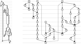
Figure 1: Two layered drawings of the same directed acyclic graph. On the left a classic one, i.e., adhering to its longest path with all arcs pointing downwards, and on the right with a better aspect ratio achieved by reversing only two arcs (drawn dash-dotted).

In this paper, we present a new exact approach to integrate vertex layering, the feedback arc set problem, and width or drawing area optimization. Its most appealing novelty is that it adheres to the quadratic nature of the problem rather than avoiding it. This quadratic nature does not only exist geometrically. Even when optimizing only for one direction (e.g. width), several aspects of a layered drawing depend on conjunctive decisions. For instance, the questions whether an arc is reversed, or whether it causes a dummy vertex on a particular layer, depend on the layer assignments of both of the arc’s end vertices at the same time.

Our approach allows to express such conditions that depend on two simultaneous decisions, and thus all the present generalizations of the classical graph layering problem and their objective functions, in a natural and intuitive way. It is based on a quadratic assignment problem (QAP) formulated and solved as a mixed-integer program (MIP). As our computational results show, it can compete with the currently best known, but less intuitive MIP formulations. This is surprising since the QAP is considered to be among the hardest $\mathcal{NP}$-hard optimization problems. However, the graph layering problem poses a particularly well-suited special case: Our model does not require artificial constructions to model common drawing restrictions and objectives as linear expressions but profits from a sophisticated linearization technique, is compact in the number of constraints, and comparably insensitive to a graph’s density. Ideally, our drawn links to the QAP inspire also new models for related layout styles or heuristic approaches to tackle larger instances or to support interactive user applications.

The paper is organized as follows. In Sect. 2, we give a quick survey of the state of the art generalizations of the classical graph layering problem. The major existing exact approaches to solve these are highlighted in Sect. 3. We then present our quadratic formulation of the most generalized graph layering problem variants in Sect. 4. Finally, we report in Sect. 5 on our computational evaluation, and close with a conclusion in Sect. 6.

2 A Landscape of Graph Layering Problems

A layering $L$ of a directed graph $G=(V,A)$ with vertex set $V$ and arc set $A$ is a mapping $L:V\rightarrow\mathbb{N}^{+}$ that assigns each vertex $v\in V$ a unique layer index $L(v)$. Classically, and presuming that $G$ is acyclic, a layering $L$ is considered feasible if $L(v)-L(u)\geq 1$ holds for all $uv\in A$. In $1993$, the following associated problem was introduced and shown to be polynomial time solvable by Gansner et al. [2]:

Problem 1

Directed Layering Problem (DLP). Let $G=(V,A)$ be a directed acyclic graph. Find a feasible layering $L$ of $G$ minimizing the total arc length

$$\sum_{uv\in A}\big{(}L(v)-L(u)\big{)}.$$

Since, in a final layered drawing of non-acyclic graphs, the presence of reversed arcs is inevitable, and to overcome the limitations mentioned in the introduction (as well for acyclic graphs), a straightforward generalization of DLP discussed by Rüegg et al. [6, 7], is to integrate arc reversals into the layering phase, and thus to consider a layering $L$ feasible if $L(v)\neq L(u)$, i.e., $\lvert L(v)-L(u)\rvert\geq 1$, holds for all $uv\in A$. This gives rise to a second objective besides edge length minimization, namely the minimization of the number of reversed arcs. The trade off between both goals may be addressed by introducing respective weights $\omega_{len}$ and $\omega_{rev}$ into the objective function. The resulting optimization problem is then:

Problem 2

Generalized Layering Problem (GLP). Let $G=(V,A)$ be a directed graph. Find a feasible layering $L$ of $G$ minimizing

$$\omega_{len}\;\Big{(}\sum_{uv\in A}\lvert L(v)-L(u)\rvert\Big{)}\;+\;\omega_{rev}\;\lvert\{uv\in A\mid L(v)<L(u)\}\rvert.$$

As opposed to DLP, GLP is $\mathcal{NP}$-hard, and it remains so even if one of $\omega_{len}$ and $\omega_{rev}$ is zero [6]. Both problems have also been combined with width minimization which is worthwhile, even though the final drawing width is further influenced by the horizontal coordinate assignment and arc routing [7]. In this context, the estimated width $\mathcal{W}$ of a layering is given by the maximum number or maximum total width of original and dummy vertices in any of its layers. With an associated objective function weight $\omega_{wid}$, we have the two according problems:

Problem 3

Minimum Width Directed Layering Problem (DLP-W). Find a layering $L$ of a directed acyclic graph $G=(V,A)$ feasible for DLP that minimizes

$$\omega_{len}\;\Big{(}\sum_{uv\in A}(L(v)-L(u))\Big{)}+\omega_{wid}\;\mathcal{W}.$$

Problem 4

Minimum Width Generalized Layering Problem (GLP-W). Find a layering $L$ of a directed graph $G=(V,A)$ feasible for GLP that minimizes

$$\omega_{len}\;\big{(}\sum_{uv\in A}\lvert L(v)-L(u)\rvert\big{)}\;+\;\omega_{rev}\;\lvert\{uv\in A\mid L(v)<L(u)\}\rvert+\omega_{wid}\;\mathcal{W}.$$

Here, it should be mentioned that DLP-W is equivalent to the precedence-constrained multiprocessor scheduling problem (when ignoring dummy vertices), and thus as well $\mathcal{NP}$-hard [10].

Finally, Rüegg et al. propose to optimize a layering with respect to a target drawing area of width $r_{W}$ and height $r_{H}$ [8]. Informally, a ‘best’ such drawing is considered one that can be maximally scaled (‘zoomed in’) until it exhausts one of the two dimensions (cf. Fig. 1 and 2).

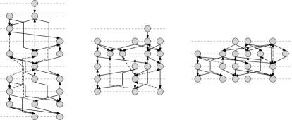
Figure 2: A directed graph drawn based on a layering created by solving GLP-MS with the ratio ${r_{W}:r_{H}}$ set to ${1:2}$ (left), ${1:1}$ (middle), and ${2:1}$ (right). The obtained optimal $\mathcal{W}:\mathcal{H}$ combinations are respectively ${5:10}$, ${6:6}$, and ${8:4}$.

Formally, define $\mathcal{H}\coloneqq\max_{v\in V}L(v)$ to be the height of a layering $L$. This definition is suitable as we may assume w.l.o.g. (and, if necessary, enforce a posteriori for any given and feasible layering) that vertices are assigned to consecutive layers starting from index one. The scaling factor $\mathcal{S}$ to be maximized is then the minimum of the ratios between the targeted and the actually used width and height, respectively, i.e., $\mathcal{S}=\min\{\frac{r_{W}}{\mathcal{W}},\frac{r_{H}}{\mathcal{H}}\}$. Adding once more a corresponding weight $\omega_{scl}$, the problem can be expressed as follows:

Problem 5

Maximum Scale Generalized Layering Problem (GLP-MS). Given a drawing area of (normalized) width $r_{W}$ and (normalized) height $r_{H}$, find a feasible layering $L$ of a directed graph $G=(V,A)$ that minimizes the expression

$$\omega_{len}\;\big{(}\sum_{uv\in A}\lvert L(v)-L(u)\rvert\big{)}+\omega_{rev}\;\lvert\{uv\in A\mid L(v)<L(u)\}\rvert-\omega_{scl}\;\mathcal{S}.$$

A slight variation of GLP-MS as well proposed in [8] will be denoted GLP-MS^∗: Here, instead of minimizing ${-}\omega_{scl}\;\mathcal{S}$, one minimizes $\omega_{scl}\;\bar{\mathcal{S}}$ where $\bar{\mathcal{S}}\coloneqq\frac{1}{\mathcal{S}}$.

3 Evolution of Exact Approaches to Graph Layering

To our best knowledge, all existing exact methods are based on integer programming, and can be coarsely classified based on three different types of variables involved to model the layering of the vertices of a directed graph $G=(V,A)$:

• Assignment-based: Binary variables $x_{v,k}$ taking on value one if $L(v)=k$, and taking on value zero otherwise.

• Ordering-based: This refers to binary variables $y_{k,v}$ taking on value one if $L(v)>k$, and taking on value zero otherwise (see, e.g., the appendix).

• Direct: $L(v)$ is directly modeled as a general integer variable.

Table 1 gives a quick overview of the formulations proposed so far. Some of them are named to ease their reference. Of course, GLP models can solve DLP (by setting $\omega_{rev}=\infty$), width minimization may be turned off (by setting $\omega_{wid}=0$), and models to maximize the scaling factor can be used to minimize the width (by setting $r_{W}=1$ and $r_{H}=\infty$).

Problem	Assignment-based	Ordering-based	Direct
DLP			[2]
DLP-W	WHS [3]
GLP			[7]
GLP-W	EXT [4]	CGL-W [4]
GLP-MS∗		CGL-MS∗ [8]

Table 1: An overview of pre-existing MIP models for the different layering problems.

The direct approach is a perfect fit for the DLP since the resulting problem can be solved in polynomial time by combinatorial algorithms as discussed by Gansner et al. [2]. However, this property (more precisely, the underlying structure) is lost when incorporating width constraints or arc reversals, and the direct method becomes inferior to models with binary variables in practice [7, 4].

The first assignment-based formulation (WHS) was proposed by Healy and Nikolov in [3]. They considered width constraints, but their model may be easily altered to solve DLP-W. Here, the breakthrough to computational tractability for small and medium-sized graphs was to exploit the fixed direction of arcs.

Naturally, this could again not be preserved when it comes to GLP. Rather, modeling whether an arc is reversed or causes a dummy vertex comes then at the cost of additional variables and linearization constraints. Moreover, as Jabrayilov et al. [4] show, the corresponding assignment-based formulation (model EXT) for GLP-W rendered inferior to the first ordering-based one (called CGL-W). Consequently, in [8], Rüegg et al. used the latter as a basis to design a MIP model (that is, to the best of our knowledge, the only one so far) for GLP-MS^∗ and that we thus consistently refer to as CGL-MS^∗.

However, as described in the following, a quadratic assignment-based approach re-enables the possibility to express conditions regarding arc reversals and dummy vertices intuitively, and without artificial linearization constraints.

4 A Natural Quadratic Graph Layering Framework

4.1 A Basic Quadratic Layer Assignment Model (QLA)

Let $G=(V,A)$ be a directed graph, and let $Y$ be an upper bound on the number of layers such that assignment variables $x_{v,k}$ are to be introduced for all $v\in V$ and all $k\in\{1,\dots,Y\}$. Consider as well the variables $p_{u,k,v,\ell}$, for all $uv\in A$ and all $k,\ell\in\{1,\dots,Y\}$, that shall express the product $x_{u,k}\;x_{v,\ell}$. Then, a basic formulation of the layering constraints for any of the GLP problems (DLP as well, but this would permit to be more restrictive) can be expressed as follows:

$$\textstyle\sum\limits_{k=1}^{Y}x_{v,k} =\; 1 \mbox{for all }v\in V$$ (1)

$$\textstyle\sum\limits_{\ell=1}^{Y}p_{u,k,v,\ell} =\; x_{u,k} \mbox{for all }uv\in A,\;k\in\{1,\dots,Y\}$$ (2)

$$\textstyle\sum\limits_{k=1}^{Y}p_{u,k,v,\ell} =\; x_{v,\ell} \mbox{for all }uv\in A,\;\ell\in\{1,\dots,Y\}$$ (3)

$$p_{u,k,v,k} =\; 0 \mbox{for all }uv\in A,\;k\in\{1,\dots,Y\}$$ (4)

$$x_{v,k} \in\; \{0,1\} \mbox{for all }v\in V,\;k\in\{1,\dots,Y\}$$

$$p_{u,k,v,\ell} \in\; [0,1] \mbox{for all }uv\in A,\;k,\ell\in\{1,\dots,Y\}$$

Equations (1) let each vertex be assigned a unique layer. Following the compact linearization approach [5], equations (2) and (3) establish that variable $p_{u,k,v,\ell}=x_{u,k}\cdot x_{v,\ell}$ if the latter two take binary values. As a nice feature of this model, the condition that two adjacent vertices cannot share a common layer can simply be expressed as the variable fixings (4), i.e., the variables may just be omitted in practice. Without accounting for these, the total number of constraints is $2\lvert A\rvert\cdot Y+\lvert V\rvert$, and the total number of variables is $\lvert V\rvert\cdot Y+\lvert A\rvert\cdot(Y-1)^{2}$.

In terms of the latter, the ordering-based CGL models (a compacted reformulation of those in [4] and [8] is displayed in the appendix) are more economical. Even if auxiliary variables for arc reversals or dummy vertices are introduced, their total number is still only $(\lvert V\rvert+\lvert A\rvert)\cdot(Y-1)$. However, the CGL models induce about twice the number of constraints compared to the model above (which is more critical to a MIP solver), and they are more sensitive to a graph’s density.

For any arc $uv\in A$, there is exactly one pair of layers $k$ and $\ell$, $k\neq\ell$, such that $x_{u,k}\cdot x_{v,\ell}=1$. All other products are zero. The length of $uv\in A$ thus equals

$$\textstyle\sum\limits_{\mathclap{k=2}}^{\mathclap{Y}}\textstyle\sum\limits_{\mathclap{\;\;\ell=1}}^{\mathclap{\;k-1}}\;\left((k-\ell)\cdot(x_{u,\ell}\cdot x_{v,k}+x_{u,k}\cdot x_{v,\ell})\right)=\textstyle\sum\limits_{\mathclap{k=2}}^{\mathclap{Y}}\textstyle\sum\limits_{\mathclap{\;\;\ell=1}}^{\mathclap{\;k-1}}\;\left((k-\ell)\cdot(p_{u,\ell,v,k}+p_{u,k,v,\ell})\right).$$

Similarly, the arc $uv\in A$ is reversed if and only if the expression

$$\textstyle\sum\limits_{k=2}^{Y}\left(x_{u,k}\cdot\textstyle\sum\limits_{\ell=1}^{k-1}x_{v,\ell}\right)=\textstyle\sum\limits_{k=2}^{Y}\textstyle\sum\limits_{\ell=1}^{k-1}p_{u,k,v,\ell}$$

evaluates to one. Otherwise, the expression will evaluate to zero.

Finally, an arc $uv\in A$ causes a dummy vertex on a layer $k\in\{2,\dots,Y-1\}$ if and only if $k$ is between the layers $u$ and $v$ are assigned to, i.e., if the expression

$$\textstyle\sum\limits_{\ell=1}^{k-1}\textstyle\sum\limits_{m=k+1}^{Y}(p_{u,\ell,v,m}+p_{u,m,v,\ell})$$

evaluates to one. Again, it will be zero otherwise.

4.2 Quadratic Layer Assignment for GLP-W (QLA-W)

To build model QLA-W from the above basis, it suffices to add a additional continuous variable $\mathcal{W}\in\mathbb{R}_{\geq 0}$ to capture the width together with the $Y$ constraints:

$$\textstyle\sum\limits_{\mathclap{v\in V}}x_{v,k} \leq\; \mathcal{W} \mbox{for all }k\in\{1,Y\}$$

$$\textstyle\sum\limits_{\mathclap{uv\in A}}\;\;\textstyle\sum\limits_{\mathclap{\;\ell=1}}^{\mathclap{\;k-1}}\textstyle\sum\limits_{\mathclap{\;\;\;\;\;\;\;\;\;m=k+1}}^{\;Y}(p_{u,\ell,v,m}+p_{u,m,v,\ell})+\textstyle\sum\limits_{\mathclap{v\in V}}x_{v,k} \leq\; \mathcal{W} \mbox{for all }k\in\{2,\dots,Y-1\}$$

The objective function can be stated as

$$\mbox{minimize }\textstyle\sum\limits_{\mathclap{uv\in A}}\ \big{(}\textstyle\sum\limits_{\mathclap{k=2}}^{\mathclap{Y}}\textstyle\sum\limits_{\mathclap{\;\;\ell=1}}^{\mathclap{\;\;k-1}}\omega_{len}(k-\ell)(p_{u,\ell,v,k}+p_{u,k,v,\ell})+\omega_{rev}\;p_{u,k,v,\ell}\big{)}+\omega_{wid}\;\mathcal{W}.$$

4.3 Quadratic Layer Assignment for GLP-MS^∗ (QLA-MS^∗)

Recalling the definitions from Sect. 2, GLP-MS^∗ asks for the (weighted) minimization of the inverse scaling factor

$$\bar{\mathcal{S}}=\frac{1}{\mathcal{S}}=\frac{1}{\min\{\frac{r_{W}}{\mathcal{W}},\frac{r_{H}}{\mathcal{H}}\}}=\max\big{\{}\frac{\mathcal{W}}{r_{W}},\frac{\mathcal{H}}{r_{H}}\big{\}}.$$

Thus, to obtain model QLA-MS^∗, the basic model is to be extended with an according variable $\bar{\mathcal{S}}\in\mathbb{R}_{\geq 0}$, and with the $Y+\lvert V\rvert$ constraints:

$$\textstyle\sum\limits_{\mathclap{v\in V}}x_{v,k} \leq\; r_{W}\;\bar{\mathcal{S}} \mbox{for all }k\in\{1,Y\}$$

$$\textstyle\sum\limits_{\mathclap{uv\in A}}\;\;\textstyle\sum\limits_{\mathclap{\;\ell=1}}^{\mathclap{\;k-1}}\textstyle\sum\limits_{\mathclap{\;\;\;\;\;\;\;\;\;m=k+1}}^{\;Y}(p_{u,\ell,v,m}+p_{u,m,v,\ell})+\textstyle\sum\limits_{\mathclap{v\in V}}x_{v,k}\!\!\! \leq\; r_{W}\;\bar{\mathcal{S}} \mbox{for all }k\in\{2,\dots,Y-1\}$$

$$\textstyle\sum\limits_{k=1}^{Y}k\;x_{v,k} \leq\; r_{H}\;\bar{\mathcal{S}} \mbox{for all }v\in V$$

Finally, the objective function is

$$\mbox{minimize }\textstyle\sum\limits_{\mathclap{uv\in A}}\ \big{(}\textstyle\sum\limits_{\mathclap{k=2}}^{\mathclap{Y}}\textstyle\sum\limits_{\mathclap{\;\;\ell=1}}^{\mathclap{\;\;k-1}}\omega_{len}(k-\ell)(p_{u,\ell,v,k}+p_{u,k,v,\ell})+\omega_{rev}\;p_{u,k,v,\ell}\big{)}+\omega_{scl}\;\bar{\mathcal{S}}.$$

5 Experimental Evaluation

The aesthetic effects when integrating GLP-MS and GLP-W into the hierarchical framework by Sugiyama et al. were extensively studied already in [4, 6, 7, 8]. Here, we thus confine ourselves to evaluate (i) the computational effects when targeting different aesthetic objectives and aspect ratios, and (ii) the competitiveness of QLA-W and QLA-MS^∗ with respect to CGL-W and CGL-MS^∗.

To accomplish this, we employed the original models CGL-W from [4] and CGL-MS^∗ from [8], except for leaving out constraints that enforce at least one vertex to be placed on the first layer. Also, we employ the same two instance sets as in the mentioned prior studies: The first set ATTar are the AT&T graphs from [1] whereof we extracted all non-tree instances with $20\leq\lvert V\rvert\leq 60$, and $20\leq\lvert A\rvert\leq 168$. Their density $\frac{\lvert A\rvert}{\lvert V\rvert}$ is within $[1,4.72]$ (on average $1.47$). The second set Random consists of $180$ randomly generated and also acyclic and non-tree graphs with $17$ to $60$ vertices, and $30$ to $91$ arcs. These were obtained as follows: First, a respective number of vertices was created. Then, for each vertex, a random number of outgoing arcs (with arbitrary random target) is added such that the total number of arcs is $1.5$ times the number of vertices. Finally, isolated vertices were removed.

During our experiments, all MIPs were solved using Gurobi (release version 8) single-threadedly on a Debian Linux system with an Intel Core i7-3770T CPU ($2.5$ GHz) and $8$ GB RAM, and with a time limit set to half an hour.

5.1 GLP and GLP-W

Here, we consider two experiments. In experiment (1), we set $Y=\lceil 1.6\cdot\sqrt{\lvert V\rvert}\rceil$, $\omega_{len}=1$, $\omega_{rev}=Y\omega_{len}\lvert A\rvert$, and $\omega_{wid}=1$ as in [4]. This can be seen as an almost pure GLP setting, since one saved unit of width has the same (small) effect in the objective function as one saved unit of (total) edge length. Moreover, arcs are reversed only if this is inevitable due to the choice of $Y$ or because they are part of a cycle. In experiment (2), we instead give priority to width minimization by increasing $\omega_{wid}$ to $\omega_{rev}\lvert A\rvert+\lvert A\rvert\cdot Y+1$.

The results are shown in Fig. 3. The most distinctive observation is that the layering problem is considerably harder to solve with both MIPs if emphasis is given to width minimization. In this case, the solution times are higher and several timeouts occur for the larger graphs, while the pure GLP setting can be solved routinely for all instances considered. With respect to experiment (2), the results obtained with QLA-W are slightly better on average than with CGL-W for the ATTar graphs, whereas the opposite is true for the Random graphs, especially due to the increased number of timeouts for the larger ones. Thus, in total, there is no clear superior or inferior model – on average both show a comparable or competitive performance with the MIP solver employed.

Figure 3: The plots depict the solution times in seconds (a cross per graph) for GLP with neglected (1) and emphasized width minimization (2). Crosses at the top (1800$s$) correspond to timeouts, their quantities are given to the left of the respective cross.

5.2 GLP-MS^∗

In this experiment, the parameters are set (almost) as in [8]: $Y=\lvert V\rvert$, $\omega_{len}=1$, $\omega_{rev}=Y\omega_{len}\lvert A\rvert$, and $\omega_{scl}=\omega_{rev}\lvert A\rvert+\lvert A\rvert\cdot Y+1$. Priorities are thus the same as in experiment (2) before, except now emphasizing on a maximum scaling factor instead of the width alone. The ${r_{H}:r_{W}}$ ratios considered are ${1:2}$, ${1:1}$, and ${2:1}$.

Figure 4: The plots depict the solution times in seconds (a cross per graph) for the different ${r_{H}:r_{W}}$ combinations. Crosses at the top (1800$s$) correspond to timeouts, their quantities are given to the left of the respective cross.

As Fig. 4 shows, the results are again diverse under fine-grained inspection, and comparable from a coarse perspective. For both QLA-MS^∗ and CGL-MS^∗ there are instance subsets and ${r_{H}:r_{W}}$ ratios where the use of either one leads to faster solutions and less timeouts.

Also, for both formulations, the ${2:1}$-case, where the height is constrained to be at most twice the width, turns out to be the hardest - which is not surprising as e.g. the ATTar graphs are at least twice as high as wide when drawn with the classic framework [4]. As opposed to that, in the ${1:2}$-case, the condition that the height is restricted to be no more than half of the width is a strong one, as most of the considered graphs cannot be layered very widely. This entails better bounds on the objective function during the MIP solution process.

An interesting question is the relative tractability of GLP-W and (especially the ${2:1}$-case of) the more general GLP-MS^∗, since (in a sense) both aim at a (relatively) small width, but the first with respect to a fixed (but larger) height limit, and the second additionally requiring to find the best ${\mathcal{H}:\mathcal{W}}$-pair under the given aspect ratio constraint. As could be expected, comparing the two results indicates that GLP-W appears to be considerably easier to solve to optimality, at least with the present modeling techniques.

6 Conclusion

In recent years, several extensions of the graph layering problem of increasing generality have been studied, and several algorithmic solution approaches have been proposed. Exact methods are based on integer programming where assignment and ordering variables have dominated the most successful models for the more general variants of the problem.

In this paper, we proposed a new quadratic assignment approach that can be adapted to each of these, allows a natural expression of the associated layout restrictions or aesthetic objectives, and turns out to be computationally competitive. However, as soon as the emphasis is on width minimization or even a particular drawing area is targeted, still neither of the present methods is able to routinely solve arbitrary instances beyond about $50$ vertices. Moreover, as long as the proposed quadratic model is solved based on linearization, its problem size will become a limitation if the number of vertices is considerably increased. Nevertheless, depending on the adjacency structure of the graphs to be layered, this may be possible, and our results show that different settings (aspect ratios, emphasis or neglection of the width, restrictive or non-restrictive heights) have a strong impact on the tractability of the problem – which also means that some can be handled quite well.

Also, the recent generalizations of the layering problem are a clear step towards the requirements of real-world applications – and real-world displays. We hope that our drawn links to the quadratic assignment problem inspire also some novel heuristic solution approaches, or exact models for related graph drawing paradigms.

Appendix 0.A Ordering-based Reference Models

As a reference, we display here slightly more compact reformulations of CGL-W and CGL-MS^∗ compared to their respective original presentations in [4] and [8].

Let $G=(V,A)$ be a directed graph, and let $Y$ be an upper bound on the height of the layering to be chosen a priori. A basic CGL model then involves binary variables $y_{k,v}$, for all ${v\in V}$ and all layer indices $k\in\{1,\dots,Y-1\}$, being equal to $1$ if $k<L(v)$ and being equal to zero otherwise. In particular $L(v)=1$ if and only if $y_{1,v}=0$, $L(v)=Y$ if and only if $y_{k,v}=1$ for all $k\in\{1,\dots,Y-1\}$, and $L(v)=k$ if and only if $y_{k-1,v}-y_{k,v}=1$. The number of basic variables thus amounts to $\lvert V\rvert\cdot(Y-1)$.

Moreover, there are only the following $\lvert V\rvert\cdot(Y-2)$ basic constraints that establish transitivity in the sense that $L(v)>k$ implies $L(v)>k-1$ for each $k\in\{2,\dots,Y-1\}$:

$$y_{k,v}-y_{k-1,v} \leq\; 0 \mbox{for all }v\in V,\;k\in\{2,\dots,Y-1\}$$

However, to model GLP, $\lvert A\rvert$ further auxiliary variables $r_{uv}$ as well as $\lvert A\rvert\cdot Y$ constraints – ensuring that $r_{uv}$ is equal to one if $uv\in A$ is reversed and equal to zero otherwise – are required.

These constraints are:

$$y_{1,u}-r_{uv} \geq\; 0 \mbox{for all }uv\in A$$

$$y_{1,v}+r_{uv} \geq\; 1 \mbox{for all }uv\in A$$

$$y_{k-1,u}-y_{k,v}-r_{uv} \leq\; 0 \mbox{for all }uv\in A,\;k\in\{2,\dots,Y-1\}$$

$$y_{k-1,v}-y_{k,u}+r_{uv} \leq\; 1 \mbox{for all }uv\in A,\;k\in\{2,\dots,Y-1\}$$

$$y_{Y-1,u}-r_{uv} \leq\; 0 \mbox{for all }uv\in A$$

$$y_{Y-1,v}+r_{uv} \leq\; 1 \mbox{for all }uv\in A$$

Moreover, to model dummy vertices (and thus the width), $\lvert A\rvert\cdot(Y-2)$ further variables $d_{uv,k}$ for each arc $uv\in A$ and each layer $k\in\{2,\dots,Y-1\}$ are required. The associated constraints enforcing $d_{uv,k}$ to be one if $uv\in A$ causes a dummy vertex on layer $k$ (otherwise, an optimum solution has $d_{uv,k}=0$ whenever $\omega_{len}>0$) are:

$$y_{k,u}-y_{k-1,v}-d_{uv,k} \leq\; 0 \mbox{for all }uv\in A,\;k\in\{2,\dots,Y-1\}$$

$$y_{k,v}-y_{k-1,u}-d_{uv,k} \leq\; 0 \mbox{for all }uv\in A,\;k\in\{2,\dots,Y-1\}$$

To obtain CGL-W, one further adds a variable $\mathcal{W}$ and the $Y$ constraints:

$$\textstyle\sum\limits_{\mathclap{v\in V}}(1-y_{1,v}) \leq\; \mathcal{W}$$ (5)

$$\textstyle\sum\limits_{\mathclap{v\in V}}y_{Y-1,v} \leq\; \mathcal{W}$$ (6)

$$\textstyle\sum\limits_{\mathclap{v\in V}}(y_{k-1,v}-y_{k,v})+\textstyle\sum\limits_{\mathclap{uv\in A}}d_{uv,k} \leq\; \mathcal{W} \mbox{for all }k\in\{2,\dots,Y-1\}$$ (7)

The total number of constraints is then $(4\lvert A\rvert+\lvert V\rvert+1)\cdot(Y-2)+4\lvert A\rvert+2$. One can now exploit that the length of an arc (i.e., the difference of the layer indices its endpoints are assigned to) is equivalent to the number of dummy vertices it causes plus one. Thus, the objective function for CGL-W can be expressed as:

$$\mbox{minimize }\textstyle\sum\limits_{\mathclap{uv\in A}}\big{(}\omega_{rev}\;r_{uv}+\omega_{len}(1+\!\textstyle\sum\limits_{k=2}^{Y-1}\!d_{uv,k})\big{)}+\omega_{wid}\;\mathcal{W}$$

To rather obtain CGL-MS^∗, it suffices to introduce the variable $\bar{\mathcal{S}}$ instead, replace $\mathcal{W}$ with $r_{W}\;\bar{\mathcal{S}}$ in (5)–(7), and to add the $\lvert V\rvert$ additional constraints:

$$1+\textstyle\sum\limits_{\mathclap{k\in\{1,\dots,Y-1\}}}y_{k,v} \leq\; r_{H}\;\bar{\mathcal{S}} \mbox{for all }v\in V$$

Then, the objective is

$$\mbox{minimize }\textstyle\sum\limits_{\mathclap{uv\in A}}\big{(}\omega_{rev}\;r_{uv}+\omega_{len}(1+\!\textstyle\sum\limits_{k=2}^{Y-1}\!d_{uv,k})\big{)}+\omega_{scl}\;\bar{\mathcal{S}}.$$

and the total number of constraints amounts to $(4\lvert A\rvert+\lvert V\rvert+1)\cdot(Y-2)+4\lvert A\rvert+\lvert V\rvert+2$.

References

- [1] Di Battista, G., Garg, A., Liotta, G., Parise, A., Tamassia, R., Tassinari, E., Vargiu, F., Vismara, L.: Drawing directed acyclic graphs: An experimental study. In: Proceedings of the Symposium on Graph Drawing (GD’96), LNCS, vol. 1190, pp. 76–91. Springer (1997)
- [2] Gansner, E.R., Koutsofios, E., North, S.C., Vo, K.P.: A technique for drawing directed graphs. Software Engineering 19(3), 214–230 (1993)
- [3] Healy, P., Nikolov, N.S.: A branch-and-cut approach to the directed acyclic graph layering problem. In: Goodrich, M.T., Kobourov, S.G. (eds.) Proceedings of the 10th International Symposium on Graph Drawing (GD’02), LNCS, vol. 2528, pp. 98–109. Springer (2002). https://doi.org/10.1007/3-540-36151-0
- [4] Jabrayilov, A., Mallach, S., Mutzel, P., Rüegg, U., von Hanxleden, R.: Compact layered drawings of general directed graphs. In: Hu, Y., Nöllenburg, M. (eds.) Proceedings of the 24th International Symposium on Graph Drawing and Network Visualization (GD’16). pp. 209–221. Springer, Cham (2016)
- [5] Mallach, S.: Compact linearization for binary quadratic problems subject to assignment constraints. 4OR 16(3), 295–309 (Sep 2018). https://doi.org/10.1007/s10288-017-0364-0
- [6] Rüegg, U., Ehlers, T., Spönemann, M., von Hanxleden, R.: A generalization of the directed graph layering problem. Technical Report 1501, Kiel University, Department of Computer Science (Feb 2015), ISSN 2192-6247
- [7] Rüegg, U., Ehlers, T., Spönemann, M., von Hanxleden, R.: A generalization of the directed graph layering problem. In: Hu, Y., Nöllenburg, M. (eds.) Proceedings of the 24th International Symposium on Graph Drawing and Network Visualization (GD’16). pp. 196–208. Springer, Cham (2016)
- [8] Rüegg, U., Ehlers, T., Spönemann, M., von Hanxleden, R.: Generalized layerings for arbitrary and fixed drawing areas. Journal of Graph Algorithms and Applications 21(5), 823–856 (2017). https://doi.org/10.7155/jgaa.00441
- [9] Sugiyama, K., Tagawa, S., Toda, M.: Methods for visual understanding of hierarchical system structures. IEEE Transactions on Systems, Man and Cybernetics 11(2), 109–125 (Feb 1981)
- [10] Ullman, J.D.: NP-complete scheduling problems. Journal of Computer and System Sciences 10(3), 384–393 (1975). https://doi.org/https://doi.org/10.1016/S0022-0000(75)80008-0