Certified answers for ordered quantum discrimination problems

Abstract

We investigate the quantum state discrimination task for sets of linear independent pure states with an intrinsic ordering. This structured discrimination problems allow for a novel scheme that provides a certified level of error, that is, answers that never deviate from the true value more than a specified distance and hence a control of the desired quality of the results. We obtain an efficient semidefinite program and also find a general lower bound valid for any error distance that only requires the knowledge of optimal minimum error scheme. We apply our results to the quantum change point and quantum state anomaly detection cases.

I Introduction

State discrimination plays a fundamental role in quantum information sciences as it determines the capacity of quantum systems to carry information. The task consists in identifying in which of some known set of states a system was prepared by some source. If the possible states are mutually orthogonal this task can be done perfectly. However, if the states are not mutually orthogonal the problem is very nontrivial and it requires optimization with respect to some reasonable criteria.

The most studied discrimination schemes are minimum error (ME) and unambiguous discrimination (UD). In ME after a measurement is performed on the system the experimenter must give an answer about its state. Naturally, some of the answers will be erroneous, and the optimal ME strategy is the one that yields the minimum probability of committing an error Helstrom (1976). In contrast, in UD, no errors are allowed, i.e, the answers of the experimenter must be absolutely certain. This can only be achieved at the expense of permitting inconclusive measurement outcomes. The optimal strategy is the one that minimizes the probability of inconclusive answers. It is known that UD is only possible for sets of linearly independent states Chefles (1998). For mixed states UD is also possible as long as they do not have identical supports Rudolph et al. (2003).

Some extensions of these fundamental schemes have also been considered. Discrimination with maximum confidence Croke et al. (2006) can be applied to states that are not necessarily independent and can be regarded as a generalized UD strategy. Strategies that interpolate between ME and UD have also been studied Bagan et al. (2012). In those a given maximum value for the error probability (or equivalently a maximum value for inconclusive probability) is enforced. Varying this value yields a continuous set of strategies between UD (or maximum confidence) and ME.

Despite being such a fundamental task, analytical solutions for optimal discrimination schemes in the multi-hypothesis case remains a challenge (see Singal et al. (2019) for recent developments). Essentially only the two state Helstrom (1976) and symmetric states cases Ban et al. (1997); Barnett (2001); Krovi et al. (2015) have been solved (see Barnett and Croke (2009); Chefles (2000); Bae and Kwek (2015) for reviews on state discrimination).

In this work we consider a novel multi-hypothesis scheme for sources that prepare states with intrinsic structure. In particular, we consider linear independent states that can be represented as a linear chain (see Fig 1) of $n$ local states. This type of sources includes the interesting cases of change point Sentís et al. (2016, 2017, 2018) and state anomaly detection Skotiniotis et al. (2018) problems. In these structured sources the hypotheses are labelled by some position in the chain, Hence the errors have a natural distance, i.e., we can have have a one-site error, two-site error, etc-., if the outcome of the protocol is an answer that is at distance of one, two, etc., units from the site labelling the true hypothesis. This scheme is interesting not only from the theoretical point of view, but also for practical purposes. In many circumstances not any error can be tolerated, however small deviations from the true hypothesis may have only a limited impact on our decisions. So, it may prove useful to find optimal schemes under the constraint that no outcome can differ from the true hypothesis more than a given threshold distance $\Delta$. Doing so, we have certified answers that will not spoil decisions that we may take upon the outcome of the protocol. We therefore call this scheme certified answer discrimination (CAD). Also if we relax the UA condition and allow some errors, the success probability of guessing the correct hypothesis can increase substantially as we will show. For $\Delta=0$ we recover the UD scheme while for $\Delta=n-1$ we get the ME scheme, thus CAD also provides an interpolation between UD and ME. The interpolating scheme discussed in Bagan et al. (2012) also yield a significant increase in the success probability, but, contrasting the CAD scheme, it may give erroneous answers that are very far from the true value. As it will become clear, CAD is a more natural scheme, closer to the notion of Hamming distances between states (i.e, the sum of positional mismatches Nielsen and Chuang (2011)).

In this paper we give a convenient and efficient semidefinite program (SDP) Vandenberghe and Boyd (1996); Eldar (2003); Watrous (2018) formulation of CAD schemes for linearly independent states. The SDP also enables us to find an analytical lower bound for the probability of success for any allowed error distance $\Delta$. Interestingly, this lower bound only requires to calculate the ME success probability, It provides an approximation on how much the success probability is reduced as we increase the requirements on the quality of the answers of the discrimination protocol.

The paper is organized as follows. In the next Section we present the CAD scheme and its SDP formulation. In Section III we obtain a lower bound for the success probability for any value of $\Delta$. In Section IV we apply our results to the paradigmatic case of the change point and also discuss the state anomaly detection problem. Section IV contains the conclusions of our findings. We also include an appendix with some technical details.

II Certified answer discrimination $\Delta$-schemes

Consider a quantum state multi-hypothesis discrimination problem where the source quantum states have an intrinsic ordering such as a one dimensional chain as depicted in Fig. 1. In this case it is possible to define a natural distance between the states.

Figure 1: Structure of the source states. The position of the blue dot labels the state.

If we are given a state $\left|{\Psi_{k}}\right\rangle$, where $k$ is the position that labels the state, our aim is to find a measurement, generally given by a Positive Operator Value (POVM), that returns the value $k$ with the highest probability. The POVM has to satisfy the additional constraints that no errors beyond some distance $\Delta$ can be committed. For states given by a chain of $n$ states, the POVM contains $n+1$ elements $\{E_{k}\geq 0\}_{k=0}^{n}$, where $E_{0}=\openone-\sum_{k=1}^{n}E_{k}$ is the element corresponding to an inconclusive answer. As in UD this element has to be introduced in order to satisfy the constraints. Naturally as $\Delta$ increases, i.e, more and more type of errors are allowed, we have $\left\langle{\Psi_{k}}\right|E_{0}\left|{\Psi_{k}}\right\rangle\to 0$ for $k=1,2,\ldots,n$.

The optimization problem can be written as the following SDP:

$$\underset{E}{\text{maximize}} \frac{1}{n}\sum_{i=1}^{n}\left\langle{\Psi_{i}}\right|E_{i}\left|{\Psi_{i}}\right\rangle$$ (1)

subject to $$\left\langle{\Psi_{j}}\right|E_{i}\left|{\Psi_{j}}\right\rangle=0\leavevmode\nobreak\ \leavevmode\nobreak\ \forall|i-j|>\Delta$$

$$\sum_{i=1}^{n}E_{i}\leq\mathds{1}$$

$$E_{i}\geq 0\leavevmode\nobreak\ \forall i,$$

where for simplicity we assume that the prior probability is the same for all source states. We will also assume that the source states are linear independent, as naturally happens in the examples considered here (see section IV). Observe that each value $\Delta=0,1,2,\ldots,n-1$ defines a discrimination scheme that we will call a $\Delta$-scheme. Note also that $E_{0}$ is a slack variable that it is taken into account by the inequality $\sum_{i=1}^{n}E_{i}\leq\openone$ in the POVM condition.

For a given value of $\Delta$ we have a probability of success $P_{s}^{\Delta}$, a probability of error $P_{e}^{\Delta}$ and a probability of inconclusive outcome $P_{I}^{\Delta}$, and they satisfy the unitarity condition $P_{s}^{\Delta}+P_{e}^{\Delta}+P_{I}^{\Delta}=1$. The value $\Delta=0$ corresponds to the unambiguous case for which the error probability vanishes, $P_{e}^{\Delta=0}=0$, and the outcome can either perfectly identify the state or be inconclusive, but not erroneous. For $\Delta=n-1$ the are no constraints on the errors and we recover the minimum error scheme, i.e the inconclusive probability vanishes, $P^{\Delta=n-1}_{I}=0$. As we will see later, the minimum error limit can be effectively achieved for much smaller values of $\Delta$.

If the source states are linearly independent, we can transform the SDP (1) into an equivalent and more useful program. From the $n$ linearly independent estates $\{\left|{\Psi_{i}}\right\rangle\}_{i=1}^{n}$ we construct the $R$ matrix,

$$R=\sum_{i=1}^{n}|\Psi_{i}\rangle\langle i|,$$ (2)

where $\left|{i}\right\rangle$ is any orthonormal basis (note that linear independence implies that $R$ is invertible) and consider the new operators $F_{r}^{\Delta}=R^{\dagger}E_{r}^{\Delta}R$. Observe that the diagonal elements of $F_{r}^{\Delta}$ are the expectation values $\left\langle{\Psi_{i}}\right|E_{r}^{\Delta}|\left|{\Psi_{i}}\right\rangle=[F_{r}^{\Delta}]_{i,i}$. Thus, the first constraint in Eq. (1) translates into the condition that all diagonal elements $[F_{r}^{\Delta}]_{i,i}$ vanish except those with $|i-r|\leq\Delta$. Note also that $E_{r}^{\Delta}\geq 0\rightarrow F_{r}^{\Delta}\geq 0$ Bhatia (1996). The off-diagonal terms $[F_{r}^{\Delta}]_{i,j}$ are then also constrained by positivity, and hence we have $[F_{r}^{\Delta}]_{i,j}=0$ for $|r-i|>\Delta$ and $|r-j|>\Delta$. The structure of the matrix $F_{r}^{\Delta}$ is illustrated in Fig. (2).

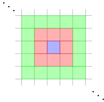
Figure 2: Example of the structure of $F_{r}^{\Delta}=R^{\dagger}E_{r}^{\Delta}R$. The matrices $F_{r}^{\Delta}$ have dimensions $n\times n$ and their non-vanishing elements are depicted as colored boxes. For $\Delta=0$ (no errors), the central blue box is the only non-vanishing element. For $\Delta=1$ (one error) the non-vanishing elements are contained in the red $3\times 3$ block, and in the $5\times 5$ green block for $\Delta=2$, etc. The remaining entries of $F_{r}^{\Delta}$ are all zero.

The second constraint in Eq. (1) can be recast as

$$G-\sum_{r=1}^{n}F_{r}^{\Delta}\geq 0,$$ (3)

by applying the matrix $R^{\dagger}$ on the left and the matrix $R$ on the right. Here $G=R^{\dagger}R$ is the Gram matrix Horn and Johnson (2012) whose elements are

$$G_{i,j}=\langle{\Psi_{i}}|{\Psi_{j}}\rangle.$$ (4)

Thus the SDP (1) is transformed onto

$$\underset{Z}{\text{maximize}} \frac{1}{n}\operatorname{Tr}[ZA]$$ (5)

subject to $$\Phi_{\Delta}[Z]\leq G$$

$$Z\geq 0.$$

The matrix variable $Z$ has a block diagonal structure containing the non-vanishing elements of $F^{\Delta}_{r}$. In Fig. 3 we explicitly depict it for $\Delta=1$. The elements highlighted are the ones that appear in the objective function $\operatorname{Tr}[ZA]$. The constant matrix $A$ depends on the number $n$ of hypothesis and maximum distance $\Delta$ of the allowed errors (we do not add these labels to avoid cluttering too much the notation). Matrix $A$ ”selects” the elements of the matrix variable $Z$ that have to be optimized, i.e., the central elements of the $Z$ blocks. For $\Delta=1$ one has $A=\text{diag}\{1,0,0,1,0,0,1,\ldots,1\}$ and $Z$ and $A$ are $(3n-2)\times(3n-2)$ matrices. The generalization for any $\Delta$ is straightforward. Note that the appearance of the Gram matrix $G$ in the second constraint of (5) showcases that all the discrimination properties of sets of linearly independent states are encapsulated in the Gram matrix.

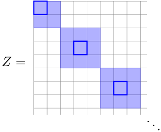
Figure 3: Structure of the matrix variable $Z$ for $\Delta=1$. The blue boxes correspond to the free matrix elements and the blank ones are fixed to be zero. The highlighted boxes are the elements that appear in the objective function $(1/n)\operatorname{Tr}[ZA]$ of Eq. (5).

The linear map $\Phi_{\Delta}$ that incorporates the constraints (3) can be regarded as the action of two linear maps: $\Phi_{\Delta}=\Phi^{2}\circ\Phi^{1}_{\Delta}$. The first map, $\Phi^{1}_{\Delta}$, embeds each block into a $n\times n$ sub-matrix and pads the remaining elements with zeros. The embedding is such that the $k$’th sparse sub-matrix has the central (highlighted) element in the $k$th position of the diagonal, as can be seen in Fig 4. With all the sub-matrices we have an $n^{2}\times n^{2}$ block diagonal matrix. The second map, $\Phi^{2}$, adds the sub-matrices to get a final $n\times n$ matrix, also illustrated in Fig. 4. Notice that this map is independent of $\Delta$.

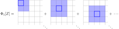
Figure 4: The correspondent map takes the non-zero parts of the variable $Z$ and accommodates it in $n\times n$ matrices with zeros in the remaining places. Observe that matrix sum is defined only for matrices of the same dimensions.

We note that the variable $Z$ from SDP (5) has dimensions $[n(2\Delta+1)-\Delta(\Delta+3)]\times[n(2\Delta+1)-\Delta(\Delta+3)]$ which is significantly lower than $n^{2}\times n^{2}$ of the original SDP (1). The size of the variables is similar only for $\Delta\rightarrow n$. However, as we will see in the quantum change point, the ME limit can be effectively reached for small values of $\Delta$, and then the number of variables remains low for all meaningful values of $\Delta$.

There is no general mathematical method for solving a given SDP analytically, only problems with high degree of symmetry are known to be solvable. In some cases the primal or the dual version of the SDP can suggest an ansatz that may provide the solution (see Sentís et al. (2017) for a nice example). Therefore, any understanding of the form of the solutions of SDPs at hand is of interest. The transformation of the SDP made above proves to be beneficial not only for the numerical advantage but also to obtain insight into how the probability of success behaves in the intermediate regime between unambiguous and minimum error schemes. In particular, it enables us that find useful analytical lower bounds of the probability of success for any $\Delta$ that we discuss in the next section.

III A lower bound for $P_{s}^{\Delta}$

The main idea is to obtain a feasible solution of the SDP (5). Any ansatz matrix $\tilde{Z}$ that satisfies the constraints of an SDP is by construction a lower bound to the optimal solution. The method depends heavily on having previously solved the ME scheme, i.e. we have at our disposal the success probability $P_{s}^{\mathrm{ME}}$, and the corresponding $Z^{\mathrm{ME}}\leavevmode\nobreak\$. Fortunately, in many cases the minimum error scheme can be computed or well approximated with a square root measurement Hausladen and Wootters (1994); Hausladen et al. (1996).

As discussed in previous section the mapping $\Phi_{\Delta}[Z]$ in the SDP (5) can be understood as two step mapping that first transforms the variable $Z$ into a $n^{2}\times n^{2}$ variable that has zeros in appropriate places and a second step that sums all the individual blocks into a $n\times n$ matrix. If we only apply the first map, we get the following SDP:

$$\underset{Z}{\text{maximize}} \frac{1}{n}\operatorname{Tr}[ZA]$$ (6)

subject to $$\Phi_{\Delta}^{1}[Z]\leq Z^{\mathrm{ME}}\leavevmode\nobreak\$$

$$Z\geq 0.$$

Observe that any variable $Z$ that satisfies $\Phi_{\Delta}^{1}[Z]\leq Z^{\mathrm{ME}}\leavevmode\nobreak\$ also satisfies $\Phi_{\Delta}[Z]\leq G$ (just apply the map $\Phi^{2}$, on both sides of the first inequality). Hence, any feasible solution of the SDP (6) is in the feasible set of the SDP (5), but not vice versa, and it provides a lower bound for the probability of success.

For simplicity, let us call $\Phi_{\Delta}^{1}[Z]=Z^{\Delta}$ and $[Z_{r}^{\Delta}]_{i,j}$ the $i,j$ element of its $r$-th sub-matrix $Z_{r}^{\Delta}$. The positivity condition $Z^{\mathrm{ME}}\leavevmode\nobreak\ -Z^{\Delta}\geq 0$ in Eq. (6) implies that any principal minor of $Z^{\mathrm{ME}}\leavevmode\nobreak\ -Z^{\Delta}$ has to be positive Horn and Johnson (2012).

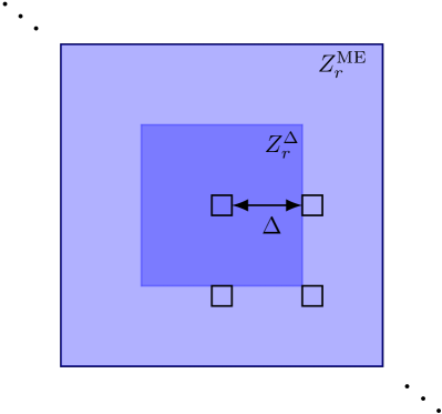
Figure 5: We depict a specific block $r$ of $Z^{\mathrm{ME}}\leavevmode\nobreak\ -Z^{\Delta}$. The light blue block corresponds to $Z^{\mathrm{ME}}_{r}$ and the darker one to $Z^{\Delta}_{r}$. The small black boxes show the elements of the minor of interest to obtain the bound (9).

To get a bound in terms of the known $Z^{\mathrm{ME}}\leavevmode\nobreak\$, the elements of the principal minor have to be outside the central blocks of $Z^{\Delta}$, as depicted in Fig. 5. The choice of this minor is such that it contains only one non-vanishing diagonal element of $Z^{\Delta}$ and three remaining elements are at a $\Delta$ distance and hence take the (known) $Z^{\mathrm{ME}}\leavevmode\nobreak\$ values. We take the minimum distance $\Delta$ as larger distances will give less stringent bounds.

The positivity condition then gives

$$\left([Z^{\mathrm{ME}}\leavevmode\nobreak\ _{i}]_{i,i}-[Z^{\Delta}_{i}]_{i,i}\right)[Z^{\mathrm{ME}}\leavevmode\nobreak\ _{i}]_{i+\Delta+1,i+\Delta+1}\geq$$

$$\left|[Z^{\mathrm{ME}}\leavevmode\nobreak\ _{i}]_{i,i+\Delta+1}\right|^{2}.$$ (7)

Using the fact that the arithmetic mean is bigger than the geometric mean we finally have that

$$\big{(}[Z^{\mathrm{ME}}\leavevmode\nobreak\ _{i}]_{i,i}- [Z^{\Delta}_{i}]_{i,i}\big{)}+[Z^{\mathrm{ME}}\leavevmode\nobreak\ _{i}]_{i+\Delta+1,i+\Delta+1}$$

$$\geq 2\left|[Z^{\mathrm{ME}}\leavevmode\nobreak\ _{i}]_{i,i+\Delta+1}\right|.$$ (8)

As we will be dealing with problems having some symmetry it is convenient to choose this lower minor for the first $\left\lceil n/2\right\rceil$ and the corresponding upper minor for the rest of blocks. For these upper minors we get the same inequality (8) with the change $\Delta\to-\Delta$.

In order to calculate the bound of the success probability only the diagonal elements of $\tilde{Z}$ have to be specified. The best choice is to take them to saturate the inequalities (8), i.e.,

$$[\tilde{Z}_{i}]_{i,i}=\begin{cases}[Z^{\mathrm{ME}}\leavevmode\nobreak\ _{i}]_{i,i}-H_{i}(\Delta)&\mbox{for}\ 1\leq i\leq\left\lceil n/2\right\rceil\\ [Z^{\mathrm{ME}}\leavevmode\nobreak\ _{i}]_{i,i}-H_{i}(-\Delta)&\mbox{for}\ i>\left\lceil n/2\right\rceil\end{cases},$$ (9)

where

$$H_{i}(\Delta)=2\left|[Z^{\mathrm{ME}}\leavevmode\nobreak\ _{i}]_{i,i+\Delta+1}\right|-[Z^{\mathrm{ME}}\leavevmode\nobreak\ _{i}]_{i+\Delta+1,i+\Delta+1}.$$ (10)

Adding all the terms in Eq. (9), the lower bound $\tilde{P}_{s}$ for the success probability reads

$$P_{s}^{\Delta}\geq \tilde{P}_{s}=P_{s}^{\mathrm{ME}}$$

$$- \frac{1}{n}\left[\sum_{i=1}^{\left\lceil n/2\right\rceil}H_{i}(\Delta)+\sum_{i=\left\lceil n/2\right\rceil+1}^{n}H_{i}(-\Delta)\right],$$ (11)

which depends only on $Z^{\mathrm{ME}}\leavevmode\nobreak\$. The bound (11) has two parts, the first is just the success probability of the minimum error case (i.e., the unrestricted case), while the second takes into account how much this value is diminished by the additional constraints imposed by the value $\Delta$. The main virtue of this bound is that given the solution for the minimum error case it provides an expression on how much this probability is lessened by increasing the quality of the answers, i.e., by reducing the maximum allowed distance of the answers to the true state.

IV Applications

In this section we apply our findings to two paradigmatic multi-hypothesis cases. We first discuss the Quantum Change Point (QCP) problem Sentís et al. (2016, 2017, 2018) and then briefly discuss the Quantum State Anomaly Detection (QSAD) problem Skotiniotis et al. (2018).

The QCP problem is depicted in figure (6).

Figure 6: A machine produces a signal state and suddenly it produces another signal. Our task is to determine by measurements the exact moment when this change happens.

A source prepares systems in a default state $|0\rangle$ for some time and suddenly it changes and prepares systems in a mutated state $|\phi\rangle$. Both states are assumed to be known and the change is also assumed to occur at any time with the same probability. The total number of systems is $n$. The goal is to identify the position of the mutation with the highest probability. This is a multi-hypothesis case for which the optimal ME and UD probabilities of success are known Sentís et al. (2016, 2017).

The global states can be written as

$$|\Psi_{k}\rangle=|0\rangle^{\otimes k-1}|\phi\rangle^{\otimes n-k+1}.$$ (12)

The Gram matrix has elements $G_{i,j}=\langle{\Psi_{i}}|{\Psi_{j}}\rangle=c^{|i-j|}$, where $c=\langle{0}|{\phi}\rangle$ and w.l.o.g. can be taken to be in the interval $0\leq c\leq 1$. Note that for $c\neq 0,1$ the off diagonal elements of the $G$ decay exponentially as they depart from the diagonal , which shows that in the QCP the Hamming distance between states is directly related to the overlap between states.

The CAD scheme is particularly pertinent for this problem. It is reasonable to assume that here some deviations of the output guess from the true change point can be tolerated, but not too many in order to avoid jeopardizing the validity of the identification task. In Fig. 7 we show the success probability as a function of $\Delta$ as given by the SDP (5) for $c=0.6$ and $n=25$.

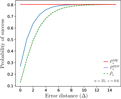
Figure 7: Probability of success versus the allowed error distance $\Delta$ for QCP with $n=25$ and $c=0.6$. The blue solid curve are the exact numerical SDP values (5). The dotted green curve is the analytical lower bound (21). We also show as a reference the red straight line with the value of the minimum error scheme.

We note a remarkable increase in the success probability by just allowing one error deviation of the guess. The value of $P_{s}$ jumps almost a factor of two, from $0.27$ for $\Delta=0$, to $0.50$ for $\Delta=1$. Also the inconclusive probability drops from 0.73 to 0.4, while only 10% of the answers will be erroneous (and just by one position). If these are counted as satisfactory answers, the total success probability goes up to 60%. We have checked that these values of the probabilities essentially remain constant for any $n>25$. We also observe that the probability of success stabilizes to the ME value for $\Delta\gtrsim 8$ (again this threshold value remains the same for larger values of $n$). This just shows that the ME protocol effectively does not yield answers that are at distance greater than eight space units from the true state, as can explicitly be seen in Fig. 8.

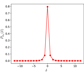
Figure 8: Outcome probability profile of the minimum error scheme of the QCP. The parameter $\delta=\hat{k}-k_{0}$ is the distance of the output guess $\hat{k}$ with respect to the position $k_{0}$ of the true change point. Here $n=25$ , $c=0.6$ and we take the change point to occur at the central position $k_{0}=13$.

We next calculate the bound (11). As discussed in previous section, the bound requires to have the solution $Z^{\mathrm{ME}}\leavevmode\nobreak\$, but, as shown in Sentís et al. (2016), for the QCP can be very well approximated by he square root measurement, i.e. by a projective POVM $\{E_{k}=\left|{m_{k}}\rangle\!\langle{m_{k}}\right|\}_{k=1}^{n}$, with $S\left|{m_{k}}\right\rangle=\left|{\Psi_{k}}\right\rangle$ and $S=\sqrt{G}=\sum_{k}\sqrt{\lambda_{k}}\left|{v_{k}}\rangle\!\langle{v_{k}}\right|$ , where $\lambda_{k}$ and $\left|{v_{k}}\right\rangle$ are the eigenvalues and eigenvectors of $G$, respectively.

The matrix $Z^{\mathrm{ME}}\leavevmode\nobreak\$ in terms of the square root $S$ simply reads

$$Z^{\mathrm{ME}}\leavevmode\nobreak\ =\bigoplus_{k=1}^{n}\left|{s_{k}}\rangle\!\langle{s_{k}}\right|\ \ \mbox{with }\ \ \langle{m_{l}}|{s_{k}}\rangle=S_{l,k},$$ (13)

i.e. $\left|{s_{k}}\right\rangle$ are the column vectors of $S$.

The crucial point to obtain a useful bound is to prove that the elements of $S$ away from the diagonal decay exponentially. From the supplemental material of Sentís et al. (2016) we have

$$S_{k,l}\approx\frac{\sqrt{1-c^{2}}}{\pi}\int_{0}^{\pi}d\theta\frac{(\sin k\theta-c\sin(k-1)\theta)(\sin l\theta-c\sin(l-1)\theta)}{(1-2c\cos\theta+c^{2})^{3/2}}.$$ (14)

After some straightforward algebra Eq. (14) reads

$$S_{k,l} \approx\frac{\sqrt{1-c^{2}}}{4\pi}\int_{-\pi}^{\pi}d\theta\left[\frac{\cos(k-l)\theta-\cos(k+l)\theta}{(1-2c\cos\theta+c^{2})^{1/2}}\right.$$

$$+\left.\chi(k+l,c)\right],$$ (15)

where $\chi(k+l,c)$ contains terms that oscillate rapidly and will be considered later (observe that the second term also oscillates more rapidly than the first). We also note that the explicit terms terms shown in Eq. (15) correspond to the Fourier series of of the function

$$\mu(\theta,c)=\frac{1}{(1-2c\cos\theta+c^{2})^{1/2}},$$ (16)

so we consider

$$\widehat{\mu}(k,c)=\int_{-\pi}^{\pi}\mu(\theta,c)e^{ik\theta}d\theta$$ (17)

for $k\in\mathds{N}$. We prove in Appendix A that $\widehat{\mu}(k,c)$ exhibits an exponential decay in $k$ given by

$$|\widehat{\mu}(r,c)|\leq M_{0}(c)e^{k\log(c)}.$$ (18)

where $M_{0}=\int_{-\pi}^{\pi}\mu(\theta,c)d\theta$. The other terms included in $\chi(k+l,c)$ of Eq. (15))are proportional to $\mu^{3}(r,c)$ and can be tackled in a similar fashion. Including the term proportional to $\cos(k+l)\theta$ and the terms coming from $\chi(k+l,c)$ we get

$$S_{k.l}\leq\frac{\sqrt{1-c^{2}}}{4\pi}\left(M_{0}e^{|k-l|\log(c)}+\sum_{i=-1}^{2}M_{i}e^{(k+l+i)\log(c)}\right).$$ (19)

We can now calculate $Z^{\mathrm{ME}}\leavevmode\nobreak\$ inserting (19) into Eq. (13). We further just take into consideration the (first) dominant term to obtain

$$\left|[Z^{\mathrm{ME}}\leavevmode\nobreak\ _{i}]_{i,i\pm\Delta+1}\right| \leq c\,e^{\Delta\log c}\left|[Z^{\mathrm{ME}}\leavevmode\nobreak\ _{i}]_{i,i}\right|$$

$$\left|[Z^{\mathrm{ME}}\leavevmode\nobreak\ _{i}]_{i\pm\Delta+1,i\pm\Delta+1}\right| \leq c^{2}\,e^{2\Delta\log c}\left|[Z^{\mathrm{ME}}\leavevmode\nobreak\ _{i}]_{i,i}\right|.$$ (20)

Finally from equation (11) we get

$$\tilde{P}_{s}\geq(1-2ce^{\Delta\log c}+c^{2}e^{2\Delta\log c})P_{s}^{\mathrm{ME}},$$ (21)

which shows that the success probability approaches at least exponentially $P_{s}^{\mathrm{ME}}$ for sufficiently large $\Delta$. Note also that in the limit $c\to 0$ we recover the obvious result that $P^{\mathrm{ME}}=P^{\mathrm{UA}}$. We show the bound (21) along with the exact numerical results in figure (7). We observe that indeed the bound approaches the minimum error value for large $\Delta$.

To end this section we study the Quantum State Anomaly Detection (QSAD) problem Dalla Pozza and Pierobon (2015); Skotiniotis et al. (2018) , which will provide some further insight of the features of the our certified answers protocol. QSAD can be regarded as a simplified case of the QCP. The source is assumed to prepare systems in a given default sate $|0\rangle$, however one (and just one) of the local systems was prepared in a different anomalous state $\left|{\phi}\right\rangle$. As in the QCP we assume both states to be known and equal probability for the position of the anomalous state. The task consists in identifying the position of the faulty state with the highest probability when a string of $n$ systems has been prepared. Also here we may consider a protocol that yields guesses not deviating more than $\Delta$ units from the true position of the anomaly.

The set of hypothesis is is given by

$$|\Psi_{k}\rangle=|0\rangle^{\otimes k-1}|\phi\rangle|0\rangle^{\otimes n-k}.$$ (22)

and again we define $c=\langle{\phi}|{0}\rangle$ that w.l.o.g. can be taken to be in the interval $0\leq c\leq 1$. Notice that we have a very simple Gram matrix in this case

$$G_{i,j}=\langle{\psi_{i}}|{\psi_{j}}\rangle=(1-c^{2})\delta_{ij}+c^{2}.$$ (23)

This Gram matrix is circulant Gray (2006) , and hence the square root measurement is optimal Dalla Pozza and Pierobon (2015); Sentís et al. (2016). It is straightforward to find $S=\sqrt{G}$:

$$S_{i,j}=(a-b)\delta_{ij}+b$$ (24)

where

$$a= \frac{\sqrt{1+(n-1)c^{2}}+(n-1)\sqrt{1-c^{2}}}{n}$$

$$b= \frac{\sqrt{1+(n-1)c^{2}}-\sqrt{1-c^{2}}}{n}$$ (25)

Note that the success probability for the minimum error scheme is simply Dalla Pozza and Pierobon (2015)

$$P_{s}^{\mathrm{ME}}=\frac{1}{n}\sum_{i=1}^{n}S_{i,i}^{2}=a^{2}.$$ (26)

The fact that all source states have the same overlap, or equivalently have equal Hamming distance, makes the distance to the true anomaly a less natural parameter in this case and we have different behaviors for $\Delta<\lfloor n/2\rfloor$ and $\Delta\geq\lfloor n/2\rfloor$. It is easy to convince oneself that the symmetry of the problem implies that the condition $\left\langle{\psi_{i}}\right|E_{j}\left|{\psi_{i}}\right\rangle=0$ for $|i-j|\geq\Delta$ for any $\Delta<\lfloor n/2\rfloor$ is in fact equivalent to impose $\Delta=0$ . Whence for $0\leq\Delta<\lfloor n/2\rfloor$ we have a constant probability of success, as can be seen in Fig. 9, and the protocol is equivalent to unambiguous discrimination. It is interesting to calculate the bound (11) in this regime. We have

$$[Z^{\mathrm{ME}}\leavevmode\nobreak\ _{i}]_{ii}=a^{2},\ \ \ [Z^{\mathrm{ME}}\leavevmode\nobreak\ _{i}]_{i,i\pm\Delta+1} =ab$$

$$[Z^{\mathrm{ME}}\leavevmode\nobreak\ _{i}]_{i\pm\Delta+1,i\pm\Delta+1}=b^{2}$$ . (27)

From equation (11) we get

$$\tilde{P}_{s}=(a-b)^{2}=1-c^{2}.$$ (28)

This value is exactly the unambiguous success probability. Notice that for $\Delta=0$, the matrix $A$ in Eq. (5) is $\openone_{n}$ and that by symmetry $Z=z\openone_{n}$, with $z$ a real parameter. Then the SDP reads

maximize $$z$$ (29)

subject to $$z\openone_{n}\leq G$$

$$z\geq 0,$$

which is the SDP for the minimum eigenvalue of $G$. From (23) it is direct to obtain $z=1-c^{2}$, as expected.

For $\Delta\geq\lfloor n/2\rfloor$ we can start having some errors, and the success probability starts to increase from UA to ME as seen in Fig. 9. We also see that the lower bound (11) in this regime departs from the $P_{s}^{\mathrm{UA}}$ value. Now at least one block of $Z^{\mathrm{ME}}\leavevmode\nobreak\$ can be completely covered by $Z^{\Delta}$ which allows for larger contributions to the bound. So $[\tilde{Z}_{j}]_{ii}$ has some elements constrained to be $(a-b)^{2}$ and as $\Delta$ increases new ones equal to the larger value $a^{2}$. Defining $d:=\Delta-\lfloor n/2\rfloor$ and recalling that $P^{\mathrm{ME}}_{s}=a^{2}$ and $P_{s}^{\mathrm{UA}}=(a-b)^{2}$, we obtain from Eq. (11)

$$\tilde{P}_{s}=\begin{cases*}\frac{n-(2d+1)}{n}P_{s}^{\mathrm{UA}}+\frac{2d+1}{n}P_{s}^{\mathrm{ME}}&for \text{$n$ odd}\\ \frac{n-2d}{n}P_{s}^{\mathrm{UA}}+\frac{2d}{n}P_{s}^{\mathrm{ME}}&for \text{$n$ even},\end{cases*}$$ (30)

which exhibits a nice linear behavior interpolating between UA and ME.

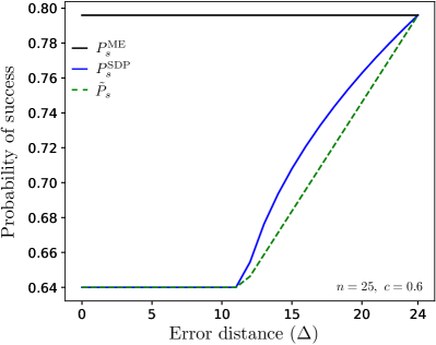
Figure 9: Probability of success against the error distance $\Delta$ for QSAD with $n=25$ and $c=0.6$. The blue solid line shows the numerical results from SDP (5) and the dashed green line the lower bound Eqs. (28) and (30). We also show as a reference a black straight line with the value of the minimum error scheme.

V Conclusions

We have introduced a novel scheme of quantum discrimination for ordered hypothesis of linearly independent states that gives certified answers that do not depart from the true hypothesis more than a given distance $\Delta$. Our scheme may be of practical importance in cases where small deviations from the true hypothesis can be tolerated without compromising the effectiveness of the discrimination task. The scheme allows to tune at will the quality versus the quantity of the answers.

We have shown that all the discrimination properties of a given set of hypotheses are contained in the Gram matrix of the set. We have obtained a compact SDP for the optimal solution that can be solved very efficiently. We have also obtained a lower bound of the success probability for any value of the deviation that only requires the knowledge of the minimum error solution. The bound gives an analytical expression of how much the minimum error success probability is reduced as the maximum distance error $\Delta$ is decreased.

We have applied our findings to the quantum change point problem and the quantum state anomaly detection. For the former, we have shown that allowing a small departure from the true change point increases quite dramatically the success probability. We have computed the lower bound and shown that the increase of the success of probability is exponential in the allowed distance of the errors. For the QSAD we see that up to $n/2$ the protocol is equivalent to unambiguous discrimination. The lower bound for $\Delta\geq n/2$ gives a linear interpolation between UA and ME error protocols.

Our scheme is versatile enough to address other interesting situations. For instance, one might consider non-symmetric errors, i.e the tolerated distance of forward and backward errors may be different. Also one can consider incompatibilities, i.e, given some hypothesis the protocol is required to avoid some specific answers. One important extension of our protocol would be to consider sets of linearly dependent and noisy states. The main difficulty here is how to extend the Gram matrix formalism in these settings. We are currently exploring these scenarios.

Appendix A

In this Appendix we prove that the Fourier coefficients $\widehat{\mu}(k,c)$ of Eq. (17) decay exponentially with $k$ as

$$|\widehat{\mu}(k,c)|\leq M(c)e^{k\log(c)},$$ (31)

where

$$M(c)=\int_{-\pi}^{\pi}\mu(\theta,c)d\theta.$$ (32)

Figure 10: Path of the contour integral of $\mu(z,c)$ in the complex plane.

Proof.

We first extend the function $\mu(\theta,c)$ to the complex plane as

$$\mu(z,c)=\frac{1}{\sqrt{(c-e^{iz})(c-e^{-iz})}}.$$ (33)

If we take the principal branch of the logarithm as a domain of $z\rightarrow\sqrt{z}$ the function $\mu(z,c)$, is analytic in $\mathds{C}/\{-i\log(c),i\log(c)\}$ because it is the composition of several analytic functions. It is a known fact that the Fourier coefficients of analytic functions decay exponentially Katznelson (2004). We next compute

$$\widehat{\mu}(k,c)=\int_{-\pi}^{\pi}\mu(\theta,c)e^{ik\theta}d\theta,$$ (34)

for $k\in\mathds{N}$. Notice that due to the symmetry $\mu(\theta,c)=\mu(-\theta,c)$, only the cosine term of $e^{ik\theta}$ survives. We consider the contour integral in the complex plane shown in Fig. 10. We will call $\gamma^{c}$ the part of the contour that does not lie in the real line. By analyticity of $\mu(z,c)$ in this region we have that,

$$\int_{-\pi}^{\pi}\mu(\theta,c)e^{ik\theta}d\theta+\int_{\gamma^{c}}\mu(z,c)e^{ikz}dz=0.$$ (35)

Notice that $\mu(\theta,c)\geq 0\leavevmode\nobreak\ \forall\leavevmode\nobreak\ \theta\in[-\pi,\pi]$ and $0\leq c\leq 1$, i.e, $\mu(\theta,c)=|\mu(\theta,c)|$. We also see that the contributions of the right and left vertical sections of the path cancel out. Thus, we have

$$\int_{-\pi}^{\pi}|\mu(\theta,c)|d\theta=\int_{-\pi}^{\pi}|\mu(x+i(-\log(c)-\epsilon),c)|dx,$$ (36)

and from Eq. (35) we get

$$\left|\int_{-\pi}^{\pi}\mu(\theta,c)e^{ik\theta}d\theta\right| =\left|\int_{\gamma^{c}}\mu(z,c)e^{ikz}dz\right|$$

$$\leq\int_{\gamma^{c}}\left|\mu(z,c)e^{ikz}\right|dz$$

$$=\int_{\gamma^{c}}\left|\mu(z,c)\right|e^{-ky}dz$$

$$=e^{k(\log(c)+\epsilon)}$$

$$\times\int_{-\pi}^{\pi}|\mu(x+i(-\log(c)-\epsilon),c)|dx$$

$$=M(\epsilon,c)e^{k(\log(c)+\epsilon)},$$

where in going from the second to the third r.h.s expression we use the fact that the the right and left arms contributions of the contour $\gamma^{c}$ cancel out. Note that the constant $M(\epsilon,c)$ does not depend on $k$. Taking the limit $\epsilon\rightarrow 0$ and recalling Eq. (36), we get

$$|\widehat{\mu}(k,c)|\leq e^{k\log(c)}\int_{-\pi}^{\pi}\mu(\theta,c)d\theta,$$ (37)

i.e., $M(c)=\int_{-\pi}^{\pi}\mu(\theta,c)d\theta$. ∎

We can calculate in a completely analogous fashion the Fourier coefficients for other powers of $\mu(\theta,c)$. For instance, the function $\chi(k+l,c)$ in Eq. (15) includes terms proportional to $\mu^{3}(\theta,c)$ and these will also decay exponentially.

All the elements of $S=\sqrt{G}$ of the QCP can thus be expressed as

$$S_{k,l} \leq\frac{\sqrt{1-c^{2}}}{4\pi}\left(M_{0}e^{|k-l|\log(c)}\right.$$

$$+\left.\sum_{i=-1}^{2}M_{i}e^{(k+l+i)\log(c)}\right),$$ (38)

where $M_{i}$ are constants that only depend on $c$ and not on $k$ or $l$.

References

- Helstrom (1976) C. W. Helstrom, Quantum detection and estimation theory (Academic press, 1976).
- Chefles (1998) A. Chefles, Unambiguous discrimination between linearly independent quantum states, Physics Letters A 239, 339 (1998).
- Rudolph et al. (2003) T. Rudolph, R. W. Spekkens, and P. S. Turner, Unambiguous discrimination of mixed states, Physical Review A 68, 010301 (2003).
- Croke et al. (2006) S. Croke, E. Andersson, S. M. Barnett, C. R. Gilson, and J. Jeffers, Maximum confidence quantum measurements, Phys. Rev. Lett. 96, 070401 (2006).
- Bagan et al. (2012) E. Bagan, R. Muñoz-Tapia, G. A. Olivares-Rentería, and J. A. Bergou, Optimal discrimination of quantum states with a fixed rate of inconclusive outcomes, Phys. Rev. A 86, 040303 (2012).
- Singal et al. (2019) T. Singal, E. Kim, and S. Ghosh, Structure of minimum error discrimination for linearly independent states, Phys. Rev. A 99, 052334 (2019).
- Ban et al. (1997) M. Ban, K. Kurokawa, R. Momose, and O. Hirota, Optimum measurements for discrimination among symmetric quantum states and parameter estimation, International Journal of Theoretical Physics 36, 1269 (1997).
- Barnett (2001) S. M. Barnett, Minimum-error discrimination between multiply symmetric states, Phys. Rev. A 64, 030303 (2001).
- Krovi et al. (2015) H. Krovi, S. Guha, Z. Dutton, and M. P. da Silva, Optimal measurements for symmetric quantum states with applications to optical communication, Phys. Rev. A 92, 062333 (2015).
- Barnett and Croke (2009) S. M. Barnett and S. Croke, Quantum state discrimination, Adv. Opt. Photon. 1, 238 (2009).
- Chefles (2000) A. Chefles, Quantum state discrimination, Contemporary Physics 41, 401 (2000), https://doi.org/10.1080/00107510010002599 .
- Bae and Kwek (2015) J. Bae and L.-C. Kwek, Quantum state discrimination and its applications, Journal of Physics A: Mathematical and Theoretical 48, 083001 (2015).
- Sentís et al. (2016) G. Sentís, E. Bagan, J. Calsamiglia, G. Chiribella, and R. Muñoz-Tapia, Quantum change point, Phys. Rev. Lett. 117, 150502 (2016).
- Sentís et al. (2017) G. Sentís, J. Calsamiglia, and R. Muñoz-Tapia, Exact identification of a quantum change point, Phys. Rev. Lett. 119, 140506 (2017).
- Sentís et al. (2018) G. Sentís, E. Martínez-Vargas, and R. Muñoz-Tapia, Online strategies for exactly identifying a quantum change point, Phys. Rev. A 98, 052305 (2018).
- Skotiniotis et al. (2018) M. Skotiniotis, R. Hotz, J. Calsamiglia, and R. Muñoz-Tapia, Identification of malfunctioning quantum devices, arXiv:1808.02729 (2018).
- Nielsen and Chuang (2011) M. A. Nielsen and I. L. Chuang, Quantum Computation and Quantum Information: 10th Anniversary Edition, 10th ed. (Cambridge University Press, New York, NY, USA, 2011).
- Vandenberghe and Boyd (1996) L. Vandenberghe and S. Boyd, Semidefinite programming, SIAM Review 38, 49 (1996).
- Eldar (2003) Y. C. Eldar, A semidefinite programming approach to optimal unambiguous discrimination of quantum states, IEEE Transactions on Information Theory 49, 446 (2003).
- Watrous (2018) J. Watrous, The Theory of Quantum Information (Cambridge University Press, 2018).
- Bhatia (1996) R. Bhatia, Matrix Analysis, Graduate Texts in Mathematics (Springer New York, 1996).
- Horn and Johnson (2012) R. A. Horn and C. R. Johnson, Matrix Analysis, 2nd ed. (Cambridge University Press, New York, NY, USA, 2012).
- Hausladen and Wootters (1994) P. Hausladen and W. K. Wootters, A ‘pretty good’ measurement for distinguishing quantum states, Journal of Modern Optics 41, 2385 (1994).
- Hausladen et al. (1996) P. Hausladen, R. Jozsa, B. Schumacher, M. Westmoreland, and W. K. Wootters, Classical information capacity of a quantum channel, Phys. Rev. A 54, 1869 (1996).
- Dalla Pozza and Pierobon (2015) N. Dalla Pozza and G. Pierobon, Optimality of square-root measurements in quantum state discrimination, Phys. Rev. A 91, 042334 (2015).
- Gray (2006) R. M. Gray, Toeplitz and circulant matrices: A review, Foundations and Trends in Communications and Information Theory 2, 155 (2006).
- Katznelson (2004) Y. Katznelson, An Introduction To Harmonic Analysis, Cambridge Mathematical Library (Cambridge University Press, 2004).