Classification of symmetry-protected topological phases in two-dimensional many-body localized systems

Joey Li Rudolf Peierls Centre for Theoretical Physics, Oxford, 1 Keble Road, OX1 3NP, United Kingdom. Department of Physics, University of Illinois at Urbana-Champaign, Urbana, Illinois 61801, USA.    Amos Chan Rudolf Peierls Centre for Theoretical Physics, Oxford, 1 Keble Road, OX1 3NP, United Kingdom. Physics Department, Princeton University, Princeton, New Jersey 08544, USA.    Thorsten B. Wahl Rudolf Peierls Centre for Theoretical Physics, Oxford, 1 Keble Road, OX1 3NP, United Kingdom. DAMTP, University of Cambridge, Wilberforce Road, Cambridge, CB3 0WA, United Kingdom.
Abstract

We use low-depth quantum circuits, a specific type of tensor networks, to classify two-dimensional symmetry-protected topological many-body localized phases. For (anti-)unitary on-site symmetries we show that the (generalized) third cohomology class of the symmetry group is a topological invariant; however our approach leaves room for the existence of additional topological indices. We argue that our classification applies to quasi-periodic systems in two dimensions and systems with true random disorder within times which scale superexponentially with the inverse interaction strength. Our technique might be adapted to supply arguments suggesting the same classification for two-dimensional symmetry-protected topological ground states with a rigorous proof.

I Introduction

Many-body localization (MBL) Altman and Vosk (2015); Luitz and Lev (2017); Abanin and Papić (2017); Imbrie et al. (2017); Alet and Laflorencie (2017) occurs in isolated strongly disordered systems and is characterized by a lack of thermalization. This phenomenon was first conjectured by Anderson in 1958 as an interacting analogue of Anderson localization Anderson (1958). Theoretical support was lacking until less than fifteen years ago, when perturbation theory analyses Gornyi et al. (2005); Basko et al. (2006), various numerical studies Oganesyan and Huse (2007); Žnidarič et al. (2008); Pal and Huse (2010); Bardarson et al. (2012) and a rigorous proof Imbrie (2016) put the phenomenon in one-dimensional lattice systems on a rigorous footing. In recent years, MBL was also observed in experiments of one-dimensional ultracold atomic gases Schreiber et al. (2015); Lukin et al. (2018) and chains of trapped ions Smith et al. (2016), superconducting qubits Roushan et al. (2017) and NV-centers Choi et al. (2017). Approaches to realizing MBL in solid state systems are currently being pursued Ovadia et al. (2015); Silevitch2017; Wei et al. (2018).

In higher dimensions, truly randomly disordered systems have been suggested to thermalize for arbitrarily large disorder via an avalanche effect due to rare regions Roeck and Imbrie (2017), though assumptions underlying this argument have been contested Potirniche et al. (2019). Furthermore, the avalanche effect is expected to take place on very long time scales Chandran et al. (2016), at least in the limit of small interaction strengths Gopalakrishnan and Huse (2019). This would reconcile the avalanche scenario with very recent ultracold gas experiments, where two-dimensional MBL is observed Choi et al. (2016); Rubio-Abadal et al. (2019). The notion of MBL-like behavior on experimental time scales has since been supported by theoretical studies Thomson and Schiró (2018); Wahl et al. (2019); Kennes (2018); Bertoli et al. (2019); Tomasi et al. (2019); Théveniaut et al. (2019); Kshetrimayum et al. (2019); Geißler and Pupillo (2019), with recent progress in tensor network methods Paeckel et al. (2019); Kloss et al. (2020); Nietner et al. (2020) raising hopes for further insights in the near future. Quasi-periodic potentials in two dimensions lack rare regions and might thus give rise to a stable MBL phase Bordia et al. (2017).

MBL systems are potentially technologically relevant for the storage and manipulation of quantum information Bauer and Nayak (2013); Huse et al. (2013); Chandran et al. (2014a); Potter and Vishwanath (2015): In one dimension, MBL systems with on-site symmetries are able to topologically protect qubits from decoherence caused by local noise at finite energy density Bahri et al. (2015); Goihl et al. (2020). Two dimensional MBL-like systems may display a similar robustness and furthermore be used to manipulate the stored quantum information Parameswaran and Vasseur (2018).

One-dimensional MBL systems with an (anti-)unitary on-site symmetry can be classified into different symmetry-protected topological (SPT) MBL phases Wahl (2018); Chan and Wahl (2020). The different topological classes can be labeled by the elements of the (generalized) second cohomology group of the symmetry group. Note that the symmetry group must be abelian to be compatible with a stable MBL phase Potter and Vasseur (2016). In two dimensions, the expectation is thus that SPT MBL phases are classified by the elements of the third cohomology group, similarly to SPT ground states in two dimensions Chen et al. (2013).

In this work, we use quantum circuits to carry out such a classification in two dimensions. Quantum circuits are a specific type of tensor networks Pérez-García et al. (2007); Verstraete and Cirac (2004); Verstraete et al. (2008); Orùs (2014) and approximate the unitary diagonalizing the MBL Hamiltonian efficiently in one dimension, as indicated by numerical evidence and analytical considerations Pollmann et al. (2016); Wahl et al. (2017). Specifically, the error of the approximation decreases like an inverse polynomial of the computational time (and number of parameters of the approximation). The underlying reason is that all eigenstates of MBL systems fulfill the area law of entanglement Friesdorf et al. (2015) and can thus be efficiently approximated by tensor network states (TNS) Verstraete and Cirac (2006); Pekker and Clark (2017); Devakul et al. (2017); Yu et al. (2017); Pollmann et al. (2016); Wahl et al. (2017). Under the above assumption on the error bound, it is possible to show rigorously that SPT MBL phases are robust to arbitrary symmetry-preserving perturbations and that topologically distinct phases cannot be connected without delocalizing the system Wahl (2018); Chan and Wahl (2020). Furthermore, it follows that all eigenstates of SPT MBL systems have the same topological label as defined for ground states. Here, we use two-dimensional quantum circuits with four layers of unitaries to describe two-dimensional strongly disordered systems. If there is true MBL in two dimensions, our results will apply for all observation times. If instead the avalanche scenario is correct, as we argue below, our classification applies for observation times which are superexponential in the interaction strength for true random disorder. For quasi-periodic disorder, our classification is likely to hold for arbitrarily long observation times in either case.

Concretely, we show that two-dimensional MBL phases invariant under a symmetry can be labeled by the elements of the third cohomology group of the symmetry group. However, we cannot rule out the existence of additional topological indices with our approach. Furthermore, we show that the topological labels we find are robust to symmetry-preserving perturbations and cannot be connected without destroying MBL-like behavior. Again, it follows that all eigenstates must have the same topological label. We anticipate that our two-dimensional quantum circuit approach might be adapted to carry out a rigorous classification of two-dimensional SPT ground states, which is currently an outstanding problem Cirac et al. (2019). Note that our classification does not apply to topologically ordered MBL systems Parameswaran and Vasseur (2018), as their Hamiltonians cannot be diagonalized by short-depth quantum circuits Wahl and Béri (2020).

This article is structured as follows: In Section II we give a more formal introduction to the theoretical description of MBL systems in one and two dimensions, their SPT phases and tensor networks. Section III contains a non-technical summary of our results with the technical part provided in Sections IV (unitary on-site symmetries) and V (anti-unitary on-site symmetries). Section VI discusses the robustness of the obtained topological phases to symmetry-preserving perturbations and demonstrates that the only way of connecting topologically distinct MBL phases is by either breaking the symmetry or making the perturbation strong enough to destroy MBL-like behavior. In Section VII, we summarize our results and present directions for future work. In the Appendix, we provide technical details on the interpretation of the elements of the second and third cohomology group in terms of projective and gerbal representations, respectively.

II Symmetry-protected topological many-body localized phases and tensor networks

Here we briefly review the central ideas about many-body localization and symmetry-protected topological phases and introduce tensor network language. Readers already familiar with these topics may easily skip this Section. For a similar but slightly more complete review of SPT and MBL, see Section II of Ref. Chan and Wahl, 2020.

II.1 Many-body localization in one dimension

Here, we briefly review MBL in one dimension before commenting on the two-dimensional case. The canonical model of strongly disordered Hamiltonians that exhibits MBL in one dimension is the random field Heisenberg model Oganesyan and Huse (2007); Pal and Huse (2010),

$$H=J\sum_{i=1}^{N-1}\mathbf{S}_{i}\cdot\mathbf{S}_{i+1}+\sum_{i=1}^{N}h_{i}S^{z}_{i},$$ (1)

where $J>0$, and $h_{i}$ is sampled from a uniform distribution $[-W,W]$. (1) displays a transition from the ergodic phase to the MBL phase as a function of the disorder strength controlled by $W$. Numerical studies indicate a phase transition at around $W_{c}\approx 3.5J$ Pal and Huse (2010); Luitz et al. (2015).

Below but close to the phase transition (1) exhibits a mobility edgeLuitz et al. (2015): Eigenstates in an energy window in the middle of the spectrum are volume law entangled, while eigenstates outside of this window are area law entangled. For SPT phases we are interested in the fully many-body localized (FMBL) phase ($W\gtrsim 3.5J$ for (1)), where all eigenstates are area law entangled. The FMBL phase is described by a complete set of local integrals of motion (LIOMs)Serbyn et al. (2013); Huse et al. (2014) $\tau_{i}^{z}$. This remains true after adding small but non-zero arbitrary local perturbations, even in the thermodynamic limit. Any resonances of distant spins with similar energies are captured by those LIOMs (which would in that case be particularly wide). We do not consider the case of resonances spreading across the whole system in the thermodynamic limit. In that case, there are volume law entangled eigenstates, which would correspond to a disorder strength below the phase transition point as defined above (where a mobility edge is present and the LIOM picture does not apply). Here we refer to the actual MBL-to-thermal phase transition point in the thermodynamic limit, which might be significantly higher than the value quoted above due to finite size effects Doggen et al. (2018); Abanin et al. (2019). (However, the effect of rare regions on the transition point in the thermodynamic limit has also been questioned in one dimension Goihl et al. (2019). Moreover, MBL systems coupled to thermal baths have been argued to delocalize only if the latter take a finite fraction of the overall system size Sparaciari et al. (2019).)

LIOMs are local operators which commute with the Hamiltonian and with each other, and therefore form an emergent notion of integrability,

$\displaystyle[H,\tau_{i}^{z}]=[\tau_{i}^{z},\tau_{j}^{z}]=0$ (2)

for all $i,j=1,2,\ldots,N$. Hence, all eigenstates $|\psi_{l_{1}l_{2}\ldots l_{N}}\rangle$ of the Hamiltonian can be uniquely labeled by the expectation values (say $l_{i}=\pm 1$, also known as l-bits) of the corresponding $\tau_{i}^{z}$ operators. (Here we consider the case of spin-$1/2$ Hamiltonians, though the notion of LIOMs can be straightforwardly generalized to higher spin systems.) According to Eq. (2), the LIOMs and the Hamiltonian can all be simultaneously diagonalized by a unitary $U$, that is,

$\displaystyle H$ $\displaystyle=UEU^{\dagger},$ (3)
$\displaystyle\tau_{i}^{z}$ $\displaystyle=U\sigma_{i}^{z}U^{\dagger}.$ (4)

Any Hamiltonian could be used to construct a commuting set of integrals of motion this way. The special feature of FMBL systems is that the unitary $U$ can be chosen such that the $\tau_{i}^{z}$ are local, i.e., they have exponentially decaying support from site $i$. The corresponding decay length is known as the localization length $\xi_{i}$. The corresponding unitary $U$ has been argued to be efficiently approximable by a short-depth quantum circuit with long gates Wahl et al. (2017); Wahl (2018). The exact distribution of localization lengths $\xi_{i}$ for a given system size $N$ depends on the disorder realization. The probability of finding localization length within a range $[\xi,\xi+\Delta\xi]$ decays sharply with $\xi$ Kulshreshtha et al. (2018). For a system to be considered as FMBL, we have to assume that the probability that the largest localization length $\xi_{\mathrm{max}}$ is of order $\mathcal{O}(N)$ goes to zero in the limit $N\rightarrow\infty$ (otherwise, the system would be delocalized). Hence, we assume $\xi_{\mathrm{max}}\leq cN^{\mu}$ for a given disorder realization and model Hamiltonian (such as Eq. (1)) with constants $c>0$ and $\mu\in[0,1)$.

II.2 Many-body localization in higher dimensions

It is believed that in higher dimensions for true random disorder, regions with anomalously small disorder will eventually thermalize the entire system Roeck and Imbrie (2017); Gopalakrishnan and Huse (2019), although this picture has to be taken with care Potirniche et al. (2019). Regions with anomalously small disorder contain small thermal inclusions, i.e., local expectation values of all eigenstates look thermal in those regions. This phenomenon also arises in one dimension, and, in the above framework, implies a set of particularly wide LIOMs (with large localization lengths $\xi_{i}$). While in one dimension such a set of wide LIOMs can be stable, it is believed that in higher dimensions sufficiently large thermal regions cannot remain isolated, as they would gradually thermalize surrounding spins and thus grow via an avalanche effect until the whole system becomes thermal Doggen et al. (2020). For concreteness, let us consider a $d$-dimensional cubic lattice with $N^{d}$ spins described by the general Hamiltonian of Ref. Gopalakrishnan and Huse, 2019

$\displaystyle H=\sum_{i}h_{i}O_{i}+J\sum_{i,j}\phi_{ij}P_{ij}.$ (5)

$h_{i}$ are random fields chosen from a uniform distribution centered around zero. $\phi_{ij}$ are taken from the same distribution but have to be multiplied by a prefactor which decays at least exponentially as a function of the distance between sites $i$ and $j$. $O_{i}$ and $P_{ij}$ are single-site and two-site operators, respectively. Those acting on the same site do not commute with each other. $J\geq 0$ acts as a tuning parameter inducing delocalization if it becomes sufficiently large. The probability of having a thermal inclusion of sufficient size to initiate an avalanche has been estimated as Gopalakrishnan and Huse (2019)

$\displaystyle p(N,J)\sim N^{d}\exp(\log^{3}(J))$ (6)

where $J<1$. For a finite system, there is thus a crossover at $J_{c}$ given by $p(N,J)\sim 1$, i.e., $\log(J_{c})\sim-(d\log N)^{1/3}$. In the infinite system size limit, we would thus have $J_{c}=0$. However, the avalanche effect is very slow, and it takes time $t\gtrsim\exp(-R\log(J))$ (with $J<1$) for an initial thermal inclusion to expand to size $R$ from a comparatively small size. Hence, according to Eq. (6), the probability that a typical spin will have been absorbed by such an avalanche after time $t$ is (setting $N\sim R$)

$\displaystyle p(t,J)\sim\left[-\log(t)/\log(J)\right]^{d}\exp(\log^{3}(J))$ (7)

for $t>1/J$. $p(t,J)\sim 1$ gives the time scale for thermalization as

$\displaystyle t$ $\displaystyle\sim\exp\left[-\log(J)\exp\left(-\frac{1}{d}\log^{3}(J)\right)\right]$
$\displaystyle=(1/J)^{(1/J)^{\log^{2}(1/J)/d}},$ (8)

which grows rapidly as $J\rightarrow 0$. Note that $J$ has to be sufficiently small to prevent delocalization via resonances. The avalanche effect is thus likely too slow to be seen experimentally, and the MBL-to-thermal transition observed in two-dimensional systems with true random disorder Choi et al. (2016); Rubio-Abadal et al. (2019) might be due to similar effects as in one dimension. In the following, we refer to Hamiltonians in higher dimensions as FMBL if their only mechanism of thermalization is the above avalanche effect, and if this remains true after arbitrary infinitesimal perturbations. Note that quasi-periodic systems likely do not display the avalanche effect due to the lack of rare regions. Systems with strong quasi-periodic disorder might thus never thermalize (and we also denote them as FMBL).

II.3 Symmetry-protected topological phases

Quantum phases typically have to do with the ground states of gapped systems. A topological phase consists of the set of gapped local Hamiltonians that can be continuously deformed into each other without closing the energy gap, or equivalently, whose ground states can be evolved into each other with short-ranged quantum circuits with depth constant in the system size. A symmetry-protected topological phase is defined in the same way with the added constraint that all Hamiltonians along the connecting path must be invariant under the symmetry.

For MBL systems, we are interested in all eigenstates rather than only ground states, since the properties of the eigenstates constrain the dynamics of the system. We say that two FMBL Hamiltonians $H_{0}$ and $H_{1}$ are in the same MBL SPT phase if there exists a path $H(\lambda)$ such that $H_{0}=H(0)$ and $H_{1}=H(1)$ and for all $\lambda\in[0,1]$, $H(\lambda)$ preserves the symmetry and is FMBL Chan and Wahl (2020).

Examples of models displaying SPT MBL can be found in Refs. Bahri et al., 2015; Kuno, 2019; Decker et al., 2020; Orito et al., 2020. In the case of on-site symmetries, it was originally conjectured that the ground state SPT phases of $d$-dimensional spin systems are labeled by the $(d+1)$th cohomology group of the symmetry group Chen et al. (2013); however, it has been found that for $d\geq 3$ this classification has to be extended Xiong (2018); Gaiotto and Johnson-Freyd (2019). These classifications have also been proposed for the MBL caseChandran et al. (2014b). In $d=1$ it was shown that the SPT phases are indeed labeled by the elements of the second cohomology group in the ground stateSchuch et al. (2011); Chen et al. (2011a) and MBLChan and Wahl (2020) cases. In this paper, we demonstrate that two-dimensional MBL phases with a symmetry can be classified by the elements of the third cohomology group. However, we do not show that MBL Hamiltonians corresponding to the same third cohomology class can be continuously connected without destroying FMBL, i.e., our classification might be incomplete.

II.4 Tensor networks

Tensor networks and the associated diagrammatic formulation are powerful tools for both analyticalChen et al. (2011a); Schuch et al. (2011) and numericalWhite (1992, 1993) studies of quantum many body physics. A tensor is an $n$-dimensional array of (complex) numbers, and is diagrammatically represented by a geometric shape with indices represented by outgoing legs. For example,

Aijk=[Uncaptioned image].subscript𝐴𝑖𝑗𝑘[Uncaptioned image]A_{ijk}\;=\;\;\includegraphics[width=108.405pt,valign={c}]{A.eps}\;. (9)

A contraction between different indices of (a single or multiple) tensor(s) is represented by connecting two corresponding legs, e.g.

ijAijkBjklm=[Uncaptioned image].subscript𝑖𝑗subscript𝐴𝑖𝑗𝑘subscript𝐵𝑗𝑘𝑙𝑚[Uncaptioned image]\sum_{ij}A_{ijk}B_{jklm}\;=\;\;\includegraphics[width=190.79385pt,valign={c}]{AB.eps}\;. (10)

Tensors can be blocked or grouped together to form a single tensor. The legs of a given tensor can be combined or split through reshaping. These operations are illustrated as follows,

[Uncaptioned image][Uncaptioned image][Uncaptioned image].[Uncaptioned image][Uncaptioned image][Uncaptioned image]\includegraphics[width=130.08731pt,valign={c}]{AB1.eps}\;\;\equiv\;\;\includegraphics[width=99.73074pt,valign={c}]{C1.eps}\;\;\equiv\;\;\includegraphics[width=86.72267pt,valign={c}]{C2.eps}\;. (11)

The tensor product of two tensors is represented by placing two tensors together, e.g.

[Uncaptioned image]=[Uncaptioned image].[Uncaptioned image][Uncaptioned image]\includegraphics[width=95.39693pt,valign={c}]{AtimesB1.eps}\;\;=\;\;\includegraphics[width=78.04842pt,valign={c}]{AtimesB2.eps}\;. (12)

The trace operation is a contraction of two legs of the same tensor, e.g.

Tr(A)=[Uncaptioned image].Tr𝐴[Uncaptioned image]\mathrm{Tr}(A)\;=\;\;\includegraphics[width=86.72267pt,valign={c}]{trace.eps}\;. (13)

A commonly cited problem in quantum many-body physics is the exponential increase of the dimension of the Hilbert space with the system size. However, many physically interesting states, such as the ground states of gapped systems, have area-law entanglement and lie in a small region of the Hilbert space, which only scales polynomially with the system size, and hence are expressible in terms of tensor networks.

A classic example is the matrix product state (MPS) in one dimension. The state of an $N$-site spin chain,

$$|\psi\rangle=\sum_{i_{1}\cdots i_{N}}\psi_{i_{1}\cdots i_{N}}|i_{1}i_{2}i_{3}\cdots i_{N}\rangle\;,$$ (14)

can be written in the form of an MPS,

$$|\psi\rangle=\sum_{i_{1}\cdots i_{N}}\mathrm{Tr}\Big{(}A_{i_{1}}^{(1)}A_{i_{2}}^{(2)}A_{i_{3}}^{(3)}\cdots A_{i_{N}}^{(N)}\Big{)}|i_{1}i_{2}i_{3}\cdots i_{N}\rangle$$ (15)

if we decompose $\psi_{i_{1}\cdots i_{N}}$ as

[Uncaptioned image]=[Uncaptioned image].[Uncaptioned image][Uncaptioned image]\includegraphics[width=130.08731pt,valign={c}]{MPS1.eps}\;=\;\includegraphics[width=216.81pt,valign={c}]{MPS2.eps}\;. (16)

Such a decomposition can always be found using, say, a singular value decomposition (SVD). This procedure is not always useful since the maximum dimension of the legs of $A^{(n)}$, or the “bond dimension”, can be exponentially large. However, for area-law entangled states, there exist accurate MPS representations with small bond dimensions. Furthermore, in a few cases such as the AKLT model Affleck et al. (1987), exact MPS representations can be found with fixed bond dimensions. Another example of tensor network states is projected entangled pair states (PEPS). PEPS are $d$-dimensional versions of MPS, with each site represented by a tensor with one “physical” leg and $2d$ bond legs on a square lattice. In this paper we will work mostly with unitary quantum circuits (or simply “quantum circuits”), which is a sequence of unitary quantum gates and can be diagrammatically represented in the tensor network notation.

III Non-technical summary of results

III.1 Underlying assumptions

Here we give an overview of the main ideas and results. We consider a strongly disordered FMBL Hamiltonian $H$ defined on an $N\times N$ square lattice with periodic boundary conditions. Furthermore, we assume that the system is invariant under an on-site symmetry $\mathpzc{v}_{g}$ with abelian symmetry group $G\ni g$, that is

$\displaystyle H=\mathpzc{v}_{g}^{\otimes N^{2}}H(\mathpzc{v}_{g}^{\dagger})^{\otimes N^{2}}.$ (17)

$\mathpzc{v}_{g}$ forms a representation of the group, i.e., $\mathpzc{v}_{g}\mathpzc{v}_{h}=\mathpzc{v}_{gh}$. For our derivation, we assume that the symmetry group $G$ is abelian. However, non-abelian symmetry groups have been argued to be inconsistent with FMBL even in one dimension Potter and Vasseur (2016): The system either spontaneously breaks the symmetry (possibly still keeping an abelian sub-symmetry) or is delocalized. Abelian symmetries do not protect degeneracies. We can thus assume that all exact degeneracies have been lifted by a small perturbation. In that case, it can be shown (see Sec. IV.1) that the unitary $U$ diagonalizing the Hamiltonian ($H=UEU^{\dagger}$), fulfills

$$\mathpzc{v}_{g}^{\otimes N^{2}}U=U\Theta_{g},$$ (18)

where $\Theta_{g}$ is a diagonal matrix where each diagonal element is a complex number of magnitude $1$.

We now consider local unitaries $\tilde{U}$ of the type described in Sec. II.1, i.e., the quantities $\tilde{\tau}_{i}^{z}:=\tilde{U}\sigma_{i}^{z}\tilde{U}^{\dagger}$ have exponentially decaying non-trivial matrix elements, where the corresponding decay lengths $\xi_{i}$ satisfy the bound $\xi_{i}\leq cN^{\mu}$ for some $c>0,0\leq\mu<1$. Let us focus on the unitary $\tilde{U}$ which minimizes the quantity $\sum_{i}\|[H,\tilde{\tau}_{i}^{z}]\|_{\mathrm{op}}$. (The $\tilde{\tau}_{i}^{z}$ commute with each other by construction.) For truly randomly disordered systems if the avalanche scenario is wrong, and most likely for systems with strong quasi-periodic disorder in general, the minimum of this figure of merit will be zero, i.e., $\tilde{U}$ exactly diagonalizes the Hamiltonian. For true random disorder and if the avalanche scenario is correct, $\tilde{U}$ encodes approximate eigenstates which delocalize under time evolution with $H$ on the time scale given by Eq. (8). In the following, we will analyse the topological properties of these approximate eigenstates. Their topological features will be stable to small (symmetry-preserving) perturbations, but as those are only approximate eigenstates, we have to keep in mind that they would lose their topological properties after times of order Eq. (8) due to delocalization.
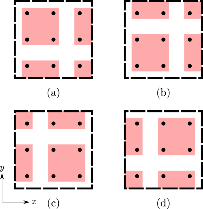
Furthermore, we assume that $\tilde{U}$ can be efficiently approximated by a four-layer quantum circuit $U^{\prime}$of the form of Fig. 1, where each unitary acts on plaquettes of $\ell\times\ell$ sites. For that, we have to require that $\ell=c^{\prime}N^{\nu}$ with $c^{\prime}>0$ and $\mu<\nu<1$ such that the range of all unitaries is much larger than the longest localization length $\xi_{\mathrm{max}}$ in the limit of large $N$ Wahl et al. (2017). With increasing $N$, the quantum circuit $U^{\prime}$ thus approximates $\tilde{U}$ with arbitrary accuracy Chan and Wahl (2020). In order to describe the topological properties of MBL systems within time scales of order Eq. (8), it thus suffices to characterize quantum circuits of the type $U^{\prime}$.

Our approach towards the classification of SPT phases differs from the one more commonly found in the literature, where quantum circuits are assumed to have fixed gate length and whose depth is variable, albeit independent of the system size. In contrast, we (i) keep the number of layers constant at four and have a flexible gate length, which (ii) is allowed to grow sublinearly with the system size. The reasons for this modified approach are as follows: (i) MBL systems with true random disorder contain regions of anomalously small disorder. The localization length $\xi_{i}$ of a LIOM located in the center of such an anomalous region has to be of the order of its size. Since such a “thermal puddle” is featureless, the quantum circuit should have of the order of $2^{\xi_{i}^{2}}$ parameters in that region to be able to diagonalize the Hamiltonian with any reasonable accuracy Wahl et al. (2017). To that end, one could increase the depth of the quantum circuit exponentially with $\xi_{i}^{2}$, or the length $\ell$ of its gates linearly with $\xi_{i}$. Hence, a quantum circuit with long gates is the more natural choice for MBL systems. There is no need to increase the depth of the quantum circuit as well, cf. Ref. Wahl et al., 2017. (ii) The gate length has to increase with the system size, since the maximum $\xi_{i}$ does: In the thermodynamic limit, there will be anomalous regions of arbitrarily large size, since there is a finite probability for them to occur. Thus, $\xi_{\mathrm{max}}=\max_{i}(\xi_{i})$ diverges in the thermodynamic limit. Therefore, $\ell$ also has to grow with the system size in order to allow for a correct global description of any reasonable accuracy.

The classification we derive below is based on the question whether such quantum circuits with a diverging gate length can be continuously connected. Consequently, our results also apply to all more restrictive sets of quantum circuits: The central result of our work is that for given gate length $\ell$ the whole set $\mathcal{S}$ of four-layer quantum circuits with a symmetry decomposes into disconnected sets $\mathcal{S}_{a}$ given by the third cohomology class $a$ of the symmetry group, $S=\cup_{a}S_{a}$. A quantum circuit contained in $\mathcal{S}_{a}$ cannot be continuously connected with a quantum circuit contained in $\mathcal{S}_{b}$ for $a\neq b$. Now consider a more restrictive notion of quantum circuits $\mathcal{R}$ contained in $\mathcal{S}$, $\mathcal{R}\subset\mathcal{S}$. As long as this more restrictive set contains a representative of each cohomology class $a$, the same decomposition has to apply, i.e., $\mathcal{R}=\cup_{a}\mathcal{R}_{a}$, $\mathcal{R}_{a}\neq\{\}$ and $\mathcal{R}_{a}\subseteq\mathcal{S}_{a}$. The last relation implies likewise that quantum circuits contained in $\mathcal{R}_{a}$ and $\mathcal{R}_{b}$ cannot be continuously connected for $a\neq b$. An example of such a more restrictive set $\mathcal{R}$ is the commonly used quantum circuits with a large but fixed number of layers and (small) fixed gate length Bauer and Nayak (2013): Those quantum circuits have strict short-range correlations and can thus be approximated with arbitrarily small error by our ansatz if $\ell$ is sufficiently large. (In one dimension, multi-layer quantum circuits can even be written exactly as two-layer long-gate ones.) Furthermore, those more restrictive quantum circuits have a representative in each cohomology class: Such a representative is the finite-depth, finite-gate-length quantum circuit which maps a product state to a ground state in the corresponding SPT phase.

The quantum circuit $U^{\prime}$ is the natural generalization of the two-layer quantum circuit with long gates used in one dimension to represent MBL systems Wahl et al. (2017); Wahl (2018); Chan and Wahl (2020): It consists of parallel one-dimensional two-layer quantum circuits, which are themselves coupled with each other in a two-layer quantum circuit structure,

[Uncaptioned image].[Uncaptioned image]\includegraphics[width=390.25534pt,valign={c}]{2019_07_QC_UV.pdf}\;. (19)

Here, we blocked together sites as in Fig. 1, i.e., each tensor leg corresponds to $\frac{\ell}{2}\times\frac{\ell}{2}$ sites. The unitaries of $U_{k}$ are located in the first two layers of Fig. 1 (i.e, Fig. 1a,b), the unitaries of $V_{k}$ in the second two layers (Fig. 1c,d). For the derivation below we assume that one-dimensional unitaries which encode states with strict short-range entanglement can be efficiently approximated by one-dimensional two-layer quantum circuits with long gates, which corresponds to the assumption that one-dimensional MBL systems can be efficiently approximated by such unitaries Wahl et al. (2017); Wahl (2018); Chan and Wahl (2020).

III.2 Main results

$U^{\prime}$ (we will drop the prime symbol from now on) approximately fulfills Eq. (18), as it approximately diagonalizes the Hamiltonian $H$. It follows from Eqs. (18) and (19) that $\Theta_{g}$ can likewise be written as a four-layer quantum circuit (see Sec. IV.1.1 for details), thus making Eq. (18) an equality of two short-depth quantum circuits.

Refer to caption
Figure 1: An illustration of the 4-layer quantum circuit approximating the unitary $\tilde{U}$. The $xy$-plane is parallel to the plane where the sites of the system are located. The unitaries are stacked from bottom to top in the order (a), (b), (c), (d) (parallel to the $z$-axis). (a) represents the top view of the first layer, (b) of the second layer, and so on. A dot represents a group of $\frac{\ell}{2}\times\frac{\ell}{2}$ sites. A red box represents a unitary. The quantum circuit periodically extends beyond the region defined by the dashed lines.

Next, we perform manipulations with the quantum circuits. We collapse the quantum circuits of Eq. (18) along the $y$-direction, so that (18) becomes an equality of two one-dimensional quantum circuits, which are stretched out along the $x$-direction. One obtains

[Uncaptioned image],[Uncaptioned image]\displaystyle\includegraphics[width=390.25534pt,valign={c}]{2019_07_draw4_v2.eps}\;, (20)

where $g$ represents $\mathpzc{v}_{g}^{\otimes N\ell/2}$, and the $\Theta^{g}_{j}$ are (diagonal) unitaries extended along the $y$-direction. They constitute the quantum circuit representation of $\Theta_{g}$. This equation is of the general form (see red dashed lines)

U1′′U2′′Un′′V1′′V2′′Vn′′Vn′′=U1U2UnV1V2VnVn.superscriptsubscript𝑈1′′superscriptsubscript𝑈2′′superscriptsubscript𝑈𝑛′′superscriptsubscript𝑉1′′superscriptsubscript𝑉2′′superscriptsubscript𝑉𝑛′′superscriptsubscript𝑉𝑛′′superscriptsubscript𝑈1superscriptsubscript𝑈2superscriptsubscript𝑈𝑛superscriptsubscript𝑉1superscriptsubscript𝑉2superscriptsubscript𝑉𝑛superscriptsubscript𝑉𝑛\leavevmode\hbox to241.87pt{\vbox to151.03pt{\pgfpicture\makeatletter\hbox{\hskip 62.39655pt\lower-106.81415pt\hbox to0.0pt{\pgfsys@beginscope\pgfsys@invoke{ }\definecolor{pgfstrokecolor}{rgb}{0,0,0}\pgfsys@color@rgb@stroke{0}{0}{0}\pgfsys@invoke{ }\pgfsys@color@rgb@fill{0}{0}{0}\pgfsys@invoke{ }\pgfsys@setlinewidth{0.4pt}\pgfsys@invoke{ }\nullfont\hbox to0.0pt{\pgfsys@beginscope\pgfsys@invoke{ }{{}} {}{{}}{} {}{}\pgfsys@beginscope\pgfsys@invoke{ }\pgfsys@setlinewidth{0.8pt}\pgfsys@invoke{ }{}\pgfsys@moveto{-12.51907pt}{-18.7791pt}\pgfsys@lineto{-12.51907pt}{43.81728pt}\pgfsys@stroke\pgfsys@invoke{ } \pgfsys@invoke{\lxSVG@closescope }\pgfsys@endscope{}{{}}{} {}{}\pgfsys@beginscope\pgfsys@invoke{ }\pgfsys@setlinewidth{0.8pt}\pgfsys@invoke{ }{}\pgfsys@moveto{12.51907pt}{-18.7791pt}\pgfsys@lineto{12.51907pt}{43.81728pt}\pgfsys@stroke\pgfsys@invoke{ } \pgfsys@invoke{\lxSVG@closescope }\pgfsys@endscope{}{{}}{} {}{{}}{}{}{}{}{{}}{}\pgfsys@beginscope\pgfsys@invoke{ }\pgfsys@setlinewidth{0.8pt}\pgfsys@invoke{ }\definecolor[named]{pgffillcolor}{rgb}{1,1,1}\pgfsys@color@gray@fill{1}\pgfsys@invoke{ }{}\pgfsys@moveto{-12.51907pt}{-7.82454pt}\pgfsys@moveto{-12.51907pt}{-7.82454pt}\pgfsys@lineto{-12.51907pt}{7.82454pt}\pgfsys@lineto{12.51907pt}{7.82454pt}\pgfsys@lineto{12.51907pt}{-7.82454pt}\pgfsys@closepath\pgfsys@moveto{12.51907pt}{7.82454pt}\pgfsys@fillstroke\pgfsys@invoke{ } \pgfsys@invoke{\lxSVG@closescope }\pgfsys@endscope {}{{}}{} {}{}\pgfsys@beginscope\pgfsys@invoke{ }\pgfsys@setlinewidth{0.8pt}\pgfsys@invoke{ }{}\pgfsys@moveto{37.55774pt}{-18.7791pt}\pgfsys@lineto{37.55774pt}{43.81728pt}\pgfsys@stroke\pgfsys@invoke{ } \pgfsys@invoke{\lxSVG@closescope }\pgfsys@endscope{}{{}}{} {}{}\pgfsys@beginscope\pgfsys@invoke{ }\pgfsys@setlinewidth{0.8pt}\pgfsys@invoke{ }{}\pgfsys@moveto{62.5964pt}{-18.7791pt}\pgfsys@lineto{62.5964pt}{43.81728pt}\pgfsys@stroke\pgfsys@invoke{ } \pgfsys@invoke{\lxSVG@closescope }\pgfsys@endscope{}{{}}{} {}{{}}{}{}{}{}{{}}{}\pgfsys@beginscope\pgfsys@invoke{ }\pgfsys@setlinewidth{0.8pt}\pgfsys@invoke{ }\definecolor[named]{pgffillcolor}{rgb}{1,1,1}\pgfsys@color@gray@fill{1}\pgfsys@invoke{ }{}\pgfsys@moveto{37.55774pt}{-7.82454pt}\pgfsys@moveto{37.55774pt}{-7.82454pt}\pgfsys@lineto{37.55774pt}{7.82454pt}\pgfsys@lineto{62.5964pt}{7.82454pt}\pgfsys@lineto{62.5964pt}{-7.82454pt}\pgfsys@closepath\pgfsys@moveto{62.5964pt}{7.82454pt}\pgfsys@fillstroke\pgfsys@invoke{ } \pgfsys@invoke{\lxSVG@closescope }\pgfsys@endscope {}{{}}{} {}{}\pgfsys@beginscope\pgfsys@invoke{ }\pgfsys@setlinewidth{0.8pt}\pgfsys@invoke{ }{}\pgfsys@moveto{87.63506pt}{-18.7791pt}\pgfsys@lineto{87.63506pt}{43.81728pt}\pgfsys@stroke\pgfsys@invoke{ } \pgfsys@invoke{\lxSVG@closescope }\pgfsys@endscope{}{{}}{} {}{}\pgfsys@beginscope\pgfsys@invoke{ }\pgfsys@setlinewidth{0.8pt}\pgfsys@invoke{ }{}\pgfsys@moveto{112.67372pt}{-18.7791pt}\pgfsys@lineto{112.67372pt}{43.81728pt}\pgfsys@stroke\pgfsys@invoke{ } \pgfsys@invoke{\lxSVG@closescope }\pgfsys@endscope{}{{}}{} {}{{}}{}{}{}{}{{}}{}\pgfsys@beginscope\pgfsys@invoke{ }\pgfsys@setlinewidth{0.8pt}\pgfsys@invoke{ }\definecolor[named]{pgffillcolor}{rgb}{1,1,1}\pgfsys@color@gray@fill{1}\pgfsys@invoke{ }{}\pgfsys@moveto{87.63506pt}{-7.82454pt}\pgfsys@moveto{87.63506pt}{-7.82454pt}\pgfsys@lineto{87.63506pt}{7.82454pt}\pgfsys@lineto{112.67372pt}{7.82454pt}\pgfsys@lineto{112.67372pt}{-7.82454pt}\pgfsys@closepath\pgfsys@moveto{112.67372pt}{7.82454pt}\pgfsys@fillstroke\pgfsys@invoke{ } \pgfsys@invoke{\lxSVG@closescope }\pgfsys@endscope {}{{}}{} {}{}\pgfsys@beginscope\pgfsys@invoke{ }\pgfsys@setlinewidth{0.8pt}\pgfsys@invoke{ }{}\pgfsys@moveto{137.71191pt}{-18.7791pt}\pgfsys@lineto{137.71191pt}{43.81728pt}\pgfsys@stroke\pgfsys@invoke{ } \pgfsys@invoke{\lxSVG@closescope }\pgfsys@endscope{}{{}}{} {}{}\pgfsys@beginscope\pgfsys@invoke{ }\pgfsys@setlinewidth{0.8pt}\pgfsys@invoke{ }{}\pgfsys@moveto{162.75058pt}{-18.7791pt}\pgfsys@lineto{162.75058pt}{43.81728pt}\pgfsys@stroke\pgfsys@invoke{ } \pgfsys@invoke{\lxSVG@closescope }\pgfsys@endscope{}{{}}{} {}{{}}{}{}{}{}{{}}{}\pgfsys@beginscope\pgfsys@invoke{ }\pgfsys@setlinewidth{0.8pt}\pgfsys@invoke{ }\definecolor[named]{pgffillcolor}{rgb}{1,1,1}\pgfsys@color@gray@fill{1}\pgfsys@invoke{ }{}\pgfsys@moveto{137.71191pt}{-7.82454pt}\pgfsys@moveto{137.71191pt}{-7.82454pt}\pgfsys@lineto{137.71191pt}{7.82454pt}\pgfsys@lineto{162.75058pt}{7.82454pt}\pgfsys@lineto{162.75058pt}{-7.82454pt}\pgfsys@closepath\pgfsys@moveto{162.75058pt}{7.82454pt}\pgfsys@fillstroke\pgfsys@invoke{ } \pgfsys@invoke{\lxSVG@closescope }\pgfsys@endscope {}{{}}{} {}{{}}{}{}{}{}{{}}{}\pgfsys@beginscope\pgfsys@invoke{ }\pgfsys@setlinewidth{0.8pt}\pgfsys@invoke{ }\definecolor[named]{pgffillcolor}{rgb}{1,1,1}\pgfsys@color@gray@fill{1}\pgfsys@invoke{ }{}\pgfsys@moveto{12.51907pt}{17.2141pt}\pgfsys@moveto{12.51907pt}{17.2141pt}\pgfsys@lineto{12.51907pt}{32.86319pt}\pgfsys@lineto{37.55774pt}{32.86319pt}\pgfsys@lineto{37.55774pt}{17.2141pt}\pgfsys@closepath\pgfsys@moveto{37.55774pt}{32.86319pt}\pgfsys@fillstroke\pgfsys@invoke{ } \pgfsys@invoke{\lxSVG@closescope }\pgfsys@endscope {}{{}}{} {}{{}}{}{}{}{}{{}}{}\pgfsys@beginscope\pgfsys@invoke{ }\pgfsys@setlinewidth{0.8pt}\pgfsys@invoke{ }\definecolor[named]{pgffillcolor}{rgb}{1,1,1}\pgfsys@color@gray@fill{1}\pgfsys@invoke{ }{}\pgfsys@moveto{62.5964pt}{17.2141pt}\pgfsys@moveto{62.5964pt}{17.2141pt}\pgfsys@lineto{62.5964pt}{32.86319pt}\pgfsys@lineto{87.63506pt}{32.86319pt}\pgfsys@lineto{87.63506pt}{17.2141pt}\pgfsys@closepath\pgfsys@moveto{87.63506pt}{32.86319pt}\pgfsys@fillstroke\pgfsys@invoke{ } \pgfsys@invoke{\lxSVG@closescope }\pgfsys@endscope {}{{}}{} {}{{}}{}{}{}{}{{}}{}\pgfsys@beginscope\pgfsys@invoke{ }\pgfsys@setlinewidth{0.8pt}\pgfsys@invoke{ }\definecolor[named]{pgffillcolor}{rgb}{1,1,1}\pgfsys@color@gray@fill{1}\pgfsys@invoke{ }{}\pgfsys@moveto{112.67372pt}{17.2141pt}\pgfsys@moveto{112.67372pt}{17.2141pt}\pgfsys@lineto{112.67372pt}{32.86319pt}\pgfsys@lineto{137.71191pt}{32.86319pt}\pgfsys@lineto{137.71191pt}{17.2141pt}\pgfsys@closepath\pgfsys@moveto{137.71191pt}{32.86319pt}\pgfsys@fillstroke\pgfsys@invoke{ } \pgfsys@invoke{\lxSVG@closescope }\pgfsys@endscope {}{{}}{} {}{} {}{} {}{}\pgfsys@beginscope\pgfsys@invoke{ }\pgfsys@setlinewidth{0.8pt}\pgfsys@invoke{ }{}\pgfsys@moveto{-25.03865pt}{17.2141pt}\pgfsys@lineto{-12.51907pt}{17.2141pt}\pgfsys@lineto{-12.51907pt}{32.86319pt}\pgfsys@lineto{-25.03865pt}{32.86319pt}\pgfsys@stroke\pgfsys@invoke{ } \pgfsys@invoke{\lxSVG@closescope }\pgfsys@endscope{}{{}}{} {}{} {}{} {}{}\pgfsys@beginscope\pgfsys@invoke{ }\pgfsys@setlinewidth{0.8pt}\pgfsys@invoke{ }{}\pgfsys@moveto{175.27014pt}{17.2141pt}\pgfsys@lineto{162.75058pt}{17.2141pt}\pgfsys@lineto{162.75058pt}{32.86319pt}\pgfsys@lineto{175.27014pt}{32.86319pt}\pgfsys@stroke\pgfsys@invoke{ } \pgfsys@invoke{\lxSVG@closescope }\pgfsys@endscope{}{{}} {{{}{}}}{{{}}}{{}}{{}}\hbox{\hbox{\hbox{{\pgfsys@beginscope\pgfsys@invoke{ }{{}{{}}{}{}} \pgfsys@invoke{\lxSVG@closescope }\pgfsys@endscope}}}\hbox{{\pgfsys@beginscope\pgfsys@invoke{ }{{}{}{{ {}{}}}{ {}{}} {{}{{}}}{{}{}}{}{{}{}} { }{{{{}}\pgfsys@beginscope\pgfsys@invoke{ }\pgfsys@transformcm{1.0}{0.0}{0.0}{1.0}{-5.85655pt}{-3.2922pt}\pgfsys@invoke{ }\hbox{{\definecolor{pgfstrokecolor}{rgb}{0,0,0}\pgfsys@color@rgb@stroke{0}{0}{0}\pgfsys@invoke{ }\pgfsys@color@rgb@fill{0}{0}{0}\pgfsys@invoke{ }\hbox{{$U_{1}^{\prime\prime}$}} }}\pgfsys@invoke{\lxSVG@closescope }\pgfsys@endscope}}} \pgfsys@invoke{\lxSVG@closescope }\pgfsys@endscope}}} {}{{}} {{{}{}}}{{{}}}{{}}{{}}\hbox{\hbox{\hbox{{\pgfsys@beginscope\pgfsys@invoke{ }{{}{{}}{}{}} \pgfsys@invoke{\lxSVG@closescope }\pgfsys@endscope}}}\hbox{{\pgfsys@beginscope\pgfsys@invoke{ }{{}{}{{ {}{}}}{ {}{}} {{}{{}}}{{}{}}{}{{}{}} { }{{{{}}\pgfsys@beginscope\pgfsys@invoke{ }\pgfsys@transformcm{1.0}{0.0}{0.0}{1.0}{44.22084pt}{-3.2922pt}\pgfsys@invoke{ }\hbox{{\definecolor{pgfstrokecolor}{rgb}{0,0,0}\pgfsys@color@rgb@stroke{0}{0}{0}\pgfsys@invoke{ }\pgfsys@color@rgb@fill{0}{0}{0}\pgfsys@invoke{ }\hbox{{$U_{2}^{\prime\prime}$}} }}\pgfsys@invoke{\lxSVG@closescope }\pgfsys@endscope}}} \pgfsys@invoke{\lxSVG@closescope }\pgfsys@endscope}}} {}{{}} {{{}{}}}{{{}}}{{}}{{}}\hbox{\hbox{\hbox{{\pgfsys@beginscope\pgfsys@invoke{ }{{}{{}}{}{}} \pgfsys@invoke{\lxSVG@closescope }\pgfsys@endscope}}}\hbox{{\pgfsys@beginscope\pgfsys@invoke{ }{{}{}{{ {}{}}}{ {}{}} {{}{{}}}{{}{}}{}{{}{}} { }{{{{}}\pgfsys@beginscope\pgfsys@invoke{ }\pgfsys@transformcm{1.0}{0.0}{0.0}{1.0}{94.29782pt}{-2.5pt}\pgfsys@invoke{ }\hbox{{\definecolor{pgfstrokecolor}{rgb}{0,0,0}\pgfsys@color@rgb@stroke{0}{0}{0}\pgfsys@invoke{ }\pgfsys@color@rgb@fill{0}{0}{0}\pgfsys@invoke{ }\hbox{{$\ldots$}} }}\pgfsys@invoke{\lxSVG@closescope }\pgfsys@endscope}}} \pgfsys@invoke{\lxSVG@closescope }\pgfsys@endscope}}} {}{{}} {{{}{}}}{{{}}}{{}}{{}}\hbox{\hbox{\hbox{{\pgfsys@beginscope\pgfsys@invoke{ }{{}{{}}{}{}} \pgfsys@invoke{\lxSVG@closescope }\pgfsys@endscope}}}\hbox{{\pgfsys@beginscope\pgfsys@invoke{ }{{}{}{{ {}{}}}{ {}{}} {{}{{}}}{{}{}}{}{{}{}} { }{{{{}}\pgfsys@beginscope\pgfsys@invoke{ }\pgfsys@transformcm{1.0}{0.0}{0.0}{1.0}{144.37527pt}{-3.59166pt}\pgfsys@invoke{ }\hbox{{\definecolor{pgfstrokecolor}{rgb}{0,0,0}\pgfsys@color@rgb@stroke{0}{0}{0}\pgfsys@invoke{ }\pgfsys@color@rgb@fill{0}{0}{0}\pgfsys@invoke{ }\hbox{{$U_{n}^{\prime\prime}$}} }}\pgfsys@invoke{\lxSVG@closescope }\pgfsys@endscope}}} \pgfsys@invoke{\lxSVG@closescope }\pgfsys@endscope}}} {}{{}} {{{}{}}}{{{}}}{{}}{{}}\hbox{\hbox{\hbox{{\pgfsys@beginscope\pgfsys@invoke{ }{{}{{}}{}{}} \pgfsys@invoke{\lxSVG@closescope }\pgfsys@endscope}}}\hbox{{\pgfsys@beginscope\pgfsys@invoke{ }{{}{}{{ {}{}}}{ {}{}} {{}{{}}}{{}{}}{}{{}{}} { }{{{{}}\pgfsys@beginscope\pgfsys@invoke{ }\pgfsys@transformcm{1.0}{0.0}{0.0}{1.0}{19.18211pt}{21.74649pt}\pgfsys@invoke{ }\hbox{{\definecolor{pgfstrokecolor}{rgb}{0,0,0}\pgfsys@color@rgb@stroke{0}{0}{0}\pgfsys@invoke{ }\pgfsys@color@rgb@fill{0}{0}{0}\pgfsys@invoke{ }\hbox{{$V_{1}^{\prime\prime}$}} }}\pgfsys@invoke{\lxSVG@closescope }\pgfsys@endscope}}} \pgfsys@invoke{\lxSVG@closescope }\pgfsys@endscope}}} {}{{}} {{{}{}}}{{{}}}{{}}{{}}\hbox{\hbox{\hbox{{\pgfsys@beginscope\pgfsys@invoke{ }{{}{{}}{}{}} \pgfsys@invoke{\lxSVG@closescope }\pgfsys@endscope}}}\hbox{{\pgfsys@beginscope\pgfsys@invoke{ }{{}{}{{ {}{}}}{ {}{}} {{}{{}}}{{}{}}{}{{}{}} { }{{{{}}\pgfsys@beginscope\pgfsys@invoke{ }\pgfsys@transformcm{1.0}{0.0}{0.0}{1.0}{69.25957pt}{21.74649pt}\pgfsys@invoke{ }\hbox{{\definecolor{pgfstrokecolor}{rgb}{0,0,0}\pgfsys@color@rgb@stroke{0}{0}{0}\pgfsys@invoke{ }\pgfsys@color@rgb@fill{0}{0}{0}\pgfsys@invoke{ }\hbox{{$V_{2}^{\prime\prime}$}} }}\pgfsys@invoke{\lxSVG@closescope }\pgfsys@endscope}}} \pgfsys@invoke{\lxSVG@closescope }\pgfsys@endscope}}} {}{{}} {{{}{}}}{{{}}}{{}}{{}}\hbox{\hbox{\hbox{{\pgfsys@beginscope\pgfsys@invoke{ }{{}{{}}{}{}} \pgfsys@invoke{\lxSVG@closescope }\pgfsys@endscope}}}\hbox{{\pgfsys@beginscope\pgfsys@invoke{ }{{}{}{{ {}{}}}{ {}{}} {{}{{}}}{{}{}}{}{{}{}} { }{{{{}}\pgfsys@beginscope\pgfsys@invoke{ }\pgfsys@transformcm{1.0}{0.0}{0.0}{1.0}{119.33655pt}{22.5387pt}\pgfsys@invoke{ }\hbox{{\definecolor{pgfstrokecolor}{rgb}{0,0,0}\pgfsys@color@rgb@stroke{0}{0}{0}\pgfsys@invoke{ }\pgfsys@color@rgb@fill{0}{0}{0}\pgfsys@invoke{ }\hbox{{$\ldots$}} }}\pgfsys@invoke{\lxSVG@closescope }\pgfsys@endscope}}} \pgfsys@invoke{\lxSVG@closescope }\pgfsys@endscope}}} {}{{}} {{{}{}}}{{{}}}{{}}{{}}\hbox{\hbox{\hbox{{\pgfsys@beginscope\pgfsys@invoke{ }{{}{{}}{}{}} \pgfsys@invoke{\lxSVG@closescope }\pgfsys@endscope}}}\hbox{{\pgfsys@beginscope\pgfsys@invoke{ }{{}{}{{ {}{}}}{ {}{}} {{}{{}}}{{}{}}{}{{}{}} { }{{{{}}\pgfsys@beginscope\pgfsys@invoke{ }\pgfsys@transformcm{1.0}{0.0}{0.0}{1.0}{164.71895pt}{20.82094pt}\pgfsys@invoke{ }\hbox{{\definecolor{pgfstrokecolor}{rgb}{0,0,0}\pgfsys@color@rgb@stroke{0}{0}{0}\pgfsys@invoke{ }\pgfsys@color@rgb@fill{0}{0}{0}\pgfsys@invoke{ }\hbox{{$V_{n}^{\prime\prime}$}} }}\pgfsys@invoke{\lxSVG@closescope }\pgfsys@endscope}}} \pgfsys@invoke{\lxSVG@closescope }\pgfsys@endscope}}} {}{{}} {{{}{}}}{{{}}}{{}}{{}}\hbox{\hbox{\hbox{{\pgfsys@beginscope\pgfsys@invoke{ }{{}{{}}{}{}} \pgfsys@invoke{\lxSVG@closescope }\pgfsys@endscope}}}\hbox{{\pgfsys@beginscope\pgfsys@invoke{ }{{}{}{{ {}{}}}{ {}{}} {{}{{}}}{{}{}}{}{{}{}} { }{{{{}}\pgfsys@beginscope\pgfsys@invoke{ }\pgfsys@transformcm{1.0}{0.0}{0.0}{1.0}{-27.76526pt}{20.82094pt}\pgfsys@invoke{ }\hbox{{\definecolor{pgfstrokecolor}{rgb}{0,0,0}\pgfsys@color@rgb@stroke{0}{0}{0}\pgfsys@invoke{ }\pgfsys@color@rgb@fill{0}{0}{0}\pgfsys@invoke{ }\hbox{{$V_{n}^{\prime\prime}$}} }}\pgfsys@invoke{\lxSVG@closescope }\pgfsys@endscope}}} \pgfsys@invoke{\lxSVG@closescope }\pgfsys@endscope}}} \par\pgfsys@beginscope\pgfsys@invoke{ }{{}} {}{{}} {{{}{}}}{{{}}}{{}}{{}}\hbox{\hbox{\hbox{{\pgfsys@beginscope\pgfsys@invoke{ }{{}{{}}{}{}} \pgfsys@invoke{\lxSVG@closescope }\pgfsys@endscope}}}\hbox{{\pgfsys@beginscope\pgfsys@invoke{ }{{}{}{{ {}{}}}{ {}{}} {{}{{}}}{{}{}}{}{{}{}} { }{{{{}}\pgfsys@beginscope\pgfsys@invoke{ }\pgfsys@transformcm{1.0}{0.0}{0.0}{1.0}{-59.06354pt}{-64.43071pt}\pgfsys@invoke{ }\hbox{{\definecolor{pgfstrokecolor}{rgb}{0,0,0}\pgfsys@color@rgb@stroke{0}{0}{0}\pgfsys@invoke{ }\pgfsys@color@rgb@fill{0}{0}{0}\pgfsys@invoke{ }\hbox{{${=}$}} }}\pgfsys@invoke{\lxSVG@closescope }\pgfsys@endscope}}} \pgfsys@invoke{\lxSVG@closescope }\pgfsys@endscope}}} {}{{}}{} {}{}\pgfsys@beginscope\pgfsys@invoke{ }\pgfsys@setlinewidth{0.8pt}\pgfsys@invoke{ }{}\pgfsys@moveto{-12.51907pt}{-106.41415pt}\pgfsys@lineto{-12.51907pt}{-43.81778pt}\pgfsys@stroke\pgfsys@invoke{ } \pgfsys@invoke{\lxSVG@closescope }\pgfsys@endscope{}{{}}{} {}{}\pgfsys@beginscope\pgfsys@invoke{ }\pgfsys@setlinewidth{0.8pt}\pgfsys@invoke{ }{}\pgfsys@moveto{12.51907pt}{-106.41415pt}\pgfsys@lineto{12.51907pt}{-43.81778pt}\pgfsys@stroke\pgfsys@invoke{ } \pgfsys@invoke{\lxSVG@closescope }\pgfsys@endscope{}{{}}{} {}{{}}{}{}{}{}{{}}{}\pgfsys@beginscope\pgfsys@invoke{ }\pgfsys@setlinewidth{0.8pt}\pgfsys@invoke{ }\definecolor[named]{pgffillcolor}{rgb}{1,1,1}\pgfsys@color@gray@fill{1}\pgfsys@invoke{ }{}\pgfsys@moveto{-12.51907pt}{-95.4596pt}\pgfsys@moveto{-12.51907pt}{-95.4596pt}\pgfsys@lineto{-12.51907pt}{-79.81052pt}\pgfsys@lineto{12.51907pt}{-79.81052pt}\pgfsys@lineto{12.51907pt}{-95.4596pt}\pgfsys@closepath\pgfsys@moveto{12.51907pt}{-79.81052pt}\pgfsys@fillstroke\pgfsys@invoke{ } \pgfsys@invoke{\lxSVG@closescope }\pgfsys@endscope {}{{}}{} {}{}\pgfsys@beginscope\pgfsys@invoke{ }\pgfsys@setlinewidth{0.8pt}\pgfsys@invoke{ }{}\pgfsys@moveto{37.55774pt}{-106.41415pt}\pgfsys@lineto{37.55774pt}{-43.81778pt}\pgfsys@stroke\pgfsys@invoke{ } \pgfsys@invoke{\lxSVG@closescope }\pgfsys@endscope{}{{}}{} {}{}\pgfsys@beginscope\pgfsys@invoke{ }\pgfsys@setlinewidth{0.8pt}\pgfsys@invoke{ }{}\pgfsys@moveto{62.5964pt}{-106.41415pt}\pgfsys@lineto{62.5964pt}{-43.81778pt}\pgfsys@stroke\pgfsys@invoke{ } \pgfsys@invoke{\lxSVG@closescope }\pgfsys@endscope{}{{}}{} {}{{}}{}{}{}{}{{}}{}\pgfsys@beginscope\pgfsys@invoke{ }\pgfsys@setlinewidth{0.8pt}\pgfsys@invoke{ }\definecolor[named]{pgffillcolor}{rgb}{1,1,1}\pgfsys@color@gray@fill{1}\pgfsys@invoke{ }{}\pgfsys@moveto{37.55774pt}{-95.4596pt}\pgfsys@moveto{37.55774pt}{-95.4596pt}\pgfsys@lineto{37.55774pt}{-79.81052pt}\pgfsys@lineto{62.5964pt}{-79.81052pt}\pgfsys@lineto{62.5964pt}{-95.4596pt}\pgfsys@closepath\pgfsys@moveto{62.5964pt}{-79.81052pt}\pgfsys@fillstroke\pgfsys@invoke{ } \pgfsys@invoke{\lxSVG@closescope }\pgfsys@endscope {}{{}}{} {}{}\pgfsys@beginscope\pgfsys@invoke{ }\pgfsys@setlinewidth{0.8pt}\pgfsys@invoke{ }{}\pgfsys@moveto{87.63506pt}{-106.41415pt}\pgfsys@lineto{87.63506pt}{-43.81778pt}\pgfsys@stroke\pgfsys@invoke{ } \pgfsys@invoke{\lxSVG@closescope }\pgfsys@endscope{}{{}}{} {}{}\pgfsys@beginscope\pgfsys@invoke{ }\pgfsys@setlinewidth{0.8pt}\pgfsys@invoke{ }{}\pgfsys@moveto{112.67372pt}{-106.41415pt}\pgfsys@lineto{112.67372pt}{-43.81778pt}\pgfsys@stroke\pgfsys@invoke{ } \pgfsys@invoke{\lxSVG@closescope }\pgfsys@endscope{}{{}}{} {}{{}}{}{}{}{}{{}}{}\pgfsys@beginscope\pgfsys@invoke{ }\pgfsys@setlinewidth{0.8pt}\pgfsys@invoke{ }\definecolor[named]{pgffillcolor}{rgb}{1,1,1}\pgfsys@color@gray@fill{1}\pgfsys@invoke{ }{}\pgfsys@moveto{87.63506pt}{-95.4596pt}\pgfsys@moveto{87.63506pt}{-95.4596pt}\pgfsys@lineto{87.63506pt}{-79.81052pt}\pgfsys@lineto{112.67372pt}{-79.81052pt}\pgfsys@lineto{112.67372pt}{-95.4596pt}\pgfsys@closepath\pgfsys@moveto{112.67372pt}{-79.81052pt}\pgfsys@fillstroke\pgfsys@invoke{ } \pgfsys@invoke{\lxSVG@closescope }\pgfsys@endscope {}{{}}{} {}{}\pgfsys@beginscope\pgfsys@invoke{ }\pgfsys@setlinewidth{0.8pt}\pgfsys@invoke{ }{}\pgfsys@moveto{137.71191pt}{-106.41415pt}\pgfsys@lineto{137.71191pt}{-43.81778pt}\pgfsys@stroke\pgfsys@invoke{ } \pgfsys@invoke{\lxSVG@closescope }\pgfsys@endscope{}{{}}{} {}{}\pgfsys@beginscope\pgfsys@invoke{ }\pgfsys@setlinewidth{0.8pt}\pgfsys@invoke{ }{}\pgfsys@moveto{162.75058pt}{-106.41415pt}\pgfsys@lineto{162.75058pt}{-43.81778pt}\pgfsys@stroke\pgfsys@invoke{ } \pgfsys@invoke{\lxSVG@closescope }\pgfsys@endscope{}{{}}{} {}{{}}{}{}{}{}{{}}{}\pgfsys@beginscope\pgfsys@invoke{ }\pgfsys@setlinewidth{0.8pt}\pgfsys@invoke{ }\definecolor[named]{pgffillcolor}{rgb}{1,1,1}\pgfsys@color@gray@fill{1}\pgfsys@invoke{ }{}\pgfsys@moveto{137.71191pt}{-95.4596pt}\pgfsys@moveto{137.71191pt}{-95.4596pt}\pgfsys@lineto{137.71191pt}{-79.81052pt}\pgfsys@lineto{162.75058pt}{-79.81052pt}\pgfsys@lineto{162.75058pt}{-95.4596pt}\pgfsys@closepath\pgfsys@moveto{162.75058pt}{-79.81052pt}\pgfsys@fillstroke\pgfsys@invoke{ } \pgfsys@invoke{\lxSVG@closescope }\pgfsys@endscope {}{{}}{} {}{{}}{}{}{}{}{{}}{}\pgfsys@beginscope\pgfsys@invoke{ }\pgfsys@setlinewidth{0.8pt}\pgfsys@invoke{ }\definecolor[named]{pgffillcolor}{rgb}{1,1,1}\pgfsys@color@gray@fill{1}\pgfsys@invoke{ }{}\pgfsys@moveto{12.51907pt}{-70.42096pt}\pgfsys@moveto{12.51907pt}{-70.42096pt}\pgfsys@lineto{12.51907pt}{-54.77187pt}\pgfsys@lineto{37.55774pt}{-54.77187pt}\pgfsys@lineto{37.55774pt}{-70.42096pt}\pgfsys@closepath\pgfsys@moveto{37.55774pt}{-54.77187pt}\pgfsys@fillstroke\pgfsys@invoke{ } \pgfsys@invoke{\lxSVG@closescope }\pgfsys@endscope {}{{}}{} {}{{}}{}{}{}{}{{}}{}\pgfsys@beginscope\pgfsys@invoke{ }\pgfsys@setlinewidth{0.8pt}\pgfsys@invoke{ }\definecolor[named]{pgffillcolor}{rgb}{1,1,1}\pgfsys@color@gray@fill{1}\pgfsys@invoke{ }{}\pgfsys@moveto{62.5964pt}{-70.42096pt}\pgfsys@moveto{62.5964pt}{-70.42096pt}\pgfsys@lineto{62.5964pt}{-54.77187pt}\pgfsys@lineto{87.63506pt}{-54.77187pt}\pgfsys@lineto{87.63506pt}{-70.42096pt}\pgfsys@closepath\pgfsys@moveto{87.63506pt}{-54.77187pt}\pgfsys@fillstroke\pgfsys@invoke{ } \pgfsys@invoke{\lxSVG@closescope }\pgfsys@endscope {}{{}}{} {}{{}}{}{}{}{}{{}}{}\pgfsys@beginscope\pgfsys@invoke{ }\pgfsys@setlinewidth{0.8pt}\pgfsys@invoke{ }\definecolor[named]{pgffillcolor}{rgb}{1,1,1}\pgfsys@color@gray@fill{1}\pgfsys@invoke{ }{}\pgfsys@moveto{112.67372pt}{-70.42096pt}\pgfsys@moveto{112.67372pt}{-70.42096pt}\pgfsys@lineto{112.67372pt}{-54.77187pt}\pgfsys@lineto{137.71191pt}{-54.77187pt}\pgfsys@lineto{137.71191pt}{-70.42096pt}\pgfsys@closepath\pgfsys@moveto{137.71191pt}{-54.77187pt}\pgfsys@fillstroke\pgfsys@invoke{ } \pgfsys@invoke{\lxSVG@closescope }\pgfsys@endscope {}{{}}{} {}{} {}{} {}{}\pgfsys@beginscope\pgfsys@invoke{ }\pgfsys@setlinewidth{0.8pt}\pgfsys@invoke{ }{}\pgfsys@moveto{-25.03865pt}{-70.42096pt}\pgfsys@lineto{-12.51907pt}{-70.42096pt}\pgfsys@lineto{-12.51907pt}{-54.77187pt}\pgfsys@lineto{-25.03865pt}{-54.77187pt}\pgfsys@stroke\pgfsys@invoke{ } \pgfsys@invoke{\lxSVG@closescope }\pgfsys@endscope{}{{}}{} {}{} {}{} {}{}\pgfsys@beginscope\pgfsys@invoke{ }\pgfsys@setlinewidth{0.8pt}\pgfsys@invoke{ }{}\pgfsys@moveto{175.27014pt}{-70.42096pt}\pgfsys@lineto{162.75058pt}{-70.42096pt}\pgfsys@lineto{162.75058pt}{-54.77187pt}\pgfsys@lineto{175.27014pt}{-54.77187pt}\pgfsys@stroke\pgfsys@invoke{ } \pgfsys@invoke{\lxSVG@closescope }\pgfsys@endscope{}{{}} {{{}{}}}{{{}}}{{}}{{}}\hbox{\hbox{\hbox{{\pgfsys@beginscope\pgfsys@invoke{ }{{}{{}}{}{}} \pgfsys@invoke{\lxSVG@closescope }\pgfsys@endscope}}}\hbox{{\pgfsys@beginscope\pgfsys@invoke{ }{{}{}{{ {}{}}}{ {}{}} {{}{{}}}{{}{}}{}{{}{}} { }{{{{}}\pgfsys@beginscope\pgfsys@invoke{ }\pgfsys@transformcm{1.0}{0.0}{0.0}{1.0}{-5.85655pt}{-90.92726pt}\pgfsys@invoke{ }\hbox{{\definecolor{pgfstrokecolor}{rgb}{0,0,0}\pgfsys@color@rgb@stroke{0}{0}{0}\pgfsys@invoke{ }\pgfsys@color@rgb@fill{0}{0}{0}\pgfsys@invoke{ }\hbox{{$U_{1}^{\prime}$}} }}\pgfsys@invoke{\lxSVG@closescope }\pgfsys@endscope}}} \pgfsys@invoke{\lxSVG@closescope }\pgfsys@endscope}}} {}{{}} {{{}{}}}{{{}}}{{}}{{}}\hbox{\hbox{\hbox{{\pgfsys@beginscope\pgfsys@invoke{ }{{}{{}}{}{}} \pgfsys@invoke{\lxSVG@closescope }\pgfsys@endscope}}}\hbox{{\pgfsys@beginscope\pgfsys@invoke{ }{{}{}{{ {}{}}}{ {}{}} {{}{{}}}{{}{}}{}{{}{}} { }{{{{}}\pgfsys@beginscope\pgfsys@invoke{ }\pgfsys@transformcm{1.0}{0.0}{0.0}{1.0}{44.22084pt}{-90.92726pt}\pgfsys@invoke{ }\hbox{{\definecolor{pgfstrokecolor}{rgb}{0,0,0}\pgfsys@color@rgb@stroke{0}{0}{0}\pgfsys@invoke{ }\pgfsys@color@rgb@fill{0}{0}{0}\pgfsys@invoke{ }\hbox{{$U_{2}^{\prime}$}} }}\pgfsys@invoke{\lxSVG@closescope }\pgfsys@endscope}}} \pgfsys@invoke{\lxSVG@closescope }\pgfsys@endscope}}} {}{{}} {{{}{}}}{{{}}}{{}}{{}}\hbox{\hbox{\hbox{{\pgfsys@beginscope\pgfsys@invoke{ }{{}{{}}{}{}} \pgfsys@invoke{\lxSVG@closescope }\pgfsys@endscope}}}\hbox{{\pgfsys@beginscope\pgfsys@invoke{ }{{}{}{{ {}{}}}{ {}{}} {{}{{}}}{{}{}}{}{{}{}} { }{{{{}}\pgfsys@beginscope\pgfsys@invoke{ }\pgfsys@transformcm{1.0}{0.0}{0.0}{1.0}{94.29782pt}{-90.13506pt}\pgfsys@invoke{ }\hbox{{\definecolor{pgfstrokecolor}{rgb}{0,0,0}\pgfsys@color@rgb@stroke{0}{0}{0}\pgfsys@invoke{ }\pgfsys@color@rgb@fill{0}{0}{0}\pgfsys@invoke{ }\hbox{{$\ldots$}} }}\pgfsys@invoke{\lxSVG@closescope }\pgfsys@endscope}}} \pgfsys@invoke{\lxSVG@closescope }\pgfsys@endscope}}} {}{{}} {{{}{}}}{{{}}}{{}}{{}}\hbox{\hbox{\hbox{{\pgfsys@beginscope\pgfsys@invoke{ }{{}{{}}{}{}} \pgfsys@invoke{\lxSVG@closescope }\pgfsys@endscope}}}\hbox{{\pgfsys@beginscope\pgfsys@invoke{ }{{}{}{{ {}{}}}{ {}{}} {{}{{}}}{{}{}}{}{{}{}} { }{{{{}}\pgfsys@beginscope\pgfsys@invoke{ }\pgfsys@transformcm{1.0}{0.0}{0.0}{1.0}{144.37527pt}{-91.22672pt}\pgfsys@invoke{ }\hbox{{\definecolor{pgfstrokecolor}{rgb}{0,0,0}\pgfsys@color@rgb@stroke{0}{0}{0}\pgfsys@invoke{ }\pgfsys@color@rgb@fill{0}{0}{0}\pgfsys@invoke{ }\hbox{{$U_{n}^{\prime}$}} }}\pgfsys@invoke{\lxSVG@closescope }\pgfsys@endscope}}} \pgfsys@invoke{\lxSVG@closescope }\pgfsys@endscope}}} {}{{}} {{{}{}}}{{{}}}{{}}{{}}\hbox{\hbox{\hbox{{\pgfsys@beginscope\pgfsys@invoke{ }{{}{{}}{}{}} \pgfsys@invoke{\lxSVG@closescope }\pgfsys@endscope}}}\hbox{{\pgfsys@beginscope\pgfsys@invoke{ }{{}{}{{ {}{}}}{ {}{}} {{}{{}}}{{}{}}{}{{}{}} { }{{{{}}\pgfsys@beginscope\pgfsys@invoke{ }\pgfsys@transformcm{1.0}{0.0}{0.0}{1.0}{19.18211pt}{-65.88855pt}\pgfsys@invoke{ }\hbox{{\definecolor{pgfstrokecolor}{rgb}{0,0,0}\pgfsys@color@rgb@stroke{0}{0}{0}\pgfsys@invoke{ }\pgfsys@color@rgb@fill{0}{0}{0}\pgfsys@invoke{ }\hbox{{$V_{1}^{\prime}$}} }}\pgfsys@invoke{\lxSVG@closescope }\pgfsys@endscope}}} \pgfsys@invoke{\lxSVG@closescope }\pgfsys@endscope}}} {}{{}} {{{}{}}}{{{}}}{{}}{{}}\hbox{\hbox{\hbox{{\pgfsys@beginscope\pgfsys@invoke{ }{{}{{}}{}{}} \pgfsys@invoke{\lxSVG@closescope }\pgfsys@endscope}}}\hbox{{\pgfsys@beginscope\pgfsys@invoke{ }{{}{}{{ {}{}}}{ {}{}} {{}{{}}}{{}{}}{}{{}{}} { }{{{{}}\pgfsys@beginscope\pgfsys@invoke{ }\pgfsys@transformcm{1.0}{0.0}{0.0}{1.0}{69.25957pt}{-65.88855pt}\pgfsys@invoke{ }\hbox{{\definecolor{pgfstrokecolor}{rgb}{0,0,0}\pgfsys@color@rgb@stroke{0}{0}{0}\pgfsys@invoke{ }\pgfsys@color@rgb@fill{0}{0}{0}\pgfsys@invoke{ }\hbox{{$V_{2}^{\prime}$}} }}\pgfsys@invoke{\lxSVG@closescope }\pgfsys@endscope}}} \pgfsys@invoke{\lxSVG@closescope }\pgfsys@endscope}}} {}{{}} {{{}{}}}{{{}}}{{}}{{}}\hbox{\hbox{\hbox{{\pgfsys@beginscope\pgfsys@invoke{ }{{}{{}}{}{}} \pgfsys@invoke{\lxSVG@closescope }\pgfsys@endscope}}}\hbox{{\pgfsys@beginscope\pgfsys@invoke{ }{{}{}{{ {}{}}}{ {}{}} {{}{{}}}{{}{}}{}{{}{}} { }{{{{}}\pgfsys@beginscope\pgfsys@invoke{ }\pgfsys@transformcm{1.0}{0.0}{0.0}{1.0}{119.33655pt}{-65.09634pt}\pgfsys@invoke{ }\hbox{{\definecolor{pgfstrokecolor}{rgb}{0,0,0}\pgfsys@color@rgb@stroke{0}{0}{0}\pgfsys@invoke{ }\pgfsys@color@rgb@fill{0}{0}{0}\pgfsys@invoke{ }\hbox{{$\ldots$}} }}\pgfsys@invoke{\lxSVG@closescope }\pgfsys@endscope}}} \pgfsys@invoke{\lxSVG@closescope }\pgfsys@endscope}}} {}{{}} {{{}{}}}{{{}}}{{}}{{}}\hbox{\hbox{\hbox{{\pgfsys@beginscope\pgfsys@invoke{ }{{}{{}}{}{}} \pgfsys@invoke{\lxSVG@closescope }\pgfsys@endscope}}}\hbox{{\pgfsys@beginscope\pgfsys@invoke{ }{{}{}{{ {}{}}}{ {}{}} {{}{{}}}{{}{}}{}{{}{}} { }{{{{}}\pgfsys@beginscope\pgfsys@invoke{ }\pgfsys@transformcm{1.0}{0.0}{0.0}{1.0}{164.71895pt}{-66.81412pt}\pgfsys@invoke{ }\hbox{{\definecolor{pgfstrokecolor}{rgb}{0,0,0}\pgfsys@color@rgb@stroke{0}{0}{0}\pgfsys@invoke{ }\pgfsys@color@rgb@fill{0}{0}{0}\pgfsys@invoke{ }\hbox{{$V_{n}^{\prime}$}} }}\pgfsys@invoke{\lxSVG@closescope }\pgfsys@endscope}}} \pgfsys@invoke{\lxSVG@closescope }\pgfsys@endscope}}} {}{{}} {{{}{}}}{{{}}}{{}}{{}}\hbox{\hbox{\hbox{{\pgfsys@beginscope\pgfsys@invoke{ }{{}{{}}{}{}} \pgfsys@invoke{\lxSVG@closescope }\pgfsys@endscope}}}\hbox{{\pgfsys@beginscope\pgfsys@invoke{ }{{}{}{{ {}{}}}{ {}{}} {{}{{}}}{{}{}}{}{{}{}} { }{{{{}}\pgfsys@beginscope\pgfsys@invoke{ }\pgfsys@transformcm{1.0}{0.0}{0.0}{1.0}{-27.76526pt}{-66.81412pt}\pgfsys@invoke{ }\hbox{{\definecolor{pgfstrokecolor}{rgb}{0,0,0}\pgfsys@color@rgb@stroke{0}{0}{0}\pgfsys@invoke{ }\pgfsys@color@rgb@fill{0}{0}{0}\pgfsys@invoke{ }\hbox{{$V_{n}^{\prime}$}} }}\pgfsys@invoke{\lxSVG@closescope }\pgfsys@endscope}}} \pgfsys@invoke{\lxSVG@closescope }\pgfsys@endscope}}} \pgfsys@invoke{\lxSVG@closescope }\pgfsys@endscope \par \pgfsys@invoke{\lxSVG@closescope }\pgfsys@endscope{{ {}{}{}{}{}}}{}{}\hss}\pgfsys@discardpath\pgfsys@invoke{\lxSVG@closescope }\pgfsys@endscope\hss}}\lxSVG@closescope\endpgfpicture}}. (21)

As shown in Ref. Chan and Wahl, 2020, this equation implies that there have to exist unitaries $W_{1},W_{2},\ldots,W_{2n}$ such that

Uk′′Uk=W2k1W2k,superscriptsubscript𝑈𝑘′′superscriptsuperscriptsubscript𝑈𝑘subscript𝑊2𝑘1subscript𝑊2𝑘\leavevmode\hbox to158.86pt{\vbox to88.43pt{\pgfpicture\makeatletter\hbox{\hskip 12.91907pt\lower-44.21727pt\hbox to0.0pt{\pgfsys@beginscope\pgfsys@invoke{ }\definecolor{pgfstrokecolor}{rgb}{0,0,0}\pgfsys@color@rgb@stroke{0}{0}{0}\pgfsys@invoke{ }\pgfsys@color@rgb@fill{0}{0}{0}\pgfsys@invoke{ }\pgfsys@setlinewidth{0.4pt}\pgfsys@invoke{ }\nullfont\hbox to0.0pt{\pgfsys@beginscope\pgfsys@invoke{ }{{}} \par{}{{}}{} {}{}\pgfsys@beginscope\pgfsys@invoke{ }\pgfsys@setlinewidth{0.8pt}\pgfsys@invoke{ }{}\pgfsys@moveto{-12.51907pt}{-43.81728pt}\pgfsys@lineto{-12.51907pt}{43.81728pt}\pgfsys@stroke\pgfsys@invoke{ } \pgfsys@invoke{\lxSVG@closescope }\pgfsys@endscope{}{{}}{} {}{}\pgfsys@beginscope\pgfsys@invoke{ }\pgfsys@setlinewidth{0.8pt}\pgfsys@invoke{ }{}\pgfsys@moveto{12.51907pt}{-43.81728pt}\pgfsys@lineto{12.51907pt}{43.81728pt}\pgfsys@stroke\pgfsys@invoke{ } \pgfsys@invoke{\lxSVG@closescope }\pgfsys@endscope{}{{}}{} {}{{}}{}{}{}{}{{}}{}\pgfsys@beginscope\pgfsys@invoke{ }\pgfsys@setlinewidth{0.8pt}\pgfsys@invoke{ }\definecolor[named]{pgffillcolor}{rgb}{1,1,1}\pgfsys@color@gray@fill{1}\pgfsys@invoke{ }{}\pgfsys@moveto{-12.51907pt}{9.38954pt}\pgfsys@moveto{-12.51907pt}{9.38954pt}\pgfsys@lineto{-12.51907pt}{25.03865pt}\pgfsys@lineto{12.51907pt}{25.03865pt}\pgfsys@lineto{12.51907pt}{9.38954pt}\pgfsys@closepath\pgfsys@moveto{12.51907pt}{25.03865pt}\pgfsys@fillstroke\pgfsys@invoke{ } \pgfsys@invoke{\lxSVG@closescope }\pgfsys@endscope{}{{}}{} {}{{}}{}{}{}{}{{}}{}\pgfsys@beginscope\pgfsys@invoke{ }\pgfsys@setlinewidth{0.8pt}\pgfsys@invoke{ }\definecolor[named]{pgffillcolor}{rgb}{1,1,1}\pgfsys@color@gray@fill{1}\pgfsys@invoke{ }{}\pgfsys@moveto{-12.51907pt}{-25.03865pt}\pgfsys@moveto{-12.51907pt}{-25.03865pt}\pgfsys@lineto{-12.51907pt}{-9.38954pt}\pgfsys@lineto{12.51907pt}{-9.38954pt}\pgfsys@lineto{12.51907pt}{-25.03865pt}\pgfsys@closepath\pgfsys@moveto{12.51907pt}{-9.38954pt}\pgfsys@fillstroke\pgfsys@invoke{ } \pgfsys@invoke{\lxSVG@closescope }\pgfsys@endscope\par{}{{}} {{{}{}}}{{{}}}{{}}{{}}\hbox{\hbox{\hbox{{\pgfsys@beginscope\pgfsys@invoke{ }{{}{{}}{}{}} \pgfsys@invoke{\lxSVG@closescope }\pgfsys@endscope}}}\hbox{{\pgfsys@beginscope\pgfsys@invoke{ }{{}{}{{ {}{}}}{ {}{}} {{}{{}}}{{}{}}{}{{}{}} { }{{{{}}\pgfsys@beginscope\pgfsys@invoke{ }\pgfsys@transformcm{1.0}{0.0}{0.0}{1.0}{-5.85655pt}{13.99191pt}\pgfsys@invoke{ }\hbox{{\definecolor{pgfstrokecolor}{rgb}{0,0,0}\pgfsys@color@rgb@stroke{0}{0}{0}\pgfsys@invoke{ }\pgfsys@color@rgb@fill{0}{0}{0}\pgfsys@invoke{ }\hbox{{$U_{k}^{\prime\prime}$}} }}\pgfsys@invoke{\lxSVG@closescope }\pgfsys@endscope}}} \pgfsys@invoke{\lxSVG@closescope }\pgfsys@endscope}}} {}{{}} {{{}{}}}{{{}}}{{}}{{}}\hbox{\hbox{\hbox{{\pgfsys@beginscope\pgfsys@invoke{ }{{}{{}}{}{}} \pgfsys@invoke{\lxSVG@closescope }\pgfsys@endscope}}}\hbox{{\pgfsys@beginscope\pgfsys@invoke{ }{{}{}{{ {}{}}}{ {}{}} {{}{{}}}{{}{}}{}{{}{}} { }{{{{}}\pgfsys@beginscope\pgfsys@invoke{ }\pgfsys@transformcm{1.0}{0.0}{0.0}{1.0}{-8.98608pt}{-21.40857pt}\pgfsys@invoke{ }\hbox{{\definecolor{pgfstrokecolor}{rgb}{0,0,0}\pgfsys@color@rgb@stroke{0}{0}{0}\pgfsys@invoke{ }\pgfsys@color@rgb@fill{0}{0}{0}\pgfsys@invoke{ }\hbox{{${U_{k}^{\prime}}^{\dagger}$}} }}\pgfsys@invoke{\lxSVG@closescope }\pgfsys@endscope}}} \pgfsys@invoke{\lxSVG@closescope }\pgfsys@endscope}}} \par{}{{}} {{{}{}}}{{{}}}{{}}{{}}\hbox{\hbox{\hbox{{\pgfsys@beginscope\pgfsys@invoke{ }{{}{{}}{}{}} \pgfsys@invoke{\lxSVG@closescope }\pgfsys@endscope}}}\hbox{{\pgfsys@beginscope\pgfsys@invoke{ }{{}{}{{ {}{}}}{ {}{}} {{}{{}}}{{}{}}{}{{}{}} { }{{{{}}\pgfsys@beginscope\pgfsys@invoke{ }\pgfsys@transformcm{1.0}{0.0}{0.0}{1.0}{34.83127pt}{-1.83437pt}\pgfsys@invoke{ }\hbox{{\definecolor{pgfstrokecolor}{rgb}{0,0,0}\pgfsys@color@rgb@stroke{0}{0}{0}\pgfsys@invoke{ }\pgfsys@color@rgb@fill{0}{0}{0}\pgfsys@invoke{ }\hbox{{${=}$}} }}\pgfsys@invoke{\lxSVG@closescope }\pgfsys@endscope}}} \pgfsys@invoke{\lxSVG@closescope }\pgfsys@endscope}}} \par\pgfsys@beginscope\pgfsys@invoke{ }{{}} {}{{}}{} {}{}\pgfsys@beginscope\pgfsys@invoke{ }\pgfsys@setlinewidth{0.8pt}\pgfsys@invoke{ }{}\pgfsys@moveto{84.50507pt}{-43.81728pt}\pgfsys@lineto{84.50507pt}{43.81728pt}\pgfsys@stroke\pgfsys@invoke{ } \pgfsys@invoke{\lxSVG@closescope }\pgfsys@endscope{}{{}}{} {}{}\pgfsys@beginscope\pgfsys@invoke{ }\pgfsys@setlinewidth{0.8pt}\pgfsys@invoke{ }{}\pgfsys@moveto{128.32233pt}{-43.81728pt}\pgfsys@lineto{128.32233pt}{43.81728pt}\pgfsys@stroke\pgfsys@invoke{ } \pgfsys@invoke{\lxSVG@closescope }\pgfsys@endscope{}{{}}{}{{{}} {}{}{}{}{}{}{}{}}\pgfsys@beginscope\pgfsys@invoke{ }\pgfsys@setlinewidth{0.8pt}\pgfsys@invoke{ }\definecolor[named]{pgffillcolor}{rgb}{1,1,1}\pgfsys@color@gray@fill{1}\pgfsys@invoke{ }{}\pgfsys@moveto{84.50507pt}{0.0pt}\pgfsys@moveto{101.71916pt}{0.0pt}\pgfsys@curveto{101.71916pt}{9.5072pt}{94.01227pt}{17.2141pt}{84.50507pt}{17.2141pt}\pgfsys@curveto{74.99786pt}{17.2141pt}{67.29097pt}{9.5072pt}{67.29097pt}{0.0pt}\pgfsys@curveto{67.29097pt}{-9.5072pt}{74.99786pt}{-17.2141pt}{84.50507pt}{-17.2141pt}\pgfsys@curveto{94.01227pt}{-17.2141pt}{101.71916pt}{-9.5072pt}{101.71916pt}{0.0pt}\pgfsys@closepath\pgfsys@moveto{84.50507pt}{0.0pt}\pgfsys@fillstroke\pgfsys@invoke{ } \pgfsys@invoke{\lxSVG@closescope }\pgfsys@endscope{}{{}}{}{{{}} {}{}{}{}{}{}{}{}}\pgfsys@beginscope\pgfsys@invoke{ }\pgfsys@setlinewidth{0.8pt}\pgfsys@invoke{ }\definecolor[named]{pgffillcolor}{rgb}{1,1,1}\pgfsys@color@gray@fill{1}\pgfsys@invoke{ }{}\pgfsys@moveto{128.32233pt}{0.0pt}\pgfsys@moveto{145.53642pt}{0.0pt}\pgfsys@curveto{145.53642pt}{9.5072pt}{137.82953pt}{17.2141pt}{128.32233pt}{17.2141pt}\pgfsys@curveto{118.81512pt}{17.2141pt}{111.10823pt}{9.5072pt}{111.10823pt}{0.0pt}\pgfsys@curveto{111.10823pt}{-9.5072pt}{118.81512pt}{-17.2141pt}{128.32233pt}{-17.2141pt}\pgfsys@curveto{137.82953pt}{-17.2141pt}{145.53642pt}{-9.5072pt}{145.53642pt}{0.0pt}\pgfsys@closepath\pgfsys@moveto{128.32233pt}{0.0pt}\pgfsys@fillstroke\pgfsys@invoke{ } \pgfsys@invoke{\lxSVG@closescope }\pgfsys@endscope{}{{}} {{{}{}}}{{{}}}{{}}{{}}\hbox{\hbox{\hbox{{\pgfsys@beginscope\pgfsys@invoke{ }{{}{{}}{}{}} \pgfsys@invoke{\lxSVG@closescope }\pgfsys@endscope}}}\hbox{{\pgfsys@beginscope\pgfsys@invoke{ }{{}{}{{ {}{}}}{ {}{}} {{}{{}}}{{}{}}{}{{}{}} { }{{{{}}\pgfsys@beginscope\pgfsys@invoke{ }\pgfsys@transformcm{1.0}{0.0}{0.0}{1.0}{69.25885pt}{-2.44444pt}\pgfsys@invoke{ }\hbox{{\definecolor{pgfstrokecolor}{rgb}{0,0,0}\pgfsys@color@rgb@stroke{0}{0}{0}\pgfsys@invoke{ }\pgfsys@color@rgb@fill{0}{0}{0}\pgfsys@invoke{ }\hbox{{$W_{2k-1}$}} }}\pgfsys@invoke{\lxSVG@closescope }\pgfsys@endscope}}} \pgfsys@invoke{\lxSVG@closescope }\pgfsys@endscope}}} {}{{}} {{{}{}}}{{{}}}{{}}{{}}\hbox{\hbox{\hbox{{\pgfsys@beginscope\pgfsys@invoke{ }{{}{{}}{}{}} \pgfsys@invoke{\lxSVG@closescope }\pgfsys@endscope}}}\hbox{{\pgfsys@beginscope\pgfsys@invoke{ }{{}{}{{ {}{}}}{ {}{}} {{}{{}}}{{}{}}{}{{}{}} { }{{{{}}\pgfsys@beginscope\pgfsys@invoke{ }\pgfsys@transformcm{1.0}{0.0}{0.0}{1.0}{116.20624pt}{-2.44444pt}\pgfsys@invoke{ }\hbox{{\definecolor{pgfstrokecolor}{rgb}{0,0,0}\pgfsys@color@rgb@stroke{0}{0}{0}\pgfsys@invoke{ }\pgfsys@color@rgb@fill{0}{0}{0}\pgfsys@invoke{ }\hbox{{$W_{2k}$}} }}\pgfsys@invoke{\lxSVG@closescope }\pgfsys@endscope}}} \pgfsys@invoke{\lxSVG@closescope }\pgfsys@endscope}}} \par \pgfsys@invoke{\lxSVG@closescope }\pgfsys@endscope \par \pgfsys@invoke{\lxSVG@closescope }\pgfsys@endscope{{ {}{}{}{}{}}}{}{}\hss}\pgfsys@discardpath\pgfsys@invoke{\lxSVG@closescope }\pgfsys@endscope\hss}}\lxSVG@closescope\endpgfpicture}}\ , (22)
Vk′′Vk=W2kW2k+1.superscriptsuperscriptsubscript𝑉𝑘′′superscriptsubscript𝑉𝑘subscript𝑊2𝑘subscript𝑊2𝑘1\leavevmode\hbox to158.86pt{\vbox to88.43pt{\pgfpicture\makeatletter\hbox{\hskip 12.91907pt\lower-44.21727pt\hbox to0.0pt{\pgfsys@beginscope\pgfsys@invoke{ }\definecolor{pgfstrokecolor}{rgb}{0,0,0}\pgfsys@color@rgb@stroke{0}{0}{0}\pgfsys@invoke{ }\pgfsys@color@rgb@fill{0}{0}{0}\pgfsys@invoke{ }\pgfsys@setlinewidth{0.4pt}\pgfsys@invoke{ }\nullfont\hbox to0.0pt{\pgfsys@beginscope\pgfsys@invoke{ }{{}} \par{}{{}}{} {}{}\pgfsys@beginscope\pgfsys@invoke{ }\pgfsys@setlinewidth{0.8pt}\pgfsys@invoke{ }{}\pgfsys@moveto{-12.51907pt}{-43.81728pt}\pgfsys@lineto{-12.51907pt}{43.81728pt}\pgfsys@stroke\pgfsys@invoke{ } \pgfsys@invoke{\lxSVG@closescope }\pgfsys@endscope{}{{}}{} {}{}\pgfsys@beginscope\pgfsys@invoke{ }\pgfsys@setlinewidth{0.8pt}\pgfsys@invoke{ }{}\pgfsys@moveto{12.51907pt}{-43.81728pt}\pgfsys@lineto{12.51907pt}{43.81728pt}\pgfsys@stroke\pgfsys@invoke{ } \pgfsys@invoke{\lxSVG@closescope }\pgfsys@endscope{}{{}}{} {}{{}}{}{}{}{}{{}}{}\pgfsys@beginscope\pgfsys@invoke{ }\pgfsys@setlinewidth{0.8pt}\pgfsys@invoke{ }\definecolor[named]{pgffillcolor}{rgb}{1,1,1}\pgfsys@color@gray@fill{1}\pgfsys@invoke{ }{}\pgfsys@moveto{-12.51907pt}{9.38954pt}\pgfsys@moveto{-12.51907pt}{9.38954pt}\pgfsys@lineto{-12.51907pt}{25.03865pt}\pgfsys@lineto{12.51907pt}{25.03865pt}\pgfsys@lineto{12.51907pt}{9.38954pt}\pgfsys@closepath\pgfsys@moveto{12.51907pt}{25.03865pt}\pgfsys@fillstroke\pgfsys@invoke{ } \pgfsys@invoke{\lxSVG@closescope }\pgfsys@endscope{}{{}}{} {}{{}}{}{}{}{}{{}}{}\pgfsys@beginscope\pgfsys@invoke{ }\pgfsys@setlinewidth{0.8pt}\pgfsys@invoke{ }\definecolor[named]{pgffillcolor}{rgb}{1,1,1}\pgfsys@color@gray@fill{1}\pgfsys@invoke{ }{}\pgfsys@moveto{-12.51907pt}{-25.03865pt}\pgfsys@moveto{-12.51907pt}{-25.03865pt}\pgfsys@lineto{-12.51907pt}{-9.38954pt}\pgfsys@lineto{12.51907pt}{-9.38954pt}\pgfsys@lineto{12.51907pt}{-25.03865pt}\pgfsys@closepath\pgfsys@moveto{12.51907pt}{-9.38954pt}\pgfsys@fillstroke\pgfsys@invoke{ } \pgfsys@invoke{\lxSVG@closescope }\pgfsys@endscope\par{}{{}} {{{}{}}}{{{}}}{{}}{{}}\hbox{\hbox{\hbox{{\pgfsys@beginscope\pgfsys@invoke{ }{{}{{}}{}{}} \pgfsys@invoke{\lxSVG@closescope }\pgfsys@endscope}}}\hbox{{\pgfsys@beginscope\pgfsys@invoke{ }{{}{}{{ {}{}}}{ {}{}} {{}{{}}}{{}{}}{}{{}{}} { }{{{{}}\pgfsys@beginscope\pgfsys@invoke{ }\pgfsys@transformcm{1.0}{0.0}{0.0}{1.0}{-5.85655pt}{13.01968pt}\pgfsys@invoke{ }\hbox{{\definecolor{pgfstrokecolor}{rgb}{0,0,0}\pgfsys@color@rgb@stroke{0}{0}{0}\pgfsys@invoke{ }\pgfsys@color@rgb@fill{0}{0}{0}\pgfsys@invoke{ }\hbox{{${V_{k}^{\prime\prime}}^{\dagger}$}} }}\pgfsys@invoke{\lxSVG@closescope }\pgfsys@endscope}}} \pgfsys@invoke{\lxSVG@closescope }\pgfsys@endscope}}} {}{{}} {{{}{}}}{{{}}}{{}}{{}}\hbox{\hbox{\hbox{{\pgfsys@beginscope\pgfsys@invoke{ }{{}{{}}{}{}} \pgfsys@invoke{\lxSVG@closescope }\pgfsys@endscope}}}\hbox{{\pgfsys@beginscope\pgfsys@invoke{ }{{}{}{{ {}{}}}{ {}{}} {{}{{}}}{{}{}}{}{{}{}} { }{{{{}}\pgfsys@beginscope\pgfsys@invoke{ }\pgfsys@transformcm{1.0}{0.0}{0.0}{1.0}{-5.85655pt}{-20.43634pt}\pgfsys@invoke{ }\hbox{{\definecolor{pgfstrokecolor}{rgb}{0,0,0}\pgfsys@color@rgb@stroke{0}{0}{0}\pgfsys@invoke{ }\pgfsys@color@rgb@fill{0}{0}{0}\pgfsys@invoke{ }\hbox{{$V_{k}^{\prime}$}} }}\pgfsys@invoke{\lxSVG@closescope }\pgfsys@endscope}}} \pgfsys@invoke{\lxSVG@closescope }\pgfsys@endscope}}} \par{}{{}} {{{}{}}}{{{}}}{{}}{{}}\hbox{\hbox{\hbox{{\pgfsys@beginscope\pgfsys@invoke{ }{{}{{}}{}{}} \pgfsys@invoke{\lxSVG@closescope }\pgfsys@endscope}}}\hbox{{\pgfsys@beginscope\pgfsys@invoke{ }{{}{}{{ {}{}}}{ {}{}} {{}{{}}}{{}{}}{}{{}{}} { }{{{{}}\pgfsys@beginscope\pgfsys@invoke{ }\pgfsys@transformcm{1.0}{0.0}{0.0}{1.0}{34.83127pt}{-1.83437pt}\pgfsys@invoke{ }\hbox{{\definecolor{pgfstrokecolor}{rgb}{0,0,0}\pgfsys@color@rgb@stroke{0}{0}{0}\pgfsys@invoke{ }\pgfsys@color@rgb@fill{0}{0}{0}\pgfsys@invoke{ }\hbox{{${=}$}} }}\pgfsys@invoke{\lxSVG@closescope }\pgfsys@endscope}}} \pgfsys@invoke{\lxSVG@closescope }\pgfsys@endscope}}} \par\pgfsys@beginscope\pgfsys@invoke{ }{{}} {}{{}}{} {}{}\pgfsys@beginscope\pgfsys@invoke{ }\pgfsys@setlinewidth{0.8pt}\pgfsys@invoke{ }{}\pgfsys@moveto{84.50507pt}{-43.81728pt}\pgfsys@lineto{84.50507pt}{43.81728pt}\pgfsys@stroke\pgfsys@invoke{ } \pgfsys@invoke{\lxSVG@closescope }\pgfsys@endscope{}{{}}{} {}{}\pgfsys@beginscope\pgfsys@invoke{ }\pgfsys@setlinewidth{0.8pt}\pgfsys@invoke{ }{}\pgfsys@moveto{128.32233pt}{-43.81728pt}\pgfsys@lineto{128.32233pt}{43.81728pt}\pgfsys@stroke\pgfsys@invoke{ } \pgfsys@invoke{\lxSVG@closescope }\pgfsys@endscope{}{{}}{}{{{}} {}{}{}{}{}{}{}{}}\pgfsys@beginscope\pgfsys@invoke{ }\pgfsys@setlinewidth{0.8pt}\pgfsys@invoke{ }\definecolor[named]{pgffillcolor}{rgb}{1,1,1}\pgfsys@color@gray@fill{1}\pgfsys@invoke{ }{}\pgfsys@moveto{84.50507pt}{0.0pt}\pgfsys@moveto{101.71916pt}{0.0pt}\pgfsys@curveto{101.71916pt}{9.5072pt}{94.01227pt}{17.2141pt}{84.50507pt}{17.2141pt}\pgfsys@curveto{74.99786pt}{17.2141pt}{67.29097pt}{9.5072pt}{67.29097pt}{0.0pt}\pgfsys@curveto{67.29097pt}{-9.5072pt}{74.99786pt}{-17.2141pt}{84.50507pt}{-17.2141pt}\pgfsys@curveto{94.01227pt}{-17.2141pt}{101.71916pt}{-9.5072pt}{101.71916pt}{0.0pt}\pgfsys@closepath\pgfsys@moveto{84.50507pt}{0.0pt}\pgfsys@fillstroke\pgfsys@invoke{ } \pgfsys@invoke{\lxSVG@closescope }\pgfsys@endscope{}{{}}{}{{{}} {}{}{}{}{}{}{}{}}\pgfsys@beginscope\pgfsys@invoke{ }\pgfsys@setlinewidth{0.8pt}\pgfsys@invoke{ }\definecolor[named]{pgffillcolor}{rgb}{1,1,1}\pgfsys@color@gray@fill{1}\pgfsys@invoke{ }{}\pgfsys@moveto{128.32233pt}{0.0pt}\pgfsys@moveto{145.53642pt}{0.0pt}\pgfsys@curveto{145.53642pt}{9.5072pt}{137.82953pt}{17.2141pt}{128.32233pt}{17.2141pt}\pgfsys@curveto{118.81512pt}{17.2141pt}{111.10823pt}{9.5072pt}{111.10823pt}{0.0pt}\pgfsys@curveto{111.10823pt}{-9.5072pt}{118.81512pt}{-17.2141pt}{128.32233pt}{-17.2141pt}\pgfsys@curveto{137.82953pt}{-17.2141pt}{145.53642pt}{-9.5072pt}{145.53642pt}{0.0pt}\pgfsys@closepath\pgfsys@moveto{128.32233pt}{0.0pt}\pgfsys@fillstroke\pgfsys@invoke{ } \pgfsys@invoke{\lxSVG@closescope }\pgfsys@endscope{}{{}} {{{}{}}}{{{}}}{{}}{{}}\hbox{\hbox{\hbox{{\pgfsys@beginscope\pgfsys@invoke{ }{{}{{}}{}{}} \pgfsys@invoke{\lxSVG@closescope }\pgfsys@endscope}}}\hbox{{\pgfsys@beginscope\pgfsys@invoke{ }{{}{}{{ {}{}}}{ {}{}} {{}{{}}}{{}{}}{}{{}{}} { }{{{{}}\pgfsys@beginscope\pgfsys@invoke{ }\pgfsys@transformcm{1.0}{0.0}{0.0}{1.0}{72.38887pt}{-2.44444pt}\pgfsys@invoke{ }\hbox{{\definecolor{pgfstrokecolor}{rgb}{0,0,0}\pgfsys@color@rgb@stroke{0}{0}{0}\pgfsys@invoke{ }\pgfsys@color@rgb@fill{0}{0}{0}\pgfsys@invoke{ }\hbox{{$W_{2k}$}} }}\pgfsys@invoke{\lxSVG@closescope }\pgfsys@endscope}}} \pgfsys@invoke{\lxSVG@closescope }\pgfsys@endscope}}} {}{{}} {{{}{}}}{{{}}}{{}}{{}}\hbox{\hbox{\hbox{{\pgfsys@beginscope\pgfsys@invoke{ }{{}{{}}{}{}} \pgfsys@invoke{\lxSVG@closescope }\pgfsys@endscope}}}\hbox{{\pgfsys@beginscope\pgfsys@invoke{ }{{}{}{{ {}{}}}{ {}{}} {{}{{}}}{{}{}}{}{{}{}} { }{{{{}}\pgfsys@beginscope\pgfsys@invoke{ }\pgfsys@transformcm{1.0}{0.0}{0.0}{1.0}{113.0767pt}{-2.2111pt}\pgfsys@invoke{ }\hbox{{\definecolor{pgfstrokecolor}{rgb}{0,0,0}\pgfsys@color@rgb@stroke{0}{0}{0}\pgfsys@invoke{ }\pgfsys@color@rgb@fill{0}{0}{0}\pgfsys@invoke{ }\hbox{{$W_{2k+1}$}} }}\pgfsys@invoke{\lxSVG@closescope }\pgfsys@endscope}}} \pgfsys@invoke{\lxSVG@closescope }\pgfsys@endscope}}} \par\par \pgfsys@invoke{\lxSVG@closescope }\pgfsys@endscope \pgfsys@invoke{\lxSVG@closescope }\pgfsys@endscope{{ {}{}{}{}{}}}{}{}\hss}\pgfsys@discardpath\pgfsys@invoke{\lxSVG@closescope }\pgfsys@endscope\hss}}\lxSVG@closescope\endpgfpicture}}\ . (23)

Combining the above two equations, we can derive the following useful relation

UkVk=Uk′′Vk′′W2k1W2k+1.superscriptsubscript𝑈𝑘superscriptsubscript𝑉𝑘superscriptsubscript𝑈𝑘′′superscriptsubscript𝑉𝑘′′superscriptsubscript𝑊2𝑘1subscript𝑊2𝑘1\leavevmode\hbox to50.88pt{\vbox to88.43pt{\pgfpicture\makeatletter\hbox{\hskip 25.43864pt\lower-44.21727pt\hbox to0.0pt{\pgfsys@beginscope\pgfsys@invoke{ }\definecolor{pgfstrokecolor}{rgb}{0,0,0}\pgfsys@color@rgb@stroke{0}{0}{0}\pgfsys@invoke{ }\pgfsys@color@rgb@fill{0}{0}{0}\pgfsys@invoke{ }\pgfsys@setlinewidth{0.4pt}\pgfsys@invoke{ }\nullfont\hbox to0.0pt{\pgfsys@beginscope\pgfsys@invoke{ }{{}} {}{{}}{} {}{}\pgfsys@beginscope\pgfsys@invoke{ }\pgfsys@setlinewidth{0.8pt}\pgfsys@invoke{ }{}\pgfsys@moveto{-25.03865pt}{-43.81728pt}\pgfsys@lineto{-25.03865pt}{43.81728pt}\pgfsys@stroke\pgfsys@invoke{ } \pgfsys@invoke{\lxSVG@closescope }\pgfsys@endscope{}{{}}{} {}{}\pgfsys@beginscope\pgfsys@invoke{ }\pgfsys@setlinewidth{0.8pt}\pgfsys@invoke{ }{}\pgfsys@moveto{0.0pt}{-43.81728pt}\pgfsys@lineto{0.0pt}{43.81728pt}\pgfsys@stroke\pgfsys@invoke{ } \pgfsys@invoke{\lxSVG@closescope }\pgfsys@endscope{}{{}}{} {}{}\pgfsys@beginscope\pgfsys@invoke{ }\pgfsys@setlinewidth{0.8pt}\pgfsys@invoke{ }{}\pgfsys@moveto{25.03865pt}{-43.81728pt}\pgfsys@lineto{25.03865pt}{43.81728pt}\pgfsys@stroke\pgfsys@invoke{ } \pgfsys@invoke{\lxSVG@closescope }\pgfsys@endscope{}{{}}{} {}{{}}{}{}{}{}{{}}{}\pgfsys@beginscope\pgfsys@invoke{ }\pgfsys@setlinewidth{0.8pt}\pgfsys@invoke{ }\definecolor[named]{pgffillcolor}{rgb}{1,1,1}\pgfsys@color@gray@fill{1}\pgfsys@invoke{ }{}\pgfsys@moveto{-25.03865pt}{-25.03865pt}\pgfsys@moveto{-25.03865pt}{-25.03865pt}\pgfsys@lineto{-25.03865pt}{-9.38954pt}\pgfsys@lineto{0.0pt}{-9.38954pt}\pgfsys@lineto{0.0pt}{-25.03865pt}\pgfsys@closepath\pgfsys@moveto{0.0pt}{-9.38954pt}\pgfsys@fillstroke\pgfsys@invoke{ } \pgfsys@invoke{\lxSVG@closescope }\pgfsys@endscope{}{{}}{} {}{{}}{}{}{}{}{{}}{}\pgfsys@beginscope\pgfsys@invoke{ }\pgfsys@setlinewidth{0.8pt}\pgfsys@invoke{ }\definecolor[named]{pgffillcolor}{rgb}{1,1,1}\pgfsys@color@gray@fill{1}\pgfsys@invoke{ }{}\pgfsys@moveto{0.0pt}{9.38954pt}\pgfsys@moveto{0.0pt}{9.38954pt}\pgfsys@lineto{0.0pt}{25.03865pt}\pgfsys@lineto{25.03865pt}{25.03865pt}\pgfsys@lineto{25.03865pt}{9.38954pt}\pgfsys@closepath\pgfsys@moveto{25.03865pt}{25.03865pt}\pgfsys@fillstroke\pgfsys@invoke{ } \pgfsys@invoke{\lxSVG@closescope }\pgfsys@endscope{}{{}} {{{}{}}}{{{}}}{{}}{{}}\hbox{\hbox{\hbox{{\pgfsys@beginscope\pgfsys@invoke{ }{{}{{}}{}{}} \pgfsys@invoke{\lxSVG@closescope }\pgfsys@endscope}}}\hbox{{\pgfsys@beginscope\pgfsys@invoke{ }{{}{}{{ {}{}}}{ {}{}} {{}{{}}}{{}{}}{}{{}{}} { }{{{{}}\pgfsys@beginscope\pgfsys@invoke{ }\pgfsys@transformcm{1.0}{0.0}{0.0}{1.0}{-19.00177pt}{-20.43634pt}\pgfsys@invoke{ }\hbox{{\definecolor{pgfstrokecolor}{rgb}{0,0,0}\pgfsys@color@rgb@stroke{0}{0}{0}\pgfsys@invoke{ }\pgfsys@color@rgb@fill{0}{0}{0}\pgfsys@invoke{ }\hbox{{$U_{k}^{\prime}$}} }}\pgfsys@invoke{\lxSVG@closescope }\pgfsys@endscope}}} \pgfsys@invoke{\lxSVG@closescope }\pgfsys@endscope}}} {}{{}} {{{}{}}}{{{}}}{{}}{{}}\hbox{\hbox{\hbox{{\pgfsys@beginscope\pgfsys@invoke{ }{{}{{}}{}{}} \pgfsys@invoke{\lxSVG@closescope }\pgfsys@endscope}}}\hbox{{\pgfsys@beginscope\pgfsys@invoke{ }{{}{}{{ {}{}}}{ {}{}} {{}{{}}}{{}{}}{}{{}{}} { }{{{{}}\pgfsys@beginscope\pgfsys@invoke{ }\pgfsys@transformcm{1.0}{0.0}{0.0}{1.0}{6.03688pt}{13.99191pt}\pgfsys@invoke{ }\hbox{{\definecolor{pgfstrokecolor}{rgb}{0,0,0}\pgfsys@color@rgb@stroke{0}{0}{0}\pgfsys@invoke{ }\pgfsys@color@rgb@fill{0}{0}{0}\pgfsys@invoke{ }\hbox{{$V_{k}^{\prime}$}} }}\pgfsys@invoke{\lxSVG@closescope }\pgfsys@endscope}}} \pgfsys@invoke{\lxSVG@closescope }\pgfsys@endscope}}} \pgfsys@invoke{\lxSVG@closescope }\pgfsys@endscope{}{}{}\hss}\pgfsys@discardpath\pgfsys@invoke{\lxSVG@closescope }\pgfsys@endscope\hss}}\lxSVG@closescope\endpgfpicture}}\;\;\;=\;\;\;\leavevmode\hbox to86.9pt{\vbox to88.43pt{\pgfpicture\makeatletter\hbox{\hskip 44.24348pt\lower-44.21727pt\hbox to0.0pt{\pgfsys@beginscope\pgfsys@invoke{ }\definecolor{pgfstrokecolor}{rgb}{0,0,0}\pgfsys@color@rgb@stroke{0}{0}{0}\pgfsys@invoke{ }\pgfsys@color@rgb@fill{0}{0}{0}\pgfsys@invoke{ }\pgfsys@setlinewidth{0.4pt}\pgfsys@invoke{ }\nullfont\hbox to0.0pt{\pgfsys@beginscope\pgfsys@invoke{ }{{}} {}{{}}{} {}{}\pgfsys@beginscope\pgfsys@invoke{ }\pgfsys@setlinewidth{0.8pt}\pgfsys@invoke{ }{}\pgfsys@moveto{-25.03865pt}{-43.81728pt}\pgfsys@lineto{-25.03865pt}{43.81728pt}\pgfsys@stroke\pgfsys@invoke{ } \pgfsys@invoke{\lxSVG@closescope }\pgfsys@endscope{}{{}}{} {}{}\pgfsys@beginscope\pgfsys@invoke{ }\pgfsys@setlinewidth{0.8pt}\pgfsys@invoke{ }{}\pgfsys@moveto{0.0pt}{-43.81728pt}\pgfsys@lineto{0.0pt}{43.81728pt}\pgfsys@stroke\pgfsys@invoke{ } \pgfsys@invoke{\lxSVG@closescope }\pgfsys@endscope{}{{}}{} {}{}\pgfsys@beginscope\pgfsys@invoke{ }\pgfsys@setlinewidth{0.8pt}\pgfsys@invoke{ }{}\pgfsys@moveto{25.03865pt}{-43.81728pt}\pgfsys@lineto{25.03865pt}{43.81728pt}\pgfsys@stroke\pgfsys@invoke{ } \pgfsys@invoke{\lxSVG@closescope }\pgfsys@endscope{}{{}}{} {}{{}}{}{}{}{}{{}}{}\pgfsys@beginscope\pgfsys@invoke{ }\pgfsys@setlinewidth{0.8pt}\pgfsys@invoke{ }\definecolor[named]{pgffillcolor}{rgb}{1,1,1}\pgfsys@color@gray@fill{1}\pgfsys@invoke{ }{}\pgfsys@moveto{-25.03865pt}{-25.03865pt}\pgfsys@moveto{-25.03865pt}{-25.03865pt}\pgfsys@lineto{-25.03865pt}{-9.38954pt}\pgfsys@lineto{0.0pt}{-9.38954pt}\pgfsys@lineto{0.0pt}{-25.03865pt}\pgfsys@closepath\pgfsys@moveto{0.0pt}{-9.38954pt}\pgfsys@fillstroke\pgfsys@invoke{ } \pgfsys@invoke{\lxSVG@closescope }\pgfsys@endscope{}{{}}{} {}{{}}{}{}{}{}{{}}{}\pgfsys@beginscope\pgfsys@invoke{ }\pgfsys@setlinewidth{0.8pt}\pgfsys@invoke{ }\definecolor[named]{pgffillcolor}{rgb}{1,1,1}\pgfsys@color@gray@fill{1}\pgfsys@invoke{ }{}\pgfsys@moveto{0.0pt}{9.38954pt}\pgfsys@moveto{0.0pt}{9.38954pt}\pgfsys@lineto{0.0pt}{25.03865pt}\pgfsys@lineto{25.03865pt}{25.03865pt}\pgfsys@lineto{25.03865pt}{9.38954pt}\pgfsys@closepath\pgfsys@moveto{25.03865pt}{25.03865pt}\pgfsys@fillstroke\pgfsys@invoke{ } \pgfsys@invoke{\lxSVG@closescope }\pgfsys@endscope{}{{}}{}{{{}} {}{}{}{}{}{}{}{}}\pgfsys@beginscope\pgfsys@invoke{ }\pgfsys@setlinewidth{0.8pt}\pgfsys@invoke{ }\definecolor[named]{pgffillcolor}{rgb}{1,1,1}\pgfsys@color@gray@fill{1}\pgfsys@invoke{ }{}\pgfsys@moveto{-25.03865pt}{15.6491pt}\pgfsys@moveto{-7.82455pt}{15.6491pt}\pgfsys@curveto{-7.82455pt}{25.1563pt}{-15.53145pt}{32.86319pt}{-25.03865pt}{32.86319pt}\pgfsys@curveto{-34.54585pt}{32.86319pt}{-42.25275pt}{25.1563pt}{-42.25275pt}{15.6491pt}\pgfsys@curveto{-42.25275pt}{6.14189pt}{-34.54585pt}{-1.565pt}{-25.03865pt}{-1.565pt}\pgfsys@curveto{-15.53145pt}{-1.565pt}{-7.82455pt}{6.14189pt}{-7.82455pt}{15.6491pt}\pgfsys@closepath\pgfsys@moveto{-25.03865pt}{15.6491pt}\pgfsys@fillstroke\pgfsys@invoke{ } \pgfsys@invoke{\lxSVG@closescope }\pgfsys@endscope{}{{}}{}{{{}} {}{}{}{}{}{}{}{}}\pgfsys@beginscope\pgfsys@invoke{ }\pgfsys@setlinewidth{0.8pt}\pgfsys@invoke{ }\definecolor[named]{pgffillcolor}{rgb}{1,1,1}\pgfsys@color@gray@fill{1}\pgfsys@invoke{ }{}\pgfsys@moveto{25.03865pt}{-15.6491pt}\pgfsys@moveto{42.25275pt}{-15.6491pt}\pgfsys@curveto{42.25275pt}{-6.14189pt}{34.54585pt}{1.565pt}{25.03865pt}{1.565pt}\pgfsys@curveto{15.53145pt}{1.565pt}{7.82455pt}{-6.14189pt}{7.82455pt}{-15.6491pt}\pgfsys@curveto{7.82455pt}{-25.1563pt}{15.53145pt}{-32.86319pt}{25.03865pt}{-32.86319pt}\pgfsys@curveto{34.54585pt}{-32.86319pt}{42.25275pt}{-25.1563pt}{42.25275pt}{-15.6491pt}\pgfsys@closepath\pgfsys@moveto{25.03865pt}{-15.6491pt}\pgfsys@fillstroke\pgfsys@invoke{ } \pgfsys@invoke{\lxSVG@closescope }\pgfsys@endscope{}{{}} {{{}{}}}{{{}}}{{}}{{}}\hbox{\hbox{\hbox{{\pgfsys@beginscope\pgfsys@invoke{ }{{}{{}}{}{}} \pgfsys@invoke{\lxSVG@closescope }\pgfsys@endscope}}}\hbox{{\pgfsys@beginscope\pgfsys@invoke{ }{{}{}{{ {}{}}}{ {}{}} {{}{{}}}{{}{}}{}{{}{}} { }{{{{}}\pgfsys@beginscope\pgfsys@invoke{ }\pgfsys@transformcm{1.0}{0.0}{0.0}{1.0}{-19.00177pt}{-20.43634pt}\pgfsys@invoke{ }\hbox{{\definecolor{pgfstrokecolor}{rgb}{0,0,0}\pgfsys@color@rgb@stroke{0}{0}{0}\pgfsys@invoke{ }\pgfsys@color@rgb@fill{0}{0}{0}\pgfsys@invoke{ }\hbox{{$U_{k}^{\prime\prime}$}} }}\pgfsys@invoke{\lxSVG@closescope }\pgfsys@endscope}}} \pgfsys@invoke{\lxSVG@closescope }\pgfsys@endscope}}} {}{{}} {{{}{}}}{{{}}}{{}}{{}}\hbox{\hbox{\hbox{{\pgfsys@beginscope\pgfsys@invoke{ }{{}{{}}{}{}} \pgfsys@invoke{\lxSVG@closescope }\pgfsys@endscope}}}\hbox{{\pgfsys@beginscope\pgfsys@invoke{ }{{}{}{{ {}{}}}{ {}{}} {{}{{}}}{{}{}}{}{{}{}} { }{{{{}}\pgfsys@beginscope\pgfsys@invoke{ }\pgfsys@transformcm{1.0}{0.0}{0.0}{1.0}{6.03688pt}{13.99191pt}\pgfsys@invoke{ }\hbox{{\definecolor{pgfstrokecolor}{rgb}{0,0,0}\pgfsys@color@rgb@stroke{0}{0}{0}\pgfsys@invoke{ }\pgfsys@color@rgb@fill{0}{0}{0}\pgfsys@invoke{ }\hbox{{$V_{k}^{\prime\prime}$}} }}\pgfsys@invoke{\lxSVG@closescope }\pgfsys@endscope}}} \pgfsys@invoke{\lxSVG@closescope }\pgfsys@endscope}}} {}{{}} {{{}{}}}{{{}}}{{}}{{}}\hbox{\hbox{\hbox{{\pgfsys@beginscope\pgfsys@invoke{ }{{}{{}}{}{}} \pgfsys@invoke{\lxSVG@closescope }\pgfsys@endscope}}}\hbox{{\pgfsys@beginscope\pgfsys@invoke{ }{{}{}{{ {}{}}}{ {}{}} {{}{{}}}{{}{}}{}{{}{}} { }{{{{}}\pgfsys@beginscope\pgfsys@invoke{ }\pgfsys@transformcm{1.0}{0.0}{0.0}{1.0}{-40.91048pt}{12.23245pt}\pgfsys@invoke{ }\hbox{{\definecolor{pgfstrokecolor}{rgb}{0,0,0}\pgfsys@color@rgb@stroke{0}{0}{0}\pgfsys@invoke{ }\pgfsys@color@rgb@fill{0}{0}{0}\pgfsys@invoke{ }\hbox{{$W_{2k-1}^{\dagger}$}} }}\pgfsys@invoke{\lxSVG@closescope }\pgfsys@endscope}}} \pgfsys@invoke{\lxSVG@closescope }\pgfsys@endscope}}} {}{{}} {{{}{}}}{{{}}}{{}}{{}}\hbox{\hbox{\hbox{{\pgfsys@beginscope\pgfsys@invoke{ }{{}{{}}{}{}} \pgfsys@invoke{\lxSVG@closescope }\pgfsys@endscope}}}\hbox{{\pgfsys@beginscope\pgfsys@invoke{ }{{}{}{{ {}{}}}{ {}{}} {{}{{}}}{{}{}}{}{{}{}} { }{{{{}}\pgfsys@beginscope\pgfsys@invoke{ }\pgfsys@transformcm{1.0}{0.0}{0.0}{1.0}{9.47972pt}{-17.86021pt}\pgfsys@invoke{ }\hbox{{\definecolor{pgfstrokecolor}{rgb}{0,0,0}\pgfsys@color@rgb@stroke{0}{0}{0}\pgfsys@invoke{ }\pgfsys@color@rgb@fill{0}{0}{0}\pgfsys@invoke{ }\hbox{{$W_{2k+1}$}} }}\pgfsys@invoke{\lxSVG@closescope }\pgfsys@endscope}}} \pgfsys@invoke{\lxSVG@closescope }\pgfsys@endscope}}} \pgfsys@invoke{\lxSVG@closescope }\pgfsys@endscope{}{}{}\hss}\pgfsys@discardpath\pgfsys@invoke{\lxSVG@closescope }\pgfsys@endscope\hss}}\lxSVG@closescope\endpgfpicture}}\ . (24)

As the quantum circuits in Eq. (21) depend on the group elements $g$, so do the unitaries $W_{j}$. Sequential application of the symmetry operation $\mathpzc{v}_{g}^{\otimes N^{2}}$ and $\mathpzc{v}_{h}^{\otimes N^{2}}$ and comparison to $\mathpzc{v}_{gh}^{\otimes N^{2}}$ in Eq. (18) then yields the relation Chan and Wahl (2020)

[Uncaptioned image]=β(g,h)[Uncaptioned image][Uncaptioned image]𝛽𝑔[Uncaptioned image]\includegraphics[width=56.37271pt,valign={c}]{wreplhs.eps}\;\;=\;\;\beta(g,h)\;\,\includegraphics[width=56.37271pt,valign={c}]{wreprhs.eps}\, (25)

with $|\beta(g,h)|=1$. That is, $W_{j}^{g}$ is a projective representation of the symmetry group $G$. In our two-dimensional case, each $W_{j}^{g}$ is a tensor that extends along the $y$-direction. Eqs. (22) and (23) imply that it has strict short-range correlations along $y$-direction. Hence, it can be efficiently approximated by a quantum circuit,

[Uncaptioned image]=[Uncaptioned image],[Uncaptioned image][Uncaptioned image]\displaystyle\includegraphics[width=43.36464pt,valign={c}]{Wqclhs.eps}\,=\includegraphics[width=286.19078pt,valign={c}]{2019_07_Wqcrhs_v2}\;, (26)

where the $j$ subscript and indices corresponding to the position along the $y$-direction have been suppressed on the right hand side. In the technical derivation, we will suppress the indices of constituting unitaries (e.g., of $U_{k}$ and $V_{k}$) when there are no ambiguities, but we emphasize that the quantum circuits are typically not translationally invariant. As an example, the left hand side of Eq. (21) would be written with all the upper layer tensors labeled $V$ and all the lower layer tensors labeled $U$.

In Sec. IV.3 we prove the following lemma (for quantum circuits of the type Eq. (26)): Two-layer quantum circuit projective representations of a group $G$ have a topological index given by an element of the third cohomology group $H^{3}(G,U(1))$ of $G$. Together with the existence of the $W_{j}^{g}$ acting on the boundary, the lemma implies that two-dimensional SPT MBL phases are labeled by the elements of the third cohomology group $H^{3}(G,U(1))$. Since the cohomology group is discrete, different cohomology classes, and therefore different SPT MBL phases, cannot be continuously connected.

To complete the argument, one has to show that the cohomology class (i.e. the topological index) is the same independently of the $x$-coordinate ($k$) of $W_{2k-1}^{g}$; we do this in section IV.4 by proving that $W_{j}^{g}\otimes W_{j+1}^{g}$ is topologically trivial, i.e. that it is a quantum circuit representation that corresponds to the identity element of $H^{3}(G,U(1))$.

III.3 Intuitive overview of the proof of the lemma

Here we give an intuitive overview of the ideas behind the proof of the above lemma. Following Refs. Williamson et al., 2016; Chen et al., 2011b, we review the “pentagon equation”, which applies to the tensor network symmetry operator that acts on an edge of a two-dimensional symmetric tensor network state, such as matrix product operators (MPOs) acting on a PEPS. The pentagon equation shows that those symmetry operators can be classified by the elements of the third cohomology group, implying that the overall symmetric states have those elements as topological indices. In the technical part, we demonstrate that $W_{j}(g)$ satisfies the pentagon equation and consequently two-dimensional MBL SPT phases can be labeled by the elements of the third cohomology group.

Refer to captionRefer to caption
Figure 2: Top equation: On-site symmetry operators $\mathpzc{v}_{g}$ (red balls on the left hand side of the equation) can be ‘pushed through’ to become $V(g)$ and $V^{\dagger}(g)$ (MPOs indicated as rows of blocks on the right hand side—note that $v(g)$ and $v^{\prime}(g)$ refer to individual MPO tensors) acting on the open legs along the edge of the partially contracted PEPS whose tensors are indicated by blue boxes. The bent lines indicate periodic boundary conditions along one direction. Bottom equation: A schematic side-view of the top equation, where and $V(g)$ and $V^{\dagger}(g)$ are MPOs. Note that if this is interpreted as a one dimensional equation, with the blue square being an MPS tensor, this is simply the one-dimensional result that symmetries can be ”pushed through” to the virtual indices Pérez-García et al. (2010).

Specifically, these operators appear in translationally invariant PEPS invariant under the symmetry if only a patch of PEPS tensors is contracted (rather than the full PEPS). In Fig. 2 we show a PEPS which has been fully contracted along one direction, but only partially along the orthogonal direction, i.e., there are dangling bonds of the PEPS, see Fig. 2. If the symmetry operation $\mathpzc{v}_{g}^{\otimes(NN_{\perp})}$ is applied on that patch ($N_{\perp}$ corresponds to the incomplete orthogonal contraction), this is equivalent to applying certain MPOs $V(g)$ and $V^{\prime}(g)$ along the open boundaries of the PEPS. $V(g)$ and $V^{\prime}(g)$ correspond to ${W_{j}^{g}}^{\dagger}$ and $W_{j^{\prime}}^{g}$ in the MBL case, respectively.

The $V(g)$ operator is in general not a group representation in the usual sense, since given two symmetry operations $V(g)$ and $V(h)$, their composition would correspond to an MPO with a larger bond dimension, whose tensors thus are different from those of $V(gh)$. Rather, we need a “combining” operator Williamson et al. (2016) $X_{L,R}(g,h)$ satisfying

[Uncaptioned image]=[Uncaptioned image],[Uncaptioned image][Uncaptioned image]\includegraphics[width=108.405pt,valign={c}]{vgh.eps}\;=\;\includegraphics[width=186.45341pt,valign={c}]{vgvh.eps}\ , (27)

where $v(g)$ are the constituting tensors of the MPO $V(g)$ (see Fig. 2).

This equation is invariant under the transformation $X_{L}(g,h)\rightarrow X_{L}(g,h)/\chi(g,h)$ and $X_{R}(g,h)\rightarrow X_{R}(g,h)\chi(g,h)$. A priori $\chi(g,h)$ could be any complex number. However, we have to exclude $\chi(g,h)=0$ (and $\chi(g,h)=\infty$) such that $X_{L}(g,h)$ and $X_{R}(g,h)$ remain well-defined. This is topologically equivalent to constraining to $|\chi(g,h)|=1$, i.e., no rescaling of $X_{L}(g,h)$ and $X_{R}(g,h)$ is allowed. For the quantum circuit case we focus on in this paper, $\chi(g,h)$ will appear as a result of a gauge degree of freedom in the quantum circuit unitaries.

For three group elements we then have

[Uncaptioned image]=[Uncaptioned image][Uncaptioned image][Uncaptioned image]\displaystyle\includegraphics[width=117.07924pt,valign={c}]{vghk.eps}\;\;=\;\;\includegraphics[width=229.81805pt,valign={c}]{vgvhvk1.eps}
=[Uncaptioned image].absent[Uncaptioned image]\displaystyle=\;\;\includegraphics[width=229.81805pt,valign={c}]{vgvhvk2.eps}\ . (28)

If one considers operating on the left edge and right edge separately, one may deduce Williamson et al. (2016) (if $V(g)$ is injective Pérez-García et al. (2007)) that

[Uncaptioned image]=α(g,h,k)[Uncaptioned image],[Uncaptioned image]𝛼𝑔𝑘[Uncaptioned image]\includegraphics[width=82.38885pt,valign={c}]{xxlhs.eps}\;\;=\;\;\alpha(g,h,k)\;\;\includegraphics[width=82.38885pt,valign={c}]{xxrhs.eps}\;, (29)

as well as a similar equation for the $X_{L}(g,h)$ with a factor $1/\alpha(g,h,k)$. Since no rescaling of $X_{L}(g,h)$ and $X_{R}(g,h)$ is allowed, $|\alpha(g,h,k)|=1$.

In the quantum circuit case, a similar equation as Eq. (29) holds, because the quantum circuits are only short-range correlated and hence the left and right boundary operators can be separated.

We note that the $X_{R}(g,h)$ (or equivalently the $X_{L}(g,h)$) in Eq. (29) in some sense form a “representation” of the group $G\ni g,h$, but with not one but two group elements associated to each operator. This kind of representation is sometimes called a gerbal representation and has been studied in the mathematics literatureFrenkel and Zhu (2011).

We can use the gauge degree of freedom of $X_{R}(g,h)$ to show that $\alpha(g,h,k)$ is only defined up to a 3-coboundary

$$\alpha(g,h,k)\rightarrow\alpha^{\prime}(g,h,k)=\alpha(g,h,k)\frac{\chi(g,hk)\chi(h,k)}{\chi(g,h)\chi(gh,k)}.$$ (30)

Using Eq. (29), we can perform the following sequence of manipulations on the combination of $V(g)$, $V(h)$, $V(k)$ and $V(l)$ leading to the same result in two different ways (cf. pentagon equation in topological quantum field theories Nayak et al. (2008))

[Uncaptioned image].[Uncaptioned image]\includegraphics[width=333.88924pt,valign={c}]{pentagon_v2.pdf}\;. (31)

This implies that the incurred phases $\alpha(g,h,k)$ must fulfill the following consistency relation

$$\frac{\alpha(g,h,k)\alpha(g,hk,l)\alpha(h,k,l)}{\alpha(gh,k,l)\alpha(g,h,kl)}=1,$$ (32)

which is known as a 3-cocycle. Recall that the cohomology group $H^{n}(G,U(1))$ consists of the equivalence classes of $n$-cocycles that differ by only an $n$-coboundary (Eq. (30) in our case). So, we have essentially shown that a projective representation in the form of an MPO acting on the edge of a two-dimensional tensor network corresponds to an element of the third cohomology group of the symmetry group.

For the case where $V(g)$ is an injective Pérez-García et al. (2007) MPO, the above calculation is the complete argumentWilliamson et al. (2016); Chen et al. (2011b). In the context of two-dimensional SPT MBL, $V(g)$ has to be replaced by the quantum circuit $W^{g}_{j}$, and it is not obvious how to define a combining operation in terms of $X_{L,R}(g,h)$ tensors such as those in Eq. (27). In Sec.  IV.3, we construct a suitable combining operation and show that it satisfies the corresponding pentagon equation and hence the 3-cocycle condition. Thus, SPT MBL phases in two dimensions are also labeled by an element of the third cohomology group. Moreover, we explicitly demonstrate below that all eigenstates of the MBL system must correspond to the same element of the third cohomology group, just as in one dimension Chan and Wahl (2020). Finally, we show that the obtained topological labels are stable to small perturbations and can only change if perturbations are made strong enough that the system becomes delocalized along the way.

IV Classification of two-dimensional SPT MBL phases with quantum circuits

We will show that two-dimensional MBL SPT phases are labeled by the elements of the third cohomology group of the symmetry group $G$. Due to a mathematical result (proven in Sec. IV.3), this reduces to the problem of finding a projective representation of $G$ in terms of quantum circuits. This follows from projecting the two-dimensional problem into one dimension and then applying the results of the calculations for the classification of SPT phases in one-dimensional MBL systems, as done in Ref. Chan and Wahl, 2020. Note that we do not show that MBL Hamiltonians corresponding to the same third cohomology class can be continuously connected (without violating FMBL), i.e., we do not demonstrate completeness of our classification.

Consider a two-dimensional spin system on an $N\times N$ lattice. We shall work with an FMBL Hamiltonian invariant under an on-site abelian symmetry. As elaborated on above, we represent the unitary which diagonalizes the Hamiltonian by a four-layer quantum circuit with gates acting on plaquettes of $\ell\times\ell$ sites, cf. Fig. 1, and we choose $\ell\propto N^{\nu}$ with $\nu<1$ to carry out our classification.

IV.1 2D MBL systems with an on-site symmetry

We assume the strongly disordered FMBL Hamiltonian $H$ to be invariant under a local unitary symmetry operator $\mathpzc{v}_{g}$, for $g\in G$. That is, $H$ commutes with the symmetry operator,

$\displaystyle H=\mathpzc{v}_{g}^{\otimes N^{2}}H(\mathpzc{v}_{g}^{\dagger})^{\otimes N^{2}}.$ (33)

Let $U$ be the unitary matrix that diagonalizes the Hamiltonian, and $E$ the diagonal matrix of energies, i.e. $H=UEU^{\dagger}$. By the same line of reasoning as in Ref. Wahl, 2018, one can derive the action of the symmetry on $U$. Eq. (33) implies that

$\displaystyle E=U^{\dagger}\mathpzc{v}_{g}^{\otimes N^{2}}UEU^{\dagger}(\mathpzc{v}_{g}^{\dagger})^{\otimes N^{2}}U.$ (34)

As the symmetry group is abelian, $E$ cannot have any symmetry-enforced degeneracies. Assuming $E$ to be non-degenerate, Eq. (34) implies

$\displaystyle\Theta_{g}=U^{\dagger}\mathpzc{v}_{g}^{\otimes N^{2}}U,$ (35)

with $\Theta_{g}$ being a diagonal matrix whose diagonal elements have magnitude $1$. Accidental degeneracies can be removed and are treated explicitly in Section VI.

Note that the eigenstates $|\psi_{l_{1}\cdots l_{N^{2}}}\rangle$ can be obtained by fixing the lower indices of the unitary $U$ to the corresponding l-bit labels $l_{1},l_{2},\ldots,l_{N^{2}}=\pm 1$,

[Uncaptioned image].[Uncaptioned image]\includegraphics[width=303.53267pt,valign={c}]{psi_U.eps}\,. (36)

IV.1.1 Quantum circuit representation of the $\Theta_{g}$ matrix

Next we will show that the tensor $\Theta_{g}$ can be written as a four-layer quantum circuit as in Fig. 1 (recall that a priori only $U$ is assumed to have that property). The derivation is the two-dimensional version of the one-dimensional case in Ref. Wahl, 2018.

Let us set up a coordinate system where $\mathbf{k}\in\mathbb{Z}^{2}$ labels a block of $\ell\times\ell$ sites, or equivalently, a $u$-tensor in the lowest layer of $U$ (red squares in Fig. 1(a)). Let $\mathbf{l}_{\mathbf{k}}$ denote the $l$-bit indices associated with the legs at $\mathbf{k}$. Making the definition $Z_{g,k}=V_{k}^{\dagger}(\mathpzc{v}_{g}^{\otimes\ell^{2}})V_{k}$, we write the diagonal elements of $\Theta_{g}$ as (note that we use the convention that multiplication order left to right in algebraic notation corresponds to top to bottom in diagrammatic notation)

[Uncaptioned image].[Uncaptioned image]\includegraphics[width=368.57964pt,valign={c}]{2019_07_draw1_v4}\,. (37)

Note that (37) is the projected view onto the $xz$-plane of a two-dimensional seven-layer quantum circuit where the locations of the unitaries in the individual layers are as illustrated in panels (a,b,c,d,c,b,a) of Fig. 1, respectively. (The uppermost layer Fig. 1(d) can be combined with $\mathpzc{v}_{g}^{\otimes N^{2}}$ and its adjoint.)

Refer to caption
Figure 3: Layers of the lower half of the causal cone ordered from top to bottom as denoted by arrows. The unitaries of the respective upper layer are indicated by red dashed lines. Each dot corresponds to $\frac{\ell}{2}\times\frac{\ell}{2}$ sites.

Consider for some $\mathbf{k}$, the product of numbers $\theta^{*}_{g}(\mathbf{l}_{\mathbf{k}},\{\mathbf{l}_{\mathbf{r}}|\,\forall\,\mathbf{r}\neq\mathbf{k}\})\theta_{g}(\mathbf{l}^{\prime}_{\mathbf{k}},\{\mathbf{l}_{\mathbf{r}}|\,\forall\,\mathbf{r}\neq\mathbf{k}\})$, which can be written diagrammatically (with the same convention as in Eq. (37) and with implicit subscripts) as

$\displaystyle\theta^{*}_{g}(\mathbf{l}_{\mathbf{k}},\{\mathbf{l}_{\mathbf{r}}|\,\forall\,\mathbf{r}\neq\mathbf{k}\})\theta_{g}(\mathbf{l}^{\prime}_{\mathbf{k}},\{\mathbf{l}_{\mathbf{r}}|\,\forall\,\mathbf{r}\neq\mathbf{k}\})\;=$
[Uncaptioned image],[Uncaptioned image]\displaystyle\includegraphics[width=390.25534pt,valign={c}]{2019_07_draw2_v3}\,, (38)

where we have used the fact that Eq. (37) is diagonal, and where the operator $|\mathbf{l}_{\mathbf{k}}\rangle\langle\mathbf{l}_{\mathbf{k}}^{\prime}|$ acts non-trivially only on the block of sites labeled by $\mathbf{k}$. All the unitaries outside the causal cone (blue dashed line) cancel. The causal cone also has a finite extension along $y$-direction and its lower half is shown in detail in Fig. 3. Consequently, the product becomes a phase that depends only on the degrees of freedom that lie within the causal cone in Eq. (IV.1.1),

$\displaystyle\theta_{g}^{*}\begin{pmatrix}&&\vdots&&\\ &\mathbf{l}_{\mathbf{k}-\mathbf{\hat{x}}+2\mathbf{\hat{y}}}&\mathbf{l}_{\mathbf{k}+2\mathbf{\hat{y}}}&\mathbf{l}_{\mathbf{k}+\mathbf{\hat{x}}+2\mathbf{\hat{y}}}&\\ &\mathbf{l}_{\mathbf{k}-\mathbf{\hat{x}}+\mathbf{\hat{y}}}&\mathbf{l}_{\mathbf{k}+\mathbf{\hat{y}}}&\mathbf{l}_{\mathbf{k}+\mathbf{\hat{x}}+\mathbf{\hat{y}}}&\\ \cdots&\mathbf{l}_{\mathbf{k}-\mathbf{\hat{x}}}&\mathbf{l}_{\mathbf{k}}&\mathbf{l}_{\mathbf{k}+\mathbf{\hat{x}}}&\cdots\\ &\mathbf{l}_{\mathbf{k}-\mathbf{\hat{x}}-\mathbf{\hat{y}}}&\mathbf{l}_{\mathbf{k}-\mathbf{\hat{y}}}&\mathbf{l}_{\mathbf{k}+\mathbf{\hat{x}}-\mathbf{\hat{y}}}&\\ &\mathbf{l}_{\mathbf{k}-\mathbf{\hat{x}}-2\mathbf{\hat{y}}}&\mathbf{l}_{\mathbf{k}-2\mathbf{\hat{y}}}&\mathbf{l}_{\mathbf{k}+\mathbf{\hat{x}}-2\mathbf{\hat{y}}}&\\ &&\vdots&&\end{pmatrix}\times$
$\displaystyle\theta_{g}\begin{pmatrix}&&\vdots&&\\ &\mathbf{l}_{\mathbf{k}-\mathbf{\hat{x}}+2\mathbf{\hat{y}}}&\mathbf{l}_{\mathbf{k}+2\mathbf{\hat{y}}}&\mathbf{l}_{\mathbf{k}+\mathbf{\hat{x}}+2\mathbf{\hat{y}}}&\\ &\mathbf{l}_{\mathbf{k}-\mathbf{\hat{x}}+\mathbf{\hat{y}}}&\mathbf{l}_{\mathbf{k}+\mathbf{\hat{y}}}&\mathbf{l}_{\mathbf{k}+\mathbf{\hat{x}}+\mathbf{\hat{y}}}&\\ \cdots&\mathbf{l}_{\mathbf{k}-\mathbf{\hat{x}}}&\mathbf{l}_{\mathbf{k}}^{\prime}&\mathbf{l}_{\mathbf{k}+\mathbf{\hat{x}}}&\cdots\\ &\mathbf{l}_{\mathbf{k}-\mathbf{\hat{x}}-\mathbf{\hat{y}}}&\mathbf{l}_{\mathbf{k}-\mathbf{\hat{y}}}&\mathbf{l}_{\mathbf{k}+\mathbf{\hat{x}}-\mathbf{\hat{y}}}&\\ &\mathbf{l}_{\mathbf{k}-\mathbf{\hat{x}}-2\mathbf{\hat{y}}}&\mathbf{l}_{\mathbf{k}-2\mathbf{\hat{y}}}&\mathbf{l}_{\mathbf{k}+\mathbf{\hat{x}}-2\mathbf{\hat{y}}}&\\ &&\vdots&&\end{pmatrix}$
$\displaystyle=\exp\left[-ip_{\mathbf{k}}^{g}\begin{pmatrix}\mathbf{l}_{\mathbf{k}-\mathbf{\hat{x}}+2\mathbf{\hat{y}}}&\mathbf{l}_{\mathbf{k}+2\mathbf{\hat{y}}}&\mathbf{l}_{\mathbf{k}+\mathbf{\hat{x}}+2\mathbf{\hat{y}}}&&\\ \mathbf{l}_{\mathbf{k}-\mathbf{\hat{x}}+\mathbf{\hat{y}}}&\mathbf{l}_{\mathbf{k}+\mathbf{\hat{y}}}&\mathbf{l}_{\mathbf{k}+\mathbf{\hat{x}}+\mathbf{\hat{y}}}&&\\ \mathbf{l}_{\mathbf{k}-\mathbf{\hat{x}}}&\mathbf{l}_{\mathbf{k}}&\mathbf{l}_{\mathbf{k}+\mathbf{\hat{x}}}&,&\mathbf{l}_{\mathbf{k}}^{\prime}\\ \mathbf{l}_{\mathbf{k}-\mathbf{\hat{x}}-\mathbf{\hat{y}}}&\mathbf{l}_{\mathbf{k}-\mathbf{\hat{y}}}&\mathbf{l}_{\mathbf{k}+\mathbf{\hat{x}}-\mathbf{\hat{y}}}&&\\ \mathbf{l}_{\mathbf{k}-\mathbf{\hat{x}}-2\mathbf{\hat{y}}}&\mathbf{l}_{\mathbf{k}-2\mathbf{\hat{y}}}&\mathbf{l}_{\mathbf{k}+\mathbf{\hat{x}}-2\mathbf{\hat{y}}}&&\end{pmatrix}\right]\,,$ (39)

for some functions $p^{g}_{\mathbf{k}}\in\mathbb{R}$. Note that the arguments of $\theta_{g}$ and $p_{\mathbf{k}}^{g}$ were written out in a two-dimensional array, such that the dependence on the l-bit indices within the causal cone of $|\mathbf{l}_{\mathbf{k}}\rangle\langle\mathbf{l}_{\mathbf{k}}^{\prime}|$ in (IV.1.1) is apparent. Let us introduce $f_{g}(\{\mathbf{l}_{\mathbf{k}}\})$ defined by $\theta_{g}(\{\mathbf{l}_{\mathbf{k}}\})=\exp[if_{g}(\{\mathbf{l}_{\mathbf{k}}\})]$, so that we have

$\displaystyle f_{g}\begin{pmatrix}&&\vdots&&\\ &\mathbf{l}_{\mathbf{k}-\mathbf{\hat{x}}+2\mathbf{\hat{y}}}&\mathbf{l}_{\mathbf{k}+2\mathbf{\hat{y}}}&\mathbf{l}_{\mathbf{k}+\mathbf{\hat{x}}+2\mathbf{\hat{y}}}&\\ &\mathbf{l}_{\mathbf{k}-\mathbf{\hat{x}}+\mathbf{\hat{y}}}&\mathbf{l}_{\mathbf{k}+\mathbf{\hat{y}}}&\mathbf{l}_{\mathbf{k}+\mathbf{\hat{x}}+\mathbf{\hat{y}}}&\\ \cdots&\mathbf{l}_{\mathbf{k}-\mathbf{\hat{x}}}&\mathbf{l}_{\mathbf{k}}&\mathbf{l}_{\mathbf{k}+\mathbf{\hat{x}}}&\cdots\\ &\mathbf{l}_{\mathbf{k}-\mathbf{\hat{x}}-\mathbf{\hat{y}}}&\mathbf{l}_{\mathbf{k}-\mathbf{\hat{y}}}&\mathbf{l}_{\mathbf{k}+\mathbf{\hat{x}}-\mathbf{\hat{y}}}&\\ &\mathbf{l}_{\mathbf{k}-\mathbf{\hat{x}}-2\mathbf{\hat{y}}}&\mathbf{l}_{\mathbf{k}-2\mathbf{\hat{y}}}&\mathbf{l}_{\mathbf{k}+\mathbf{\hat{x}}-2\mathbf{\hat{y}}}&\\ &&\vdots&&\end{pmatrix}-$
$\displaystyle f_{g}\begin{pmatrix}&&\vdots&&\\ &\mathbf{l}_{\mathbf{k}-\mathbf{\hat{x}}+2\mathbf{\hat{y}}}&\mathbf{l}_{\mathbf{k}+2\mathbf{\hat{y}}}&\mathbf{l}_{\mathbf{k}+\mathbf{\hat{x}}+2\mathbf{\hat{y}}}&\\ &\mathbf{l}_{\mathbf{k}-\mathbf{\hat{x}}+\mathbf{\hat{y}}}&\mathbf{l}_{\mathbf{k}+\mathbf{\hat{y}}}&\mathbf{l}_{\mathbf{k}+\mathbf{\hat{x}}+\mathbf{\hat{y}}}&\\ \cdots&\mathbf{l}_{\mathbf{k}-\mathbf{\hat{x}}}&\mathbf{l}_{\mathbf{k}}^{\prime}&\mathbf{l}_{\mathbf{k}+\mathbf{\hat{x}}}&\cdots\\ &\mathbf{l}_{\mathbf{k}-\mathbf{\hat{x}}-\mathbf{\hat{y}}}&\mathbf{l}_{\mathbf{k}-\mathbf{\hat{y}}}&\mathbf{l}_{\mathbf{k}+\mathbf{\hat{x}}-\mathbf{\hat{y}}}&\\ &\mathbf{l}_{\mathbf{k}-\mathbf{\hat{x}}-2\mathbf{\hat{y}}}&\mathbf{l}_{\mathbf{k}-2\mathbf{\hat{y}}}&\mathbf{l}_{\mathbf{k}+\mathbf{\hat{x}}-2\mathbf{\hat{y}}}&\\ &&\vdots&&\end{pmatrix}$
$\displaystyle=p_{\mathbf{k}}^{g}\begin{pmatrix}\mathbf{l}_{\mathbf{k}-\mathbf{\hat{x}}+2\mathbf{\hat{y}}}&\mathbf{l}_{\mathbf{k}+2\mathbf{\hat{y}}}&\mathbf{l}_{\mathbf{k}+\mathbf{\hat{x}}+2\mathbf{\hat{y}}}&&\\ \mathbf{l}_{\mathbf{k}-\mathbf{\hat{x}}+\mathbf{\hat{y}}}&\mathbf{l}_{\mathbf{k}+\mathbf{\hat{y}}}&\mathbf{l}_{\mathbf{k}+\mathbf{\hat{x}}+\mathbf{\hat{y}}}&&\\ \mathbf{l}_{\mathbf{k}-\mathbf{\hat{x}}}&\mathbf{l}_{\mathbf{k}}&\mathbf{l}_{\mathbf{k}+\mathbf{\hat{x}}}&,&\mathbf{l}_{\mathbf{k}}^{\prime}\\ \mathbf{l}_{\mathbf{k}-\mathbf{\hat{x}}-\mathbf{\hat{y}}}&\mathbf{l}_{\mathbf{k}-\mathbf{\hat{y}}}&\mathbf{l}_{\mathbf{k}+\mathbf{\hat{x}}-\mathbf{\hat{y}}}&&\\ \mathbf{l}_{\mathbf{k}-\mathbf{\hat{x}}-2\mathbf{\hat{y}}}&\mathbf{l}_{\mathbf{k}-2\mathbf{\hat{y}}}&\mathbf{l}_{\mathbf{k}+\mathbf{\hat{x}}-2\mathbf{\hat{y}}}&&\end{pmatrix}\;\mathrm{mod}\;2\pi,$ (40)

and

$\displaystyle f_{g}\begin{pmatrix}&&\vdots&&\\ &\mathbf{l}_{\mathbf{k}-\mathbf{\hat{x}}+\mathbf{\hat{y}}}&\mathbf{l}_{\mathbf{k}+\mathbf{\hat{y}}}&\mathbf{l}_{\mathbf{k}+\mathbf{\hat{x}}+\mathbf{\hat{y}}}&\\ &\mathbf{l}_{\mathbf{k}-\mathbf{\hat{x}}}&\mathbf{l}_{\mathbf{k}}^{\prime}&\mathbf{l}_{\mathbf{k}+\mathbf{\hat{x}}}&\\ \cdots&\mathbf{l}_{\mathbf{k}-\mathbf{\hat{x}}-\mathbf{\hat{y}}}&\mathbf{l}_{\mathbf{k}-\mathbf{\hat{y}}}&\mathbf{l}_{\mathbf{k}+\mathbf{\hat{x}}-\mathbf{\hat{y}}}&\cdots\\ &\mathbf{l}_{\mathbf{k}-\mathbf{\hat{x}}-2\mathbf{\hat{y}}}&\mathbf{l}_{\mathbf{k}-2\mathbf{\hat{y}}}&\mathbf{l}_{\mathbf{k}+\mathbf{\hat{x}}-2\mathbf{\hat{y}}}&\\ &\mathbf{l}_{\mathbf{k}-\mathbf{\hat{x}}-3\mathbf{\hat{y}}}&\mathbf{l}_{\mathbf{k}-3\mathbf{\hat{y}}}&\mathbf{l}_{\mathbf{k}+\mathbf{\hat{x}}-3\mathbf{\hat{y}}}&\\ &&\vdots&&\end{pmatrix}-$
$\displaystyle f_{g}\begin{pmatrix}&&\vdots&&\\ &\mathbf{l}_{\mathbf{k}-\mathbf{\hat{x}}+\mathbf{\hat{y}}}&\mathbf{l}_{\mathbf{k}+\mathbf{\hat{y}}}&\mathbf{l}_{\mathbf{k}+\mathbf{\hat{x}}+\mathbf{\hat{y}}}&\\ &\mathbf{l}_{\mathbf{k}-\mathbf{\hat{x}}}&\mathbf{l}_{\mathbf{k}}^{\prime}&\mathbf{l}_{\mathbf{k}+\mathbf{\hat{x}}}&\\ \cdots&\mathbf{l}_{\mathbf{k}-\mathbf{\hat{x}}-\mathbf{\hat{y}}}&\mathbf{l}_{\mathbf{k}-\mathbf{\hat{y}}}^{\prime}&\mathbf{l}_{\mathbf{k}+\mathbf{\hat{x}}-\mathbf{\hat{y}}}&\cdots\\ &\mathbf{l}_{\mathbf{k}-\mathbf{\hat{x}}-2\mathbf{\hat{y}}}&\mathbf{l}_{\mathbf{k}-2\mathbf{\hat{y}}}&\mathbf{l}_{\mathbf{k}+\mathbf{\hat{x}}-2\mathbf{\hat{y}}}&\\ &\mathbf{l}_{\mathbf{k}-\mathbf{\hat{x}}-3\mathbf{\hat{y}}}&\mathbf{l}_{\mathbf{k}-3\mathbf{\hat{y}}}&\mathbf{l}_{\mathbf{k}+\mathbf{\hat{x}}-3\mathbf{\hat{y}}}&\\ &&\vdots&&\end{pmatrix}$
$\displaystyle=p_{\mathbf{k-\hat{y}}}^{g}\begin{pmatrix}\mathbf{l}_{\mathbf{k}-\mathbf{\hat{x}}+\mathbf{\hat{y}}}&\mathbf{l}_{\mathbf{k}+\mathbf{\hat{y}}}&\mathbf{l}_{\mathbf{k}+\mathbf{\hat{x}}+\mathbf{\hat{y}}}&&\\ \mathbf{l}_{\mathbf{k}-\mathbf{\hat{x}}}&\mathbf{l}_{\mathbf{k}}^{\prime}&\mathbf{l}_{\mathbf{k}+\mathbf{\hat{x}}}&&\\ \mathbf{l}_{\mathbf{k}-\mathbf{\hat{x}}-\mathbf{\hat{y}}}&\mathbf{l}_{\mathbf{k}-\mathbf{\hat{y}}}&\mathbf{l}_{\mathbf{k}+\mathbf{\hat{x}}-\mathbf{\hat{y}}}&,&\mathbf{l}_{\mathbf{k}-\mathbf{\hat{y}}}^{\prime}\\ \mathbf{l}_{\mathbf{k}-\mathbf{\hat{x}}-2\mathbf{\hat{y}}}&\mathbf{l}_{\mathbf{k}-2\mathbf{\hat{y}}}&\mathbf{l}_{\mathbf{k}+\mathbf{\hat{x}}-2\mathbf{\hat{y}}}&&\\ \mathbf{l}_{\mathbf{k}-\mathbf{\hat{x}}-3\mathbf{\hat{y}}}&\mathbf{l}_{\mathbf{k}-3\mathbf{\hat{y}}}&\mathbf{l}_{\mathbf{k}+\mathbf{\hat{x}}-3\mathbf{\hat{y}}}&&\end{pmatrix}\;\mathrm{mod}\;2\pi,$ (41)

where in the second equation we act with $|\mathbf{l}_{\mathbf{k}-\hat{\mathbf{y}}}\rangle\langle\mathbf{l}^{\prime}_{\mathbf{k}-\hat{\mathbf{y}}}|$ on the block of sites at $\mathbf{k}-\hat{\mathbf{y}}$ instead of $\mathbf{k}$. We sweep column-by-column through the lattice and write down analogous equations corresponding to cases where that operator acts on other blocks. As an example, at an intermediate step, we have, at some point $\mathbf{r}$

$\displaystyle f_{g}\begin{pmatrix}&&\vdots&&\\ &\mathbf{l}_{\mathbf{r}-\mathbf{\hat{x}}+2\mathbf{\hat{y}}}^{\prime}&\mathbf{l}_{\mathbf{r}+2\mathbf{\hat{y}}}^{\prime}&\mathbf{l}_{\mathbf{r}+\mathbf{\hat{x}}+2\mathbf{\hat{y}}}&\\ &\mathbf{l}_{\mathbf{r}-\mathbf{\hat{x}}+\mathbf{\hat{y}}}^{\prime}&\mathbf{l}_{\mathbf{r}+\mathbf{\hat{y}}}^{\prime}&\mathbf{l}_{\mathbf{r}+\mathbf{\hat{x}}+\mathbf{\hat{y}}}&\\ \cdots&\mathbf{l}_{\mathbf{r}-\mathbf{\hat{x}}}^{\prime}&\mathbf{l}_{\mathbf{r}}&\mathbf{l}_{\mathbf{r}+\mathbf{\hat{x}}}&\cdots\\ &\mathbf{l}_{\mathbf{r}-\mathbf{\hat{x}}-\mathbf{\hat{y}}}^{\prime}&\mathbf{l}_{\mathbf{r}-\mathbf{\hat{y}}}&\mathbf{l}_{\mathbf{r}+\mathbf{\hat{x}}-\mathbf{\hat{y}}}&\\ &\mathbf{l}_{\mathbf{r}-\mathbf{\hat{x}}-2\mathbf{\hat{y}}}^{\prime}&\mathbf{l}_{\mathbf{r}-2\mathbf{\hat{y}}}&\mathbf{l}_{\mathbf{r}+\mathbf{\hat{x}}-2\mathbf{\hat{y}}}&\\ &&\vdots&&\end{pmatrix}-$
$\displaystyle f_{g}\begin{pmatrix}&&\vdots&&\\ &\mathbf{l}_{\mathbf{r}-\mathbf{\hat{x}}+2\mathbf{\hat{y}}}^{\prime}&\mathbf{l}_{\mathbf{r}+2\mathbf{\hat{y}}}^{\prime}&\mathbf{l}_{\mathbf{r}+\mathbf{\hat{x}}+2\mathbf{\hat{y}}}&\\ &\mathbf{l}_{\mathbf{r}-\mathbf{\hat{x}}+\mathbf{\hat{y}}}^{\prime}&\mathbf{l}_{\mathbf{r}+\mathbf{\hat{y}}}^{\prime}&\mathbf{l}_{\mathbf{r}+\mathbf{\hat{x}}+\mathbf{\hat{y}}}&\\ \cdots&\mathbf{l}_{\mathbf{r}-\mathbf{\hat{x}}}^{\prime}&\mathbf{l}_{\mathbf{r}}^{\prime}&\mathbf{l}_{\mathbf{r}+\mathbf{\hat{x}}}&\cdots\\ &\mathbf{l}_{\mathbf{r}-\mathbf{\hat{x}}-\mathbf{\hat{y}}}^{\prime}&\mathbf{l}_{\mathbf{r}-\mathbf{\hat{y}}}&\mathbf{l}_{\mathbf{r}+\mathbf{\hat{x}}-\mathbf{\hat{y}}}&\\ &\mathbf{l}_{\mathbf{r}-\mathbf{\hat{x}}-2\mathbf{\hat{y}}}^{\prime}&\mathbf{l}_{\mathbf{r}-2\mathbf{\hat{y}}}&\mathbf{l}_{\mathbf{r}+\mathbf{\hat{x}}-2\mathbf{\hat{y}}}&\\ &&\vdots&&\end{pmatrix}$
$\displaystyle=p_{\mathbf{r}}^{g}\begin{pmatrix}\mathbf{l}_{\mathbf{r}-\mathbf{\hat{x}}+2\mathbf{\hat{y}}}^{\prime}&\mathbf{l}_{\mathbf{r}+2\mathbf{\hat{y}}}^{\prime}&\mathbf{l}_{\mathbf{r}+\mathbf{\hat{x}}+2\mathbf{\hat{y}}}&&\\ \mathbf{l}_{\mathbf{r}-\mathbf{\hat{x}}+\mathbf{\hat{y}}}^{\prime}&\mathbf{l}_{\mathbf{r}+\mathbf{\hat{y}}}^{\prime}&\mathbf{l}_{\mathbf{r}+\mathbf{\hat{x}}+\mathbf{\hat{y}}}&&\\ \mathbf{l}_{\mathbf{r}-\mathbf{\hat{x}}}^{\prime}&\mathbf{l}_{\mathbf{r}}&\mathbf{l}_{\mathbf{r}+\mathbf{\hat{x}}}&,&\mathbf{l}_{\mathbf{r}}^{\prime}\\ \mathbf{l}_{\mathbf{r}-\mathbf{\hat{x}}-\mathbf{\hat{y}}}^{\prime}&\mathbf{l}_{\mathbf{r}-\mathbf{\hat{y}}}&\mathbf{l}_{\mathbf{r}+\mathbf{\hat{x}}-\mathbf{\hat{y}}}&&\\ \mathbf{l}_{\mathbf{r}-\mathbf{\hat{x}}-2\mathbf{\hat{y}}}^{\prime}&\mathbf{l}_{\mathbf{r}-2\mathbf{\hat{y}}}&\mathbf{l}_{\mathbf{r}+\mathbf{\hat{x}}-2\mathbf{\hat{y}}}&&\end{pmatrix}\;\mathrm{mod}\;2\pi$ (42)

Adding up all of these equations leads to

$\displaystyle f_{g}(\{\mathbf{l}_{\mathbf{k}}\})-f_{g}(\{\mathbf{l}_{\mathbf{k}}^{\prime}\})=$
$\displaystyle\sum_{\mathbf{r}}p_{\mathbf{r}}^{g}\begin{pmatrix}\mathbf{l}_{\mathbf{r}-\mathbf{\hat{x}}+2\mathbf{\hat{y}}}^{\prime}&\mathbf{l}_{\mathbf{r}+2\mathbf{\hat{y}}}^{\prime}&\mathbf{l}_{\mathbf{r}+\mathbf{\hat{x}}+2\mathbf{\hat{y}}}&&\\ \mathbf{l}_{\mathbf{r}-\mathbf{\hat{x}}+\mathbf{\hat{y}}}^{\prime}&\mathbf{l}_{\mathbf{r}+\mathbf{\hat{y}}}^{\prime}&\mathbf{l}_{\mathbf{r}+\mathbf{\hat{x}}+\mathbf{\hat{y}}}&&\\ \mathbf{l}_{\mathbf{r}-\mathbf{\hat{x}}}^{\prime}&\mathbf{l}_{\mathbf{r}}&\mathbf{l}_{\mathbf{r}+\mathbf{\hat{x}}}&,&\mathbf{l}_{\mathbf{r}}^{\prime}\\ \mathbf{l}_{\mathbf{r}-\mathbf{\hat{x}}-\mathbf{\hat{y}}}^{\prime}&\mathbf{l}_{\mathbf{r}-\mathbf{\hat{y}}}&\mathbf{l}_{\mathbf{r}+\mathbf{\hat{x}}-\mathbf{\hat{y}}}&&\\ \mathbf{l}_{\mathbf{r}-\mathbf{\hat{x}}-2\mathbf{\hat{y}}}^{\prime}&\mathbf{l}_{\mathbf{r}-2\mathbf{\hat{y}}}&\mathbf{l}_{\mathbf{r}+\mathbf{\hat{x}}-2\mathbf{\hat{y}}}&&\end{pmatrix}$
$\displaystyle+\;\mathrm{boundary\;terms}\;\;\mathrm{mod}\;2\pi\,.$ (43)

Now we set all the primed indices to zero, i.e. let $\mathbf{l_{k}^{\prime}}=(\mathbf{0},\mathbf{0},\mathbf{0},\mathbf{0})$ for all $\mathbf{k}$. This implies that there exist functions of five $\mathbf{l_{k}}$ indices $q_{\mathbf{r}}^{g}$ such that we can write

$$f_{g}(\{\mathbf{l}_{\mathbf{k}}\})=\sum\limits_{\mathbf{r}}q_{\mathbf{r}}^{g}\begin{pmatrix}&\mathbf{l}_{\mathbf{r}+\mathbf{\hat{x}}+2\mathbf{\hat{y}}}\\ &\mathbf{l}_{\mathbf{r}+\mathbf{\hat{x}}+\mathbf{\hat{y}}}\\ \mathbf{l}_{\mathbf{r}}&\mathbf{l}_{\mathbf{r}+\mathbf{\hat{x}}}\\ \mathbf{l}_{\mathbf{r}-\mathbf{\hat{y}}}&\mathbf{l}_{\mathbf{r}+\mathbf{\hat{x}}-\mathbf{\hat{y}}}\\ \mathbf{l}_{\mathbf{r}-2\mathbf{\hat{y}}}&\mathbf{l}_{\mathbf{r}+\mathbf{\hat{x}}-2\mathbf{\hat{y}}}\end{pmatrix}\ .$$ (44)

But we could have just as well applied the above argument sweeping row-by-row, which leads to

$$f_{g}(\{\mathbf{l}_{\mathbf{k}}\})=\sum\limits_{\mathbf{r}}q_{\mathbf{r}}^{g}\begin{pmatrix}&\mathbf{l}_{\mathbf{r}}&\mathbf{l}_{\mathbf{r}+\mathbf{\hat{x}}}\\ \mathbf{l}_{\mathbf{r}-\mathbf{\hat{x}}-\mathbf{\hat{y}}}&\mathbf{l}_{\mathbf{r}-\mathbf{\hat{y}}}&\mathbf{l}_{\mathbf{r}+\mathbf{\hat{x}}-\mathbf{\hat{y}}}\\ \mathbf{l}_{\mathbf{r}-\mathbf{\hat{x}}-2\mathbf{\hat{y}}}&\mathbf{l}_{\mathbf{r}-2\mathbf{\hat{y}}}&\mathbf{l}_{\mathbf{r}+\mathbf{\hat{x}}-2\mathbf{\hat{y}}}\end{pmatrix}\ .$$ (45)

Comparing the last two equations shows that there must exist functions $s_{\mathbf{r}}^{g}$ of six $\mathbf{l_{k}}$ indices such that we can write

$$f_{g}(\{\mathbf{l}_{\mathbf{k}}\})=\sum\limits_{\mathbf{r}}s_{\mathbf{r}}^{g}\begin{pmatrix}\mathbf{l}_{\mathbf{r}}&\mathbf{l}_{\mathbf{r}+\mathbf{\hat{x}}}\\ \mathbf{l}_{\mathbf{r}-\mathbf{\hat{y}}}&\mathbf{l}_{\mathbf{r}+\mathbf{\hat{x}}-\mathbf{\hat{y}}}\\ \mathbf{l}_{\mathbf{r}-2\mathbf{\hat{y}}}&\mathbf{l}_{\mathbf{r}+\mathbf{\hat{x}}-2\mathbf{\hat{y}}}\end{pmatrix}\;.$$ (46)

Therefore $\Theta_{g}$ can be expressed as a four-layer quantum circuit whose unitary matrices $\theta_{g,\mathbf{k}}$ are all diagonal and can be arranged as shown in Fig. 4. Those unitaries act on plaquettes of $2\ell\times 3\ell$ sites.

Refer to caption
Figure 4: Layers of the $\Theta_{g}$ quantum circuit within the region indicated by dashed lines. The unitaries are stacked from bottom to top in the order (a), (b), (c), (d). The quantum circuit periodically extends beyond the regions indicated by dashed lines.

IV.2 Reduction to one dimensional problem

We have $\mathpzc{v}_{g}^{\otimes N^{2}}U=U\Theta_{g}$, where the left hand side (LHS) is a four-layer quantum circuit like Fig. 1, and the right hand side (RHS) is an eight-layer quantum circuit. We then reduce the two-dimensional quantum circuit to a one-dimensional one by blocking unitaries along the $y$-direction. We then obtain, along the $x$-direction

[Uncaptioned image],[Uncaptioned image]\displaystyle\includegraphics[width=390.25534pt,valign={c}]{2019_07_draw4_v2.eps}\;, (47)

where the encircled $g$ denotes the tensor product $\mathpzc{v}_{g}^{\otimes N\ell/2}$, i.e., a stripe along the $y$-direction. Each $U_{k}$, $V_{k}$ corresponds to a quantum circuit along the $y$-direction as in Eq. (19). Each $\Theta^{g}_{k}$ in Eq. (47) is a quantum circuit of diagonal matrices $\theta_{g}$ acting on plaquettes of $2\ell\times 3\ell$ sites each

Θkg=[Uncaptioned image].superscriptsubscriptΘ𝑘𝑔[Uncaptioned image]\Theta_{k}^{g}=\;\includegraphics[width=303.53267pt,valign={c}]{2019_07_thetaqc_v3}. (48)

Note that in Eq. (47) we have used indices on the $U$, $V$, and $\Theta$-tensors to emphasize the non-translation invariance, while we have employed the index-free notation on the RHS of Eq. (48).

Eq. (47) also appears in the exact same form in the one-dimensional classification of SPT MBL phases Chan and Wahl (2020). Using the blocking indicated by dashed lines in Eq. (47) reveals that it is an equation relating two one-dimensional two-layer quantum circuits. Hence, we can use the results below Eq. (21) and deduce the existence of gauge tensors $W_{k}$, which transform unitaries of both sides of the equation into each other. These unitaries depend on the group element $g$, and we refer to them as $W_{k}^{g}$. The result (see Ref. Chan and Wahl, 2020 for details) is that the $W_{k}^{g}$ have to fulfill

[Uncaptioned image]=[Uncaptioned image]absent\displaystyle\includegraphics[width=195.12767pt,valign={c}]{ww1-1.eps}\;\;=
[Uncaptioned image],[Uncaptioned image]\displaystyle\includegraphics[width=303.53267pt,valign={c}]{2019_07_ww2_v2}\;\;, (49)

where the differing numbers of legs of $W_{k}^{g}$ for $k$ even and odd are due to the blocking scheme used in that calculation, and also

[Uncaptioned image]=[Uncaptioned image]absent\displaystyle\includegraphics[width=195.12767pt,valign={c}]{ww3-1-1.eps}\;\;=
[Uncaptioned image].[Uncaptioned image]\displaystyle\includegraphics[width=303.53267pt,valign={c}]{2019_07_ww4_v2}\;\;. (50)

Since all unitaries on the right hand side of Eqs. (IV.2) and (IV.2) are quantum circuits along the $y$-direction, the $W_{k}^{g}$ must also be strictly short-range correlated along that direction. Thus, they can at least be efficiently approximated by two-layer one-dimensional quantum circuits along the $y$-direction (cf. assumptions made in the beginning of Section III).

It can also be shown (again see Ref. Chan and Wahl, 2020 for details) that the $W_{k}^{g}$ form a projective representation of $G$, i.e. for all $k$, it is the case that $W_{k}^{g}W_{k}^{h}=\beta_{k}(g,h)W_{k}^{gh}$ for some $\beta_{k}(g,h)\in U(1)$. For the two dimensional classification of SPT MBL phases, we will use this result combined with the lemma below.

IV.3 Quantum circuit representations and the third cohomology group

We now prove our main statement: The quantum circuit projective representations of a given group $G$ are labeled by the elements of the third cohomology group $H^{3}(G,U(1))$. That is, quantum circuits corresponding to different third cohomology classes cannot be continuously connected with each other while preserving the fact that they projectively represent the symmetry group. We note that this statement is related to the result from Ref. Williamson et al., 2016 that injective matrix product operator (MPO) representations of $G$ likewise correspond to the elements of $H^{3}(G,U(1))$. Let us also mention that (for a group $G$ and G-module $F$), the third cohomology group $H^{3}(G,F)$ has a representation theoretic interpretation: similar to how elements of $H^{2}(G,F)$ correspond to projective representations of $G$, elements of $H^{3}(G,F)$ correspond to gerbal representationsFrenkel and Zhu (2011) of $G$; see Appendix A for details.

Each $g\in G$ is associated a quantum circuit, which we denote as

$u_{1}^{g}$ $u_{2}^{g}$ $\ldots$ $u_{n}^{g}$ $v_{1}^{g}$ $v_{2}^{g}$ $\ldots$ $v_{n}^{g}$ $v_{n}^{g}$ (51)

To reduce clutter let us adopt a shorthand notation where we label all the $u_{k}^{g}$ and $v_{k}^{g}$ tensors as simply $g$. That is, we would write Eq. (51) as

ggggggg.𝑔𝑔𝑔𝑔𝑔𝑔𝑔\leavevmode\hbox to206.77pt{\vbox to63.4pt{\pgfpicture\makeatletter\hbox{\hskip 31.09827pt\lower-19.1791pt\hbox to0.0pt{\pgfsys@beginscope\pgfsys@invoke{ }\definecolor{pgfstrokecolor}{rgb}{0,0,0}\pgfsys@color@rgb@stroke{0}{0}{0}\pgfsys@invoke{ }\pgfsys@color@rgb@fill{0}{0}{0}\pgfsys@invoke{ }\pgfsys@setlinewidth{0.4pt}\pgfsys@invoke{ }\nullfont\hbox to0.0pt{\pgfsys@beginscope\pgfsys@invoke{ }{{}} {}{{}}{} {}{}\pgfsys@beginscope\pgfsys@invoke{ }\pgfsys@setlinewidth{0.8pt}\pgfsys@invoke{ }{}\pgfsys@moveto{-12.51907pt}{-18.7791pt}\pgfsys@lineto{-12.51907pt}{43.81728pt}\pgfsys@stroke\pgfsys@invoke{ } \pgfsys@invoke{\lxSVG@closescope }\pgfsys@endscope{}{{}}{} {}{}\pgfsys@beginscope\pgfsys@invoke{ }\pgfsys@setlinewidth{0.8pt}\pgfsys@invoke{ }{}\pgfsys@moveto{12.51907pt}{-18.7791pt}\pgfsys@lineto{12.51907pt}{43.81728pt}\pgfsys@stroke\pgfsys@invoke{ } \pgfsys@invoke{\lxSVG@closescope }\pgfsys@endscope{}{{}}{} {}{{}}{}{}{}{}{{}}{}\pgfsys@beginscope\pgfsys@invoke{ }\pgfsys@setlinewidth{0.8pt}\pgfsys@invoke{ }\definecolor[named]{pgffillcolor}{rgb}{1,1,1}\pgfsys@color@gray@fill{1}\pgfsys@invoke{ }{}\pgfsys@moveto{-12.51907pt}{-7.82454pt}\pgfsys@moveto{-12.51907pt}{-7.82454pt}\pgfsys@lineto{-12.51907pt}{7.82454pt}\pgfsys@lineto{12.51907pt}{7.82454pt}\pgfsys@lineto{12.51907pt}{-7.82454pt}\pgfsys@closepath\pgfsys@moveto{12.51907pt}{7.82454pt}\pgfsys@fillstroke\pgfsys@invoke{ } \pgfsys@invoke{\lxSVG@closescope }\pgfsys@endscope {}{{}}{} {}{}\pgfsys@beginscope\pgfsys@invoke{ }\pgfsys@setlinewidth{0.8pt}\pgfsys@invoke{ }{}\pgfsys@moveto{37.55774pt}{-18.7791pt}\pgfsys@lineto{37.55774pt}{43.81728pt}\pgfsys@stroke\pgfsys@invoke{ } \pgfsys@invoke{\lxSVG@closescope }\pgfsys@endscope{}{{}}{} {}{}\pgfsys@beginscope\pgfsys@invoke{ }\pgfsys@setlinewidth{0.8pt}\pgfsys@invoke{ }{}\pgfsys@moveto{62.5964pt}{-18.7791pt}\pgfsys@lineto{62.5964pt}{43.81728pt}\pgfsys@stroke\pgfsys@invoke{ } \pgfsys@invoke{\lxSVG@closescope }\pgfsys@endscope{}{{}}{} {}{{}}{}{}{}{}{{}}{}\pgfsys@beginscope\pgfsys@invoke{ }\pgfsys@setlinewidth{0.8pt}\pgfsys@invoke{ }\definecolor[named]{pgffillcolor}{rgb}{1,1,1}\pgfsys@color@gray@fill{1}\pgfsys@invoke{ }{}\pgfsys@moveto{37.55774pt}{-7.82454pt}\pgfsys@moveto{37.55774pt}{-7.82454pt}\pgfsys@lineto{37.55774pt}{7.82454pt}\pgfsys@lineto{62.5964pt}{7.82454pt}\pgfsys@lineto{62.5964pt}{-7.82454pt}\pgfsys@closepath\pgfsys@moveto{62.5964pt}{7.82454pt}\pgfsys@fillstroke\pgfsys@invoke{ } \pgfsys@invoke{\lxSVG@closescope }\pgfsys@endscope {}{{}}{} {}{}\pgfsys@beginscope\pgfsys@invoke{ }\pgfsys@setlinewidth{0.8pt}\pgfsys@invoke{ }{}\pgfsys@moveto{87.63506pt}{-18.7791pt}\pgfsys@lineto{87.63506pt}{43.81728pt}\pgfsys@stroke\pgfsys@invoke{ } \pgfsys@invoke{\lxSVG@closescope }\pgfsys@endscope{}{{}}{} {}{}\pgfsys@beginscope\pgfsys@invoke{ }\pgfsys@setlinewidth{0.8pt}\pgfsys@invoke{ }{}\pgfsys@moveto{112.67372pt}{-18.7791pt}\pgfsys@lineto{112.67372pt}{43.81728pt}\pgfsys@stroke\pgfsys@invoke{ } \pgfsys@invoke{\lxSVG@closescope }\pgfsys@endscope{}{{}}{} {}{{}}{}{}{}{}{{}}{}\pgfsys@beginscope\pgfsys@invoke{ }\pgfsys@setlinewidth{0.8pt}\pgfsys@invoke{ }\definecolor[named]{pgffillcolor}{rgb}{1,1,1}\pgfsys@color@gray@fill{1}\pgfsys@invoke{ }{}\pgfsys@moveto{87.63506pt}{-7.82454pt}\pgfsys@moveto{87.63506pt}{-7.82454pt}\pgfsys@lineto{87.63506pt}{7.82454pt}\pgfsys@lineto{112.67372pt}{7.82454pt}\pgfsys@lineto{112.67372pt}{-7.82454pt}\pgfsys@closepath\pgfsys@moveto{112.67372pt}{7.82454pt}\pgfsys@fillstroke\pgfsys@invoke{ } \pgfsys@invoke{\lxSVG@closescope }\pgfsys@endscope {}{{}}{} {}{}\pgfsys@beginscope\pgfsys@invoke{ }\pgfsys@setlinewidth{0.8pt}\pgfsys@invoke{ }{}\pgfsys@moveto{137.71191pt}{-18.7791pt}\pgfsys@lineto{137.71191pt}{43.81728pt}\pgfsys@stroke\pgfsys@invoke{ } \pgfsys@invoke{\lxSVG@closescope }\pgfsys@endscope{}{{}}{} {}{}\pgfsys@beginscope\pgfsys@invoke{ }\pgfsys@setlinewidth{0.8pt}\pgfsys@invoke{ }{}\pgfsys@moveto{162.75058pt}{-18.7791pt}\pgfsys@lineto{162.75058pt}{43.81728pt}\pgfsys@stroke\pgfsys@invoke{ } \pgfsys@invoke{\lxSVG@closescope }\pgfsys@endscope{}{{}}{} {}{{}}{}{}{}{}{{}}{}\pgfsys@beginscope\pgfsys@invoke{ }\pgfsys@setlinewidth{0.8pt}\pgfsys@invoke{ }\definecolor[named]{pgffillcolor}{rgb}{1,1,1}\pgfsys@color@gray@fill{1}\pgfsys@invoke{ }{}\pgfsys@moveto{137.71191pt}{-7.82454pt}\pgfsys@moveto{137.71191pt}{-7.82454pt}\pgfsys@lineto{137.71191pt}{7.82454pt}\pgfsys@lineto{162.75058pt}{7.82454pt}\pgfsys@lineto{162.75058pt}{-7.82454pt}\pgfsys@closepath\pgfsys@moveto{162.75058pt}{7.82454pt}\pgfsys@fillstroke\pgfsys@invoke{ } \pgfsys@invoke{\lxSVG@closescope }\pgfsys@endscope {}{{}}{} {}{{}}{}{}{}{}{{}}{}\pgfsys@beginscope\pgfsys@invoke{ }\pgfsys@setlinewidth{0.8pt}\pgfsys@invoke{ }\definecolor[named]{pgffillcolor}{rgb}{1,1,1}\pgfsys@color@gray@fill{1}\pgfsys@invoke{ }{}\pgfsys@moveto{12.51907pt}{17.2141pt}\pgfsys@moveto{12.51907pt}{17.2141pt}\pgfsys@lineto{12.51907pt}{32.86319pt}\pgfsys@lineto{37.55774pt}{32.86319pt}\pgfsys@lineto{37.55774pt}{17.2141pt}\pgfsys@closepath\pgfsys@moveto{37.55774pt}{32.86319pt}\pgfsys@fillstroke\pgfsys@invoke{ } \pgfsys@invoke{\lxSVG@closescope }\pgfsys@endscope {}{{}}{} {}{{}}{}{}{}{}{{}}{}\pgfsys@beginscope\pgfsys@invoke{ }\pgfsys@setlinewidth{0.8pt}\pgfsys@invoke{ }\definecolor[named]{pgffillcolor}{rgb}{1,1,1}\pgfsys@color@gray@fill{1}\pgfsys@invoke{ }{}\pgfsys@moveto{62.5964pt}{17.2141pt}\pgfsys@moveto{62.5964pt}{17.2141pt}\pgfsys@lineto{62.5964pt}{32.86319pt}\pgfsys@lineto{87.63506pt}{32.86319pt}\pgfsys@lineto{87.63506pt}{17.2141pt}\pgfsys@closepath\pgfsys@moveto{87.63506pt}{32.86319pt}\pgfsys@fillstroke\pgfsys@invoke{ } \pgfsys@invoke{\lxSVG@closescope }\pgfsys@endscope {}{{}}{} {}{{}}{}{}{}{}{{}}{}\pgfsys@beginscope\pgfsys@invoke{ }\pgfsys@setlinewidth{0.8pt}\pgfsys@invoke{ }\definecolor[named]{pgffillcolor}{rgb}{1,1,1}\pgfsys@color@gray@fill{1}\pgfsys@invoke{ }{}\pgfsys@moveto{112.67372pt}{17.2141pt}\pgfsys@moveto{112.67372pt}{17.2141pt}\pgfsys@lineto{112.67372pt}{32.86319pt}\pgfsys@lineto{137.71191pt}{32.86319pt}\pgfsys@lineto{137.71191pt}{17.2141pt}\pgfsys@closepath\pgfsys@moveto{137.71191pt}{32.86319pt}\pgfsys@fillstroke\pgfsys@invoke{ } \pgfsys@invoke{\lxSVG@closescope }\pgfsys@endscope {}{{}}{} {}{} {}{} {}{}\pgfsys@beginscope\pgfsys@invoke{ }\pgfsys@setlinewidth{0.8pt}\pgfsys@invoke{ }{}\pgfsys@moveto{-25.03865pt}{17.2141pt}\pgfsys@lineto{-12.51907pt}{17.2141pt}\pgfsys@lineto{-12.51907pt}{32.86319pt}\pgfsys@lineto{-25.03865pt}{32.86319pt}\pgfsys@stroke\pgfsys@invoke{ } \pgfsys@invoke{\lxSVG@closescope }\pgfsys@endscope{}{{}}{} {}{} {}{} {}{}\pgfsys@beginscope\pgfsys@invoke{ }\pgfsys@setlinewidth{0.8pt}\pgfsys@invoke{ }{}\pgfsys@moveto{175.27014pt}{17.2141pt}\pgfsys@lineto{162.75058pt}{17.2141pt}\pgfsys@lineto{162.75058pt}{32.86319pt}\pgfsys@lineto{175.27014pt}{32.86319pt}\pgfsys@stroke\pgfsys@invoke{ } \pgfsys@invoke{\lxSVG@closescope }\pgfsys@endscope{}{{}} {{{}{}}}{{{}}}{{}}{{}}\hbox{\hbox{\hbox{{\pgfsys@beginscope\pgfsys@invoke{ }{{}{{}}{}{}} \pgfsys@invoke{\lxSVG@closescope }\pgfsys@endscope}}}\hbox{{\pgfsys@beginscope\pgfsys@invoke{ }{{}{}{{ {}{}}}{ {}{}} {{}{{}}}{{}{}}{}{{}{}} { }{{{{}}\pgfsys@beginscope\pgfsys@invoke{ }\pgfsys@transformcm{1.0}{0.0}{0.0}{1.0}{-5.85655pt}{-1.18056pt}\pgfsys@invoke{ }\hbox{{\definecolor{pgfstrokecolor}{rgb}{0,0,0}\pgfsys@color@rgb@stroke{0}{0}{0}\pgfsys@invoke{ }\pgfsys@color@rgb@fill{0}{0}{0}\pgfsys@invoke{ }\hbox{{$g$}} }}\pgfsys@invoke{\lxSVG@closescope }\pgfsys@endscope}}} \pgfsys@invoke{\lxSVG@closescope }\pgfsys@endscope}}} {}{{}} {{{}{}}}{{{}}}{{}}{{}}\hbox{\hbox{\hbox{{\pgfsys@beginscope\pgfsys@invoke{ }{{}{{}}{}{}} \pgfsys@invoke{\lxSVG@closescope }\pgfsys@endscope}}}\hbox{{\pgfsys@beginscope\pgfsys@invoke{ }{{}{}{{ {}{}}}{ {}{}} {{}{{}}}{{}{}}{}{{}{}} { }{{{{}}\pgfsys@beginscope\pgfsys@invoke{ }\pgfsys@transformcm{1.0}{0.0}{0.0}{1.0}{44.22084pt}{-1.18056pt}\pgfsys@invoke{ }\hbox{{\definecolor{pgfstrokecolor}{rgb}{0,0,0}\pgfsys@color@rgb@stroke{0}{0}{0}\pgfsys@invoke{ }\pgfsys@color@rgb@fill{0}{0}{0}\pgfsys@invoke{ }\hbox{{$g$}} }}\pgfsys@invoke{\lxSVG@closescope }\pgfsys@endscope}}} \pgfsys@invoke{\lxSVG@closescope }\pgfsys@endscope}}} {}{{}} {{{}{}}}{{{}}}{{}}{{}}\hbox{\hbox{\hbox{{\pgfsys@beginscope\pgfsys@invoke{ }{{}{{}}{}{}} \pgfsys@invoke{\lxSVG@closescope }\pgfsys@endscope}}}\hbox{{\pgfsys@beginscope\pgfsys@invoke{ }{{}{}{{ {}{}}}{ {}{}} {{}{{}}}{{}{}}{}{{}{}} { }{{{{}}\pgfsys@beginscope\pgfsys@invoke{ }\pgfsys@transformcm{1.0}{0.0}{0.0}{1.0}{94.29782pt}{-2.5pt}\pgfsys@invoke{ }\hbox{{\definecolor{pgfstrokecolor}{rgb}{0,0,0}\pgfsys@color@rgb@stroke{0}{0}{0}\pgfsys@invoke{ }\pgfsys@color@rgb@fill{0}{0}{0}\pgfsys@invoke{ }\hbox{{$\ldots$}} }}\pgfsys@invoke{\lxSVG@closescope }\pgfsys@endscope}}} \pgfsys@invoke{\lxSVG@closescope }\pgfsys@endscope}}} {}{{}} {{{}{}}}{{{}}}{{}}{{}}\hbox{\hbox{\hbox{{\pgfsys@beginscope\pgfsys@invoke{ }{{}{{}}{}{}} \pgfsys@invoke{\lxSVG@closescope }\pgfsys@endscope}}}\hbox{{\pgfsys@beginscope\pgfsys@invoke{ }{{}{}{{ {}{}}}{ {}{}} {{}{{}}}{{}{}}{}{{}{}} { }{{{{}}\pgfsys@beginscope\pgfsys@invoke{ }\pgfsys@transformcm{1.0}{0.0}{0.0}{1.0}{144.37527pt}{-1.18056pt}\pgfsys@invoke{ }\hbox{{\definecolor{pgfstrokecolor}{rgb}{0,0,0}\pgfsys@color@rgb@stroke{0}{0}{0}\pgfsys@invoke{ }\pgfsys@color@rgb@fill{0}{0}{0}\pgfsys@invoke{ }\hbox{{$g$}} }}\pgfsys@invoke{\lxSVG@closescope }\pgfsys@endscope}}} \pgfsys@invoke{\lxSVG@closescope }\pgfsys@endscope}}} {}{{}} {{{}{}}}{{{}}}{{}}{{}}\hbox{\hbox{\hbox{{\pgfsys@beginscope\pgfsys@invoke{ }{{}{{}}{}{}} \pgfsys@invoke{\lxSVG@closescope }\pgfsys@endscope}}}\hbox{{\pgfsys@beginscope\pgfsys@invoke{ }{{}{}{{ {}{}}}{ {}{}} {{}{{}}}{{}{}}{}{{}{}} { }{{{{}}\pgfsys@beginscope\pgfsys@invoke{ }\pgfsys@transformcm{1.0}{0.0}{0.0}{1.0}{19.18211pt}{23.85814pt}\pgfsys@invoke{ }\hbox{{\definecolor{pgfstrokecolor}{rgb}{0,0,0}\pgfsys@color@rgb@stroke{0}{0}{0}\pgfsys@invoke{ }\pgfsys@color@rgb@fill{0}{0}{0}\pgfsys@invoke{ }\hbox{{$g$}} }}\pgfsys@invoke{\lxSVG@closescope }\pgfsys@endscope}}} \pgfsys@invoke{\lxSVG@closescope }\pgfsys@endscope}}} {}{{}} {{{}{}}}{{{}}}{{}}{{}}\hbox{\hbox{\hbox{{\pgfsys@beginscope\pgfsys@invoke{ }{{}{{}}{}{}} \pgfsys@invoke{\lxSVG@closescope }\pgfsys@endscope}}}\hbox{{\pgfsys@beginscope\pgfsys@invoke{ }{{}{}{{ {}{}}}{ {}{}} {{}{{}}}{{}{}}{}{{}{}} { }{{{{}}\pgfsys@beginscope\pgfsys@invoke{ }\pgfsys@transformcm{1.0}{0.0}{0.0}{1.0}{69.25957pt}{23.85814pt}\pgfsys@invoke{ }\hbox{{\definecolor{pgfstrokecolor}{rgb}{0,0,0}\pgfsys@color@rgb@stroke{0}{0}{0}\pgfsys@invoke{ }\pgfsys@color@rgb@fill{0}{0}{0}\pgfsys@invoke{ }\hbox{{$g$}} }}\pgfsys@invoke{\lxSVG@closescope }\pgfsys@endscope}}} \pgfsys@invoke{\lxSVG@closescope }\pgfsys@endscope}}} {}{{}} {{{}{}}}{{{}}}{{}}{{}}\hbox{\hbox{\hbox{{\pgfsys@beginscope\pgfsys@invoke{ }{{}{{}}{}{}} \pgfsys@invoke{\lxSVG@closescope }\pgfsys@endscope}}}\hbox{{\pgfsys@beginscope\pgfsys@invoke{ }{{}{}{{ {}{}}}{ {}{}} {{}{{}}}{{}{}}{}{{}{}} { }{{{{}}\pgfsys@beginscope\pgfsys@invoke{ }\pgfsys@transformcm{1.0}{0.0}{0.0}{1.0}{119.33655pt}{22.5387pt}\pgfsys@invoke{ }\hbox{{\definecolor{pgfstrokecolor}{rgb}{0,0,0}\pgfsys@color@rgb@stroke{0}{0}{0}\pgfsys@invoke{ }\pgfsys@color@rgb@fill{0}{0}{0}\pgfsys@invoke{ }\hbox{{$\ldots$}} }}\pgfsys@invoke{\lxSVG@closescope }\pgfsys@endscope}}} \pgfsys@invoke{\lxSVG@closescope }\pgfsys@endscope}}} {}{{}} {{{}{}}}{{{}}}{{}}{{}}\hbox{\hbox{\hbox{{\pgfsys@beginscope\pgfsys@invoke{ }{{}{{}}{}{}} \pgfsys@invoke{\lxSVG@closescope }\pgfsys@endscope}}}\hbox{{\pgfsys@beginscope\pgfsys@invoke{ }{{}{}{{ {}{}}}{ {}{}} {{}{{}}}{{}{}}{}{{}{}} { }{{{{}}\pgfsys@beginscope\pgfsys@invoke{ }\pgfsys@transformcm{1.0}{0.0}{0.0}{1.0}{164.71895pt}{23.23204pt}\pgfsys@invoke{ }\hbox{{\definecolor{pgfstrokecolor}{rgb}{0,0,0}\pgfsys@color@rgb@stroke{0}{0}{0}\pgfsys@invoke{ }\pgfsys@color@rgb@fill{0}{0}{0}\pgfsys@invoke{ }\hbox{{$g$}} }}\pgfsys@invoke{\lxSVG@closescope }\pgfsys@endscope}}} \pgfsys@invoke{\lxSVG@closescope }\pgfsys@endscope}}} {}{{}} {{{}{}}}{{{}}}{{}}{{}}\hbox{\hbox{\hbox{{\pgfsys@beginscope\pgfsys@invoke{ }{{}{{}}{}{}} \pgfsys@invoke{\lxSVG@closescope }\pgfsys@endscope}}}\hbox{{\pgfsys@beginscope\pgfsys@invoke{ }{{}{}{{ {}{}}}{ {}{}} {{}{{}}}{{}{}}{}{{}{}} { }{{{{}}\pgfsys@beginscope\pgfsys@invoke{ }\pgfsys@transformcm{1.0}{0.0}{0.0}{1.0}{-27.76526pt}{23.23204pt}\pgfsys@invoke{ }\hbox{{\definecolor{pgfstrokecolor}{rgb}{0,0,0}\pgfsys@color@rgb@stroke{0}{0}{0}\pgfsys@invoke{ }\pgfsys@color@rgb@fill{0}{0}{0}\pgfsys@invoke{ }\hbox{{$g$}} }}\pgfsys@invoke{\lxSVG@closescope }\pgfsys@endscope}}} \pgfsys@invoke{\lxSVG@closescope }\pgfsys@endscope}}} \pgfsys@invoke{\lxSVG@closescope }\pgfsys@endscope{{ {}{}{}{}{}}}{}{}\hss}\pgfsys@discardpath\pgfsys@invoke{\lxSVG@closescope }\pgfsys@endscope\hss}}\lxSVG@closescope\endpgfpicture}}. (52)

Let the quantum circuits associated with $g$, $h\in G$ be a projective representation of $G$, i.e.

[Uncaptioned image]=β(g,h)([Uncaptioned image]),[Uncaptioned image]𝛽𝑔[Uncaptioned image]\cdots\includegraphics[width=108.405pt,valign={c}]{drawing0.eps}\cdots\;=\;\beta(g,h)\Bigg{(}\cdots\includegraphics[width=108.405pt,valign={c}]{drawing00.eps}\cdots\Bigg{)}, (53)

for some $\beta(g,h)\in U(1)$. In the following steps of the calculation, the factors of $\beta(g,h)$ will only lead to factors like $\frac{\beta(g,h)\beta(gh,k)}{\beta(g,hk)\beta(h,k)}$, which are equal to $1$, due to the 2-cocycle condition for projective representations. So we omit all the factors of $\beta(g,h)$ hereafter.

Consider blocking unitaries in (52) as follows,

[Uncaptioned image][Uncaptioned image]\displaystyle\cdots\includegraphics[width=260.17464pt,valign={c}]{2019_07_drawing1_v2}\cdots\; (54)
=[Uncaptioned image].absent[Uncaptioned image]\displaystyle=\;\cdots\includegraphics[width=260.17464pt,valign={c}]{2019_07_drawing8_v2}\cdots\;. (55)

In the language of Eq. (21), let the blocked tensors on the left hand side be $U^{\prime}$, $V^{\prime}$ and the ones on the right hand side $U^{\prime\prime}$, $V^{\prime\prime}$. We deduce the existence of the $W_{k}$ tensors (which are functions of two group elements here) and plug in Eq. (24) to obtain

=[Uncaptioned image],absent[Uncaptioned image]\displaystyle=\;\;\includegraphics[width=255.8342pt,valign={c}]{drawing9-1.eps}, (56)

where we have temporarily reverted from the abbreviated notation for clarity. Let us now return to the abbreviated notation, and denote $W_{4k-3}(g,h)$ as $W_{L}(g,h)$ and $W_{4k+1}(g,h)$ as $W_{R}(g,h)$. Eq. (IV.3) can be rearranged into

=[Uncaptioned image],absent[Uncaptioned image]\displaystyle=\;\;\includegraphics[width=325.215pt,valign={c}]{2019_07_drawing10_v2}\;, (57)

whence it becomes clear that we can define new tensors $W(g,h)$ and $W^{\prime}(g,h)$ such that we have

=[Uncaptioned image].absent[Uncaptioned image]\displaystyle=\;\includegraphics[width=260.17464pt,valign={c}]{drawing11.eps}\;. (58)

$W(g,h)$ and $W^{\prime}(g,h)$ act as gerbal representation operators: Informally, $W(g,h)$ and $W^{\prime}(g,h)$ “convert” a combination of a section of the $g$ quantum circuit and the $h$ quantum circuit into a section of the $gh$ quantum circuit, playing a role analogous to that of $X_{L}(g,h)$ and $X_{R}(g,h)$ in Eq. (27), respectively.

To show that the quantum circuit projective representations of $G$ satisfy the pentagon equation (31), we must find an associated function of three group elements $\alpha(g,h,k)\in U(1)$ which is a 3-cocycle invariant up to multiplication by a 3-coboundary. Consider three group elements $g,h,k\in G$:

=[Uncaptioned image]absent[Uncaptioned image]\displaystyle=\;\includegraphics[width=303.53267pt,valign={c}]{2017_09_drawing12_v2}
=[Uncaptioned image].absent[Uncaptioned image]\displaystyle=\;\includegraphics[width=303.53267pt,valign={c}]{2019_07_drawing16_v2}\;. (59)

Canceling out the middle sections as indicated by the red lines, the second equality implies

[Uncaptioned image][Uncaptioned image][Uncaptioned image]tensor-product[Uncaptioned image]\displaystyle\includegraphics[width=86.72267pt,valign={c}]{drawing20.eps}\;\;\bigotimes\;\;\;\includegraphics[width=86.72267pt,valign={c}]{drawing21.eps}
=[Uncaptioned image][Uncaptioned image],absent[Uncaptioned image]tensor-product[Uncaptioned image]\displaystyle=\;\;\includegraphics[width=86.72267pt,valign={c}]{drawing22.eps}\;\;\;\bigotimes\;\;\includegraphics[width=86.72267pt,valign={c}]{drawing23.eps}\;, (60)

which means there must be some phase factor $\alpha(g,h,k)$ such that

[Uncaptioned image]=α(g,h,k)[Uncaptioned image][Uncaptioned image]𝛼𝑔𝑘[Uncaptioned image]\includegraphics[width=86.72267pt,valign={c}]{drawing20.eps}\;=\;\;\alpha(g,h,k)\;\;\;\includegraphics[width=86.72267pt,valign={c}]{drawing22.eps} (61)
[Uncaptioned image]=α(g,h,k)1[Uncaptioned image].[Uncaptioned image]𝛼superscript𝑔𝑘1[Uncaptioned image]\includegraphics[width=86.72267pt,valign={c}]{drawing21.eps}\;\;=\;\;\alpha(g,h,k)^{-1}\;\;\includegraphics[width=86.72267pt,valign={c}]{drawing23.eps}\ . (62)

$\alpha(g,h,k)$ is the function of three group variables that we are looking for. Before proceeding further let first simplify the notation. Define

X(g)=[Uncaptioned image],𝑋𝑔[Uncaptioned image]X(g)\;\;=\;\;\;\includegraphics[width=86.72267pt,valign={c}]{drawing25.eps}\;, (63)

and, with a slight abuse of notation, we write, for example, Eq. (61) algebraically as

$$W(gh,k)W(g,h)X(g)=\alpha(g,h,k)W(g,hk)X(g)W(h,k).$$ (64)

$W(g,h)$ inherits the gauge degree of freedom of the old $W_{L}(g,h)$, so it is invariant up to a transformation $W(g,h)\rightarrow\chi(g,h)W(g,h)$ for $\chi(g,h)\in U(1).$ After the transformation, we have Eq. (64) but with $\alpha(g,h,k)$ replaced by

$$\alpha^{\prime}(g,h,k)=\alpha(g,h,k)\frac{\chi(g,hk)\chi(h,k)}{\chi(g,h)\chi(gh,k)}.$$ (65)

Thus $\alpha(g,h,k)$ is defined up to a 3-coboundary.

Now we show that $\alpha(g,h,k)$ satisfies an analogue of Eq. (31), and therefore is a 3-cocycle. Consider the following expression involving four group elements,

$\displaystyle W(ghk,l)W(gh,k)W(g,h)X(g)X(h)$
$\displaystyle=\alpha(g,h,k)W(ghk,l)W(g,hk)X(g)W(h,k)X(h)$
$\displaystyle=\alpha(g,h,k)\alpha(g,hk,l)W(g,hkl)X(g)W(hk,l)W(h,k)X(h)$
$\displaystyle=\alpha(g,h,k)\alpha(g,hk,l)\alpha(h,k,l)\times$
$\displaystyle\quad\quad\quad W(g,hkl)X(g)W(h,kl)X(h)W(k,l)$ (66)

where we have used Eq. (64) repeatedly. Let us introduce a new shorthand notation where, for example, Eq. (IV.3) is written as

[Uncaptioned image]=[Uncaptioned image].[Uncaptioned image][Uncaptioned image]\includegraphics[width=108.405pt,valign={c}]{drawing30.eps}\;\;=\;\;\includegraphics[width=164.77771pt,valign={c}]{drawing31.eps}\ . (67)

Using this notation, we have the following expression involving four group elements:

[Uncaptioned image]=[Uncaptioned image].[Uncaptioned image][Uncaptioned image]\includegraphics[width=138.76157pt,valign={c}]{ghkl1.eps}\;\;\;=\;\;\includegraphics[width=164.77771pt,valign={c}]{drawing32.eps}\ . (68)

To show that $\alpha(g,h,k)$ is a 3-cocycle, we only need to consider an expression consisting of the top parts of the RHS of the above equation. We then repeatedly apply Eq. (64) to the left edge of that expression. There are two ways to do this. First, we can apply Eq. (IV.3) (converted back into diagrammatic form) and immediately obtain

[Uncaptioned image]=α(g,h,k)×α(g,hk,l)×α(h,k,l)×[Uncaptioned image].\includegraphics[width=151.76964pt,valign={c}]{drawing33.eps}\;=\;\begin{matrix}\alpha(g,h,k)\times\\ \alpha(g,hk,l)\times\\ \alpha(h,k,l)\times\end{matrix}\;\;\includegraphics[width=151.76964pt,valign={c}]{drawing34.eps}. (69)

Alternatively, we can calculate via a different route

[Uncaptioned image]=[Uncaptioned image][Uncaptioned image][Uncaptioned image]\displaystyle\includegraphics[width=151.76964pt,valign={c}]{drawing33.eps}\;=\;\;\;\includegraphics[width=151.76964pt,valign={c}]{drawing35.eps}
=α(gh,k,l)[Uncaptioned image]=α(gh,k,l)×\displaystyle=\;\alpha(gh,k,l)\;\includegraphics[width=151.76964pt,valign={c}]{drawing36.eps}\;\;=\;\;\alpha(gh,k,l)\times
[Uncaptioned image]=α(gh,k,l)×α(g,h,kl)×[Uncaptioned image].\displaystyle\includegraphics[width=151.76964pt,valign={c}]{drawing37.eps}=\;\begin{matrix}\alpha(gh,k,l)\times\\ \alpha(g,h,kl)\times\end{matrix}\;\includegraphics[width=151.76964pt,valign={c}]{drawing34.eps}\ . (70)

Comparing the above two final expressions we find that indeed

$$\frac{\alpha(g,h,k)\alpha(g,hk,l)\alpha(h,k,l)}{\alpha(gh,k,l)\alpha(g,h,kl)}=1.$$ (71)

Note that we have only considered $W(g,h)$ but the same argument applies to the right edge and $W^{\prime}(g,h)$, which from the $\alpha^{-1}$ in Eq. (62) is associated with the inverse element of $H^{3}(G,U(1))$.

Refer to caption
Figure 5: Three ways of blocking: original 4-blocking (red), 4-blocking shifted by one block (green), and 5-blocking (blue)

To complete the argument, we need to show that the cohomology class does not depend on the position of the block; recalling the non-translational-invariance of the original quantum circuit, we need to show that the $W(g,h)$ and $W^{\prime}(g,h)$ of the adjacent block are associated with the same element of $H^{3}(G,U(1))$. We also need to show that there is no dependence on the blocking scheme. For instance, we can use block sizes of larger than four (though it is easy to see that the above arguments would not work for block sizes of three or smaller). Fig 5 depicts different ways of blocking.

The argument is as follows. Suppose we are looking at a 4-blocking starting from a certain index, such as $4k-3$ as in Eq. (IV.3). Then let us consider a larger blocking also starting from the same index. (For example, we could consider the red 4-blocking and the blue 5-blocking in Fig 5.) Applying Eq. (22), we have

[Uncaptioned image]=[Uncaptioned image].[Uncaptioned image][Uncaptioned image]\includegraphics[width=173.44534pt,valign={c}]{wlhs4block.eps}\;\;=\includegraphics[width=151.76964pt,valign={c}]{wrhs4block.eps}. (72)

From the larger blocking, we have, separately (using the ellipsis notation to we emphasize that this works for an arbitrarily large blocking):

[Uncaptioned image]=[Uncaptioned image].[Uncaptioned image][Uncaptioned image]\includegraphics[width=242.82613pt,valign={c}]{wbigblocklhs.eps}\;\;=\includegraphics[width=151.76964pt,valign={c}]{wbigblockrhs.eps}. (73)

The two above equations taken together imply that $W_{L}(g,h)$ and $W_{L}^{\prime}(g,h)$ are the same up to a phase. So the $W_{L}(g,h)$ and hence $W(g,h)$ are the same up to a phase in either blocking. Hence two blocks of different sizes that start at the same point along the quantum circuit have the same cohomology class. The same argument applies to $W_{R}(g,h)$ and $W^{\prime}(g,h)$ of different blocks that share the same right edge. This then implies that the entire quantum circuit is associated with a single cohomology class $a\in H^{3}(G,U(1))$, because we can then use the above results to argue that any any two blocks in the quantum circuit correspond to the same cohomology class: We may deduce from the schematic picture Fig. 6 that $a=\bar{a}=\tilde{a}$, i.e. they are the same element of $H^{3}(G,U(1))$ while the corresponding functions $\alpha(g,h,k)$, $\bar{\alpha}(g,h,k)$, and $\tilde{\alpha}(g,h,k)$ would be equal up to a 3-coboundary. It is easy to see that this generalizes to show that any block (from any blocking scheme) produces $W(g,h)$ and $W^{\prime}(g,h)$ labeled by the same $a$ and $a^{-1}\in H^{3}(G,U(1))$, respectively. The entire quantum circuit representation of $G$ is associated with one particular element of $H^{3}(G,U(1))$, completing the proof of the lemma.

Refer to caption
Figure 6: A schematic diagram depicting two adjacent blocks and a large block encompassing both of them, and their associated phase factors. Note that the adjacent blocks do not have to be of the same length.

IV.4 Invariance of the topological index across the 2D system

The above lemma applies separately to each $W_{j}^{g}$ that appears on the LHS of Eq. (IV.2) and Eq. (IV.2) and also to the overall quantum circuits of those equations. To complete the argument for our two-dimensional MBL phase classification, we must show that the different $W_{j}^{g}$ along the $x$-direction have the same 3rd cohomology class. This can be done by showing that $W_{j}^{g}\otimes W_{j+1}^{g}$ is topologically trivial, that is, corresponds to the identity element of $H^{3}(G,U(1))$.

Because $W_{j}^{g}$ takes a different form for odd and even $j$, we have two points to show, that $W_{2k-1}^{g}\otimes W_{2k}^{g}$ is topologically trivial, and that $W_{2k}^{g}\otimes W_{2k+1}^{g}$ is topologically trivial as well.

IV.4.1 $W_{2k-1}^{g}\otimes W_{2k}^{g}$ is topologically trivial

From Eq. (IV.2), we have

=[Uncaptioned image]indicescanbefixed,seenextsectionabsentsubscript[Uncaptioned image]indicescanbefixedseenextsection\displaystyle=\underbrace{\includegraphics[width=303.53267pt,valign={c}]{2019_07_ww2_v2}}_{\mathrm{indices\;can\;be\;fixed,\;see\;next\;section}}
=[Uncaptioned image]absent[Uncaptioned image]\displaystyle=\;\;\includegraphics[width=390.25534pt,valign={c}]{trivial1.eps}
$\displaystyle=\tilde{U}\tilde{\Theta}(g)\tilde{U}^{\dagger}\equiv\tilde{W}(g)$ (74)

$\Theta_{j}^{g}$ can be chosen in such a way that Chan and Wahl (2020) $\Theta_{j}^{g}\Theta_{j}^{h}=\Theta_{j}^{gh}$, i.e., it is a linear representation of the group $G$. Since $\tilde{W}(g)$ is unitarily equivalent to a product of $\Theta^{g}$-quantum circuits, $\tilde{W}(g)$ must be a linear representation, too,

$\displaystyle\tilde{W}(g)\tilde{W}(h)=\tilde{W}(gh).$ (75)

The third cohomology class is a topological label of quantum circuits which are a projective representation of the group $G$. Hence, two quantum circuits corresponding to different third cohomology classes cannot be continuously connected while preserving the fact that they projetively represent the group $G$. Keeping that in mind, we note that $\tilde{W}(g)$ can be continuously connected to $\tilde{\Theta}(g)$ by defining $\tilde{W}_{\lambda}(g)$, $\lambda\in[0,1]$ via

$\displaystyle u_{j,\lambda}$ $\displaystyle=e^{iL_{j}(1-\lambda)},$ (76)
$\displaystyle v_{j,\lambda}$ $\displaystyle=e^{iM_{j}(1-\lambda)}$ (77)

with $L_{j}=L_{j}^{\dagger}$, $M_{j}=M_{j}^{\dagger}$ and the original unitaries $u_{j}=e^{iM_{j}}$. Hence, $\tilde{W}_{0}(g)=\tilde{W}(g)$ and $\tilde{W}_{1}(g)=\tilde{\Theta}(g)$ and since for all $\lambda$ $\tilde{W}_{\lambda}(g)\tilde{W}_{\lambda}(h)=\tilde{W}_{\lambda}(gh)$, $\tilde{W}(g)$ and $\tilde{\Theta}(g)$ must correspond to the same element of the third cohomology group. Finally, we show that $\tilde{\Theta}(g)$ corresponds to the identity of the third cohomology group. This can be most easily seen by combining $\theta_{g}$’s and $\overline{\theta}_{g}$’s by commuting them through each other and combining four and two adjacent legs to respectively one. We call the newly obtained unitaries $\theta_{g}^{u}$ and $\theta_{g}^{v}$. The $\theta_{g}^{u}$ and $\theta_{h}^{v}$ commute with each other, that is

[Uncaptioned image]=[Uncaptioned image][Uncaptioned image][Uncaptioned image]\includegraphics[width=73.7146pt,valign={c}]{drawing10c.eps}\;\;\;\;=\;\;\;\;\includegraphics[width=73.7146pt,valign={c}]{drawing10d.eps} (78)

and

[Uncaptioned image]=[Uncaptioned image].[Uncaptioned image][Uncaptioned image]\includegraphics[width=73.7146pt,valign={c}]{drawing10e.eps}\;\;\;\;=\;\;\;\;\includegraphics[width=73.7146pt,valign={c}]{drawing10f.eps}. (79)

Furthermore, $\Theta_{j}^{g}\Theta_{j}^{h}=\Theta_{j}^{gh}$ can be used to show in the same way as in Ref. Chan and Wahl, 2020 that also the $\theta_{g}$’s (and $\overline{\theta}_{g}$’s) can be gauged such that $\theta_{g}\theta_{h}=\theta_{gh}$, which implies $\theta_{g}^{u}\theta_{h}^{u}=\theta_{gh}^{u}$ and $\theta_{g}^{v}\theta_{h}^{v}=\theta_{gh}^{v}$. Using this and Eqs. (78) and (79), reveals via Eq. (IV.3) that $W(g,h)=W^{\prime}(g,h)=\mathbb{1}$, i.e., after the deformation $\alpha(g,h,k)=1$. Thus, $W_{2k-1}^{g}\otimes W_{2k}^{g}$ is topologically trivial, as claimed.

IV.4.2 $W_{2k}^{g}\otimes W_{2k+1}^{g}$ is topologically trivial

From Eq. (IV.2), we have

=[Uncaptioned image]absent[Uncaptioned image]\displaystyle=\;\;\includegraphics[width=346.89731pt,valign={c}]{2019_07_ww4_v2.pdf}
=[Uncaptioned image]absent[Uncaptioned image]\displaystyle=\;\,\includegraphics[width=390.25534pt,valign={c}]{trivial2.eps}
=[Uncaptioned image]absent[Uncaptioned image]\displaystyle=\;\,\includegraphics[width=390.25534pt,valign={c}]{trivial22.eps} (80)

where the boxes labeled by $u_{g}$, $v_{g}$ indicate blocks of unitaries $u_{j}$, $v_{j}$ and $\mathpzc{v}_{g}$, and we have combined legs. In the last part of the equation, we used that due to the diagonality of the corresponding indices, the $\theta_{g}$’s commute with the quantum circuit comprised of the unitaries $u_{g}$ and $v_{g}$. Due to its local structure, this implies also

[Uncaptioned image].[Uncaptioned image]\displaystyle\includegraphics[width=433.62pt,valign={c}]{commutation.eps}\,. (81)

We now show that this implies that $u_{g}$ and $v_{g}$ can also be gauged in such a way that they individually commute with $\theta_{h}$. From the previous equation it follows that

[Uncaptioned image],[Uncaptioned image]\displaystyle\includegraphics[width=260.17464pt,valign={c}]{cool.eps}\,, (82)

where we have replaced $\theta_{h}$ by a diagonal matrix $\theta$, which has the diagonal structure common to all $\theta_{h}$’s, but whose non-trivial phase factors can be chosen arbitrarily. These correspond to the indices of the forth to seventh leg from the left in the second part of Eq. (IV.4.2). We now choose $\Theta=\vartheta\otimes\mathbb{1}$, such that Eq. (82) simplifies to

[Uncaptioned image].[Uncaptioned image]\displaystyle\includegraphics[width=260.17464pt,valign={c}]{simply_cool.eps}\,. (83)

This implies that $[X_{\vartheta}^{g}\otimes\mathbb{1},X_{\vartheta^{\prime}}^{g}\otimes\mathbb{1}]=0$, i.e., $[X_{\vartheta}^{g},X_{\vartheta^{\prime}}^{g}]=0$. Since $X_{\vartheta}^{g}$ and $X_{\vartheta^{\prime}}^{g}$ are unitaries, they can be diagonalized by the same matrix $w^{g}$. The result of the diagonalization would be $\vartheta$, i.e., $X_{\vartheta}^{g}=w_{g}\vartheta w_{g}^{\dagger}$. Hence, if we use a gauge transformation as in Eqs. (22) and (23) to replace $u_{g}$ by $(w_{g}\otimes\mathbb{1})u_{g}$, the RHS of Eq. (83) is $\mathbb{1}\otimes\vartheta\otimes\mathbb{1}\otimes\mathbb{1}$. Moreover, in Eq. (82), we could instead have set $\theta=\mathbb{1}\otimes\vartheta$ leading to

[Uncaptioned image].[Uncaptioned image]\displaystyle\includegraphics[width=260.17464pt,valign={c}]{simply_cool2.eps}\,. (84)

Similarly, it follows that $Y_{\vartheta}^{g}$ can be diagonalized by a unitary matrix $\tilde{w}_{g}$ which does not depend on $\vartheta$. Hence, the gauge transformation $u_{g}\rightarrow(w_{g}\otimes\tilde{w}_{g})u_{g}$ (and the corresponding one for $v_{g}$) ensures that the new $u_{g}$ commutes with $\vartheta\otimes\vartheta^{\prime}$ for all $\vartheta,\vartheta^{\prime}$. Hence, it must also commute with $\theta$ (which could be written as $\sum_{i}\vartheta_{i}\otimes\vartheta_{i}^{\prime}$ if we relax the condition that $\vartheta$ and $\vartheta^{\prime}$ have diagonal elements of magnitude 1, which is not needed for the above derivation). In the new gauge, $[u_{g},\theta_{h}]=0$ and the second part of Eq. (81) implies that in that gauge $[v_{g},\theta_{h}]=0$ as well. In other words, we can choose $u_{g}$ and $v_{g}$ such that they all commute with $\theta_{h}$, i.e., the $\theta_{h}$’s can be moved through them in all the diagrams. We now take advantage of the fact that the last expression of Eq. (IV.4.2) can be written as a two-layer quantum circuit after blocking unitaries, such that Eq. (IV.3) implies

=[Uncaptioned image].absent[Uncaptioned image]\displaystyle=\;\,\includegraphics[width=390.25534pt,valign={c}]{trivial24.eps}. (85)

We can gauge $\theta_{g}$ such that $\theta_{g}\theta_{h}=\theta_{gh}$ (see above), i.e., in the new gauge of $u_{g}$ and $v_{g}$, all $\theta$’s can be canceled out, leading to

=[Uncaptioned image].absent[Uncaptioned image]\displaystyle=\;\includegraphics[width=260.17464pt,valign={c}]{drawing11.eps}\;. (86)

Hence, the $W(g,h)$ and $W^{\prime}(g,h)$ are the same (up to a phase) as the ones corresponding to the quantum circuit (IV.4.2) without the $\theta_{g}$’s. That is, the third cohomology group of $W_{2k}^{g}\otimes W_{2k+1}^{g}$ is the same as the one of

[Uncaptioned image].[Uncaptioned image]\displaystyle\includegraphics[width=303.53267pt,valign={c}]{qc_without_theta.eps}\;. (87)

For this quantum circuit, we can use the same approach as in the previous subsection and continuously deforming the $u$’s and $v$’s to $\mathbb{1}$ while preserving the property that it forms a linear representation of the group $G$ due to $\mathpzc{v}_{g}\mathpzc{v}_{h}=\mathpzc{v}_{gh}$. Eventually, one is left with $\mathpzc{v}_{g}^{\otimes N^{2}}$, which is topologically trivial. Thus, $\alpha(g,h,k)=1$ after the deformation, and $W_{2k}^{g}\otimes W_{2k+1}^{g}$ is topologically trivial, too.

IV.5 Equivalence of the topological label across eigenstates

One important point is that the three-leg-wide $W_{2k-1}^{g}$ as in Eq. (IV.2) or the first expression in Eq. (IV.4.1) is actually diagonal in its first (left) two indices, and the five-leg-wide $W_{2k}^{g}$ is likewise diagonal in its last (right) two indices. This follows immediately from Eq. (IV.2).

Say in the second expression of Eq. (IV.4.1), we fix the first two and last two indices to $L_{1}$, $L_{2}$, $L_{3}$, and $L_{4}$. These indices correspond to the l-bit configuration of the eigenstates which are being approximated, since those indices are lower indices in Eq. (47), which according to Eq. (36) are eigenstate labels. Hence, a priori $W_{2k-1}^{g,L_{1}L_{2}}$ has cohomology class $a_{L_{1}L_{2}}$ depending on the indices $L_{1}$, $L_{2}$ (and thus on the eigenstates). Similarly, $W^{g,L_{3}L_{4}}_{2k}$ has cohomology class $a_{L_{3}L_{4}}$ again depending on the l-bits. However, since together they are topologically trivial, we must have $a_{L_{1}L_{2}}a_{L_{3}L_{4}}=1$. By fixing $L_{1}$, $L_{2}$ we conclude that the cohomology class cannot depend on $L_{3}$, $L_{4}$, and by fixing $L_{3}$, $L_{4}$ we conclude that the cohomology class cannot depend on $L_{1}$, $L_{2}$. Hence the topological label must be the same for all eigenstates.

V Anti-unitary symmetries

The above treatment can be generalized by allowing as well for anti-unitary symmetries. That is, for some group elements $g\in G$ we have

$\displaystyle H=\mathpzc{v}_{g}^{\otimes N^{2}}H^{*}(\mathpzc{v}_{g}^{\dagger})^{\otimes N^{2}},$ (88)

which analogously leads to

$\displaystyle\Theta_{g}=U^{\dagger}\mathpzc{v}_{g}^{\otimes N^{2}}U^{*}.$ (89)

Other group elements $g^{\prime}$ may still satisfy Eqs. (17) and (18). A special case is the one of simple time-reversal symmetry, where $G=\mathbb{Z}_{2}=\{e,z\}$ and the group element $z$ comes with a complex conjugation. The classification will be given by the elements of the generalized third cohomology group defined below, which is trivial for the case of simple time-reversal symmetry Chen et al. (2013).

We define Bultinck et al. (2017) $\gamma(g)$ such that $\gamma(g)=1$ ($\gamma(g)=0$) if the symmetry operation does (not) involve complex conjugation. Hence,

$\displaystyle\lfloor X\rceil^{\gamma(g)}=\left\{\begin{matrix}X&\mathrm{if}\ \gamma(g)=0\\ X^{*}&\mathrm{if}\ \gamma(g)=1.\\ \end{matrix}\right.$ (90)

The on-site operators $\mathpzc{v}_{g}$ must thus fulfill $\mathpzc{v}_{g}\lfloor\mathpzc{v}_{h}\rceil^{\gamma(g)}=\mathpzc{v}_{gh}$. Eqs. (47), (IV.2) and (IV.2) read now

[Uncaptioned image],[Uncaptioned image]\displaystyle\includegraphics[width=433.62pt,valign={c}]{qc_complex.eps}\;, (91)
[Uncaptioned image]=[Uncaptioned image]absent\displaystyle\includegraphics[width=195.12767pt,valign={c}]{ww1-1.eps}\;\;=
[Uncaptioned image],[Uncaptioned image]\displaystyle\includegraphics[width=303.53267pt,valign={c}]{2019_07_ww2_conj.eps}\;\;, (92)

and

[Uncaptioned image]=[Uncaptioned image]absent\displaystyle\includegraphics[width=195.12767pt,valign={c}]{ww3-1-1.eps}\;\;=
[Uncaptioned image].[Uncaptioned image]\displaystyle\includegraphics[width=303.53267pt,valign={c}]{2019_07_ww4_conj.eps}\;\;. (93)

Due to $\mathpzc{v}_{g}\lfloor\mathpzc{v}_{h}\rceil^{\gamma(g)}=\mathpzc{v}_{gh}$, we thus have $W_{j}(g)\lfloor W_{j}(h)\rceil^{\gamma(g)}=\beta_{k}(g,h)W_{j}(gh)$. Therefore, when approximating them by quantum circuits, we have (cf. Eq. (54))

[Uncaptioned image]=β(g,h)([Uncaptioned image]),[Uncaptioned image]𝛽𝑔[Uncaptioned image]\cdots\includegraphics[width=108.405pt,valign={c}]{drawing0_conj.eps}\cdots\;=\;\beta(g,h)\Bigg{(}\cdots\includegraphics[width=108.405pt,valign={c}]{drawing00.eps}\cdots\Bigg{)}, (94)

$\beta(g,h)\in U(1)$. Using the same line of reasoning as in Sec. IV.3, we obtain for a patch of the quantum circuit

=[Uncaptioned image].absent[Uncaptioned image]\displaystyle=\;\includegraphics[width=260.17464pt,valign={c}]{drawing11_conj.eps}\;. (95)

The concatenation of three group elements $g,h,k$ thus takes the form

=[Uncaptioned image]absent[Uncaptioned image]\displaystyle=\;\includegraphics[width=303.53267pt,valign={c}]{2017_09_drawing12_conj.eps}
=[Uncaptioned image].absent[Uncaptioned image]\displaystyle=\;\includegraphics[width=303.53267pt,valign={c}]{2019_07_drawing16_conj.eps}\;. (96)

This finally results in

$\displaystyle W(gh,k)W(g,h)X(g)$
$\displaystyle=$ $\displaystyle\alpha(g,h,k)W(g,hk)X(g)\lfloor W(h,k)\rceil^{\gamma(g)}.$ (97)

Thus, the gauge transformation $W(g,h)\rightarrow\chi(g,h)W(g,h)$, $\chi(g,h)\in U(1)$ corresponds to

$\displaystyle\alpha^{\prime}(g,h,k)=\alpha(g,h,k)\frac{\chi(g,hk)\lfloor\chi(h,k)\rceil^{\gamma(g)}}{\chi(g,h)\chi(gh,k)},$ (98)

which is a redefinition of $\alpha(g,h,k)$ by a generalized 3-coboundary. Eq. (97) implies

$\displaystyle W(ghk,l)W(gh,k)W(g,h)X(g)\lfloor X(h)\rceil^{\gamma(g)}$
$\displaystyle=\alpha(g,h,k)W(ghk,l)W(g,hk)X(g)\lfloor W(h,k)\rceil^{\gamma(g)}\lfloor X(h)\rceil^{\gamma(g)}$
$\displaystyle=\alpha(g,h,k)\alpha(g,hk,l)W(g,hkl)X(g)\lfloor W(hk,l)\rceil^{\gamma(g)}\times$
$\displaystyle\ \ \ \ \lfloor W(h,k)\rceil^{\gamma(g)}\lfloor X(h)\rceil^{\gamma(g)}$
$\displaystyle=\alpha(g,h,k)\alpha(g,hk,l)\lfloor\alpha(h,k,l)\rceil^{\gamma(g)}W(g,hkl)X(g)\times$
$\displaystyle\ \ \ \ \lfloor W(h,kl)\rceil^{\gamma(g)}\lfloor X(h)\rceil^{\gamma(g)}\lfloor W(k,l)\rceil^{\gamma(g)},$ (99)

which in the shorthand notation of Eq. (67) leads to

[Uncaptioned image]=α(g,h,k)×α(g,hk,l)×α(h,k,l)γ(g)×[Uncaptioned image].\includegraphics[width=138.76157pt,valign={c}]{drawing33_conj.eps}\;=\;\begin{matrix}\alpha(g,h,k)\times\\ \alpha(g,hk,l)\times\\ \lfloor\alpha(h,k,l)\rceil^{\gamma(g)}\times\end{matrix}\;\;\includegraphics[width=138.76157pt,valign={c}]{drawing34_conj.eps}. (100)

Again, we can reach a similar relation using a different sequence of manipulations,

[Uncaptioned image]=[Uncaptioned image][Uncaptioned image][Uncaptioned image]\displaystyle\includegraphics[width=151.76964pt,valign={c}]{drawing33_conj.eps}\;=\;\;\;\includegraphics[width=151.76964pt,valign={c}]{drawing35.eps}
=α(gh,k,l)[Uncaptioned image]=α(gh,k,l)×\displaystyle=\;\alpha(gh,k,l)\;\includegraphics[width=151.76964pt,valign={c}]{drawing36_conj.eps}\;\;=\;\;\alpha(gh,k,l)\times
[Uncaptioned image]=α(gh,k,l)×α(g,h,kl)×[Uncaptioned image].\displaystyle\includegraphics[width=151.76964pt,valign={c}]{drawing37_conj.eps}=\;\begin{matrix}\alpha(gh,k,l)\times\\ \alpha(g,h,kl)\times\end{matrix}\;\includegraphics[width=151.76964pt,valign={c}]{drawing34_conj.eps}\ . (101)

Comparing the above two final expressions leads to

$$\frac{\alpha(g,h,k)\alpha(g,hk,l)\lfloor\alpha(h,k,l)\rceil^{\gamma(g)}}{\alpha(gh,k,l)\alpha(g,h,kl)}=1.$$ (102)

Together with Eq. (98), this defines elements $\alpha(g,h,k)$ of the generalized third cohomology group.

Keeping in mind that $W_{j}^{g}\lfloor W_{j}^{h}\rceil^{\gamma(g)}=\beta(g,h)W_{j}^{gh}$, one can use a similar line of reasoning as in Sec. IV.4 to show that $W_{2k-1}^{g}\otimes W_{2k}^{g}$ and $W_{2k}^{g}\otimes W_{2k+1}^{g}$ are also topologically trivial in the current setup. This shows that for anti-unitary symmetries, all eigenstates of SPT MBL-like phases in two dimensions share the same topological label, which corresponds to an element of the generalized third cohomology group.

VI Robustness to perturbations

In the following, we show that the cohomology class is invariant under a local symmetry-preserving perturbation. The discussion here is very similar to the argument for the one-dimensional case Wahl (2018); Chan and Wahl (2020). Let us consider two FMBL Hamiltonians $H(0)$ and $H(1)$ connected via an FMBL-preserving path $H(\lambda)$ for a finite but large system. $H(\lambda)$ is required to continuously depend on the parameter $\lambda\in[0,1]$ and to be invariant under the symmetry. We represent the unitary which diagonalizes $H(\lambda)$ by a quantum circuit $U(\lambda)$, neglecting losses of topological properties over time scales of the order Eq. (8). The constituting unitaries of the best representation $U(\lambda)$ as defined in Sec. III.1 might not be continuous as a function of $\lambda$. We now compare the topological properties of $U(\lambda-\epsilon)$ and $U(\lambda+\epsilon)$. In the limit $\epsilon\rightarrow 0$, the two unitaries might differ, but by assumption they equally well diagonalize the Hamiltonian $H(\lambda)$. As the system is FMBL for all $\lambda\in[0,1]$, we are allowed to alter the path by a small but non-zero local perturbation keeping the end points $H(0)$ and $H(1)$ fixed (cf. Section II.1). We choose the perturbation such that $H(\lambda)$ is analytic (which can be done since the Hamiltonian is bounded) and that degeneracies only appear at isolated points $\lambda_{k}\in[0,1]$. (Note that there are no protected degeneracies for abelian symmetries.) Hence, according to perturbation theory (up to corrections vanishing for $N\rightarrow\infty$) $U(\lambda-\epsilon)$ and $U(\lambda+\epsilon)$ can only differ by a permutation matrix in the limit $\epsilon\rightarrow 0$, i.e.,

$\displaystyle U(\lambda-\epsilon)P(\lambda)=U(\lambda+\epsilon).$ (103)

$P(\lambda)$ is a permutation matrix whose non-vanishing entries have magnitude 1 and arbitrary phases. Since all approximate eigenstates encoded in $U(\lambda-\epsilon)$ have the same topological label, it must thus be the same as the one of the approximate eigenstates contained in $U(\lambda+\epsilon)$. We have thus shown that the cohomology class cannot change discontinuously along the path $\lambda\in[0,1]$. As it is discrete, it cannot change continuously either, demonstrating that it is unchanged along the evolution $H(\lambda)$ between two Hamiltonians $H(0)$ and $H(1)$ in the same SPT MBL phase. Choosing $H(1)$ as a small local perturbation of $H(0)$ (which always preserves FMBL) then shows that this topological index is robust to local symmetry-preserving perturbations. For truly randomly disordered systems and if the avalanche scenario is correct, the obtained topological properties persist on time scales of the order Eq. (8).

VII Conclusion

We have shown that given a two-dimensional FMBL spin system invariant under an on-site symmetry, the SPT phases are classified by the elements of the third cohomology group of the symmetry group. Though we have only considered the bosonic case, the ideas and results from the one-dimensional version of this problemChan and Wahl (2020) imply that the classification is likely to be the same as for ground states also for fermionic systems.

One potential direction for further research is to investigate whether the method presented here can be adapted to rigorously show the correctness of the classification of ground state SPT phases in two-dimensional gapped systems, which is currently an open problem Cirac et al. (2019).

Another potential direction for further investigation is the extension of our classification to three and higher dimensions, though an obvious difficulty would be the challenge of working with higher dimensional tensor network diagrams. This case would also be particularly interesting as the cohomology classification is not complete in $d\geq 3$ dimensions Xiong (2018); Gaiotto and Johnson-Freyd (2019).

Finally, we note that the calculations presented here do not preclude the existence of additional topological indices in the 2D MBL case that do not exist for ground states. Specifically, although we have shown that quantum circuits belonging to different elements of the third cohomology group cannot be continuously connected, we have not shown the converse of this statement. In other words, we have not demonstrated the completeness of our classification, i.e., there may exist additional SPT MBL phases.

Acknowledgements

This project has received funding from the European Union’s Horizon 2020 research and innovation programme under the Marie Skłodowska-Curie grant agreement No. 749150 and under the ERC Starting Grant No. 678795 TopInSy. AC received support by the EPSRC Grant No. EP/N01930X/1. TBW acknowledges support from the European Commission through the ERC Starting Grant No.678795 TopInSy. The contents of this article reflect only the authors’ views and not the views of the European Commission.

Appendix A Projective and gerbal representations

An important idea in the study of one dimensional SPT phases is the relation between second cohomology groups and projective representations. Here we briefly introduce gerbal representations, the third cohomology analogue, which are relevant in the context of two-dimensional SPT phases. For an introduction to group cohomology as applied to the physics of SPT phases and definitions of cocycles and coboundaries, see Ref. Chen et al., 2013.

A projective representation satisfies

$$u(g)u(h)=\omega(g,h)u(gh),$$ (104)

where $\omega(g,h)\in U(1)$ is the factor system. Two projective representations are equivalent if their factor systems are related by

$$\omega^{\prime}(g,h)=\frac{\chi(g)\chi(h)}{\chi(gh)}\omega(g,h),$$ (105)

$\chi\in U(1)$, i.e. if they differ by a 2-coboundary. We also observe that an expression like $u(g)u(h)u(k)$ can written in two different ways, namely

$\displaystyle u(g)u(h)u(k)=\omega(g,h)\omega(gh,k)u(ghk)$
$\displaystyle=\omega(g,hk)\omega(h,k)u(ghk).$ (106)

So we obtain the result that the factor system of a projective representation must satisfy the following rule:

$$\frac{\omega(g,h)\omega(gh,k)}{\omega(g,hk)\omega(h,k)}=1,$$ (107)

i.e. it must be a 2-cocycle. While elements of the second cohomology group $H^{2}(G,U(1))$ correspond to projective representations of $G$, elements of the third cohomology group $H^{3}(G,U(1))$ correspond to gerbal representationsFrenkel and Zhu (2011) of $G$. A gerbal representation associates an operator $w(g,h)$ to each pair of group elements $g,h$ rather than to a single group element. $w(g,h)$ does not act on a vector space, but on a space of functors of an abelian category. (A category consists of objects linked by arrows, also known as morphisms. There exists an identity arrow for each object, and a binary operation $\circ$ to compose arrows associatively. An abelian category is one in which the objects and morphisms can be added. A functor is a homorphism between categories.)

First, we need to consider another, “auxiliary” representation of $G$ that is a representation over an abelian category. In that representation, $g\in G$ is associated with a functor $f_{g}$. The functor $f_{g}$ essentially behaves as function $f_{g}(\;\,)$ with the peculiar feature that the composition $f_{g}\circ f_{h}(\;\,)=f_{g}(f_{h}(\;\,))$ does not live in the same space as $f_{g}$. $f_{e}$ is the identity map ($e$ being the identity element of $G$). Since we cannot demand $f_{g}\circ f_{h}$ be equal to $f_{gh}$, we instead demand that they be related by an isomorphism. The gerbal representation operator $w(g,h)$ is then defined to be the isomorphism map, i.e. $w(g,h):f_{g}\circ f_{h}\mapsto f_{gh}$. When acting on compositions of many functors the action is defined to be $w(g,h):f_{g}\circ f_{h}\circ f_{k}\mapsto f_{gh}\circ f_{k}$, and $w(h,k):f_{g}\circ f_{h}\circ f_{k}\mapsto f_{g}\circ f_{hk}$, and so on. From this we see that $w(a,b)$ commutes with $w(c,d)$ if $a,b,c,d$ are different group elements, since

$$\begin{split}w(a,b)w(c,d)(f_{a}\circ f_{b}\circ f_{c}\circ f_{d})=\\ w(c,d)w(a,b)(f_{a}\circ f_{b}\circ f_{c}\circ f_{d})=f_{ab}\circ f_{cd}\end{split}$$ (108)

Now let us see how $w(g,h)$ represents the group $G$. For that, consider $f_{g}\circ f_{h}\circ f_{k}$ which is isomorphic to $f_{ghk}$. We can get $f_{ghk}$ by acting on $f_{g}\circ f_{h}\circ f_{k}$ with either $w(gh,k)w(g,h)$ or $w(g,hk)w(h,k)$. We can demand they be equal, or we can relax that slightly and instead demand

$$w(gh,k)w(g,h)=\alpha(g,h,k)w(g,hk)w(h,k),$$ (109)

for some $\alpha(g,h,k)\in U(1)$ acting as the factor system.

We can derive a relation similar to Eq. (107) that the $\alpha$ must satisfy, by considering that $f_{abcd}$ can be obtained by acting on $f_{a}\circ f_{b}\circ f_{c}\circ f_{d}$ with either $w(a,b)w(ab,c)w(abc,d)$ or $w(c,d)w(b,cd)w(a,bcd)$. We can go $w(a,b)w(ab,c)w(abc,d)\longrightarrow w(c,d)w(b,cd)w(a,bcd)$ by repeatedly applying Eq. (109) via two different routes (i.e. start from the left, or start from the right). In each case we obtain a prefactor, and we require both of them to be equal, leading to

$$\frac{\alpha(a,b,c)\alpha(a,bc,d)\alpha(b,c,d)}{\alpha(ab,c,d)\alpha(a,b,cd)}=1,$$ (110)

i.e. $\alpha$ is a 3-cocycle. As with projective representations, two gerbal representations are equivalent if they differ by only a phase, i.e. $w$ and $v$ are equivalent if $v(g,h)=\chi(g,h)w(g,h)$ for some $\chi\in U(1)$. The analogue of Eq. (105), then, is that two gerbal representations are equivalent if their factor systems are related by a 3-coboundary,

$$\alpha^{\prime}(g,h,k)=\frac{\chi(g,h)\chi(gh,k)}{\chi(g,hk)\chi(h,k)}\alpha(g,h,k)\,.$$ (111)

References

  • Altman and Vosk (2015) E. Altman and R. Vosk, Annu. Rev. Cond. Mat. Phys. 6, 383 (2015).
  • Luitz and Lev (2017) D. J. Luitz and Y. B. Lev, Ann. d. Phys. 529, 1600350 (2017).
  • Abanin and Papić (2017) D. A. Abanin and Z. Papić, Ann. d. Phys. 529, 1700169 (2017).
  • Imbrie et al. (2017) J. Z. Imbrie, V. Ros,  and A. Scardicchio, Ann. d. Phys. 529, 1600278 (2017), 1600278.
  • Alet and Laflorencie (2017) F. Alet and N. Laflorencie, arXiv:1711.03145  (2017).
  • Anderson (1958) P. Anderson, Phys. Rev. 109, 1492 (1958).
  • Gornyi et al. (2005) I. V. Gornyi, A. D. Mirlin,  and D. G. Polyakov, Phys. Rev. Lett. 95, 206603 (2005).
  • Basko et al. (2006) D. M. Basko, I. L. Aleiner,  and B. L. Altshuler, Ann. Phys. 321, 1126 (2006).
  • Oganesyan and Huse (2007) V. Oganesyan and D. A. Huse, Phys. Rev. B 75, 155111 (2007).
  • Žnidarič et al. (2008) M. Žnidarič, T. Prosen,  and P. Prelovšek, Phys. Rev. B 77, 064426 (2008).
  • Pal and Huse (2010) A. Pal and D. A. Huse, Phys. Rev. B 82, 174411 (2010).
  • Bardarson et al. (2012) J. H. Bardarson, F. Pollmann,  and J. E. Moore, Phys. Rev. Lett. 109, 017202 (2012).
  • Imbrie (2016) J. Z. Imbrie, J. Stat. Phys. 163, 998 (2016).
  • Schreiber et al. (2015) M. Schreiber, S. S. Hodgman, P. Bordia, H. P. Lüschen, M. H. Fischer, R. Vosk, E. Altman, U. Schneider,  and I. Bloch, Science 349, 842 (2015).
  • Lukin et al. (2018) A. Lukin, M. Rispoli, R. Schittko, M. E. Tai, A. M. Kaufman, S. Choi, V. Khemani, J. Léonard,  and M. Greiner, arXiv:1805.09819  (2018).
  • Smith et al. (2016) J. Smith, A. Lee, P. Richerme, B. Neyenhuis, P. W. Hess, P. Hauke, M. Heyl, D. A. Huse,  and C. Monroe, Nat. Phys. 12, 907 (2016).
  • Roushan et al. (2017) P. Roushan, C. Neill, J. Tangpanitanon, V. M. Bastidas, A. Megrant, R. Barends, Y. Chen, Z. Chen, B. Chiaro, A. Dunsworth, A. Fowler, B. Foxen, M. Giustina, E. Jeffrey, J. Kelly, E. Lucero, J. Mutus, M. Neeley, C. Quintana, D. Sank, A. Vainsencher, J. Wenner, T. White, H. Neven, D. G. Angelakis,  and J. Martinis, Science 358, 1175 (2017).
  • Choi et al. (2017) S. Choi, J. Choi, R. Landig, G. Kucsko, H. Zhou, J. Isoya, F. Jelezko, S. Onoda, H. Sumiya, V. Khemani, C. von Keyserlingk, N. Y. Yao, E. Demler,  and M. D. Lukin, Nature 543, 221 (2017).
  • Ovadia et al. (2015) M. Ovadia, D. Kalok, I. Tamir, S. Mitra, B. Sacépé,  and D. Shahar, Sci. Rep. 5, 13503 (2015).
  • Wei et al. (2018) K. X. Wei, C. Ramanathan,  and P. Cappellaro, Phys. Rev. Lett. 120, 070501 (2018).
  • Roeck and Imbrie (2017) W. D. Roeck and J. Z. Imbrie, Phil. Trans. R. Soc. A 375, 20160422 (2017).
  • Potirniche et al. (2019) I.-D. Potirniche, S. Banerjee,  and E. Altman, Phys. Rev. B 99, 205149 (2019).
  • Chandran et al. (2016) A. Chandran, A. Pal, C. R. Laumann,  and A. Scardicchio, Phys. Rev. B 94, 144203 (2016).
  • Gopalakrishnan and Huse (2019) S. Gopalakrishnan and D. A. Huse, Phys. Rev. B 99, 134305 (2019).
  • Choi et al. (2016) J.-y. Choi, S. Hild, J. Zeiher, P. Schauß, A. Rubio-Abadal, T. Yefsah, V. Khemani, D. A. Huse, I. Bloch,  and C. Gross, Science 352, 1547 (2016).
  • Rubio-Abadal et al. (2019) A. Rubio-Abadal, J. yoon Choi, J. Zeiher, S. Hollerith, J. Rui, I. Bloch,  and C. Gross, Phys. Rev. X 9, 041014 (2019).
  • Thomson and Schiró (2018) S. J. Thomson and M. Schiró, Phys. Rev. B 97, 060201(R) (2018).
  • Wahl et al. (2019) T. B. Wahl, A. Pal,  and S. H. Simon, Nat. Phys. 15, 164 (2019).
  • Kennes (2018) D. M. Kennes, arXiv:1811.04126  (2018).
  • Bertoli et al. (2019) G. Bertoli, B. L. Altshuler,  and G. V. Shlyapnikov, Phys. Rev. A 100, 100.013628 (2019).
  • Tomasi et al. (2019) G. D. Tomasi, F. Pollmann,  and M. Heyl, Phys. Rev. B 99, 241114(R) (2019).
  • Théveniaut et al. (2019) H. Théveniaut, Z. Lan,  and F. Alet, arXiv:1902.04091  (2019).
  • Kshetrimayum et al. (2019) A. Kshetrimayum, M. Goihl,  and J. Eisert, arXiv:1910.11359  (2019).
  • Geißler and Pupillo (2019) A. Geißler and G. Pupillo, arXiv:1909.09247  (2019).
  • Paeckel et al. (2019) S. Paeckel, T. Köhler, A. Swoboda, S. R. Manmana, U. Schollwöck,  and C. Hubig, Ann. Phys. 411, 167998 (2019).
  • Kloss et al. (2020) B. Kloss, Y. B. Lev,  and D. R. Reichman, arXiv:2003.08944  (2020).
  • Nietner et al. (2020) A. Nietner, B. Vanhecke, F. Verstraete, J. Eisert,  and L. Vanderstraeten, arXiv:2003.01142  (2020).
  • Bordia et al. (2017) P. Bordia, H. Lüschen, S. Scherg, S. Gopalakrishnan, M. Knap, U. Schneider,  and I. Bloch, Phys. Rev. X 7, 041047 (2017).
  • Bauer and Nayak (2013) B. Bauer and C. Nayak, J. Stat. Mech. , P09005 (2013).
  • Huse et al. (2013) D. A. Huse, R. Nandkishore, V. Oganesyan, A. Pal,  and S. L. Sondhi, Phys. Rev. B 88, 014206 (2013).
  • Chandran et al. (2014a) A. Chandran, V. Khemani, C. R. Laumann,  and S. L. Sondhi, Phys. Rev. B 89, 144201 (2014a).
  • Potter and Vishwanath (2015) A. C. Potter and A. Vishwanath, arXiv:1506.00592  (2015).
  • Bahri et al. (2015) Y. Bahri, R. Vosk, E. Altman,  and A. Vishwanath, Nat. Comm. 6 (2015).
  • Goihl et al. (2020) M. Goihl, N. Walk, J. Eisert,  and N. Tarantino, Phys. Rev. Res. 2, 013120 (2020).
  • Parameswaran and Vasseur (2018) S. A. Parameswaran and R. Vasseur, Rep. Prog. Phys. 81, 082501 (2018).
  • Wahl (2018) T. B. Wahl, Phys. Rev. B 98, 054204 (2018).
  • Chan and Wahl (2020) A. Chan and T. B. Wahl, J. Phys.: Cond. Mat. 32, 305601 (2020).
  • Potter and Vasseur (2016) A. C. Potter and R. Vasseur, Phys. Rev. B 94, 224206 (2016).
  • Chen et al. (2013) X. Chen, Z.-C. Gu, Z.-X. Liu,  and X.-G. Wen, Phys. Rev. B 87, 155114 (2013).
  • Pérez-García et al. (2007) D. Pérez-García, F. Verstraete, M. M. Wolf,  and J. I. Cirac, Quant. Inf. Comp. 7, 401 (2007).
  • Verstraete and Cirac (2004) F. Verstraete and J. I. Cirac, arXiv:cond-mat/0407066  (2004).
  • Verstraete et al. (2008) F. Verstraete, V. Murg,  and J. I. Cirac, Advances in Physics 57, 143 (2008).
  • Orùs (2014) R. Orùs, Ann. Phys. 349, 117 (2014).
  • Pollmann et al. (2016) F. Pollmann, V. Khemani, J. I. Cirac,  and S. L. Sondhi, Phys. Rev. B 94, 041116 (2016).
  • Wahl et al. (2017) T. B. Wahl, A. Pal,  and S. H. Simon, Phys. Rev. X 7, 021018 (2017).
  • Friesdorf et al. (2015) M. Friesdorf, A. H. Werner, W. Brown, V. B. Scholz,  and J. Eisert, Phys. Rev. Lett. 114, 170505 (2015).
  • Verstraete and Cirac (2006) F. Verstraete and J. I. Cirac, Phys. Rev. B 73, 094423 (2006).
  • Pekker and Clark (2017) D. Pekker and B. K. Clark, Phys. Rev. B 95, 035116 (2017).
  • Devakul et al. (2017) T. Devakul, V. Khemani, F. Pollmann, D. A. Huse,  and S. L. Sondhi, Phil. Trans. R. Soc. A 375, 20160431 (2017).
  • Yu et al. (2017) X. Yu, D. Pekker,  and B. K. Clark, Phys. Rev. Lett. 118, 017201 (2017).
  • Cirac et al. (2019) J. I. Cirac, J. Garre-Rubio,  and D. Pérez-García, arXiv:1903.09439  (2019).
  • Wahl and Béri (2020) T. B. Wahl and B. Béri, arXiv:2001.03167  (2020).
  • Luitz et al. (2015) D. J. Luitz, N. Laflorencie,  and F. Alet, Phys. Rev. B 91, 081103 (2015).
  • Serbyn et al. (2013) M. Serbyn, Z. Papić,  and D. A. Abanin, Phys. Rev. Lett. 111, 127201 (2013).
  • Huse et al. (2014) D. A. Huse, R. Nandkishore,  and V. Oganesyan, Phys. Rev. B 90, 174202 (2014).
  • Doggen et al. (2018) E. V. H. Doggen, F. Schindler, K. S. Tikhonov, A. D. Mirlin, T. Neupert, D. G. Polyakov,  and I. V. Gornyi, Phys. Rev. B 98, 174202 (2018).
  • Abanin et al. (2019) D. A. Abanin, J. H. Bardarson, G. De Tomasi, S. Gopalakrishnan, V. Khemani, S. A. Parameswaran, F. Pollmann, A. C. Potter, M. Serbyn,  and R. Vasseur, arXiv:1911.04501  (2019).
  • Goihl et al. (2019) M. Goihl, J. Eisert,  and C. Krumnow, Phys. Rev. B 99, 195145 (2019).
  • Sparaciari et al. (2019) C. Sparaciari, M. Goihl, P. Boes, J. Eisert,  and N. H. Y. Ng, arXiv:1912.04920  (2019).
  • Kulshreshtha et al. (2018) A. K. Kulshreshtha, A. Pal, T. B. Wahl,  and S. H. Simon, Phys. Rev. B 98, 184201 (2018).
  • Doggen et al. (2020) E. V. H. Doggen, I. V. Gornyi, A. D. Mirlin,  and D. G. Polyakov, arXiv:2002.07635  (2020).
  • Kuno (2019) Y. Kuno, Phys. Rev. Res. 1, 032026 (2019).
  • Decker et al. (2020) K. S. C. Decker, D. M. Kennes, J. Eisert,  and C. Karrasch, Phys. Rev. B 101, 101.014208 (2020).
  • Orito et al. (2020) T. Orito, Y. Kuno,  and I. Ichinose, arXiv:2004.07634  (2020).
  • Xiong (2018) C. Z. Xiong, J. Phys. A: Math. Theor. 51, 445001 (2018).
  • Gaiotto and Johnson-Freyd (2019) D. Gaiotto and T. Johnson-Freyd, Journal of High Energy Physics , 2019 (2019).
  • Chandran et al. (2014b) A. Chandran, V. Khemani, C. Laumann,  and S. Sondhi, Phys. Rev. B 89, 144201 (2014b).
  • Schuch et al. (2011) N. Schuch, D. Pérez-García,  and I. Cirac, Phys. Rev. B 84, 165139 (2011).
  • Chen et al. (2011a) X. Chen, Z.-C. Gu,  and X.-G. Wen, Phys. Rev. B 83, 035107 (2011a).
  • White (1992) S. R. White, Phys. Rev. Lett. 69, 2863 (1992).
  • White (1993) S. R. White, Phys. Rev. B 48, 10345 (1993).
  • Affleck et al. (1987) I. Affleck, T. Kennedy, E. H. Lieb,  and H. Tasaki, Phys. Rev. Lett. 59, 799 (1987).
  • Williamson et al. (2016) D. J. Williamson, N. Bultinck, M. Mariën, M. B. Şahinoğlu, J. Haegeman,  and F. Verstraete, Phys. Rev. B 94, 205150 (2016).
  • Chen et al. (2011b) X. Chen, Z.-X. Liu,  and X.-G. Wen, Phys. Rev. B 84, 235141 (2011b).
  • Pérez-García et al. (2010) D. Pérez-García, M. M. Wolf, M. Sanz, F. Verstraete,  and J. I. Cirac, New Journal of Physics 12, 025010 (2010).
  • Frenkel and Zhu (2011) E. Frenkel and X. Zhu, Int. Math. Res. Not. 2012, 3929 (2011).
  • Nayak et al. (2008) C. Nayak, S. H. Simon, A. Stern, M. Freedman,  and S. Das Sarma, Rev. Mod. Phys. 80, 1083 (2008).
  • Bultinck et al. (2017) N. Bultinck, D. J. Williamson, J. Haegeman,  and F. Verstraete, Phys. Rev. B 95, 075108 (2017).