GAN-Tree: An Incrementally Learned Hierarchical Generative Framework for Multi-Modal Data Distributions

Abstract

Despite the remarkable success of generative adversarial networks, their performance seems less impressive for diverse training sets, requiring learning of discontinuous mapping functions. Though multi-mode prior or multi-generator models have been proposed to alleviate this problem, such approaches may fail depending on the empirically chosen initial mode components. In contrast to such bottom-up approaches, we present GAN-Tree, which follows a hierarchical divisive strategy to address such discontinuous multi-modal data. Devoid of any assumption on the number of modes, GAN-Tree utilizes a novel mode-splitting algorithm to effectively split the parent mode to semantically cohesive children modes, facilitating unsupervised clustering. Further, it also enables incremental addition of new data modes to an already trained GAN-Tree, by updating only a single branch of the tree structure. As compared to prior approaches, the proposed framework offers a higher degree of flexibility in choosing a large variety of mutually exclusive and exhaustive tree nodes called GAN-Set. Extensive experiments on synthetic and natural image datasets including ImageNet demonstrate the superiority of GAN-Tree against the prior state-of-the-art.

1 Introduction

Generative models have gained enormous attention in recent years as an emerging field of research to understand and represent the vast amount of data surrounding us. The primary objective behind such models is to effectively capture the underlying data distribution from a set of given samples. The task becomes more challenging for complex high-dimensional target samples such as image and text. Well-known techniques like Generative Adversarial Network (GAN) [14] and Variational Autoencoder (VAE) [23] realize it by defining a mapping from a predefined latent prior to the high-dimensional target distribution.

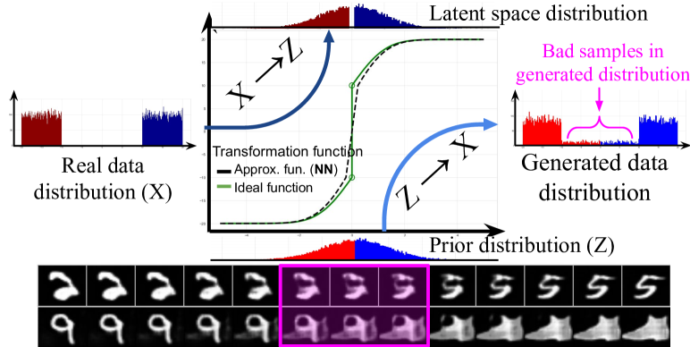
Figure 1: Illustration of an ideal mapping (green plot, a non-invertible mapping of a disconnected uniform distribution to a uni-modal Gaussian), and its invertible approximation (dotted plot) learned by a neural network. The approximate mapping ($X\rightarrow Z$) introduces a discontinuity in the latent-space (top), whose inverse ($Z\rightarrow X$) when used for generation from a uni-modal prior (bottom) reveals implausible samples (in purple).

Despite the success of GAN, the potential of such a framework has certain limitations. GAN is trained to look for the best possible approximate $P_{g}(X)$ of the target data distribution $P_{d}(X)$ within the boundaries restricted by the choice of latent variable setting (i.e. the dimension of latent embedding and the type of prior distribution) and the computational capacity of the generator network (characterized by its architecture and parameter size). Such a limitation is more prominent in the presence of highly diverse intra-class and inter-class variations, where the given target data spans a highly sparse non-linear manifold. This indicates that the underlying data distribution $P_{d}(X)$ would constitute multiple, sparsely spread, low-density regions. Considering enough capacity of the generator architecture (Universal Approximation Theorem [19]), GAN guarantees convergence to the true data distribution. However, the validity of the theorem does not hold for mapping functions involving discontinuities (Fig. 1), as exhibited by natural image or text datasets. Furthermore, various regularizations [7, 32] imposed in the training objective inevitably restrict the generator to exploit its full computational potential.

A reasonable solution to address the above limitations could be to realize multi-modal prior in place of the single-mode distribution in the general GAN framework. Several recent approaches explored this direction by explicitly enforcing the generator to capture diverse multi-modal target distribution [15, 21]. The prime challenge encountered by such approaches is attributed to the choice of the number of modes to be considered for a given set of fully-unlabelled data samples. To better analyze the challenging scenario, let us consider an extreme case, where a very high number of modes is chosen in the beginning without any knowledge of the inherent number of categories present in a dataset. In such a case, the corresponding generative model would deliver a higher inception score [4] as a result of dedicated prior modes for individual sub-categories or even sample level hierarchy. This is a clear manifestation of “overfitting in generative modeling” as such a model would generate reduced or a negligible amount of novel samples as compared to a single-mode GAN. Intuitively, the ability to interpolate between two samples in the latent embedding space [38, 30] demonstrates continuity and generalizability of a generative model. However, such an interpolation is possible only within a pair of samples belonging to the same mode specifically in the case of multi-modal latent distribution. It reveals a clear trade-off between the two schools of thoughts, that is, multi-modal latent distribution has the potential to model a better estimate of $P_{d}(X)$ as compared to a single-mode counterpart, but at a cost of reduced generalizability depending on the choice of mode selection. This also highlights the inherent trade-off between quality (multi-modal GAN) and diversity (single-mode GAN) of a generative model [29] specifically in the absence of a concrete definition of natural data distribution.

An ideal generative framework addressing the above concerns must have the following important traits:

• The framework should allow enough flexibility in the design choice of the number of modes to be considered for the latent variable distribution.

• Flexibility in generation of novel samples depending on varied preferences of quality versus diversity according to the intended application in focus (such as unsupervised clustering, hierarchical classification, nearest neighbor retrieval, etc.).

• Flexibility to adapt to a similar but different class of additional data samples introduced later in absence of the initial data samples (incremental learning setting).

In this work, we propose a novel generative modeling framework, which is flexible enough to address the quality-diversity trade-off in a given multi-modal data distribution. We introduce GAN-Tree, a hierarchical generative modeling framework consisting of multiple GANs organized in a specific order similar to a binary-tree structure. In contrast to the bottom-up approach incorporated by recent multi-modal GAN [35, 21, 15], we follow a top-down hierarchical divisive clustering procedure. First, the root node of the GAN-Tree is trained using a single-mode latent distribution on the full target set aiming maximum level of generalizability. Following this, an unsupervised splitting algorithm is incorporated to cluster the target set samples accessed by the parent node into two different clusters based on the most discriminative semantic feature difference. After obtaining a clear cluster of target samples, a bi-modal generative training procedure is realized to enable the generation of plausible novel samples from the predefined children latent distributions. To demonstrate the flexibility of GAN-Tree, we define GAN-Set, a set of mutually exclusive and exhaustive tree-nodes which can be utilized together with the corresponding prior distribution to generate samples with the desired level of quality vs diversity. Note that the leaf nodes would realize improved quality with reduced diversity whereas the nodes closer to the root would yield a reciprocal effect.

The hierarchical top-down framework opens up interesting future upgradation possibilities, which is highly challenging to realize in general GAN settings. One of them being incremental GAN-Tree, denoted as iGAN-Tree. It supports incremental generative modeling in a much efficient manner, as only a certain branch of the full GAN-Tree has to be updated to effectively model distribution of a new input set. Additionally, the top-down setup results in an unsupervised clustering of the underlying class-labels as a byproduct, which can be further utilized to develop a classification model with implicit hierarchical categorization.

2 Related work

Commonly, most of the generative approaches realize the data distribution as a mapping from a predefined prior distribution [14]. BEGAN [5] proposed an autoencoder based GAN, which adversarially minimizes an energy function [37] derived from Wasserstein distance [2]. Later, several deficiencies in this approach have been explored, such as mode-collapse [33], unstable generator convergence [26, 1], etc. Recently, several approaches propose to use an inference network [7, 24], $E:\mathcal{X}\rightarrow\mathcal{Z}$, or minimize the joint distribution $P(\mathcal{X},\mathcal{Z})$ [10, 12] to regularize the generator from mode-collapse. Although these approaches effectively address mode-collapse, they suffer from the limitations of modeling disconnected multi-modal data [21], using single-mode prior and the capacity of single generator transformation as discussed in Section 1.

To effectively address multi-modal data, two different approaches have been explored in recent works viz. a) multi-generator model and b) single generator with multi-mode prior. Works such as [13, 18, 21] propose to utilize multiple generators to account for the discontinuous multi-modal natural distribution. These approaches use a mode-classifier network either separately [18] or embedded with a discriminator [13] to enforce learning of mutually exclusive and exhaustive data modes dedicated to individual generator network. Chen et al. [8] proposed Info-GAN, which aims to exploit the semantic latent source of variations by maximizing the mutual information between the generated image and the latent code. Gurumurthy et al. [15] proposed to utilize a Gaussian mixture prior with a fixed number of components in a single generator network. These approaches used a fixed number of Gaussian components and hence do not offer much flexibility on the scale of quality versus diversity required by the end task in focus. Inspired by boosting algorithms, AdaGAN [35] proposes an iterative procedure, which incrementally addresses uncovered data modes by introducing new GAN components using the sample re-weighting technique.

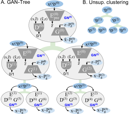
Figure 2: Illustration of the hierarchical structure of GAN-Tree (part A) and unsupervised clustering of data samples $\mathcal{D}$ in a hierarchical fashion (part B). Composition of a single GN at the root level shows how the networks are used in an ALI [12] framework inside a GNode.

3 Approach

In this section, we provide a detailed outline of the construction scheme and training algorithm of GAN-Tree (Section 3.1-3.3). Further, we discuss the inference methods for fetching a GAN-Set from a trained GAN-Tree for generation (Section 3.4). We also elaborate on the procedure to incrementally extend a previously trained GAN-Tree using new data samples from a different category (Section 3.5).

3.1 Formalization of GAN-Tree

A GAN-Tree is a full binary tree where each node indexed with $i$, GN⁽ⁱ⁾ (GNode), represents an individual GAN framework. The root node is represented as GN⁽⁰⁾ with the corresponding children nodes as GN⁽¹⁾ and GN⁽²⁾ (see Fig. 2). Here we give a brief overview of a general GAN-Tree framework. Given a set of target samples $\mathcal{D}$ = $(x_{i})^{n}_{i=1}$ drawn from a true data distribution $\mathcal{P}_{d}$, the objective is to optimize the parameters of the mapping $G:\mathcal{Z}\rightarrow\mathcal{X}$, such that the distribution of generated samples $G(z)\sim\mathcal{P}_{g}$ approximates the target distribution $\mathcal{P}_{d}$ upon randomly drawn latent vectors $z\sim\mathcal{P}_{z}$. Recent generative approaches [7] propose to simultaneously train an inference mapping, $E:\mathcal{X}\rightarrow\mathcal{Z}$ to avoid mode-collapse. In this paper, we have used Adversarially Learned Inference (ALI) [12] framework as the basic GAN formulation for each node of GAN-Tree. However, one can employ any other GAN framework for training the individual GAN-Tree nodes, if it satisfies the specific requirement of having an inference mapping.

Algorithm 1 GAN-Tree Construction/Training Algorithm

1:input: GAN-Tree tree

2:node $\leftarrow$ createRoot(tree)

3:Train $E^{(0)}_{pre}$, $G^{(0)}$ and $D^{(0)}$ with GAN Training procedure with Unimodal prior $\mathcal{P}^{(0)}_{z}$ = $\mathcal{N}(0,\mathcal{I})$

4:while CanFurtherSplit(tree) do

5:    $\mathrm{S}\leftarrow$ LeafNodes(tree)

6:    $i\leftarrow\operatorname*{argmin}_{j\in\mathrm{S}}$ $\dfrac{1}{|\mathcal{D}^{(j)}|}\sum_{x\in\mathcal{D}^{(j)}}{p}_{g}^{(j)}(x)$

7:    Initialize $E^{(i)}$ with params of $E^{(par(i))}$

8:    Initialize $G^{(l)}$ and $G^{(r)}$ with params of $G^{(i)}$

9:    Initialize $D^{(l)}$ and $D^{(r)}$ with params of $D^{(i)}$

10:    $\mathcal{P}^{(l)}_{z}\leftarrow\mathcal{N}(\dfrac{k\sigma}{2\sqrt{d}}\mathbf{1},\mathcal{I})$, $\mathcal{P}^{(r)}_{z}\leftarrow\mathcal{N}(-\dfrac{k\sigma}{2\sqrt{d}}\mathbf{1},\mathcal{I})$

11:    ModeSplitProcedure (GN⁽ⁱ⁾)

12:    $\pi^{(l)}\leftarrow\dfrac{|\mathcal{D}^{(l)}|}{|\mathcal{D}^{(i)}|}$, $\pi^{(r)}\leftarrow\dfrac{|\mathcal{D}^{(r)}|}{|\mathcal{D}^{(i)}|}$

13:    BiModalGAN-Training(GN⁽ⁱ⁾)

Root node ($GN^{(0)}$). Assuming $\mathcal{D}^{(0)}$ as the set of complete target samples, the root node $GN^{(0)}$ is first trained using a single-mode latent prior distribution $z\sim\mathcal{P}^{(0)}_{z}$. As shown in Fig. 2; $E^{(0)}_{pre}$, $G^{(0)}$ and $D^{(0)}$ are the encoder, generator and discriminator network respectively for the root node with index-$0$; which are trained to generate samples, $x\sim\mathcal{P}_{g}^{(0)}$ approximating $\mathcal{P}_{d}^{(0)}$. Here, $\mathcal{P}_{d}^{(0)}$ is the true target distribution whose samples are given as $x\in\mathcal{D}^{(0)}$. After obtaining the best approximate $\mathcal{P}_{g}^{(0)}$, the next objective is to improve the approximation by considering the multi-modal latent distribution in the succeeding hierarchy of GAN-Tree.

Children nodes ($GN^{(l)}$ and $GN^{(r)}$). Without any choice of the initial number of modes, we plan to split each GNode into two children nodes (see Fig. 2). In a general setting, assuming $p$ as the parent node index with the corresponding two children nodes indexed as $l$ and $r$, we define $l=left(p)$, $r=right(p)$, $p=par(l)$ and $p=par(r)$ for simplifying further discussions. Considering the example shown in Fig. 2, with the parent index $p=0$, the indices of left and right child would be $l=1$ and $r=2$ respectively. A novel binary Mode-splitting procedure (Section 3.2) is incorporated, which, without using the label information, effectively exploits the most discriminative semantic difference at the latent $\mathcal{Z}$ space to realize a clear binary clustering of the input target samples. We obtain cluster-set $\mathcal{D}^{(l)}$ and $\mathcal{D}^{(r)}$ by applying Mode-splitting on the parent-set $\mathcal{D}^{(p)}$ such that $\mathcal{D}^{(p)}=\mathcal{D}^{(l)}\cup\mathcal{D}^{(r)}$. Note that, a single encoder $E^{(p)}$ network is shared by both the child nodes $GN^{(l)}$ and $GN^{(r)}$ as it is also utilized as a routing network, which can route a given target sample $x$ from the root-node to one of the leaf-nodes by traversing through different levels of the full GAN-Tree. The bi-modal latent distribution at the output of the common encoder $E^{(p)}$ is defined as $z\sim\mathcal{P}_{z}^{(l)}$ and $z\sim\mathcal{P}_{z}^{(r)}$for the left and right child-node respectively.

After the simultaneous training of $GN^{(l)}$ and $GN^{(r)}$ using a Bi-Modal Generative Adversarial Training (BiMGAT) procedure (Section 3.3), we obtain an improved approximation ($\mathcal{P}_{g}^{(p)}$) of the true distribution ($\mathcal{P}_{d}^{(p)}$) as $\mathcal{P}_{g}^{(p)}=\pi^{(l)}\mathcal{P}_{g}^{(l)}+\pi^{(r)}\mathcal{P}_{g}^{(r)}$. Here, the generated distributions $\mathcal{P}_{g}^{(l)}$ and $\mathcal{P}_{g}^{(r)}$ are modelled as $G^{(l)}(z\sim\mathcal{P}_{z}^{(l)})$ and $G^{(r)}(z\sim\mathcal{P}_{z}^{(r)})$ respectively (Algo. 1). Similarly, one can split the tree further to effectively capture the inherent number of modes associated with the true data distribution $\mathcal{P}_{d}$.

Node Selection for split and stopping-criteria. A natural question then arises of how to decide which node to split first out of all the leaf nodes present at a certain state of GAN-Tree? For making this decision, we choose the leaf node which gives minimum mean likelihood over the data samples labeled for it (lines 5-6, Algo. 1). Also, the stopping criteria on the splitting of GAN-Tree has to be defined carefully to avoid overfitting to the given target data samples. For this, we make use of a robust IRC-based stopping criteria [16] over the embedding space $\mathcal{Z}$, preferred against standard AIC and BIC metrics. However, one may use a fixed number of modes as a stopping criteria and extend the training from that point as and when required.

Algorithm 2 Mode Split Procedure

1:input: GN with index $i$, left and right child $l$ and $r$

2:Initialize unassigned bag $\mathcal{B}_{u}$ with $\mathcal{D}^{(i)}$, assigned bag $\mathcal{B}_{a}$ with $\phi$, and cluster label map $\mathrm{L}$ with $\phi$

3:while  $|\mathcal{B}_{u}|\neq 0$ do

4:    for $n_{0}$ iterations do

5:         Sample minibatch $x_{u}$ of $m$ data samples

6:           {$x^{(1)}_{u},x^{(2)}_{u},...,x^{(m)}_{u}$} from $\mathcal{B}_{u}$.

7:         Sample minibatch $x_{a}$ of $m$ data samples

8:           {$x^{(1)}_{a},x^{(2)}_{a},...,x^{(m)}_{a}$} from $\mathcal{B}_{a}$.

9:         for $j$ from $1$ to $m$ do

10:             $z^{(j)}_{a}\leftarrow E^{(i)}(x^{(j)}_{a})$;   $z^{(j)}_{u}\leftarrow E^{(i)}(x^{(j)}_{u})$

11:             ${c}_{j}=\mathrm{L}(x^{(j)}_{a})$ (assigned cluster label)

12:             $t_{j}=\operatorname*{argmax}_{k\in\{l,r\}}p(k|z^{(j)}_{u})$ (temp. label)          

13:         $\mathcal{L}_{recon}^{(a)}\leftarrow\frac{1}{m}\sum_{j=1}^{m}\left\lVert x^{(j)}_{a}-G^{(c_{j})}(z^{(j)}_{a})\right\rVert^{2}_{2}$

14:         $\mathcal{L}_{recon}^{(u)}\leftarrow\frac{1}{m}\sum_{j=1}^{m}\left\lVert x^{(j)}_{u}-G^{(t_{j})}(z^{(j)}_{u})\right\rVert^{2}_{2}$

15:         $\mathcal{L}_{nll}^{(a)}\leftarrow\frac{1}{m}\sum_{j=1}^{m}-log(p^{(c_{j})}_{z}(z^{(j)}_{a}))$

16:         $\mathcal{L}_{nll}^{(u)}\leftarrow\frac{1}{m}\sum_{j=1}^{m}-log(p^{(t_{j})}_{z}(z^{(j)}_{u}))$

17:         $\mathcal{L}_{split}\leftarrow\mathcal{L}_{recon}^{(a)}+\mathcal{L}_{recon}^{(u)}+\mathcal{L}_{nll}^{(a)}+\mathcal{L}_{nll}^{(u)}$

18:         Update parameters $\Theta_{E^{(i)}}$, $\Theta_{G^{(l)}}$, $\Theta_{G^{(r)}}$

19:           by optimizing $\mathcal{L}_{split}$ using Adam     

20:    for $x\in\mathcal{B}_{u}$ do

21:         if $\max_{k\in\{l,r\}}p^{(k)}_{z}(E^{(i)}(x))>\gamma_{0}$ then

22:             Move $x$ from $\mathcal{B}_{u}$ to $\mathcal{B}_{a}$

23:             $\mathrm{L}(x)\leftarrow\operatorname*{argmax}_{k\in\{l,r\}}p(k|E^{(i)}(x))$              

3.2 Mode-Split procedure

The mode-split algorithm is treated as a basis of the top-down divisive clustering idea, which is incorporated to construct the hierarchical GAN-Tree by performing binary split of individual GAN-Tree nodes. The splitting algorithm must be efficient enough to successfully exploit the highly discriminative semantic characteristics in a fully-unsupervised manner. To realize this, we first define $P_{z}^{(l)}=\mathcal{N}(\mu^{(l)},\Sigma^{(l)})$ and $P_{z}^{(r)}=\mathcal{N}(\mu^{(r)},\Sigma^{(r)})$ as the fixed normal prior distributions (non-trainable) for the left and right children respectively. A clear separation between these two priors is achieved by setting the distance between the mean vectors as $k\sigma$ with $\Sigma^{(l)}=\Sigma^{(r)}=\sigma^{2}\mathcal{I}_{d}$; where $\mathcal{I}_{d}$ is a $d\times d$ identity matrix. Assuming $i$ as the parent node index, $\mathcal{D}^{(i)}$ is the cluster of target samples modeled by $GN^{(i)}$. Put differently, the objective of the mode-split algorithm is to form two mutually exclusive and exhaustive target data clusters $\mathcal{D}^{(l)}$ and $\mathcal{D}^{(r)}$, by utilizing the likelihood of the latent representations to the predefined priors $P_{z}^{(l)}$ and $P_{z}^{(r)}$.

To effectively realize mode-splitting (Algo. 2), we define two different bags; a) assigned bag $\mathcal{B}_{a}$ and b) unassigned bag $\mathcal{B}_{u}$. $\mathcal{B}_{a}$ holds the semantic characteristics of individual modes in the form of representative high confidence labeled target samples. Here, the assigned labeled samples are a subset of the parent target samples, $x\in\mathcal{D}^{(i)}$, with the corresponding hard assigned cluster-id obtained using the likelihood to the predefined priors (line 11, Algo. 2) in the transformed encoded space. We refer it as a hard-assignment as we do not update the cluster label of these samples once they are moved from $\mathcal{B}_{u}$ to the assigned bag, $\mathcal{B}_{a}$. This effectively tackles mode-collapse in the later iterations of the mode-spilt procedure. For the samples in $\mathcal{B}_{u}$, a temporary cluster label is assigned depending on the prior with maximum likelihood (line 12, Algo. 2) to aggressively move them towards one of the binary modes (lines 19-22, Algo. 2). Finally, the algorithm converges when all the samples in $\mathcal{B}_{u}$ are moved to $\mathcal{B}_{a}$. The algorithm involves simultaneous update of three different network parameters (line 18, Algo. 2) using a final loss function $\mathcal{L}_{split}$ consisting of:

• the likelihood maximization term $\mathcal{L}_{nll}$ for samples in both $\mathcal{B}_{a}$ and $\mathcal{B}_{u}$ (lines 15-16) encouraging exploitation of a binary discriminative semantic characteristic, and

• the semantic preserving reconstruction loss $\mathcal{L}_{recon}$ computed using the corresponding generator i.e. $G^{(l)}$ and $G^{(r)}$ (lines 13-14). This is used as a regularization to hold the semantic uniqueness of the individual samples avoiding mode-collapse.

3.3 BiModal Generative Adversarial Training

The mode-split algorithm does not ensure matching of the generated distribution $G^{(l)}(z\sim\mathcal{P}_{z}^{(l)})$ and $G^{(r)}(z\sim\mathcal{P}_{z}^{(r)})$ with the expected target distribution $\mathcal{P}_{d}^{(l)}$ and $\mathcal{P}_{d}^{(r)}$ without explicit attention. Therefore to enable generation of plausible samples from the randomly drawn prior latent vectors, a generative adversarial framework is incorporated simultaneously for both left and right children. In ALI [12] setting, the loss function involves optimization of the common encoder along with both the generators in an adversarial fashion; utilizing two separate discriminators, which are trained to distinguish $E^{(p)}(x\in\mathcal{D}^{(l)})$ and $E^{(p)}(x\in\mathcal{D}^{(r)})$ from $z\sim\mathcal{P}_{z}^{(l)}$ and $z\sim\mathcal{P}_{z}^{(r)}$ respectively.

3.4 GAN-Set: Generation and Inference

To utilize a generative model spanning the entire data distribution $\mathcal{P}_{d}$, an end-user can select any combination of nodes from a fully trained GAN-Tree (i.e. GAN-Set) such that the data distribution they model is exhaustive and mutually exclusive. However, to generate only a subset of the full data distribution, one may choose a mutually exclusive, but non-exhaustive set - Partial GAN-Set.

For a use case where extreme preference is given to diversity in terms of the number of novel samples over quality of the generated samples, selecting a singleton set - {root} would be an apt choice. However, in a contrasting use case, one may select all the leaf nodes as a Terminal GAN-Set to have the best quality in the generated samples, albeit losing the novelty in generated samples. The most practical tasks will involve use cases where a GAN-Set is constructed as a combination of both intermediate nodes and leaf nodes.

A GAN-Set can also be used to perform clustering and label assignment for new data samples in a fully unsupervised setting. We provide a formal procedure AssignLabel in the supplementary document for performing the clustering of the data samples using a GAN-Tree.

How does GAN-Tree differ from previous works?

AdaGAN - Sequential learning approach adopted by [35] requires a fully-trained model on the previously addressed mode before addressing the subsequent undiscovered samples. As it does not enforce any constraints on the amount of data to be modeled by a single generator network, it mostly converges to more number of modes than that actually present in the data. In contrast, GAN-Tree models a mutually exclusive and exhaustive set at each splitting of a parent node by simultaneously training child generator networks. Another major disadvantage of AdaGAN is that it highly focuses on quality rather than diversity (caused by the over-mode division), which inevitably restricts the latent space interpolation ability of the final generative model.

DMGAN - Khayatkhoei et al. [21] proposed a disconnected manifold learning generative model using a multi-generator approach. They proposed to start with an overestimate of the initial number of mode components, $n_{g}$, than the actual number of modes in the data distribution $n_{r}$. As discussed before, we do not consider the existence of a definite value for the number of actual modes $n_{r}$ as considered by DMGAN, especially for diverse natural image datasets like CIFAR and ImageNet. In a practical scenario, one can not decide the initial value of $n_{g}$ without any clue on the number of classes present in the dataset. DMGAN will fail for cases where $n_{g}<n_{r}$ as discussed by the authors. Also note that unlike GAN-Tree, DMGAN is not suitable for incremental future expansion. This clearly demonstrates the superior flexibility of GAN-Tree against DMGAN as a result of the adopted top-down divisive strategy.

Algorithm 3 Incremental Node Training

1:input: Node Index $c$, New Data Sample set $\mathcal{D}^{\prime}$

2:gset = CreateTerminalGanSet(GN ^par(c))

3:Populate an empty bag $\mathcal{B}_{a}$ of assigned samples with all samples from $\mathcal{D}^{\prime}$

4:Generate $|\mathcal{D}^{\prime}|\cdot|$gset$|$ samples from $\mathcal{P}^{(gset)}_{g}$ and add them to $\mathcal{B}_{a}$; assign cluster labels based on the corresponding ancestor among the child nodes of GN ^par(c) to $\mathrm{L}$

5:Run Mode Split Procedure on GN ^(par(c)) training only $E^{(par(c))}$ and $G^{(c)}$ over samples from $\mathcal{B}_{a}$

6:Run BiModalGAN-Training over GN^(par(c)) training only $E^{(par(c))}$, $G^{(c)}$ and $D^{(c)}$

7:Re-evaluate $\pi^{(left(par(c)))}$ and $\pi^{(right(par(c)))}$

3.5 Incremental GAN-Tree: iGANTree

We advance the idea of GAN-Tree to iGAN-Tree, wherein we propose a novel mechanism to extend an already trained GAN-Tree $\mathcal{T}$ to also model samples from a set $\mathcal{D}^{\prime}$ of new data samples. An outline of the entire procedure is provided across Algorithms 3 and 4. To understand the mechanism, we start with the following assumptions from the algorithm. On termination of this procedure over $\mathcal{T}$, we expect to have a single leaf node which solely models the distribution of samples from $\mathcal{D}^{\prime}$; and other intermediate nodes which are the ancestors of this new node, should model a mixture distribution which also includes samples from $\mathcal{D}^{\prime}$.

Algorithm 4 Incremental GAN-Tree Training

1:input: GAN-Tree $T$, New Data Sample set $\mathcal{D}^{\prime}$

2:$i\leftarrow$ index(root($T$))

3:while $i$ is NOT a leaf node do

4:    $l\leftarrow$ left($i$); $r\leftarrow$ right($i$)

5:    if Avg($p_{x}^{(l)}$($\mathcal{D}^{\prime}$)) $\geq p_{z}^{(l)}({\mu}^{(l)}+d_{\sigma_{0}})$ then $i\leftarrow l$

6:    else if Avg($p_{x}^{(r)}$($\mathcal{D}^{\prime}$)) $\geq p_{z}^{(r)}({\mu}^{(r)}+d_{\sigma_{0}})$ then $i\leftarrow r$

7:    else  break     

8:Here, $i$ is the current node index

9:$j\leftarrow$ NewId() (new parent index)

10:$k\leftarrow$ NewId() (new child index)

11:par($k$) $\leftarrow j$;  par($j$) $\leftarrow$ par($i$);  par($i$) $\leftarrow j$

12:if $i$ = index(root($T$)) then

13:    root($T$) $\leftarrow j$;  left($j$) $\leftarrow i$;  right($j$) $\leftarrow k$

14:else if $i$ was the left child of its previous parent then

15:    left(par($j$)) $\leftarrow j$;  left($j$) $\leftarrow i$;  right($j$) $\leftarrow k$

16:else

17:    right(par($j$)) $\leftarrow j$;   left($j$) $\leftarrow k$;   right($j$) $\leftarrow i$

18:Create networks $G^{(k)}$, $D^{(k)}$ with random initialization

19:Train $E^{(j)},G^{(k)}$ and $D^{(k)}$ with $\mathcal{L}_{recon}$ and $\mathcal{L}_{adv}$

20:$E^{(par(j))}\leftarrow$ copy($E^{(par(i))}$)

21:$G^{(j)}\leftarrow$ copy($G^{(i)}$); $D^{(j)}\leftarrow$ copy($D^{(i)}$); $i\leftarrow$ par($i$)

22:while GN⁽ⁱ⁾ is not root($T$) do

23:    IncrementalNodeTrain($i$); $i\leftarrow$ par($i$) end while

24:Train GN⁽ⁱ⁾ with GAN Training Procedure on $\mathcal{D}$’ and generated samples from Terminal GAN-Set.

To achieve this, we first find out the right level of hierarchy and position to insert this new leaf node using a seek procedure (lines 2-8 in Algo. 4). Here $p_{x}^{(l)}(x)=p_{z}^{(l)}(E^{(l)}(x))$ and similarly for $r$, in lines 5-6. Let’s say the seek procedure stops at node index $i$. We now introduce 2 new nodes GN^(j) and GN^(k) in the tree and perform reassignment (lines 11-17 in Algo. 4). The new child node GN^(k) models only the new data samples; and the new parent node GN^(j) models a mixture of $\mathcal{P}^{(i)}_{g}$ and $\mathcal{P}^{(k)}_{g}$. This brings us to the question, how do we learn the new distribution modeled by GN^(par(i)) and its ancestors? To solve this, we follow a bottom-up training approach from GN^(par(i)) to GN^(root(T)), incrementally training each node on the branch with samples from $\mathcal{D}$’ to maintain the hierarchical property of the GAN-Tree (lines 22-24, Algo. 4).

Now, the problem reduces down to retraining the parent $E^{(p)}$ and the child $G^{(c)}$ and $D^{(c)}$ networks at each node in the selected branch, such that (i) $E^{(p)}$ correctly routes the generated data samples $x$ to the proper child node and (ii) the samples from $\mathcal{D}^{\prime}$ are modeled by the new distribution $\mathcal{P}^{\prime}_{g}$ at all the ancestor nodes of GN^(k), remembering the samples from distribution $\mathcal{P}_{g}$ at the same time. Moreover, we make no assumption of having the data samples $\mathcal{D}$ on which the GAN-Tree was trained previously. To solve the problem of training the node GN${}^{(i^{\prime})}$, we make use of terminal GAN-Set of the sub GAN-Tree rooted at GN${}^{(i^{\prime})}$ to generate samples for retraining the node. A thorough procedure of how each node is trained incrementally is illustrated in Algo. 3. Also, note that we use the mean likelihood measure to decide which of the two child nodes has the potential to model the new samples. We select the child whose mean vector has the minimum average Mahalanobis distance ($d_{\sigma}$) from the embeddings of the samples of $\mathcal{D}$’. This idea can also be implemented to have a full persistency over the structure [11] (further details in Supplementary).

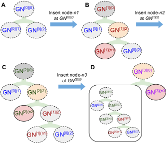
Figure 3: Snapshots of the different versions of incrementally obtained GAN-Tree. Here A is the pretrained GAN-Tree over which Algo. 4 is run to obtain B, and subsequently C and D. Each transition highlights the branch which is updated in gray, with the new child node in red, the new parent node in orange, while the rest of the nodes stay intact. In B, nodes labeled with red are the ones which are updated. Similarly, in C and D, the updated nodes are labeled with green and purple respectively. It is illustrated that just by incrementally adding a new branch by updating nodes from its previous version, it exploits the full persistence of the GAN-Tree and provides all the versions of root nodes - GN^[0:4](0).

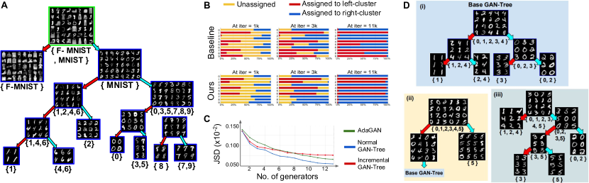
Figure 4: Part A: Illustration of the GAN-Tree training procedure over MNIST+Fashion-MNIST dataset. Part B: Effectiveness of our mode-split procedure (with bagging) against the baseline deep-clustering technique (without bagging) on MNIST root node. Our approach divides the digits into two groups in a much cleaner way (at iter=11k). Part C: We evaluate the GAN-Tree and iGAN-Tree algorithms against the prior incremental training method AdaGAN [35]. We train up to 13 generators and evaluate their mean JS Divergence score (taken over 5 repetitions). Part D: Incremental GAN-Tree training procedure (i) Base GAN-Tree, trained over digits 0-4 (ii) GAN-Tree after addition of digit 5, with $d_{\sigma_{0}}$ = 4 (iii) GAN-Tree after addition of digit 5, with $d_{\sigma_{0}}$ = 9.

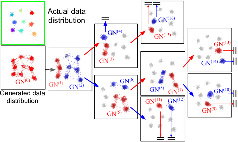
Figure 5: Illustration of the GAN-Tree progression over the toy dataset.

4 Experiments

In this section, we discuss a thorough evaluation of GAN-Tree against baselines and prior approaches. We decide not to use any improved learning techniques (as proposed by SNGAN [27] and SAGAN [36]) for the proposed GAN-Tree framework to have a fair comparison against the prior art [21, 13, 18] targeting multi-modal distribution.

GAN-Tree is a multi-generator framework, which can work on a multitude of basic GAN formalizations (like AAE [25], ALI [12], RFGAN [3] etc.) at the individual node level. However, in most of the experiments we use ALI [12] except for CIFAR, where both ALI [12] and RFGAN [3] are used to demonstrate generalizability of GAN-Tree over varied GAN formalizations. Also note that we freeze parameter update of lower layers of encoder and discriminator; and higher layers of the generator (close to data generation layer) in a systematic fashion, as we go deeper in the GAN-Tree hierarchical separation pipeline. Such a parameter sharing strategy helps us to remove overfitting at an individual node level close to the terminal leaf-nodes.

We employ modifications to the commonly used DCGAN [30] architecture for generator, discriminator and encoder networks while working on image datasets i.e. MNIST (32$\times 32$), CIFAR-10 (32$\times 32$) and Face-Bed (64$\times 64$)). However, unlike in DCGAN, we use batch normalization [20] with Leaky ReLU non-linearity inline with the prior multi-generator works [18]. While training GAN-Tree on Imagenet [31], we follow the generator architecture used by SNGAN [27] for a generation resolution of 128$\times$128 with RFGAN [3] formalization. For both mode-split and BiModal-GAN training we employ Adam optimizer [22] with a learning rate of 0.001.

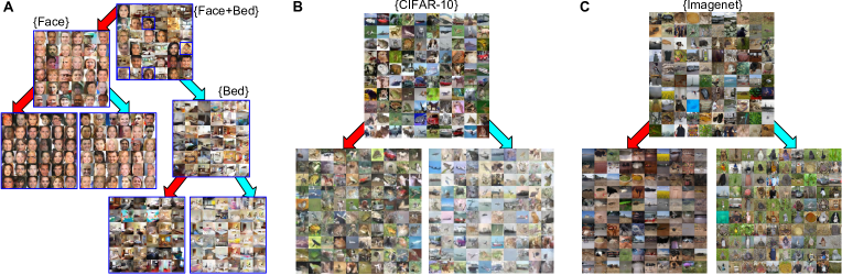
Figure 6: Generation results on RGB image datasets A: FaceBed, B: CIFAR-10, C: ImageNet. The root node generations of FaceBed show a few implausible generations, which are reduced with further splits. The left child of the root node generates faces, while the right child generates beds. Further splitting the face node, we see that one child node generates images with darker background or darker hair colour, while the other generates images with lighter background or lighter hair colour. Similar trends are observed in the splits of Bed Node in Part A, and also in child nodes of CIFAR-10 and ImageNet.

Effectiveness of the proposed mode-split algorithm. To verify the effectiveness of the proposed mode-split algorithm, we perform an ablation analysis against a baseline deep-clustering [34] technique on the 10-class MNIST dataset. Performance of GAN-Tree highly depends on the initial binary split performed at the root node, as an error in cluster assignment at this stage may lead to multiple-modes for a single image category across both the child tree hierarchy. Fig. 4B clearly shows the superiority of mode-split procedure when applied at the MNIST root node.

Table 1: Comparison of inter-class variation (JSD) for MNIST ($\times 10^{-2}$) and Face-Bed ($\times 10^{-4}$); and FID score on Face-Bed inline with [21].

Model	#Gen	JSD MNIST	JSD Face-Bed	FID Face-Bed
DMWGAN [21]	20	$0.21\pm 0.05$	$0.42\pm 0.23$	$7.58\pm 0.10$
DMWGAN-PL [21]	20	$0.08\pm 0.03$	$0.11\pm 0.06$	$7.30\pm 0.12$
Ours GAN-Set	5	$0.08\pm 0.02$	$0.10\pm 0.06$	$7.20\pm 0.11$
Ours GAN-Set	10	$0.06\pm 0.02$	$0.09\pm 0.04$	$7.00\pm 0.10$

Evaluation on Toy dataset. We construct a synthetic dataset by sampling 2D points from a mixture of nine disconnected Gaussian distributions with distinct means and covariance parameters. The complete GAN-Tree training procedure over this dataset is illustrated in Fig. 5. As observed, the distribution modeled at each pair of child nodes validates the mutually exclusive and exhaustive nature of child nodes for the corresponding parent.

Evaluation on MNIST. We show an extensive comparison of GAN-Tree against DMWGAN-PL [21] across various qualitative metrics on MNIST dataset. Table 1 shows the quantitative comparison of inter-class variation against previous state-of-the-art approaches. It highlights the superiority of the proposed GAN-Tree framework.

Evaluation on compositional-MNIST. As proposed by Che et al. [7], the compositional-MNIST dataset consists of 3 random digits at 3 different quadrants of a full 64$\times$64 resolution template, resulting in a data distribution of 1000 unique modes. Following this, a pre-trained MNIST classifier is used for recognizing digits from the generated samples, to compute the number of modes covered while generating from all of the 1000 variants. Table 2 highlights the superiority of GAN-Tree against MAD-GAN [13].

iGAN-Tree on MNIST. We show a qualitative analysis of the generations of a trained GAN-Tree after incrementally adding data samples under different settings. We first train a GAN-Tree for 5 modes on MNIST digits 0-4. We then train it incrementally with samples of the digit 5 and show how the modified structure of the GAN-Tree looks like. Fig. 4D shows a detailed illustration for this experiment.

GAN-Tree on MNIST+F-MNIST and Face-Bed. We perform the divisive GAN-Tree training procedure on two mixed datasets. For MNIST+Fashion-MNIST, we combine 20K images from both the datasets individually. Similarly, following [21], we combine Face-Bed to demonstrate the effectiveness of GAN-Tree to model diverse multi-modal data supported on a disconnected manifold (as highlighted by Table 1). The hierarchical generations for MNIST+F-MNIST and the mixed Face-Bed datasets are shown in Fig. 4A and Fig. 6A respectively.

Table 2: Comparison of GAN-Tree against state-of-the-art GAN approaches on compositional-MNIST dataset inline with [13].

Methods	KL Div.$\downarrow$	Modes covered $\uparrow$
WGAN [1]	0.25	1000
MAD-GAN [13]	0.074	1000
GAN-Set (root)	0.16	980
GAN-Set (5 G-Nodes)	0.10	1000
GAN-Set (10 G-Nodes)	0.072	1000

On CIFAR-10 and ImageNet. In Table 3, we report the inception score [32] and FID [17] obtained by GAN-Tree against prior works on both CIFAR-10 and ImageNet dataset. We separately implement the prior multi-modal approaches, a) GMVAE [9] b) ClusterGAN [28], and also the prior multi-generator works, a) MADGAN [13] b) DMWGAN-PL [21] with a fixed number of generators. Additionally, to demonstrate the generalizability of the proposed framework with varied GAN formalizations at the individual node-level, we implement GAN-Tree with ALI [12], RFGAN [3], and BigGAN [6] as the basic GAN setup. Note that, we utilize the design characteristics of BigGAN without accessing the class-label information, along with RFGAN’s encoder for both CIFAR-10 and ImageNet.

In Table 3, all the approaches targeting ImageNet dataset use modified ResNet-50 architecture, where the total number of parameter varies depending on the number of generators (considering the hierarchical weight sharing strategy) as reported under the #Param column. While comparing generation performance, one needs access to a selected GAN-Set instead of the entire GAN-Tree. In Table 3, the performance of GAN-Set (RFGAN) with 3 generators (i.e. GAN-Tree with total 5 generators) is superior to DMWGAN-PL [21] and MADGAN [13], each with 10 generators. This clearly shows the superior computational efficiency of GAN-Tree against prior multi-generator works. An exemplar set of generated images with the first root node split is presented in Fig. 6B and 6C.

Table 3: Inception (IS) and FID scores on CIFAR-10 and Imagenet dataset computed on 5K with varied number of generators.

Method	#Gen	CIFAR-10		ImageNet
		IS $\uparrow$	FID $\downarrow$	IS $\uparrow$	FID $\downarrow$	#Param
GMVAE [9]	1	6.89	39.2	-	-	-
ClusterGAN [28]	1	7.02	37.1	-	-	-
RFGAN [3] (root-node)	1	6.87	38.0	20.01	46.4	50M
BigGAN (w/o label)	1	7.19	36.7	20.89	42.5	50M
MADGAN [13]	10	7.33	35.1	20.92	38.3	205M
DMWGAN-PL [21]	10	7.41	33.1	21.57	37.8	205M
Ours GAN-Set (ALI)	3	7.42	32.5	-	-	-
Ours GAN-Set (ALI)	5	7.63	28.2	-	-	-
Ours GAN-Set (RFGAN)	3	7.60	28.3	21.97	34.0	65M
Ours GAN-Set (RFGAN)	5	7.91	27.8	24.84	29.4	105M
Ours GAN-Set (BigGAN)	3	8.12	25.2	22.38	31.2	130M
Ours GAN-Set (BigGAN)	5	8.60	21.9	25.93	27.1	210M

5 Conclusion

GAN-Tree is an effective framework to address natural data distribution without any assumption on the inherent number of modes in the given data. Its hierarchical tree structure gives enough flexibility by providing GAN-Sets of varied quality-vs-diversity trade-off. This also makes GAN-Tree a suitable candidate for incremental generative modeling. Further investigation on the limitations and advantages of such a framework will be explored in the future.

Acknowledgements. This work was supported by a Wipro PhD Fellowship (Jogendra) and a grant from ISRO, India.

See pages 1-1 of suppl_gantree_noref.pdf See pages 2-2 of suppl_gantree_noref.pdf See pages 3-3 of suppl_gantree_noref.pdf See pages 4-4 of suppl_gantree_noref.pdf See pages 5-5 of suppl_gantree_noref.pdf

References

- [1] Martin Arjovsky and Léon Bottou. Towards principled methods for training generative adversarial networks. In International Conference on Learning Representations, 2017.
- [2] Martin Arjovsky, Soumith Chintala, and Léon Bottou. Wasserstein generative adversarial networks. In International Conference on Machine Learning, 2017.
- [3] Duhyeon Bang and Hyunjung Shim. High quality bidirectional generative adversarial networks. In International Conference on Machine Learning, 2018.
- [4] Shane Barratt and Rishi Sharma. A note on the inception score. arXiv preprint arXiv:1801.01973, 2018.
- [5] David Berthelot, Thomas Schumm, and Luke Metz. Began: boundary equilibrium generative adversarial networks. arXiv preprint arXiv:1703.10717, 2017.
- [6] Andrew Brock, Jeff Donahue, and Karen Simonyan. Large scale gan training for high fidelity natural image synthesis. In International Conference on Learning Representations, 2019.
- [7] Tong Che, Yanran Li, Athul Paul Jacob, Yoshua Bengio, and Wenjie Li. Mode regularized generative adversarial networks. In International Conference on Learning Representations, 2017.
- [8] Xi Chen, Yan Duan, Rein Houthooft, John Schulman, Ilya Sutskever, and Pieter Abbeel. Infogan: Interpretable representation learning by information maximizing generative adversarial nets. In Advances in neural information processing systems, 2016.
- [9] Nat Dilokthanakul, Pedro AM Mediano, Marta Garnelo, Matthew CH Lee, Hugh Salimbeni, Kai Arulkumaran, and Murray Shanahan. Deep unsupervised clustering with gaussian mixture variational autoencoders. arXiv preprint arXiv:1611.02648, 2016.
- [10] Jeff Donahue, Philipp Krähenbühl, and Trevor Darrell. Adversarial feature learning. In International Conference on Learning Representations, 2017.
- [11] James R Driscoll, Neil Sarnak, Daniel D Sleator, and Robert E Tarjan. Making data structures persistent. Journal of computer and system sciences, 38(1):86–124, 1989.
- [12] Vincent Dumoulin, Ishmael Belghazi, Ben Poole, Olivier Mastropietro, Alex Lamb, Martin Arjovsky, and Aaron Courville. Adversarially learned inference. In International Conference on Learning Representations, 2017.
- [13] Arnab Ghosh, Viveka Kulharia, Vinay Namboodiri, Philip HS Torr, and Puneet K Dokania. Multi-agent diverse generative adversarial networks. In The IEEE Conference on Computer Vision and Pattern Recognition (CVPR), 2018.
- [14] Ian Goodfellow, Jean Pouget-Abadie, Mehdi Mirza, Bing Xu, David Warde-Farley, Sherjil Ozair, Aaron Courville, and Yoshua Bengio. Generative adversarial nets. In Advances in Neural Information Processing Systems, 2014.
- [15] Swaminathan Gurumurthy, Ravi Kiran Sarvadevabhatla, and R Venkatesh Babu. Deligan: Generative adversarial networks for diverse and limited data. In The IEEE Conference on Computer Vision and Pattern Recognition (CVPR), 2017.
- [16] Kyu J Han and Shrikanth S Narayanan. A robust stopping criterion for agglomerative hierarchical clustering in a speaker diarization system. In Eighth Annual Conference of the International Speech Communication Association, 2007.
- [17] Martin Heusel, Hubert Ramsauer, Thomas Unterthiner, Bernhard Nessler, and Sepp Hochreiter. Gans trained by a two time-scale update rule converge to a local nash equilibrium. In Advances in Neural Information Processing Systems, pages 6626–6637, 2017.
- [18] Quan Hoang, Tu Dinh Nguyen, Trung Le, and Dinh Phung. Mgan: Training generative adversarial nets with multiple generators. In International Conference on Learning Representations, 2018.
- [19] Kurt Hornik, Maxwell Stinchcombe, and Halbert White. Multilayer feedforward networks are universal approximators. Neural networks, 2(5):359–366, 1989.
- [20] Sergey Ioffe and Christian Szegedy. Batch normalization: Accelerating deep network training by reducing internal covariate shift. arXiv preprint arXiv:1502.03167, 2015.
- [21] Mahyar Khayatkhoei, Maneesh Singh, and Ahmed Elgammal. Disconnected manifold learning for generative adversarial networks. arXiv preprint arXiv:1806.00880, 2018.
- [22] Diederik Kingma and Jimmy Ba. Adam: A method for stochastic optimization. arXiv preprint arXiv:1412.6980, 2014.
- [23] Diederik P Kingma and Max Welling. Auto-encoding variational bayes. arXiv preprint arXiv:1312.6114, 2013.
- [24] Anders Boesen Lindbo Larsen, Søren Kaae Sønderby, Hugo Larochelle, and Ole Winther. Autoencoding beyond pixels using a learned similarity metric. In International Conference on Machine Learning, 2016.
- [25] Alireza Makhzani, Jonathon Shlens, Navdeep Jaitly, and Ian Goodfellow. Adversarial autoencoders. In International Conference on Learning Representations, 2016.
- [26] Luke Metz, Ben Poole, David Pfau, and Jascha Sohl-Dickstein. Unrolled generative adversarial networks. arXiv preprint arXiv:1611.02163, 2016.
- [27] Takeru Miyato, Toshiki Kataoka, Masanori Koyama, and Yuichi Yoshida. Spectral normalization for generative adversarial networks. arXiv preprint arXiv:1802.05957, 2018.
- [28] Sudipto Mukherjee, Himanshu Asnani, Eugene Lin, and Sreeram Kannan. Clustergan: Latent space clustering in generative adversarial networks. In Proceedings of the AAAI Conference on Artificial Intelligence, volume 33, pages 4610–4617, 2019.
- [29] Anh Nguyen, Jeff Clune, Yoshua Bengio, Alexey Dosovitskiy, and Jason Yosinski. Plug & play generative networks: Conditional iterative generation of images in latent space. In The IEEE Conference on Computer Vision and Pattern Recognition (CVPR), 2017.
- [30] Alec Radford, Luke Metz, and Soumith Chintala. Unsupervised representation learning with deep convolutional generative adversarial networks. arXiv preprint arXiv:1511.06434, 2015.
- [31] Olga Russakovsky, Jia Deng, Hao Su, Jonathan Krause, Sanjeev Satheesh, Sean Ma, Zhiheng Huang, Andrej Karpathy, Aditya Khosla, Michael Bernstein, et al. Imagenet large scale visual recognition challenge. International journal of computer vision, 115(3):211–252, 2015.
- [32] Tim Salimans, Ian Goodfellow, Wojciech Zaremba, Vicki Cheung, Alec Radford, and Xi Chen. Improved techniques for training gans. In Advances in Neural Information Processing Systems, 2016.
- [33] Akash Srivastava, Lazar Valkoz, Chris Russell, Michael U Gutmann, and Charles Sutton. Veegan: Reducing mode collapse in gans using implicit variational learning. In Advances in Neural Information Processing Systems, pages 3308–3318, 2017.
- [34] Kai Tian, Shuigeng Zhou, and Jihong Guan. Deepcluster: A general clustering framework based on deep learning. In Joint European Conference on Machine Learning and Knowledge Discovery in Databases, pages 809–825. Springer, 2017.
- [35] Ilya O Tolstikhin, Sylvain Gelly, Olivier Bousquet, Carl-Johann Simon-Gabriel, and Bernhard Schölkopf. Adagan: Boosting generative models. In Advances in Neural Information Processing Systems, 2017.
- [36] Han Zhang, Ian Goodfellow, Dimitris Metaxas, and Augustus Odena. Self-attention generative adversarial networks. arXiv preprint arXiv:1805.08318, 2018.
- [37] Junbo Zhao, Michael Mathieu, and Yann LeCun. Energy-based generative adversarial network. In International Conference on Learning Representations, 2017.
- [38] Jun-Yan Zhu, Philipp Krähenbühl, Eli Shechtman, and Alexei A Efros. Generative visual manipulation on the natural image manifold. In European Conference on Computer Vision, pages 597–613. Springer, 2016.