Stable spline identification of linear systems under missing data

Abstract

A different route to identification of time-invariant linear systems has been recently proposed which does not require committing to a specific parametric model structure. Impulse responses are described in a nonparametric Bayesian framework as zero-mean Gaussian processes. Their covariances are given by the so-called stable spline kernels encoding information on regularity and BIBO stability. In this paper, we demonstrate that these kernels also lead to a new family of radial basis functions kernels suitable to model system components subject to disturbances given by filtered white noise. This novel class, in cooperation with the stable spline kernels, paves the way to a new approach to solve missing data problems in both discrete and continuous-time settings. Numerical experiments show that the new technique may return models more predictive than those obtained by standard parametric Prediction Error Methods, also when these latter exploit the full data set.

1 Introduction

The main approach to identification of time-invariant linear discrete-time models is given by parametric Prediction Error Methods (PEM), see [1]. As a rule, model complexity is unknown and model-order selection is a key ingredient of the identification process. Models of different order are identified from data and compared resorting to either complexity measures such as AIC or cross validation, see e.g. [2].
Recent work has proposed an alternative nonparametric approach that focuses on the direct identification of the impulse response [3, 4, 37]. Following the Gaussian regression framework [5], the unknown impulse response is modeled as a Gaussian process whose autocovariance encodes the available prior knowledge. Of particular interest is a class of autocovariances, named stable spline kernels [3, 6, 34], encoding system exponential stability. More precisely, the associated Gaussian process is the $q$-fold integration of white noise subject to an exponential time transformation. The derivation of the first-order stable spline kernel via “deterministic” arguments can be found in in [7]. See also [8] for a survey and [26, 27, 28, 35, 36, 31] for even more sophisticated models. The connection with the concept of stable Reproducing kernel Hilbert spaces is also described in [33, 30, 24, 25].
A significant advantage of the stable spline kernel is that it depends on few hyperparameters that can be estimated from data e.g. via marginal likelihood maximization [32, 39, 38]. Once these hyperparameters have been fixed, system identification boils down to a convex problem and the impulse response estimate can be obtained in closed-form. This approach has been proved to be competitive with respect to established identification methods such as PEM and subspace methods.
Within this framework for system identification, the new contributions obtained in this paper are the following ones. First, we use stable spline kernels to derive a new class of radial basis functions (RBF) kernels tailored to describe system components fed with disturbances. Next, we show that the synergic use of this new class and of the stable spline kernels paves the way to a new nonparametric solution of the missing data problem.
It is useful now to recall that identification problems under missing observations have attracted enormous interest in the control as well as in the statistics communities since, at least, the second half of the last century. The number of contributions is hard to be exhaustively surveyed. However, it is interesting to notice that solutions have been developed mainly in parametric settings. For instance, one possible finite-dimensional approach to deal with missing data is to compute the marginal likelihood, i.e. marginalizing the likelihood function over missing data. Perhaps the first notable attempts in this direction are due to [9, 10], who compute the exact likelihood for an ARMA model under missing observation using the Kalman filter; more efficient algorithms are described in [11] and approximated versions for the AR case are discussed in [12]. However, the marginal likelihood is not straightforward to compute and identification requires the use of costly approaches such as stochastic simulation techniques, e.g. Markov chain Monte Carlo [13], or non linear optimization in high-dimensional domains, likely to converge only to a local minimum. In [14], estimators relying upon the method of moments as well as frequency domain approaches based on the periodogram are also discussed. They can be used as initialization for non-linear optimization procedures, see also [15] and references therein.
A different approach to deal with missing data is to “fill-in” somehow the missing data, a procedure usually referred to as imputation in the statistics literature, and then solve a “complete data” problem. The EM algorithm introduced in the celebrated paper [16] can be utilized to tackle missing data problems. Even though the authors of [16] did not specifically address ARMA estimation, their general framework can be applied to this problem without major difficulties, e.g. see [17] where identification of ARX systems with also missing input data is discussed. Interestingly, the common feature of all the methods so far discussed is that a parametric structure has to be postulated. Thus, model order selection has to be performed on top of the identification procedure using e.g. AIC or BIC [1, 18]. Hence, imputation has to be repeated many times, one for each postulated model order, leading to a high computational complexity.
The novelty in this work is that we also use imputation but adopting stable spline kernels in cooperation with the new class of RBF kernels. The result is a new nonparametric framework where the linear minimum variance estimator of the missing observations can be explicitly worked out. Such estimator contains very few unknown parameters that can be determined from data. In particular, instead of solving many high-dimensional nonlinear optimization problems, as in the parametric setting, imputation is reduced to a single optimization in a two or four-dimensional space at the most. Once the hyperparameter vector is achieved, all the missing observations can be computed in closed form. An additional advantage of the new technique is that it can tackle both discrete-time and continuous-time identification problems. Also, in comparison with [19], the approach here developed allows to use deterministic optimization techniques for performing imputation in place of more costly approaches like stochastic simulation via Markov Chain Monte Carlo.
We also report numerical experiments involving discrete-time ARMAX models. Results reveal that, in many cases of interest, the proposed algorithm may return models that have a better predictive capability on new data than those obtained by standard parametric Prediction Error Methods, also when these latter exploit the full data set.
The paper is organized as follows. Section 2 reports the statement of the problem while our Bayesian model is described in Section 3. In Section 4 we obtain a new class of RBF kernels suitable to describe system components subject to disturbances. In Section 5, we derive the minimum variance linear estimator of the missing observations. This forms the basis of a new nonparametric procedure which we call stable spline imputation. Section 6.1 reports numerical experiments regarding the identification of discrete-time ARMAX models in presence of missing output samples. Conclusions then end the paper while the Appendix gathers the proofs of some technical results.

2 Problem statement

2.1 Notation

We use $\mathcal{X}$ to denote either the set of natural numbers ${\mathbb{N}}$ or the positive real axis ${\mathbb{R}}^{+}$. The $\ell$-th system impulse response is denoted by $f_{\ell}:\mathcal{X}\rightarrow{\mathbb{R}}$ and is assumed to be stable, i.e. absolute summable on $\mathcal{X}$. The $\ell$-th observable and deterministic input is instead denoted by $u_{\ell}$. It is a scalar function defined on ${\mathbb{Z}}$ or ${\mathbb{R}}$, depending if a discrete or a continuous-time problem is considered. All the results present in the paper hold also assuming that the inputs are stochastic processes, independent of the noise entering the system. Without loss of generality, we will consider only MISO systems, fed with $p-1$ observable inputs and one disturbance $e$.
The system output is denoted by $y$ and is a function whose domain can be either ${\mathbb{Z}}$ or ${\mathbb{R}}$. The set of sampling instants where output data are collected is $\{t_{i}\}_{i=1}^{n}$. All the vectors will be column vectors and, in particular, the one containing the observed output measurements is

$$\mathbf{y}_{o}=[y(t_{1}),\ldots,y(t_{n})]^{\top}.$$

The symbol $\otimes$ indicates convolution in discrete or continuous-time. In particular, the expression $\left(q\otimes w\right)(t)$ is the convolution between the functions $q$ and $w$ evaluated at $t$. When involving functions defined only on $\mathcal{X}$, e.g. impulse responses, the operation $\otimes$ is well defined assuming that such functions are null outside $\mathcal{X}$.

2.2 Identification under missing output observations

The measurements model is

$$y(t)=\left\{\sum_{\ell=1}^{p-1}(u_{\ell}\otimes f_{\ell})(t)\right\}+(e\otimes f_{p})(t)$$ (1)

where all the $f_{\ell}$ are unknown and $e$ is the innovation process, i.e. zero-mean white noise of unit variance representing the unobservable system input. For $t\in{\mathbb{Z}}$ or $t\in{\mathbb{R}}$, let

$$D_{t}=\left\{y(x),u_{\ell}(x):x\leq t,\ell=1,\ldots,p-1\right\},\quad x\in{\mathbb{Z}}\lor{\mathbb{R}}$$ (2)

Then, the predictor model $\tilde{y}(t)$ associated with (1) is

$$\tilde{y}(t)=\mathcal{F}(D_{t})$$ (3)

for a suitable functional $\mathcal{F}$. For instance, $\tilde{y}(t)$ can be the estimator of $y(t+\Delta)$ based on past input-output data up to instant $t$. In particular, in discrete-time, one can recover the familiar one-step ahead linear predictor setting $\Delta=1$ and

$$\mathcal{F}(D_{t})=\left\{\sum_{\ell=1}^{p-1}(u_{\ell}\otimes g_{\ell})(t)\right\}+(y\otimes g_{p})(t)$$ (4)

where the $g_{\ell}$ are the predictor impulse responses.
When using PEM, first, the functional $\mathcal{F}$ has to be determined from data, e.g. the predictor can be searched within the class (4), exploiting a finite-dimensional parametrization for $g_{\ell}$ [1] or the nonparametric approach described in [4]. Once the $g_{\ell}$ are known, the system impulse responses $f_{\ell}$ can be computed. However, this paradigm can be utilized only if, for a certain $t$, the set (2) is completely available. If this is not the case, a missing data problem arises.
Our problem is thus to develop a new approach that, starting from $\mathbf{y}_{o}$, provides an estimate of all the output samples in $D_{t}$ that are missing.

2.3 Bayesian Missing data problems in linear models

In the sequel, given a random vector $q$, ${\mathbb{E}}[q]$ denotes its mean while, given $q$ and $w$, $\hat{\mathbb{E}}\left[q|w\right]$ denotes the best linear mean squared estimator of $q$ given $w$. Below, we also use notation of ordinary algebra to handle infinite-dimensional objects.
Let us now consider model (1) and assume, for simplicity of exposition, that $t\in{\mathbb{Z}}$. One has

$$\left[\begin{array}[]{c}{\bf y}_{o}\\ {\bf y}_{m}\end{array}\right]=\left[\begin{array}[]{c}\Phi_{o}\\ \Phi_{m}\end{array}\right]\,{\bf f}+\left[\begin{array}[]{c}{\boldsymbol{\xi}}\\ {\boldsymbol{\xi}}_{m}\end{array}\right]$$ (5)

where ${\bf y}_{m}$ is the vector with the stacked missing output data, $\Phi_{o},\Phi_{m}$ are suitable matrices containing input (past) data, ${\bf f}$ is an infinite-dimensional vector containing the impulse response coefficients $f_{\ell}(t)$ (as $t\in{\mathbb{Z}}^{+}$ and $\ell\in\{1,2,\ldots,p-1\}$ ). Finally, ${\boldsymbol{\xi}}$ and ${\boldsymbol{\xi}_{m}}$ are column vectors whose entries are suitably stacked “noise” components from $\xi(t)=(e\otimes f_{p})(t)$ stemming from the second term on the right hand side of (1).
Let us now assume that ${\bf f}$ is a zero mean random variable with covariance matrix $\Sigma_{f}$. Assume also that ${\boldsymbol{\xi}}$ and ${\boldsymbol{\xi}}_{m}$ are zero mean random vectors, uncorrelated from ${\bf f}$ and with covariance matrices

$$\mathbf{R}_{m}:={\mathbb{E}}[{\boldsymbol{\xi}}_{m}{\boldsymbol{\xi}}^{\top}],\quad\mathbf{R}:={\mathbb{E}}[{\boldsymbol{\xi}}{\boldsymbol{\xi}}^{\top}]$$ (6)

It is a standard result from optimal estimation [20] that the best linear predictor of ${\bf y}_{m}$ given ${\bf y}_{o}$ is given by

$$\begin{array}[]{rcl}\hat{\bf y}_{m}&:=&\hat{\mathbb{E}}\left[{\bf y}_{m}|{\bf y}_{o}\right]=\Phi_{m}\hat{\mathbb{E}}\left[{\bf f}|{\bf y}_{o}\right]+\hat{\mathbb{E}}\left[{\boldsymbol{\xi}}_{m}|{\bf y}_{o}\right]\\ &=&\left(\Phi_{m}\Sigma_{f}\Phi_{o}^{\top}+\mathbf{R}_{m}\right)\left(\Phi_{o}\Sigma_{f}\Phi_{o}^{\top}+\mathbf{R}\right)^{-1}{\bf y}_{o}\end{array}$$ (7)

The above equation thus allows to compute in closed form the best linear mean squared estimator of the missing data as a function of the joint (second order) statistics given by the covariances $\Sigma_{f}$, $\mathbf{R}_{m}$ and $\mathbf{R}$.

Eq. (7) will form the basis of our “data imputation” mechanism; in order to do so, we have to specify the statistical description (prior) of both the “deterministic” impulse response ${\bf f}$ as well as of the “noise” part $\xi(t)$, which will be done in the forthcoming Sections. Note that the impulse response vector ${\bf f}$ lives, in principle, in an infinite dimensional space and, as such, the role of the prior is essential for the solution to (5) to be well posed.

3 Bayesian description of the system identification problem

Our main objective is the introduction of a new kernel to model stationary disturbances and the use of a linear minimum variance estimator for the imputation of missing data. For this purpose, a Bayesian description of the system identification problem is now introduced.
Below, given the random vectors $q$ and $w$, we define ${\mathbb{V}}(q,w)={\mathbb{E}}\left[(q-{\mathbb{E}}[q])(w-{\mathbb{E}}[w])^{\top}\right]$ and ${\mathbb{V}}(q)={\mathbb{E}}\left[(q-{\mathbb{E}}[q])(q-{\mathbb{E}}[q])^{\top}\right]$. The Bayesian network in Fig. 1 describes our system identification problem, using as starting point the measurements model (1). Solid and dotted nodes represent, respectively, random and deterministic variables, with arrows to denote stochastic relationships.
Differently from the classical parametric approaches for system identification, the network models the impulse responses $f_{\ell}$ as stochastic processes. In particular, under the framework of Gaussian regression [5], each impulse response is interpreted as the realization of a nonstationary and zero-mean Gaussian process with covariance, also called kernel, defined by

$${\mathbb{V}}[f_{\ell}(t)f_{\ell}(s)]=\lambda K_{\ell}(t,s),\quad\ell=1,2,\ldots,p$$ (8)

In (8), $K_{\ell}$ is a symmetric, continuous and positive-definite function $\mathcal{X}\times\mathcal{X}\rightarrow{\mathbb{R}}$ that depends on an unknown hyperparameter vector $\theta$ (also discussed in the next section), while $\lambda\in{\mathbb{R}}$ plays the role of a scale factor common to all the $f_{\ell}$. Looking at the top of the network, one can see that both $\theta$ and $\lambda$ are deterministic quantities. They are contained in a node connected with all the $f_{\ell}$ since it determines the impulse responses statistics.
Notice also that all the nodes $f_{\ell}$ and $e$ are not connected to each other since are all assumed mutually independent random processes. The presence in Fig. 1 of a super-node $\xi$ gathering $f_{p}$ and $e$, and describing the noise part in (5), is instrumental to solving the missing output data problem via a suitable convexification; its role will be elucidated in the next section.
Finally, the node $y$ is the output sequence. The network connections illustrate that it is determined by the impulse responses $f_{\ell}$, by the innovation sequence $e$ and by the deterministic node $u$, which gathers all the observable inputs $u_{\ell}$.

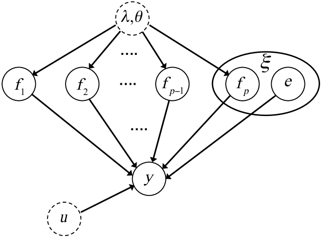
Figure 1: Bayesian network describing the stochastic model for linear system identification with (1) as measurements model. Solid and dotted nodes are, respectively, random and deterministic variables, with arrows to denote stochastic relationships. The nodes $f_{\ell}$ are the system impulse responses, given by zero-mean Gaussian processes with covariances given by $\lambda K_{\ell}$, where $K_{\ell}$ is the stable spline kernel possibly enriched with a small parametric part, while $\lambda$ is a scale factor. The vector $\theta$ contains the kernel parameters entering $K_{\ell}$. The nodes $y$, $u$ and $e$ indicate, respectively, the system output, the observable inputs and the innovation sequence of unit variance. Finally, the super node $\xi$ is the convolution between $e$ and $f_{p}$. It is defined by (12) and results in a stationary stochastic process with covariance given by the new class of RBF kernels defined in (13) in continuous-time, and in (17) in discrete-time.

4 Kernels for linear system identification

4.1 Stable spline kernels

In the literature on Gaussian regression, the adopted priors usually reflect only knowledge on the smoothness of the unknown function. One popular approach is to model it as the $q$-fold integral of white Gaussian noise. The resulting covariance becomes proportional to

$$W_{q}(s,t)=\int_{0}^{1}G_{q}(s,u)G_{q}(t,u)du$$ (9)

where

$$\\ G_{q}(r,u)=\frac{(r-u)_{+}^{m-1}}{(m-1)!},\qquad(u)_{+}=\left\{\begin{array}[]{cl}u&\mbox{if}~{}u\geq 0\\ 0&\mbox{otherwise}\end{array}\right.$$

This class contains the so-called spline kernels and underlies the Bayesian interpretation of $q$-th order smoothing splines, see [21] for details. One can see that the kernel $W$ does not account for impulse response stability: the variance of $f$ increases as time progresses.
In [3, 6] new kernels for linear system identification have been introduced to include the knowledge on smoothness and exponential BIBO stability. This is obtained by an exponential time transformation regulated by the hyperparameter $\beta>0$ which establishes how fast the variance of $f$ goes to zero. This leads to the following class of kernels parametrized by $q$:

$$K(s,t):=W_{q}(e^{-\beta s},e^{-\beta t}),\qquad m=1,2,\ldots.$$ (10)

The choice $q=1$ leads to $K(s,t)=e^{-\beta\max{(s,t)}}$. When $q=2$ one instead obtains the stable spline kernel originally introduced in [3], i.e.

$$K(s,t)=\frac{e^{-\beta(s+t)}e^{-\beta\max(s,t)}}{2}-\frac{e^{-3\beta\max(s,t)}}{6}$$ (11)

4.2 RBF kernels for linear system identification

According to our Bayesian paradigm, the impulse responses $f_{\ell}$ are modeled as Gaussian processes with covariance proportional to the stable spline kernel (11). Now, let us focus on the last component of the model (1). It involves $f_{p}$ and the noise $e$, and is given by

$$\xi(t):=(e\otimes f_{p})(t)$$ (12)

It is easy to see that $\xi$ is a (non Gaussian) zero-mean stationary stochastic process. As already mentioned at the beginning of the previous section, our aim is to define linear minimum variance estimators of the missing data. Hence, now we just need the second-order statistics of $\xi$. They are derived in the following proposition whose proof is not reported since it relies upon simple computations.

Proposition 1.

Consider the Bayesian network in Fig. 1. Let $f_{p}$ be a continuous-time zero-mean Gaussian process on ${\mathbb{R}}^{+}$ with covariance $\lambda K$, where $K$ is the stable spline kernel (10). It comes that $\xi$ in (12) is a zero-mean stationary stochastic process on ${\mathbb{R}}$, with covariance $\lambda R$ where

$$R(s,t) =h(s-t),\quad(s,t)\in{\mathbb{R}}\times{\mathbb{R}}$$ (13)

$$h(x) =\int_{0}^{+\infty}K(y,y+|x|)dy,\quad x\in{\mathbb{R}}$$

In particular, for $q=1$ one has

$$h(x)=\frac{e^{-\beta|x|}}{\beta}$$ (14)

while $q=2$ leads to

$$h(x)=\frac{3e^{-2\beta|x|}-e^{-3\beta|x|}}{18\beta}$$ (15)

Eq. (13) thus provides a new class of RBF kernels for identification, useful to describe system components subject to disturbances. Remarkably, the simplest element, obtained with $q=1$ and reported in (14), corresponds to the familiar Laplace kernel.

4.3 Stable spline and RBF kernels in discrete-time

It is straightforward to extend the results obtained in the previous two subsections to the discrete-time context. For what concerns the stable spline kernels (10), one can just consider their sampled versions

$$K(s,t):=W_{q}(e^{-\beta s},e^{-\beta t}),\qquad(s,t)\in{\mathbb{N}}\times{\mathbb{N}}$$ (16)

Then, starting from (16), the discrete-time versions of the RBF kernels (13) become

$$R(s,t) =h(s-t),\quad(s,t)\in{\mathbb{Z}}\times{\mathbb{Z}}$$ (17)

$$h(x) =\sum_{j=1}^{+\infty}K(j,j+|x|),\quad x\in{\mathbb{Z}}$$

In particular, for $q=1$ one has

$$h(x)=\frac{e^{-\beta(|x|+1)}}{1-e^{-\beta}}$$ (18)

while $q=2$, that corresponds to using (11), leads to

$$h(x)=\frac{3e^{-2\beta|x|}-e^{-3\beta|x|}}{6}\frac{e^{-3\beta}}{1-e^{-3\beta}}$$ (19)

4.4 Enriching the kernels and the ARMAX case

In some circumstances, it can be useful to add to the stable spline kernels (10) and (16) some components able to capture dynamics which are hardly represented by smooth processes, e.g. high-frequency poles. As described in [4], this goal can be obtained modeling each $f_{\ell}$ as

$$f_{\ell}=g_{\ell}\otimes h_{\ell}$$

where $g_{\ell}$ is a zero-mean Gaussian process, with covariance proportional to the stable spline kernel, while $h_{\ell}$ is a low-order parametric impulse response. Notice also that the definition of the new RBF kernels remains the same, except that $K$ in (13) and (17) has to be replaced by the stable spline kernel enriched with the parametric component.
For discrete-time ARMAX models, it is useful to set $h=h_{1}=\ldots=h_{p}$. In what follows, the zeta transform of $h$ is then given by

$$H(z)=\frac{z^{2}}{z^{2}+\phi z+\varphi}.$$

The overall model so depends on four hyper-parameters: $\phi$ and $\varphi$ which carry the information on the poles common to the impulse responses, the variance decay rate $\beta$ and the scale factor $\lambda$.

5 Stable spline imputation

5.1 Notation

In order to introduce the new imputation procedure, first we need to set up some additional notation.
Given the RBF kernel $R$ and the sampling instants $\{t_{i}\}_{i=1}^{n}$, $\mathbf{R}\in\mathbb{R}^{n\times n}$ is a positive semidefinite matrix, already introduced in (6), that we call RBF kernel matrix, whose $(i,j)$ entry is

$$[\mathbf{R}]_{ij}=R(t_{i},t_{j})$$ (20)

Given $K$ and the observable system inputs, the output kernel $P:\mathcal{X}\times\mathcal{X}\rightarrow{\mathbb{R}}$ is defined, for every $x,y\in\mathcal{X}$, by

$$P(x,y)=\sum_{\ell=1}^{p-1}\left(u_{\ell}\otimes h_{x}\right)(y)$$ (21)

where $h_{x}(t)$ is a function, parametrized by $x$, defined $\forall t$ by

$$h_{x}(t)=(u_{\ell}(\cdot)\otimes K(t,\cdot))(x)$$

Notice that, when performing the outer convolution, $h_{x}$ is thought of as a function parametrized by $x$. Furthermore, $\mathbf{P}\in\mathbb{R}^{n\times n}$ denotes the output kernel matrix whose $(i,j)$ entry is

$$[\mathbf{P}]_{ij}=P(t_{i},t_{j})$$ (22)

Remark 2.

When working in discrete-time, i.e. $\mathcal{X}={\mathbb{N}}$, $P(i,j)$ admits a simple expression using a matrix vector notation. In fact, let $\mathbf{K}^{\infty}_{\ell}$ denote the infinite-dimensional kernel matrix whose $(i,j)$ entry is

$$[\mathbf{K}^{\infty}_{\ell}]_{ij}=K_{\ell}(i,j),\quad(i,j)\in{\mathbb{N}}\times{\mathbb{N}}$$

Then, one obtains

$$P(i,j)=\sum_{\ell=1}^{p-1}\mathbf{U}^{i}_{\ell}\mathbf{K}^{\infty}_{\ell}\left(\mathbf{U}_{\ell}^{j}\right)^{\top}$$ (23)

where

$$\mathbf{U}^{i}_{\ell}=\left[u_{\ell}(i)\quad u_{\ell}(i-1)\quad u_{\ell}(i-2)\ldots\right]$$

Above, as in Section 2.3, notation of ordinary algebra has been adopted to handle infinite-dimensional objects.

5.2 Minimum variance linear estimator of the missing data

The next proposition provides the minimum variance linear estimator and the posterior covariance of the system output for known $\theta$ (see Appendix for the proof).

Proposition 3.

Consider the Bayesian model displayed in Fig. 1, where each $f_{\ell}$ is a zero-mean stochastic process of covariance $\lambda K$, with $K$ the stable spline kernel (10). Then, for known $\theta$ and arbitrary time instant $t$, the minimum variance linear estimator of $y(t)$ is

$$\hat{y}(t):=\hat{\mathbb{E}}[y(t)|\mathbf{y}_{o}]=\sum_{i=1}^{n}\hat{c}_{i}\left(P(t,t_{i})+R(t,t_{i})\right)$$ (24)

where the $\hat{c}_{i}$ are the components of the vector $\hat{\mathbf{c}}=\left(\mathbf{P}+\mathbf{R}\right)^{-1}\mathbf{y}_{o}.$ Finally, the posterior covariance of $y(t)$ given $\mathbf{y}_{o}$ is

$${\mathbb{V}}[y(t)|\mathbf{y}_{o}]=\lambda\left(P(t,t)+R(t,t)-a_{t}\left(\mathbf{P}+\mathbf{R}\right)^{-1}a_{t}^{\top}\right)$$ (25)

where $a_{t}=\left[P(t,t_{1})+R(t,t_{1})\quad\ldots\quad P(t,t_{n})+R(t,t_{n})\right].$

Eq. (24) thus makes available all the estimate of the system output in closed form. One can also see that the system output estimator has the structure of a particular regularization network [22]. It is a sum of $n$ basis functions with expansions coefficients obtained by solving a linear system of equations. Each basis function is the sum of the output kernel section $P(\cdot,t_{i})$, coming from the stable spline kernels convoluted with the system inputs, and of the RBF kernel section $R(\cdot,t_{i})$. Notice also that the estimate does not depend on the scale factor $\lambda$.

5.3 Stable spline imputation

In real applications, the estimator (24) can not be directly applied since it depends on the unknown vector $\theta$ entering the kernels $P$ and $R$. This problem can be faced exploiting the Bayesian framework underlying the stable spline estimator. In particular, $\theta$ can be estimated by optimizing the marginal likelihood, i.e. the joint density of $\mathbf{y}_{o}$ and the impulse responses $f_{\ell}$, where the impulse responses are integrated out. Adopting a Gaussian approximation for the disturbance, then using the same arguments adopted in Appendix of [4], the estimate of $\theta$ becomes

$$\hat{\theta} =\arg\min_{\theta}J(\theta)$$ (26a)

$$J(\theta) =\mathbf{y}_{o}^{\top}(\lambda\mathbf{P}+\lambda\mathbf{R})^{-1}\mathbf{y}_{o}+\log\det(\lambda\mathbf{P}+\lambda\mathbf{R})$$ (26b)

Our numerical procedure, namely stable spline imputation, able to return any missing output sample is then given below.

Algorithm 4 (Stable Spline Imputation).

The input to this algorithm includes the system inputs $u_{\ell}$, the sampling instants $\{t_{i}\}_{i=1}^{n}$, and the measurement vector $\mathbf{y}_{o}$. The output of this algorithm is the estimate $\hat{y}(t)$, where $t$ denotes the time instant where the system output needs to be estimated. The steps are as follows:

• Compute the hyperparameter vector via marginal likelihood optimization as described in (26).

• Set the hyperparameter vector $\theta$ to $\hat{\theta}$ and return the following estimate of $y(t)$:

  $$\hat{y}(t)=\sum_{i=1}^{n}\hat{c}_{i}\left(P(t,t_{i})+R(t,t_{i})\right)$$

  where the $\hat{c}_{i}$ are the components of the vector

  $$\hat{\mathbf{c}}=\left(\mathbf{P}+\mathbf{R}\right)^{-1}\mathbf{y}_{o}$$

Usual parametric approaches to imputation must solve several non convex optimization problems, possibly in high-dimensional spaces. This e.g. happens adopting rational transfer functions of unknown order so that it is necessary consider various model parameterizations, possibly involving vectors with tens/hundreds of components. In the stable spline imputation procedure, model order is instead encoded in the hyperparameter vector $\theta$. Hence, only $J$ must be optimized. Any evaluation of such objective requires $O(nq^{2})$ operations using $q$ to denote the number of estimated coefficients of the one-step ahead predictor, e.g. see [8] for details on marginal likelihood computation. Once $\theta$ is known, the solution is then available in closed form. When ARMAX models are e.g. considered, $\theta$ contains only $(\beta,\lambda)$ or, at the most, also the other two parameters $(\phi,\varphi)$ describing two poles. Thus, a two or a four-dimensional space needs to be explored so that, even if the objective is non-convex, grid methods could be also adopted to mitigate the risk of local minima.

6 Numerical experiments

6.1 Identification of discrete-time ARMAX models

Let us now consider a Monte Carlo study of 500 runs. During each run a discrete-time ARMAX linear system with $3$ observable inputs is randomly generated as follows:

• each rational transfer function is given the same order, randomly chosen in $\{1,2,...,30\}$;

• the polynomials defining the model are generated using the MATLAB function drmodel.m. The system and the predictor poles are restricted to have modulus less than 0.95 with the ratio between the sum of the $\ell_{2}$ norms of $f_{\ell}$, $\ell=1,2,3$, and of $f_{4}$ falling in $[1,5]$ (drmodel.m is repeatedly called at any run until such requirements are fulfilled). The delay between all the inputs and the output is always equal to 1.

Independent realizations of unit variance white noises are used as inputs. Output data are collected after getting rid of initial conditions to define a training set of 300 input-output pairs and a test set of size 1000. To simulate a missing data problem, at every run the training set is reduced by randomly discarding an output value with probability 0.25.

6.2 Performance measures

Two performance measures will be used to compare the performance of different estimators. The first index is the quality in the reconstruction of the missing data contained in the vector ${\bf y}_{m}$. It is given by the Coefficient of Determination $COD_{miss}$, computed at any run as

$$COD_{miss}=1-\frac{\|{\bf y}_{m}-\hat{\bf y}_{m}\|^{2}}{\|{\bf y}_{m}-\bar{{\bf y}}_{m}\|^{2}}$$ (27)

where $\|\cdot\|$ is the Euclidean norm and $\bar{{\bf y}}_{m}$ indicates the average value of the components of ${\bf y}_{m}$.
The second index measures the ability of the estimated model in predicting the test set, as a function of the prediction horizon $k$. In particular, we use the $k$-step ahead Coefficient of Determination, denoted by $COD_{k}$ for $k=1,2,\ldots,20$, and computed at any run as follows:

$$COD_{k}=1-\frac{\|{\bf y}_{test}-\hat{\bf y}_{test}^{k}\|^{2}}{\|{\bf y}_{test}-\bar{{\bf y}}_{test}\|^{2}},\quad k=1,2,\ldots,20$$ (28)

where ${\bf y}_{test}$ is the vector containing the outputs in the test set, whose sample mean is denoted by $\bar{{\bf y}}_{test}$, while the components of the vector $\hat{\bf y}_{test}^{k}$ are the $k$-step ahead predictions computed using the estimated model. The average of the values of $COD_{k}$ obtained after the 500 Monte Carlo runs is then denoted by $\overline{COD}_{k}$.

6.3 The adopted estimators

The following 6 estimators are used:

• PEM+Oracle (missing): This algorithm computes the PEM (ML in the Gaussian case) estimator of the system parameters; the Prediction Error cost is computed using the Kalman filter (see, e.g. [9]). Note that, alternatively, the same result would have been obtained formulating it as a missing data problem by adding the missing observations as unknowns and then using the EM algorithm, which iterates between computing conditional expectation of the conditional log likelihood over the missing data for fixed model parameters and maximizing of the expected log likelihood [16, 17]. The procedure is repeated for all ARMAX models with the three polynomials with the same degree ranging from 1 to 20 (increasing this number does not improve the results); the model order selection is then performed by an oracle which, at each run, maximizes $COD_{k}$ and $COD_{miss}$. Notice that the chosen orders depend on the target, i.e. prediction quality on a certain horizon $k$ or quality in the reconstruction of the missing data. The same order selection procedure is used also when the other PEM-based approaches described below are used. The missing data are then estimated using a Rauch-Tung-Striebel smoother based on the estimated model parameters, which are the maximum a posteriori estimates of the missing observations conditionally on the estimated model and the observed data.

• PEM+Oracle (full): the same as above, except that the estimator uses all the 300 identification data and the pem.m function of the MATLAB System Identification Toolbox is used to estimate the model.

• PEM+BIC (full): the same as above, except that BIC is used for model order selection.

• PEM+AICC (full): the same as above except that the corrected version of Akaike criterion (AICC) [23] is used for model order selection.

• SS (full): this is the Stable Spline estimator described in [4] to which the reader is referred for all the details. Here, we just recall that the stable spline kernel of order $q=2$ enriched with a parametric part describing two poles is used. Hence, the dimension of the hyperparameter vector is 4 and its components are estimated via marginal likelihood optimization. For computational reasons, the number of estimated coefficients of the one-step predictor impulse responses is set to 100. To form the regression matrices, entries depending on samples values at time instants $t<t_{1}$ are set to zero, even if data are not generated starting from null initial conditions.

• SS imputation+SS: this estimator has to identify the system using the reduced training set. First, the stable spline imputation procedure defined by Algorithm 4 is used to recover the missing output values. Then, the ARMAX model is estimated using the Stable Spline estimator fed with the union of the available measurements and the estimated outputs as returned by Algorithm 4. Also in this case, regression matrices’ entries depending on samples values at time instants $t<t_{1}$ are set to zero.

The information that the delay between all the inputs and the output is equal to 1 is provided to all the system identification algorithms listed above. Notice that all the estimators exploit the full data set of 300 samples, except PEM+Oracle (missing), and SS imputation+SS which, on average, use only 225 output measurements.

6.4 SS imputation+SS vs PEM+Oracle (missing)

We start comparing the performance of PEM+Oracle (missing), and SS imputation+SS which are the two estimators which have to handle missing data situations.
The top panel of Fig. 2 displays results regarding the prediction capability of the estimated models. In particular, the abscissae and the ordinates of the 2000 points contained in the figure correspond to the values of $\{COD_{k}\}_{k=1}^{20}$ returned, respectively, by PEM+Oracle (missing) and SS imputation+SS after the first 100 runs. It turns out the the predictive performance of SS imputation+SS is superior to that of the oracle-based procedure in almost $87\%$ of the cases. This result is remarkable since the oracle uses additional information not available to SS imputation+SS to select that model order (function of $k$) which maximizes $COD_{k}$ or $COD_{miss}$.
The bottom panel of Fig. 2 compares the quality in the reconstruction of ${\bf{y}}_{m}$ by reporting the MATLAB boxplots of the values of $COD_{miss}$ returned by the two estimators after the 500 runs. One can see that the performance of the stable spline imputation (which is implementable in real applications) is very similar to that of PEM+Oracle (missing) (which is not implementable in practice).

6.5 SS imputation+SS vs estimators using the full data set

We now compare the performance of SS imputation+SS with that of all the other estimators exploiting the full data set. The top panel of Fig. 3 displays $\overline{COD}_{k}$ achieved by the 5 estimators after the 500 runs, as a function of the prediction horizon. The bottom panel display the boxplots of the 500 values of $COD_{5}$. The mean performance of the new estimator SS imputation+SS, is comparable to that of SS (full) which provides result similar of those of PEM+Oracle (full).

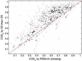
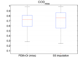
Figure 2: ARMAX identification (subsection 6.4). Top: assessment of models prediction capability. Values of $\{COD_{k}\}_{k=1}^{20}$ returned by PEM+Oracle (missing) ($x$-axis) vs those returned by SS imputation+SS ($y$-axis) after the first 100 runs. Bottom: assessment of quality in missing data reconstruction. MATLAB boxplots of the values of $COD_{miss}$ obtained after the 500 Monte Carlo runs.

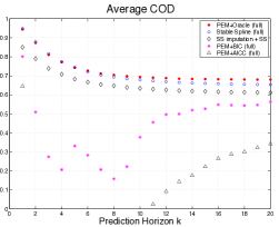
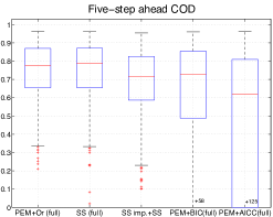
Figure 3: ARMAX identification (subsection 6.5). Top: $\overline{COD}_{k}$, i.e. average coefficient of determination relative to $k$-step ahead prediction, using PEM+Oracle (full) ($\bullet$), Stable Spline (full) ($\circ$), SS imputation+SS ($\Diamond$), PEM+BIC (full) ($\ast$) and PEM+AICC (full) ($\triangle$). Bottom: boxplots of the 1000 values of $COD_{5}$. Recall that all the estimators, except SS imputation+SS, exploit all the identification data.

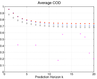
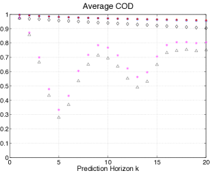
Figure 4: Variants of the ARMAX identification experiment using either a lowpass input in place of white noise (left) or inserting a couple of lowly damped poles in the system impulse responses (subsection 6.6). The figures shows $\overline{COD}_{k}$, i.e. average coefficient of determination relative to $k$-step ahead prediction, using PEM+Oracle (full) ($\bullet$), Stable Spline (full) ($\circ$), SS imputation+SS ($\Diamond$), PEM+BIC (full) ($\ast$) and PEM+AICC (full) ($\triangle$). Recall that all the estimators, except SS imputation+SS, exploit all the identification data.

6.6 Variants of the experiment

We have also considered two variants of the experiment. In the first one, in place of white noises, the observable system inputs are given by low pass signals. In particular, the inputs are independent realizations of white noises filtered by a strictly proper second-order rational transfer function randomly generated at every run (the same mechanism used to generate the system impulse responses is used). In the second one, the system and the predictor poles are restricted to have modulus less than 0.999 (in place of 0.95) and, in addition, the unknown system impulse responses have been enriched by adding to them a couple of lowly damped poles. In particular, each transfer function is that obtained by the MATLAB generator multiplied by

$$\frac{z^{2}}{z^{2}+2abz+b^{2}}$$

where $b=0.999$ while $a$ is, at every run, a different realization from a uniform distribution on $[-1,1]$. The left and right panels of Fig. 4 displays $\overline{COD}_{k}$ following the same rationale adopted in Fig. 2. As a matter of fact, in both the variants, the stable spline estimators still outperform the classical system identification approaches also when the latter exploit the full data set.

7 Conclusions

In this paper we have shown that stable spline kernels can be used also to derive a new class of RBF covariances useful to model that part of the system output due to disturbances. The stable spline and the new RBF kernels lead to a new solution of the missing data problem based on a new imputation procedure, namely stable spline imputation. It returns all the missing output samples just solving one low-dimensional optimization problem.
The new technique has been used to identify discrete-time ARMAX models under missing data. In many cases of interest the new stable spline imputation followed by the stable spline estimator developed in [4] may return models more predictive than those obtained by standard parametric PEM, also when the latter have access to the full data set.

Appendix: Proof of Proposition 3

The proof relies upon well known results regarding the estimation of stochastic processes, e.g. see [20]. The minimum variance linear estimator of $y(t)$ given $\mathbf{y}_{o}$ is

$$\hat{y}(t)={\mathbb{V}}(y(t),\mathbf{y}_{o})\left({\mathbb{V}}(\mathbf{y}_{o})\right)^{-1}\mathbf{y}_{o}$$

Now, recall that the innovation $e$ and the $\{f_{\ell}\}_{\ell=1}^{p}$ are all assumed mutually independent. This implies also the independence of $\xi$ and $\{f_{\ell}\}_{\ell=1}^{p-1}$. Thus, we obtain ${\mathbb{V}}(\mathbf{y}_{o})=\lambda\left(\mathbf{P}+\mathbf{R}\right)$ and one also has

$${\mathbb{V}}(y(t),\mathbf{y}_{o})=\lambda\left(P(t,t_{1})+R(t,t_{1}),\ldots,P(t,t_{n})+R(t,t_{n})\right)$$

so that (24) is obtained. Similar arguments lead to (25) and this completes the proof.
of Proposition 3.

References

- [1] L. Ljung, System Identification - Theory For the User. Prentice Hall, 1999.
- [2] H. Akaike, “A new look at the statistical model identification,” IEEE Transactions on Automatic Control, vol. 19, pp. 716–723, 1974.
- [3] G. Pillonetto and G. De Nicolao, “A new kernel-based approach for linear system identification,” Automatica, vol. 46, pp. 81–93, 2010.
- [4] G. Pillonetto, A. Chiuso, and G. De Nicolao, “Prediction error identification of linear systems: A nonparametric Gaussian regression approach,” Automatica, vol. 47, pp. 291–305, 2011.
- [5] C. Rasmussen and C. Williams, Gaussian Processes for Machine Learning. The MIT Press, 2006.
- [6] G. Pillonetto, A. Chiuso, and G. De Nicolao, “Regularized estimation of sums of exponentials in spaces generated by stable spline kernels,” in Proceedings of the 2010 American Control Conference, Baltimora, 2010.
- [7] T. Chen, H. Ohlsson, and L. Ljung, “On the estimation of transfer functions, regularizations and Gaussian processes - revisited,” Automatica, vol. 48, no. 8, pp. 1525–1535, 2012.
- [8] G. Pillonetto, F. Dinuzzo, T. Chen, G. D. Nicolao, and L. Ljung, “Kernel methods in system identification, machine learning and function estimation: a survey,” Automatica, vol. 50, no. 3, pp. 657–682, 2014.
- [9] R. Jones, “Maximum likelihood fitting of arma models to time series with observations,” Technometrics, vol. 22, pp. 389–395, 1980.
- [10] C. F. Ansley and R. Kohn, “Exact likelihood of vector autoregressive-moving average process with missing or aggregated data,” Biometrika, vol. 70, no. 1, pp. 275–278, 1983.
- [11] J. Penzer and B. Shea, “The exact likelihood of an autoregressive-moving average model with incomplete data,” Biometrika, vol. 84, no. 4, pp. 919–928.
- [12] P. Broersen, S. de Waele, and R. Bos, “Autoregressive spectral analysis when observations are missing,” Automatica, vol. 40, pp. 1495–1504, 2004.
- [13] W. Gilks, S. Richardson, and D. Spiegelhalter, Markov chain Monte Carlo in Practice. London: Chapman and Hall, 1996.
- [14] W. Dunsmuir and P. Robinson, “Estimation of time series models in the presence of missing data,” Journal of the American Statistical Association, vol. 76, pp. 560–568, 1981.
- [15] R. Pintelon and J. Schoukens, “Frequency domain system identification with missing data,” IEEE Transactions on Automatic Control, vol. 45, pp. 364–369, 2000.
- [16] A. P. Dempster, N. M. Laird, and D. B. Rubin, “Maximum likelihood from incomplete data via the em algorithm,” Journal of the Royal Statistical Society. Series B (Methodological), vol. 39, no. 1, pp. 1–38, 1977. [Online].
- [17] A. Isaksson, “Identification of ARX models subject to missing data,” IEEE Transactions on Automatic Control, vol. 38, pp. 813–819, 1993.
- [18] T. Soderstrom and P. Stoica, System Identification. Prentice Hall, 1989.
- [19] G. Pillonetto and A. Chiuso, “A Bayesian learning approach to linear system identification with missing data,” in Proceedings of the 48th IEEE International Conference on Decision and Control, S. Mendelson and A. J. Smola, Eds., Shangai, China, 2009.
- [20] B. D. O. Anderson and J. B. Moore, Optimal Filtering. Englewood Cliffs, N.J., USA: Prentice-Hall, 1979.
- [21] G. Wahba, Spline models for observational data. SIAM, Philadelphia, 1990.
- [22] T. Poggio and F. Girosi, “Networks for approximation and learning,” in Proceedings of the IEEE, vol. 78, 1990, pp. 1481–1497.
- [23] C. Hurvich and C. Tsai, “Regression and time series model selection in small samples,” Biometrika, vol. 76, pp. 297–307, 1989.
- [24] M. Bisiacco and G. Pillonetto. On the Mathematical foundations of stable RKHSs. Automatica, 2020.
- [25] M. Bisiacco and G. Pillonetto. Kernel absolute summability is sufficient but not necessary for RKHS stability. SIAM Journal on Control and Optimization, 2020.
- [26] G. Bottegal, A.Y. Aravkin, H. Hjalmarsson, and G. Pillonetto. Robust EM kernel-based methods for linear system identification. Automatica, 67:114 – 126, 2016.
- [27] T. Chen. On kernel design for regularized lti system identification. Automatica, 90:109 – 122, 2018.
- [28] T. Chen, M. S. Andersen, L. Ljung, A. Chiuso, and G. Pillonetto. System identification via sparse multiple kernel-based regularization using sequential convex optimization techniques. IEEE Transactons on Automatic Control, provisionally accepted, 2013.
- [29] T. Chen, L. Ljung, M. Andersen, A. Chiuso, F.P. Carli, and G. Pillonetto. Sparse multiple kernels for impulse response estimation with majorization minimization algorithms. In IEEE Conference on Decision and Control, pages 1500–1505, Hawaii, Dec 2012.
- [30] T. Chen and G. Pillonetto. On the stability of reproducing kernel Hilbert spaces of discrete-time impulse responses. Automatica, 95:529 – 533, 2018.
- [31] A. Chiuso, T. Chen, L. Ljung, and G. Pillonetto. Regularization strategies for nonparametric system identification. In Proceedings of the 52nd Annual Conference on Decision and Control (CDC), 2013.
- [32] M.A.H. Darwish, G. Pillonetto, and R. Toth. The quest for the right kernel in Bayesian impulse response identification: The use of obfs. Automatica, 87:318 – 329, 2018.
- [33] F. Dinuzzo. Kernels for linear time invariant system identification. SIAM Journal on Control and Optimization, 53(5):3299–3317, 2015.
- [34] L. Ljung, T. Chen, and B. Mu. A shift in paradigm for system identification. International Journal of Control, pages 1–8, 2019.
- [35] G. Pillonetto. Consistent identification of Wiener systems: A machine learning viewpoint. Automatica, 49(9):2704–2712, September 2013.
- [36] G. Pillonetto. A new kernel-based approach to hybrid system identification. Automatica, 70:21 – 31, 2016.
- [37] G. Pillonetto. System identification using kernel-based regularization: New insights on stability and consistency issues. Automatica, 93:321–332, 2018.
- [38] G. Pillonetto, T. Chen, A. Chiuso, G. De Nicolao, and L. Ljung. Regularized linear system identification using atomic, nuclear and kernel-based norms: The role of the stability constraint. Automatica, 69:137 – 149, 2016.
- [39] G. Pillonetto and A. Chiuso. Tuning complexity in regularized kernel-based regression and linear system identification: The robustness of the marginal likelihood estimator. Automatica, 58:106 – 117, 2015.