Limit cycles in periodically driven open quantum systems

Abstract

We investigate the long-time behavior of quantum $N$-level systems that are coupled to a Markovian environment and subject to periodic driving. As our main result, we obtain a general algebraic condition ensuring that all solutions of a periodic quantum master equation with Lindblad form approach a unique limit cycle. Quite intuitively, this criterion requires that the dissipative terms of the master equation connect all subspaces of the system Hilbert space during an arbitrarily small fraction of the cycle time. Our results provide a natural extension of Spohn’s algebraic condition for the approach to equilibrium to systems with external driving.

1 Introduction and Main Result

The theory of open quantum systems provides us with powerful tools to describe the dynamics of quantum-mechanical objects that interact with a macroscopic environment [1]. A cornerstone of this framework is the Gorini–Kossakowski–Sudarshan–Lindblad (GKSL) equation,

$$\partial_{t}\rho_{t}=\hat{L}_{t}\rho_{t}\equiv\frac{1}{\rmi\hbar}[H_{t},\rho_{t}]+\sum_{\mu=1}^{M_{t}}\gamma^{\mu}_{t}\Big{(}A^{\mu}_{t}\rho_{t}A^{\mu\dagger}_{t}-\frac{1}{2}A^{\mu\dagger}_{t}A^{\mu}_{t}\rho_{t}-\frac{1}{2}\rho_{t}A^{\mu\dagger}_{t}A^{\mu}_{t}\Big{)}.$$ (1)

Under certain technical conditions, this equation of motion defines the most general Markovian, i.e., memoryless, time evolution of a physical state $\rho_{t}$ [2, 3, 4, 5]. The self-adjoint operator $H_{t}$ is thereby usually identified with the effective Hamiltonian of the system, while the influence of the environment is encoded in the Lindblad operators $A^{\mu}_{t}$ with corresponding coupling rates $\gamma^{\mu}_{t}>0$; $\hbar$ denotes Planck’s constant. Notably, all components of the Lindblad generator $\hat{L}_{t}$, including the number of dissipation channels $M_{t}$, can be time-dependent if the system is externally driven.

Owing to its high degree of generality, the GKSL equation has found application in nearly all areas of modern quantum physics ranging from quantum optics [6] and quantum information theory [7, 8] over quantum thermodynamics [9, 10, 11] to quantum device engineering [12]. The general mathematical properties of this equation, which have been extensively studied over the last decades [13, 14, 15, 16, 17, 18, 19], have thus become a source of valuable physical insight. A particularly important problem in this context is to characterize the long-time behavior of its solutions. For systems without external driving, which are described by a time-independent Lindblad generator, the conditions that lead to a unique stationary limiting state $\rho^{\mathrm{ss}}$ are well understood [5]. In particular, Spohn proved a general criterion that, quite intuitively, requires the dissipative terms of the Lindblad generator to connect all subspaces of the system Hilbert space [20]. This result can be formulated as follows:

Theorem 1 (Spohn).

For a system obeying the GKSL equation (1) with time-independent Lindblad generator $\hat{L}$, let $\mathcal{A}\equiv\operatorname{span}\{A^{1}\dots A^{M}\}$ be the linear span of all Lindblad operators. If $\mathcal{A}$ is self-adjoint and irreducible, then there exists a unique state $\rho^{\mathrm{ss}}$ so that

$$\lim_{t\to\infty}\left(\rho_{t}-\rho^{\mathrm{ss}}\right)=0$$ (2)

for arbitrary initial conditions $\rho_{0}$. Here, $\mathcal{A}$ is self-adjoint if $X^{\dagger}\in\mathcal{A}$ for all $X\in\mathcal{A}$ and irreducible if $[X,Y]=0$ for all $X\in\mathcal{A}$ implies that $Y$ is a multiple of the identity.

The central aim of this letter is to extend this theorem to periodically driven systems, whose Lindblad generator is explicitly time-dependent and obeys the condition $\hat{L}_{t+T}=\hat{L}_{t}$ for some cycle time $T$. Such systems are commonly studied in quantum thermodynamics, for example as models of cyclic thermal machines [9, 21, 10].

When a periodic driving protocol is constantly applied to a dissipative system, we intuitively expect its state $\rho_{t}$ to approach a periodic limit cycle satisfying $\rho^{\mathrm{cy}}_{t+T}=\rho^{\mathrm{cy}}_{t}$. This expectation can be motivated using the following argument given in [9]. The relative entropy between two states $\rho_{t}$ and $\sigma_{t}$ is defined as

$$S(\rho_{t}\|\sigma_{t})=-\tr[\rho_{t}\,(\log\rho_{t}-\log\sigma_{t})].$$ (3)

Being non-negative and zero only if $\rho_{t}=\sigma_{t}$, this quantity can be understood as a distance measure on the state space of a given system. The dynamics induced by the GKSL equation can only decrease the relative entropy between two states, i.e., $S(\rho_{\tau}\|\sigma_{\tau})\leq S(\rho_{t}\|\sigma_{t})$ for any time $\tau>t$ [1]. Using this result with $\sigma_{t}=\rho_{t+T}$ and $\tau=t+T$ yields $S(\rho_{t+T}\|\rho_{t+2T})\leq S(\rho_{t}\|\rho_{t+T})$. Hence, the relative entropy between $\rho_{t}$ and $\rho_{t+T}$ decreases with every period.

This argument implies that the relative entropy between $\rho_{t}$ and $\rho_{t+T}$ converges to a limit value at long times. We can, however, not conclude that this value is zero, i.e., that $\rho_{t}=\rho_{t+T}$. In fact, there are periodically driven open quantum systems described by GKSL equations, for which the period length of the system response at long times is an integer multiple of the applied cycle time $T$, see for example [22]. Furthermore, the argument given above cannot be used to address the uniqueness of the limit cycle. It thus remains unclear which conditions must be met for the long-time solution of (1) to be a unique limit cycle satisfying $\rho^{\mathrm{cy}}_{t+T}=\rho^{\mathrm{cy}}_{t}$. Here, we show that, to this end, it suffices that the periodic Lindblad generator $\hat{L}_{t}$ satisfies the requirements of Theorem 1 for an arbitrarily small fraction of the period $T$. As our main result, we obtain the following theorem:

Theorem 2.

Consider a system obeying the GKSL equation (1) with periodic Lindblad generator, $\hat{L}_{t+T}=\hat{L}_{t}$. Assume there is a $\tau\in(0,T]$ so that $\hat{L}_{t}$ is continuous on $[0,\tau]$, and $\mathcal{A}_{t}\equiv\operatorname{span}\{A^{1}_{t}\dots A^{M_{t}}_{t}\}$ is self-adjoint and irreducible for all $t\in[0,\tau]$. Then there exists a unique limit cycle $\rho^{\mathrm{cy}}_{t}=\rho^{\mathrm{cy}}_{t+T}$ so that

$$\lim_{t\to\infty}\left(\rho_{t}-\rho^{\mathrm{cy}}_{t}\right)=0$$ (4)

for arbitrary initial conditions $\rho_{0}$.

We proceed as follows. After fixing the notation in Section 2, we briefly review the proof of Theorem 1 in Section 3. In Section 4, we derive our main result. Further aspects are considered in our concluding Section 5.

2 Setup and Notation

We consider an open quantum system with finite-dimensional Hilbert space $\mathcal{H}$. The space of linear, self-adjoint operators $X:\mathcal{H}\to\mathcal{H}$ is denoted by $\mathcal{S}$ and equipped with the trace-norm

$$\|X\|_{1}\equiv\sum_{\lambda\in\sigma(X)}|\lambda|,$$ (5)

where $\sigma(X)$ is the set of eigenvalues of $X$. Upon introducing the Hilbert-Schmidt inner product,

$$\langle X,Y\rangle\equiv\tr[XY],$$ (6)

$\mathcal{S}$ becomes a Hilbert space [23]. Linear operators $\hat{V}:\mathcal{S}\to\mathcal{S}$ are called superoperators and indicated by hats; $\hat{V}^{\dagger}$ denotes the Hermitian adjoint of $\hat{V}$ with respect to the scalar product (6). The operator norm of a superoperator with respect to the trace-norm is defined as

$$\|\hat{V}\|_{1}\equiv\max_{X\in\mathcal{S},\,X\neq 0}\frac{\|\hat{V}X\|_{1}}{\|X\|_{1}}.$$ (7)

Throughout this letter, we use the symbol $\rho$ to denote the state of the system, i.e., a positive operator in $\mathcal{S}$ satisfying $\tr\rho=1$.

3 Time-Independent Lindblad Generators

In this section, we sketch Spohn’s proof of Theorem 1 [20]. We consider an open quantum system obeying the GKSL equation (1) with constant generator $\hat{L}_{t}=\hat{L}$. The formal solution of this differential equation is given by $\rho_{t}=\hat{V}_{t}\,\rho_{0}$, where the set of propagators $\hat{V}_{t}\equiv\rme^{\hat{L}t}$ forms a quantum dynamical semigroup. To prove Theorem 1, we will show that $\hat{L}$ has exactly one zero eigenvalue and that all other eigenvalues of $\hat{L}$ have negative real parts.

Recall that $\mathcal{A}\equiv\operatorname{span}\{A^{1}\dots A^{M}\}$ denotes the linear span of the Lindblad operators. Since $\mathcal{A}$ is self-adjoint by assumption, there is an orthonormal set of Hermitian operators $\{F^{1}\dots F^{m}\}\subset\mathcal{S}$ with $m\leq M$ that spans $\mathcal{A}$, i.e., we have $A^{\mu}\equiv\sum_{\alpha=1}^{m}c_{\mu\alpha}F^{\alpha}$ for some complex coefficients $c_{\mu\alpha}$. Upon inserting this expansion into (1), the Lindblad generator takes the form

$$\hat{L}\rho=\frac{1}{\rmi\hbar}[H,\rho]+\sum_{\alpha,\beta=1}^{m}B_{\alpha\beta}\,\Big{(}F^{\alpha}\rho F^{\beta}-\frac{1}{2}F^{\beta}F^{\alpha}\rho-\frac{1}{2}\rho F^{\beta}F^{\alpha}\Big{)},$$ (8)

where $B_{\alpha\beta}\equiv\sum_{\mu=1}^{M}\gamma^{\mu}c_{\mu\alpha}c_{\mu\beta}^{\ast}$. By construction, the coefficient matrix $B_{\alpha\beta}$ is positive definite. Hence, its smallest eigenvalue $b$ is strictly positive. We now separate the diagonal contribution

$$\hat{L}_{\mathrm{d}}\,\rho\equiv\frac{b}{2}\,\sum_{\alpha=1}^{m}\Big{(}F^{\alpha}\rho F^{\alpha}-\frac{1}{2}F^{\alpha}F^{\alpha}\rho-\frac{1}{2}\rho F^{\alpha}F^{\alpha}\Big{)}$$ (9)

from the generator (8), such that $\hat{L}\equiv\hat{L}_{\mathrm{d}}+\hat{L}_{\mathrm{r}}$.

Using the irreducibility of $\mathcal{A}$, it is straightforward to show that the superoperator $\hat{L}_{\mathrm{d}}$ has exactly one zero eigenvalue corresponding to the eigenvector $\mathbbm{1}$, and that its remaining eigenvalues are negative [20]. We now denote by $-\lambda$ the maximum non-vanishing eigenvalue of $\hat{L}_{\mathrm{d}}$ and by $\hat{L}^{\prime}$, $\hat{L}_{\mathrm{d}}^{\prime}$ and $\hat{L}_{\mathrm{r}}^{\prime}$ the restrictions of $\hat{L}$, $\hat{L}_{\mathrm{d}}$ and $\hat{L}_{\mathrm{r}}$ to $\mathbbm{1}^{\perp}$, the orthogonal complement of $\mathbbm{1}$ in $\mathcal{S}$, i.e., the subspace of traceless operators. Since $\hat{L}_{\mathrm{d}}$ is self-adjoint, we can conclude that

$$\|\exp[\hat{L}_{\mathrm{d}}^{\prime}t]\,\|_{1}^{\prime}\leq\rme^{-\lambda t}.$$ (10)

Here, $\|\bullet\|_{1}^{\prime}$ is the operator norm with respect to the trace-norm on $\mathbbm{1}^{\perp}$.

Next, we consider the remaining generator $\hat{L}_{\mathrm{r}}$. By construction, this superoperator is still the generator of a quantum dynamical semigroup. Hence, the corresponding propagator $\exp[\hat{L}_{\mathrm{r}}t]$ is completely positive and trace preserving and therefore contractive, i.e., $\|\exp[\hat{L}_{\mathrm{r}}t]\,\|_{1}=1$ [5]. Since the image of $\hat{L}_{\mathrm{r}}$ is contained in $\mathbbm{1}^{\perp}$, we find that

$$\|\exp[\hat{L}_{\mathrm{r}}^{\prime}t]\,\|_{1}^{\prime}\leq\|\exp[\hat{L}_{\mathrm{r}}t]\,\|_{1}=1.$$ (11)

Combining this bound with (10) by means of the Lie product formula [23], we obtain

$$\|\exp[\hat{L}^{\prime}t]\,\|_{1}^{\prime}\leq\lim_{N\to\infty}\Big{(}\left\|\,\exp[\hat{L}_{\mathrm{s}}^{\prime}\,t/N]\,\exp[\hat{L}_{\mathrm{a}}^{\prime}\,t/N]\,\right\|_{1}^{\prime}\Big{)}^{N}\leq\rme^{-\lambda t}.$$ (12)

Thus, all eigenvalues of $\hat{L}^{\prime}$ have negative real parts.

Finally, we choose an orthonormal basis of $\mathcal{S}$ with $(\dim\mathcal{H})^{-1/2}\,\mathbbm{1}$ being the first basis element. The matrix representation of $\hat{L}$ in such a basis has the form

$$\hat{L}=\Bigg{[}\!\begin{array}[]{cc}0&0\cdots 0\\ \ast&(\hat{L}^{\prime})\end{array}\!\Bigg{]},$$ (13)

where $\ast$ denotes unknown entries. Examining the characteristic polynomial of this matrix proves first that $\hat{L}$ has a single zero eigenvalue and second that the remaining eigenvalues are identical to the eigenvalues of $\hat{L}^{\prime}$, which have negative real parts. The proof of Theorem 1 is thus complete.

4 Periodic Lindblad Generators

We now move on to driven systems with a time-periodic Lindblad generator $\hat{L}_{t+T}=\hat{L}_{t}$. The propagator $\hat{V}_{t,t_{0}}$, which maps the initial state $\rho_{t_{0}}$ to the later state $\rho_{t}$, here depends on both the initial and the final time. Our goal is to show that $\rho_{t}$ approaches a limit cycle $\rho^{\mathrm{cy}}_{t+T}=\rho^{\mathrm{cy}}_{t}$ at long times. A direct approach to this problem is, however, complicated by the fact that the limit cycle can generally not be explicitly determined.

To circumvent this difficulty, we work in the Heisenberg picture, where the state $\rho_{0}$ is constant and the observables $X\in\mathcal{S}$ carry the time dependence $X_{t}=V_{t,0}^{\dagger}X_{0}$. Note that the time evolution of $X_{t}$ does generally not follow from a time-local differential equation [1]. In order to prove Theorem 2, it suffices to show that any observable $X_{t}$ becomes a multiple of the identity at long times, $X_{t}=x_{t}\mathbbm{1}$ for some scalar $x_{t}=x_{t+T}$; the expectation value $\langle X_{t}\rangle\equiv\tr[X_{t}\,\rho_{0}]$ then becomes periodic and independent of the initial state.

The eigenvalues of $\hat{L}_{t}^{\dagger}$ are the complex conjugates of the eigenvalues of $\hat{L}_{t}$. Therefore, they all have a negative real part, except for a single zero eigenvalue with constant eigenvector $\mathbbm{1}$. This fact is, however, not sufficient to conclude that $X_{t}$ becomes a multiple of the identity at long times, since the adjoint generators $\hat{L}_{t_{1}}^{\dagger}$ and $\hat{L}_{t_{2}}^{\dagger}$ at different times $t_{1}$ and $t_{2}$ do not commute with each other in general. Instead, the strategy of our proof is to introduce a norm for $X_{t}^{\prime}$, the orthogonal projection of $X_{t}$ on $\mathbbm{1}^{\perp}$, which strictly decreases whenever $\hat{L}_{t}$ satisfies the conditions of Theorem 1.

To this end, we first consider a general subspace $\mathcal{S}^{\prime}$ of $\mathcal{S}$, and define

$$\|X\|_{\infty}\equiv\max\left\{|\langle Y,X\rangle|:\|Y\|_{1}=1,Y\in\mathcal{S}^{\prime}\right\}$$ (14)

for $X\in\mathcal{S}^{\prime}$. It is easy to show that (14) indeed defines a norm on $\mathcal{S}^{\prime}$. Note that (14) coincides with the usual definition of the operator norm $\|\bullet\|_{\infty}$ in the case $\mathcal{S}^{\prime}=\mathcal{S}$.

Lemma 3.

Let $\hat{U}:\mathcal{S}^{\prime}\to\mathcal{S}^{\prime}$ be a superoperator on the subspace $\mathcal{S}^{\prime}$. Then $\|\hat{U}\|_{\infty}$, the operator norm of $\hat{U}$ with respect to $\|\bullet\|_{\infty}$, satisfies

$$\|\hat{U}\|_{\infty}\leq\|\hat{U}^{\dagger}\|_{1}^{\prime},$$ (15)

where $\|\bullet\|_{1}^{\prime}$ is the operator norm with respect to the trace-norm on $\mathcal{S}^{\prime}$.

Proof.

For $Y\in\mathcal{S}^{\prime}$ with $\|Y\|_{1}=1$, we first define $N(Y)\equiv\hat{U}^{\dagger}Y/\,\|\hat{U}^{\dagger}Y\|_{1}$. If $\hat{U}^{\dagger}Y=0$, we set $N(Y)=Y$ such that $\hat{U}^{\dagger}Y=\|\hat{U}^{\dagger}Y\|_{1}\,N(Y)$ still holds. Note that $N(Y)\in\mathcal{S}^{\prime}$ with $\|N(Y)\|_{1}=1$. Let $X\in\mathcal{S}^{\prime}$, then

$$\|\hat{U}X\|_{\infty} =\max\left\{|\langle Y,\hat{U}X\rangle|:\|Y\|_{1}=1,Y\in\mathcal{S}^{\prime}\right\}$$ (16)

$$=\max\left\{\|\hat{U}^{\dagger}Y\|_{1}\,|\langle N(Y),X\rangle|:\|Y\|_{1}=1,Y\in\mathcal{S}^{\prime}\right\}$$

$$\leq\|\hat{U}^{\dagger}\|_{1}^{\prime}\,\|X\|_{\infty}.$$

It follows that $\|\hat{U}\|_{\infty}\leq\|\hat{U}^{\dagger}\|_{1}^{\prime}$. ∎

We are now ready to prove Theorem 2. We assume that the generator $\hat{L}_{t}$ satisfies the conditions of Theorem 1 for $0\leq t\leq\tau$. The adjoint propagator over this interval is given by the ordered exponential

$$V_{\tau,0}^{\dagger}=\lim_{N\to\infty}\left(\exp[\hat{L}_{\Delta t}\,\Delta t]^{\dagger}\;\exp[\hat{L}_{2\Delta t}\,\Delta t]^{\dagger}\;\cdots\;\exp[\hat{L}_{N\Delta t}\,\Delta t]^{\dagger}\right),$$ (17)

where $\Delta t\equiv\tau/N$. Upon choosing an orthonormal basis of $\mathcal{S}$ with $(\dim\mathcal{H})^{-1/2}\,\mathbbm{1}$ as its first element, the matrix representation of a single time-slice of the propagator (17) becomes

$$\exp[\hat{L}_{k\Delta t}\,\Delta t]^{\dagger}=\left[\!\begin{array}[]{cc}1&\ast\\ \vec{0}&\left(\,\exp[\hat{L}_{k\Delta t}^{\prime}\,\Delta t]^{\dagger}\,\right)\end{array}\!\right],$$ (18)

where $\vec{0}$ is a column vector with zero entries and $\hat{L}_{t}^{\prime}$ is the restriction of $\hat{L}_{t}$ on $\mathbbm{1}^{\perp}$.

We now apply the adjoint propagator $V_{\tau,0}^{\dagger}$ to an arbitrary observable $X_{0}\in\mathcal{S}$. Decomposing $X_{t}$ as $X_{t}\equiv x_{t}\,\mathbbm{1}+X^{\prime}_{t}$ with $X^{\prime}_{t}\in\mathbbm{1}^{\perp}$ and using (18) yields

$$X^{\prime}_{\tau}=\lim_{N\to\infty}\left(\exp[\hat{L}_{\Delta t}^{\prime}\,\Delta t]^{\dagger}\;\exp[\hat{L}_{2\Delta t}^{\prime}\,\Delta t]^{\dagger}\;\cdots\;\exp[\hat{L}_{N\Delta t}^{\prime}\,\Delta t]^{\dagger}\right)X^{\prime}_{0}.$$ (19)

This expression makes it possible to derive an upper bound on $\|X^{\prime}_{\tau}\|_{\infty}$ in terms of $\|X^{\prime}_{0}\|_{\infty}$. Here, the role of the subspace $\mathcal{S}^{\prime}$ in the definition (14) of the $\infty$-norm is played by $\mathbbm{1}^{\perp}$. Recalling (12), we find that $\|\exp[\hat{L}_{t}^{\prime}\,\Delta t]\,\|_{1}^{\prime}\leq\rme^{-\lambda_{t}\,\Delta t}$ for some $\lambda_{t}>0$, since $\hat{L}_{t}$ satisfies the conditions of Theorem 1. Applying Lemma 3 to $\hat{U}=\exp[\hat{L}_{t}^{\prime}\,\Delta t]^{\dagger}$ in every individual time-slice, we thus obtain

$$\|X^{\prime}_{\tau}\|_{\infty}\leq\lim_{N\to\infty}\rme^{-\lambda_{\Delta t}\,\Delta t}\,\rme^{-\lambda_{2\Delta t}\,\Delta t}\,\cdots\,\rme^{-\lambda_{N\Delta t}\,\Delta t}\,\|X^{\prime}_{0}\|_{\infty}.$$ (20)

The value of $\lambda_{t}$ can be found at each time $t$ by following the procedure described in Section 3. By assumption, $\hat{L}_{t}$ is continuous for $0\leq t\leq\tau$. Furthermore, we can assume without loss of generality that $\dim\mathcal{A}_{t}$ is constant throughout this time interval. Therefore, we are free to choose the self-adjoint operators $F^{\alpha}_{t}$ appearing in the decomposition (8) as continuous functions of time. By construction, the diagonal generator $\hat{L}_{\mathrm{d},t}$ and its largest non-zero eigenvalue, $-\lambda_{t}$, are then also continuous. Therefore, $\Lambda\equiv\min_{0\leq t\leq\tau}\lambda_{t}$ is strictly positive and we can conclude that

$$\|X^{\prime}_{\tau}\|_{\infty}\leq\rme^{-\Lambda\tau}\,\|X^{\prime}_{0}\|_{\infty}.$$ (21)

Hence, the $\infty$-norm of $X^{\prime}$ strictly decreases under the action of the adjoint propagator $\hat{V}_{\tau,0}^{\dagger}$.

The propagator over the remaining part of the period, $\hat{V}_{T,\tau}^{\dagger}$, can be treated analogously. Here, we use that $\|\exp[\hat{L}_{t}^{\prime}\,\Delta t]\,\|_{1}^{\prime}\leq 1$ for any Lindblad generator $\hat{L}_{t}$, i.e., the propagator $\hat{V}_{T,\tau}^{\dagger}$ can only decrease the $\infty$-norm of the $\mathbbm{1}^{\perp}$-component. For the time evolution over a full period, we thus obtain

$$\|X^{\prime}_{T}\|_{\infty}\leq\rme^{-\Lambda\tau}\|X^{\prime}_{0}\|_{\infty},$$ (22)

where $X_{T}=\hat{V}_{\tau,0}^{\dagger}\hat{V}_{T,\tau}^{\dagger}\,X_{0}$. It follows that $X_{t}=x_{t}\mathbbm{1}$ at long times.

It remains to prove that $x_{t+T}=x_{t}$. To this end, we compare the expressions

$$X_{t}=\hat{V}_{t,0}^{\dagger}\,X_{0}\qquad\textrm{and}\qquad X_{t+T}=\hat{V}_{T,0}^{\dagger}\,\hat{V}_{t+T,T}^{\dagger}\,X_{0}.$$ (23)

The propagators are invariant under a global time shift $T$ due to the periodicity of $\hat{L}_{t}$, i.e., $\hat{V}_{t+T,T}^{\dagger}=\hat{V}_{t,0}^{\dagger}$. Since $\mathbbm{1}$ is an eigenvector of $\hat{V}_{T,0}^{\dagger}$, we obtain $X_{t+T}=\hat{V}_{T,0}^{\dagger}\,X_{t}=X_{t}$ at long times. Thus, our proof of Theorem 2 is complete.

5 Concluding Remarks

In this letter, we have shown that a periodically driven open quantum system approaches a unique limit cycle if the dissipative terms of the GKSL equation mix all subspaces of the system Hilbert space during a finite fraction $\tau/T$ of each driving period. In addition, our proof provides the lower limit $\Lambda\tau/T$ on the average rate of approach to the limit cycle, where the characteristic rate $\Lambda$ can be calculated from the Lindblad generator $\hat{L}_{t}$. We note, however, that our proof of the existence of the limit cycle is not constructive. In fact, the limit cycle can be determined explicitly only for specific systems [24, 21, 25, 26]; further characterizing the properties of these states on a general level appears to be impossible.

While we have here focussed on periodically driven systems, our method can be applied also for non-periodic, e.g., quasi-periodic, driving. To this end, we introduce the following generalization of the rate $\lambda_{t}$ to times $t$ where $\hat{L}_{t}$ does not satisfy the conditions of Theorem 1: if the span of all Lindblad operators at the time $t$ is not self-adjoint, we set $\lambda_{t}=0$. Otherwise, we can define the diagonal contribution $\hat{L}_{\mathrm{d},t}$ as in Section 3, and $-\lambda_{t}\leq 0$ is the largest eigenvalue of $\hat{L}_{\mathrm{d},t}^{\prime}$, i.e., of the restriction to the subspace of traceless operators. The following corollary then follows along the lines of Theorem 2:

Corollary 4.

For a system obeying the GKSL equation (1), let $\lambda_{t}$ be defined as described above. If

$$\int_{0}^{\infty}\lambda_{t}\leavevmode\nobreak\ \rmd t=\infty,$$ (24)

the system is relaxing, i.e., its behavior at long times is independent of the initial conditions.

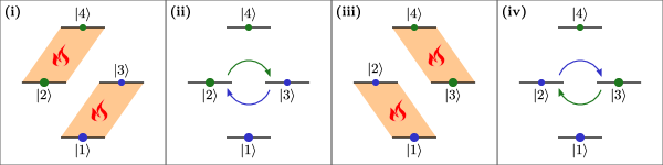
Figure 1: Periodically driven quantum four-level system without a unique limit cycle. The states $|1\rangle$ through $|4\rangle$ are indicated by horizontal lines in the diagrams; the filled circles on the lines indicate the level populations at the beginning of each step. We consider a cyclic four-step protocol: 1. The populations of the pairs of states $(|1\rangle,|3\rangle)$ and $(|2\rangle,|4\rangle)$ thermalize separately. That is, the time evolution during this step follows (1) with constant Lindblad generator $\hat{L}_{t}=\hat{L}$. The generator contains four dissipative terms with the Lindblad operators $|1\rangle\!\langle 3|$, $|2\rangle\!\langle 4|$, and their adjoints. 2. The populations of the states $|2\rangle$ and $|3\rangle$ are swapped unitarily. 3. The populations of the pairs $(|1\rangle,|2\rangle)$ and $(|3\rangle,|4\rangle)$ of states thermalize separately. 4. The populations of the states $|2\rangle$ and $|3\rangle$ are swapped unitarily. The ratio between the populations marked in green and the populations marked in blue is determined by the initial conditions and remains unaltered over one period. Hence, the long time state cannot be unique.

Finally, it is a natural question to ask whether the conditions of Theorem 2 could be weakened. A weaker condition might, for example, only require that $\bigcup_{t\in[0,T]}\mathcal{A}_{t}$ is irreducible, i.e., that the dissipative dynamics connects all subspaces over the course of one driving period. A simple counterexample, illustrated in Figure 1, shows, however, that this condition is not sufficient for the limit cycle to be unique. Hence, potential generalizations of Theorem 2 would most likely require a closer analysis of the interplay between the unitary and the dissipative parts of the GKSL equation. It remains a challenge for future investigations to settle the question whether such extensions can be formulated in terms of simple algebraic conditions.

References

- Breuer and Petruccione [2002] H.-P. Breuer and F. Petruccione, The Theory of Open Quantum Systems (Oxford University Press, 2002).
- Gorini et al. [1976] V. Gorini, A. Kossakowski, and E. C. G. Sudarshan, Completely positive dynamical semigroups of N-level systems, J. Math. Phys. 17, 821 (1976).
- Lindblad [1976] G. Lindblad, On the generators of quantum dynamical semigroups, Commun. Math. Phys. 48, 119 (1976).
- Chruściński and Kossakowski [2012] D. Chruściński and A. Kossakowski, Markovianity criteria for quantum evolution, J. Phys. B 45, 154002 (2012).
- Rivas and Huelga [2012] Á. Rivas and S. F. Huelga, Open Quantum Systems. An Introduction, SpringerBriefs in Physics (Springer, 2012).
- Scully and Zubairy [1997] M. O. Scully and M. S. Zubairy, Quantum Optics (Cambridge University Press, 1997).
- Nielsen and Chuang [2000] M. A. Nielsen and I. L. Chuang, Quantum Computation and Quantum Information (Cambridge University Press, 2000).
- Goold et al. [2016] J. Goold, M. Huber, A. Riera, L. del Rio, and P. Skrzypczyk, The role of quantum information in thermodynamics—a topical review, J. Phys. A 49, 143001 (2016).
- Kosloff [2013] R. Kosloff, Quantum Thermodynamics: A Dynamical Viewpoint, Entropy 15, 2100 (2013).
- Vinjanampathy and Anders [2016] S. Vinjanampathy and J. Anders, Quantum thermodynamics, Contemp. Phys. 57, 545 (2016).
- Benenti et al. [2017] G. Benenti, G. Casati, K. Saito, and R. S. Whitney, Fundamental aspects of steady-state conversion of heat to work at the nanoscale, Phys. Rep. 694, 1 (2017).
- Pekola [2015] J. P. Pekola, Towards quantum thermodynamics in electronic circuits, Nat. Phys. 11, 118 (2015).
- Gorini et al. [1978] V. Gorini, A. Frigerio, M. Verri, A. Kossakowski, and E. C. G. Sudarshan, Properties of quantum Markovian master equations, Rep. Math. Phys. 13, 149 (1978).
- Spohn [1978] H. Spohn, Entropy production for quantum dynamical semigroups, J. Math. Phys. 19, 1227 (1978).
- Alicki and Fannes [1987] R. Alicki and M. Fannes, Dilations of quantum dynamical semigroups with classical Brownian motion, Commun.Math. Phys. 108, 353 (1987).
- Alicki and Lendi [2007] R. Alicki and K. Lendi, Quantum Dynamical Semigroups and Applications, Lecture Notes in Physics, Vol. 717 (Springer, Berlin, Heidelberg, 2007).
- Schirmer and Wang [2010] S. G. Schirmer and X. Wang, Stabilizing open quantum systems by Markovian reservoir engineering, Phys. Rev. A 81, 062306 (2010).
- Albert et al. [2016] V. V. Albert, B. Bradlyn, M. Fraas, and L. Jiang, Geometry and Response of Lindbladians, Phys. Rev. X 6, 041031 (2016).
- Breuer et al. [2016] H.-P. Breuer, E.-M. Laine, J. Piilo, and B. Vacchini, Non-Markovian dynamics in open quantum systems, Rev. Mod. Phys. 88, 021002 (2016).
- Spohn [1977] H. Spohn, An algebraic condition for the approach to equilibrium of an open N-level system, Lett. Math. Phys 2, 33 (1977).
- Brandner and Seifert [2016] K. Brandner and U. Seifert, Periodic thermodynamics of open quantum systems, Phys. Rev. E 93, 062134 (2016).
- Gambetta et al. [2019] F. M. Gambetta, F. Carollo, A. Lazarides, I. Lesanovsky, and J. P. Garrahan, Classical Stochastic Discrete Time Crystals, arXiv:1905.08826 [cond-mat.stat-mech] (2019).
- Reed and Simon [1981] M. Reed and B. Simon, Functional Analysis, Methods of Modern Mathematical Physics No. 1 (Academic Press, 1981).
- Feldmann and Kosloff [2004] T. Feldmann and R. Kosloff, Characteristics of the limit cycle of a reciprocating quantum heat engine, Phys. Rev. E 70, 046110 (2004).
- Kosloff and Rezek [2017] R. Kosloff and Y. Rezek, The Quantum Harmonic Otto Cycle, Entropy 19, 136 (2017).
- Scopa et al. [2018] S. Scopa, G. T. Landi, and D. Karevski, Lindblad-Floquet description of finite-time quantum heat engines, Phys. Rev. A 97, 062121 (2018).