Lectures on the Error Analysis of Interpolation
on Simplicial Triangulations without
the Shape Regularity Assumption
Part 1: Lagrange Interpolation on Triangles

Abstract: In the error analysis of finite element methods, the shape regularity assumption on triangulations is typically imposed to obtain a priori error estimations. In practical computations, however, very “thin” or “degenerated” elements that violate the shape regularity assumption may appear when we use adaptive mesh refinement. In this survey, we attempt to establish an error analysis approach without the shape regularity assumption on triangulations.

We have presented several papers on the error analysis of finite element methods on non-shape regular triangulations. The main points in these papers are that, in the error estimates of finite element methods, the circumradius of the triangles is one of the most important factors.

The purpose of this survey is to provide a simple and plain explanation of the results to researchers and, in particular, graduate students who are interested in the subject. Therefore, this survey is not intended to be a research paper. We hope that, in the near future, it will be merged into a textbook on the mathematical theory of the finite element methods.

1 Introduction: Lagrange interpolation on triangles

Lagrange interpolation on triangles and the associated error estimates are important subjects in numerical analysis. In particular, they are crucial in the error analysis of finite element methods. Throughout this survey, $K\subset\mathbb{R}^{2}$ denotes a triangle with vertices $\mathbf{x}_{i}$, $i=1,2,3$. In this survey, we always assume that triangles are closed sets. Let $\lambda_{i}$ be the barycentric coordinates of $K$ with respect to $\mathbf{x}_{i}$. By definition, $0\leq\lambda_{i}\leq 1$, $\sum_{i=1}^{3}\lambda_{i}=1$. Let $\mathbb{N}_{0}$ be the set of nonnegative integers, and $\gamma=(a_{1},a_{2},a_{3})\in\mathbb{N}_{0}^{3}$ be a multi-index. Let $k$ be a positive integer. If $|\gamma|:=\sum_{i=1}^{d+1}a_{i}=k$, then ${\gamma}/{k}:=\left(a_{1}/k,a_{2}/k,a_{3}/k\right)$ can be regarded as a barycentric coordinate in $K$. The set $\Sigma^{k}(K)$ of points on $K$ is defined as

$$\Sigma^{k}(K):=\left\{\frac{\gamma}{k}\in K\Bigm{|}|\gamma|=k,\;\gamma\in\mathbb{N}_{0}^{3}\right\}.$$ (1)

Figure 1: Set $\Sigma^{k}(K)$, $k=1$, $k=2$, $k=3$.

Let $\mathcal{P}_{k}(K)$ be a set of polynomials defined on $K$ whose degree is at most $k$. For a continuous function $v\in C^{0}(K)$, the $k$th-order Lagrange interpolation $\mathcal{I}_{K}^{k}v\in\mathcal{P}_{k}(K)$ is defined as

$$v(\mathbf{x})=(\mathcal{I}_{K}^{k}v)(\mathbf{x}),\qquad\forall\mathbf{x}\in\Sigma^{k}(K).$$

To enable the error analysis of Lagrange interpolation, we typically introduce the following condition [8, 6, 10]. Let $h_{K}:=\mathrm{diam}K$ and $\rho_{K}$ be the diameter of its inscribed circle. Suppose that $X$ is a set of (possibly infinitely many) triangles.

Assumption 1 (Shape regularity)

The set $X$ is called shape regular if there exists a constant $\sigma>0$ such that $\displaystyle\frac{h_{K}}{\rho_{K}}\leq\sigma,\qquad\forall K\in X.$

The maximum of the ratio $h_{K}/\rho_{K}$ in $X$ is called its chunkiness parameter [6]. The shape regularity condition is sometimes also called the inscribed ball condition. For more information on the conditions equivalent to shape regularity, see [9].

Let $\widehat{K}$ be a reference element. The triangle with vertices $(0,0)^{\top}$, $(1,0)^{\top}$, and $(0,1)^{\top}$ is typically taken as the reference triangle $\widehat{K}$. Let $\varphi(\mathbf{x})=A\mathbf{x}+\mathbf{b}$ be an affine transformation that maps $\widehat{K}$ to $K$, where $A$ is a $2\times 2$ regular matrix and $\mathbf{b}\in\mathbb{R}^{2}$.

Error analysis is first performed on the reference element $\widehat{K}$. Then, the “pull back” with $v\circ\varphi$ is used to transfer the result obtained on $\widehat{K}$ to the “physical element” $K$.

Let $\|A\|$ denote the matrix norm of $A$ associated with the Euclidean norm of $\mathbb{R}^{2}$, and let $1\leq p\leq\infty$. The function $v\in W^{k+1,p}(K)$ is pulled back by $\varphi$ as $\hat{v}:=v\circ\varphi$. Let $k$ and $m$ be integers such that $k\geq 1$ and $0\leq m\leq k$. The following theorem is standard.

Theorem 2 ([8], Theorem 3.1.4)

Let $\sigma>0$ be a constant. If $h_{K}/\rho_{K}\leq\sigma$, then there exists a constant $C=C(\widehat{K},p,k,m)$ independent of $K$ such that, for $v\in W^{k+1,p}(K)$, $\displaystyle|v-\mathcal{I}_{K}^{k}v|_{m,p,K}$ $\displaystyle\leq C\|A\|^{k+1}\|A^{-1}\|^{m}|v|_{k+1,p,K}$ $\displaystyle\leq C\frac{h_{K}^{k+1}}{\rho_{K}^{m}}|v|_{k+1,p,K}\leq(C\sigma^{m})h_{K}^{k+1-m}|v|_{k+1,p,K}.$ (2)

To derive the second inequality in (2), we use the following lemma.

Lemma 3 ([8], Theorem 3.1.3)

We have $\|A\|\leq h_{K}\rho_{\widehat{K}}^{-1}$, $\|A^{-1}\|\leq h_{\widehat{K}}\rho_{K}^{-1}$.

Let $K$ be an arbitrary triangle, and $h_{K}\geq\alpha\geq\beta>0$ be the lengths of its three edges. Note that $h_{K}/2<\alpha\leq h_{K}$. Using translation, rotation, and mirror imaging, $K$ is transformed into a triangle with vertices $\mathbf{x}_{1}=(0,0)^{\top}$, $\mathbf{x}_{2}=(\alpha,0)^{\top}$, and $\mathbf{x}_{3}=(\beta s,\beta t)^{\top}$, where $s=\cos\theta$, $t=\sin\theta$, and $0<\theta<\pi$ is the inner angle of $K$ at $\mathbf{x}_{1}$. This triangle is called the standard position of $K$. By the law of cosines,

$$h_{K}^{2}=\alpha^{2}+\beta^{2}-2\alpha\beta\cos\theta\quad\text{ and }\quad\cos\theta=\frac{\beta}{2\alpha}+\frac{\alpha^{2}-h_{K}^{2}}{2\alpha\beta}\leq\frac{\beta}{2\alpha}\leq\frac{1}{2}.$$

Hence, $\pi/3\leq\theta<\pi$.

Figure 2: General triangle $K$ in the standard position. The vertices are $\mathbf{x}_{1}=(0,0)^{\top}$, $\mathbf{x}_{2}=(\alpha,0)^{\top}$, and $\mathbf{x}_{3}=(\beta s,\beta t)^{\top}$, where $s^{2}+t^{2}=1$, $t>0$. We assume that $0<\beta\leq\alpha\leq h_{K}$.

These assumptions imply that the affine transformation $\varphi$ can be written as $\varphi(\mathbf{x})=A\mathbf{x}$ with the matrix

$$A=\begin{pmatrix}\alpha&\beta s\\ 0&\beta t\end{pmatrix}.$$ (3)

We set $t=\sin\theta=1$, for example (i.e., $K$ is a right triangle). Then, $s=0$, $\|A\|=\alpha$, $\|A^{-1}\|=1/\beta$, and the inequalities in (24) can be rearranged as

$$|v-\mathcal{I}_{K}^{k}v|_{m,p,K}\leq C\frac{\alpha^{k+1}}{\beta^{m}}|v|_{k+1,p,K}\leq C\left(\frac{\alpha}{\beta}\right)^{m}h_{K}^{k+1-m}|v|_{k+1,p,K}.$$ (4)

Thus, we might consider that the ratio $\alpha/\beta$ should not be too large, or $K$ should not be too “flat.” This consideration is expressed as the minimum angle condition (Zlámal [28], Ženíšek [27]), which is equivalent to the shape regularity condition for triangles.

Theorem 4 (Minimum angle condition)

Let $\theta_{0}$, $(0<\theta_{0}\leq\pi/3)$ be a constant. If any angle $\theta$ of $K$ satisfies $\theta\geq\theta_{0}$ and $h_{K}\leq 1$, then there exists a constant $C=C(\theta_{0})$ independent of $h_{K}$ such that $\displaystyle|v-\mathcal{I}_{K}^{1}v|_{1,2,K}\leq Ch_{K}|v|_{2,2,K},\qquad\forall v\in H^{2}(K).$

However, the minimum angle condition and shape regularity are not necessarily needed to obtain an error estimate. The following condition is well known (Babuška–Aziz [4]).

Theorem 5 (Maximum angle condition)

Let $\theta_{1}$, $(\pi/3\leq\theta_{1}<\pi)$ be a constant. If any angle $\theta$ of $K$ satisfies $\theta\leq\theta_{1}$ and $h_{K}\leq 1$, then there exists a constant $C=C(\theta_{1})$ that is independent of $h_{K}$ such that $$|v-\mathcal{I}_{K}^{1}v|_{1,2,K}\leq Ch_{K}|v|_{2,2,K},\qquad\forall v\in H^{2}(K).$$ (5)

Křížek [19] introduced the semiregularity condition, which is equivalent to the maximum angle condition (see Remark below). Let $R_{K}$ be the circumradius of $K$.

Theorem 6 (Semiregularity condition)

Let $p>1$ and $\sigma>0$ be a constant. If $R_{K}/h_{K}\leq\sigma$ and $h_{K}\leq 1$, then there exists a constant $C=C(\sigma)$ that is independent of $h_{K}$ such that $\displaystyle|v-\mathcal{I}_{K}^{1}v|_{1,p,K}\leq Ch_{K}|v|_{2,p,K},\qquad\forall v\in W^{2,p}(K).$

We mention a few more known results. Jamet [13] presented the following results.

Theorem 7

Let $1\leq p\leq\infty$. Let $m\geq 0$, $k\geq 1$ be integers such that $k+1-m>2/p$ $(1<p\leq\infty)$ or $k-m\geq 1$ $(p=1)$. Then, the following estimate holds: $$|v-\mathcal{I}_{K}^{k}v|_{m,p,K}\leq C\frac{h_{K}^{k+1-m}}{\cos^{m}\theta_{K}/2}|v|_{k+1,p,K},\quad\forall v\in W^{k+1,p}(K),$$ (6) where $\theta_{K}$ is the maximum angle of $K$, and $C$ depends only on $k$ and $p$.

Remark: (1) In Theorem 7, the restriction on $p$ comes from the Sobolev imbedding theorem. Note that in [13, Théorème 3.1] the case $p=1$ is not mentioned explicitly but clearly holds for triangles (see Section 2.5). For the case of the maximum angle condition, we set $k=m=1$ and find that Jamet’s result (Theorem 7) does not imply the estimation (5) because the case $p=2$ is excluded.

(2) Let an arbitrary triangle $K$ be in its standard position (Figure 2). Then $\theta$ is the maximum internal angle of $K$, and

$$\frac{R_{K}}{h_{K}}=\frac{1}{2\sin\theta},\qquad\frac{\pi}{3}\leq\theta<\pi$$ (7)

by the law of sines. Thus, the dimensionless quantity $R_{K}/h_{K}$ represents the maximum internal angle of $K$, and the boundedness of $R_{K}/h_{K}$, which is the semiregularity of $K$, is equivalent to the maximum angle condition $\theta\leq\theta_{1}<\pi$ with a fixed constant $\theta_{1}$. $\square$

For further results of the error estimations on “skinny elements”, see the monograph by Apel [2].

Recently, Kobayashi, one of the authors, obtained the following epoch-making result [14]. Let $A$, $B$, and $C$ be the lengths of the three edges of $K$ and $S$ be the area of $K$.

Theorem 8 (Kobayashi’s formula)

We define the constant $C(K)$ as $\displaystyle C(K):=\sqrt{\frac{A^{2}B^{2}C^{2}}{16S^{2}}-\frac{A^{2}+B^{2}+C^{2}}{30}-\frac{S^{2}}{5}\left(\frac{1}{A^{2}}+\frac{1}{B^{2}}+\frac{1}{C^{2}}\right)}.$ Then the following holds: $\displaystyle|v-\mathcal{I}_{K}^{1}v|_{1,2,K}\leq C(K)|v|_{2,2,K},\qquad\forall v\in H^{2}(K).$

Recall that $R_{K}$ is the circumradius of $K$ and is written as

$$R_{K}=\frac{ABC}{4S}.$$ (8)

Then, we immediately realize that $C(K)<R_{K}$ and obtain a corollary of Kobayashi’s formula.

Corollary 9

For any triangle $K\subset\mathbb{R}^{2}$, the following estimate holds: $$|v-\mathcal{I}_{K}^{1}v|_{1,2,K}\leq R_{K}|v|_{2,2,K},\qquad\forall v\in H^{2}(K).$$ (9)

This corollary demonstrates that even if the minimum angle is very small or the maximum angle is very close to $\pi$, the error $|v-\mathcal{I}_{K}^{1}v|_{1,K}$ converges to $0$ if $R_{K}$ converges to $0$. We consider the isosceles triangle $K$ shown in Figure 3 (left). Using (8), we realize that $R_{K}=h^{\alpha}/2+h^{2-\alpha}/8=\mathcal{O}(h^{2-\alpha})$ ($\alpha\geq 1$, $h\leq 1$). Thus, if $\alpha<2$, $R_{K}\to 0$ as $h\to 0$.

As another example, let $\alpha$, $\beta\in\mathbb{R}$ satisfy $1<\alpha<\beta<1+\alpha$. We consider the triangle $K$ whose vertices are $(0,0)^{\top}$, $(h,0)^{\top}$, and $(h^{\alpha},h^{\beta})^{\top}$ (Figure 3 (right)). With (8), it is straightforward to see

$$R_{K} =\frac{h\left(h^{2\alpha}+h^{2\beta}\right)^{1/2}\left((h^{\alpha}-h)^{2}+h^{2\beta}\right)^{1/2}}{2h^{1+\beta}}$$ (10)

$$=\frac{h^{1+\alpha}}{2h^{\beta}}\left(1+h^{2\beta-2\alpha}\right)^{1/2}\left(1+h^{2\alpha-2}-2h^{\alpha-1}+h^{2\beta-2}\right)^{1/2}=\mathcal{O}(h^{1+\alpha-\beta}),$$ (11)

$$\rho_{K} =\frac{h^{1+\beta}}{h+\left(h^{2\alpha}+h^{2\beta}\right)^{1/2}+\left((h^{\alpha}-h)^{2}+h^{2\beta}\right)^{1/2}},\quad\frac{h^{\beta}}{3}<\rho_{K}<h^{\beta}.$$ (12)

Hence, if $h\to 0$, the convergence rates that (2) and (9) yield are $\mathcal{O}(h^{2-\beta})$ and $\mathcal{O}(h^{1+\alpha-\beta})$, respectively. Therefore, (9) obtains a better convergence rate than (2). Moreover, if $\beta\geq 2$, (2) does not yield convergence whereas (9) does. Note that, when $h\to 0$, the maximum angles of $K$ approach to $\pi$ in both cases.

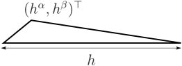
Figure 3: Examples of triangles that violate the maximum angle condition but satisfy $R_{K}\to 0$ as $h\to 0$.

Although Kobayashi’s formula is remarkable, its proof is long and needs validated numerical computation. We began this research to provide a “paper-and-pencil” proof of (9), and recently reported an error estimation in terms of the circumradius of a triangle [15, 17, 18].

Theorem 10 (Circumradius estimates)

Let $K$ be an arbitrary triangle. Then, for the $k$th-order Lagrange interpolation $\mathcal{I}_{K}^{k}$ on $K$, the estimation $$|v-\mathcal{I}_{K}^{k}v|_{m,p,K}\leq C\left(\frac{R_{K}}{h_{K}}\right)^{m}h_{K}^{k+1-m}|v|_{k+1,p,K}=CR_{K}^{m}h_{K}^{k+1-2m}|v|_{k+1,p,K}$$ (13) holds for any $v\in W^{k+1,p}(K)$, where the constant $C=C(k,m,p)$ is independent of the geometry of $K$.

We recall that a general triangle $K$ may be written using the settings in Figure 2. The essence of the proof of Theorem 10 is that the matrix $A$ in (3) is decomposed as

$$A=\widetilde{A}D_{\alpha\beta},\qquad\widetilde{A}:=\begin{pmatrix}1&s\\ 0&t\end{pmatrix},\quad D_{\alpha\beta}:=\begin{pmatrix}\alpha&0\\ 0&\beta\end{pmatrix}.$$

With this decomposition, the estimate (2) is rearranged as

$$|v-\mathcal{I}_{K}^{k}v|_{m,p,K} \leq C\|\widetilde{A}\|^{k+1}\|\widetilde{A}^{-1}\|^{m}\|D_{\alpha\beta}\|^{k+1}\|D_{\alpha\beta}^{-1}\|^{m}|v|_{k+1,p,K}.$$ (14)

As indicated by us [18] and Babuška–Aziz [4], the linear transformation by $D_{\alpha\beta}$ does not reduce the approximation property of Lagrange interpolation, and only $\widetilde{A}$ could make it “bad.” This means that the term

$$\|D_{\alpha\beta}\|^{k+1}\|D_{\alpha\beta}^{-1}\|^{m}=\frac{(\max\{\alpha,\beta\})^{k+1}}{(\min\{\alpha,\beta\})^{m}}\quad\text{may be replaced with}\;C_{1}h_{K}^{k+1-m}.$$

Furthermore, $\|\widetilde{A}\|$ and $\|\widetilde{A}^{-1}\|$ (the maximum singular values of $\widetilde{A}$ and $\widetilde{A}^{-1}$) are bounded using the circumradius $R_{K}$ and $h_{K}$ as

$$\|\widetilde{A}\|^{k+1}\|\widetilde{A}^{-1}\|^{m}\leq C_{2}\left(\frac{R_{K}}{h_{K}}\right)^{m},\quad\frac{R_{K}}{h_{K}}=\frac{1}{2\sin\theta},$$

where $\theta$ is the maximum internal angle of $K$ (see Figure 2 and (7)). We emphasize that the constants $C_{i}$ $(i=1,2)$ only depend on $k$, $m$, and $p$. Note that, by setting $t=1$ and $\beta=\alpha^{2}$ in (2) (and (4)), we realize that, regardless of how much we try to analyze $\|A\|^{k+1}\|A^{-1}\|^{m}$, we cannot prove Theorem 10. In the sequel of this survey, we will explain the proof of Theorem 10 in detail.

2 Preliminaries

2.1 Notation

Let $n\geq 1$ be a positive integer and $\mathbb{R}^{n}$ be $n$-dimensional Euclidean space. We denote the Euclidean norm of $\mathbf{x}\in\mathbb{R}^{n}$ by $|\mathbf{x}|$. Let $\mathbb{R}^{n*}:=\{l:\mathbb{R}^{n}\to\mathbb{R}:l\text{ is linear}\}$ be the dual space of $\mathbb{R}^{n}$. We always regard $\mathbf{x}\in\mathbb{R}^{n}$ as a column vector and $\mathbf{a}\in\mathbb{R}^{n*}$ as a row vector. For a matrix $A$ and $\mathbf{x}\in\mathbb{R}^{n}$, $A^{\top}$ and $\mathbf{x}^{\top}$ denote their transpositions. For matrices $A=(a_{ij})_{i,j=1,\cdots,n}$ and $B=(b_{ij})_{i,j=1,\cdots,n}$, their Kronecker product $A\otimes B$ is an $n^{2}\times n^{2}$ matrix defined as

$$A\otimes B:=\begin{pmatrix}a_{11}B&\cdots&a_{1n}B\\ \vdots&&\vdots\\ a_{n1}B&\cdots&a_{nn}B\\ \end{pmatrix}.$$

For matrices $A_{i}$, $i=1,\cdots,k$, the Kronecker product $A_{1}\otimes\cdots\otimes A_{k}$ is defined recursively.

For a differentiable function $f$ with $n$ variables, its gradient $\nabla f=\mathrm{grad}f\in\mathbb{R}^{n*}$ is the row vector defined as

$$\nabla f=\nabla_{\mathbf{x}}f:=\left(\frac{\partial f}{\partial x_{1}},\cdots,\frac{\partial f}{\partial x_{n}}\right),\qquad\mathbf{x}:=(x_{1},\cdots,x_{n})^{\top}.$$

Let $\mathbb{N}_{0}$ be the set of nonnegative integers. For $\delta=(\delta_{1},...,\delta_{n})\in(\mathbb{N}_{0})^{n}$, the multi-index $\partial^{\delta}$ of partial differentiation (in the sense of distribution) is defined by

$$\partial^{\delta}=\partial_{\mathbf{x}}^{\delta}:=\frac{\partial^{|\delta|}\ }{\partial x_{1}^{\delta_{1}}\cdots\partial x_{n}^{\delta_{n}}},\qquad|\delta|:=\delta_{1}+\cdots+\delta_{n}.$$

For two multi-indices $\eta=(\eta_{1},\cdots,\eta_{n})$, $\delta=(\delta_{1},\cdots,\delta_{n})$, $\eta\leq\delta$ means that $\eta_{i}\leq\delta_{i}$ $(i=1,\cdots,n)$. Additionally, $\delta\cdot\eta$ and $\delta!$ are defined as $\delta\cdot\eta:=\eta_{1}\delta_{1}+\cdots+\eta_{n}\delta_{n}$ and $\delta!:=\delta_{1}!\cdots\delta_{n}!$, respectively.

Let $\Omega\subset\mathbb{R}^{n}$ be a (bounded) domain. The usual Lebesgue space is denoted by $L^{p}(\Omega)$ for $1\leq p\leq\infty$. For a positive integer $k$, the Sobolev space $W^{k,p}(\Omega)$ is defined by $\displaystyle W^{k,p}(\Omega):=\left\{v\in L^{p}(\Omega)\,|\,\partial^{\delta}v\in L^{p}(\Omega),\,|\delta|\leq k\right\}$. For $1\leq p<\infty$, the norm and semi-norm of $W^{k,p}(\Omega)$ are defined as

$$|v|_{k,p,\Omega}:=\biggl{(}\sum_{|\delta|=k}|\partial^{\delta}v|_{0,p,\Omega}^{p}\biggr{)}^{1/p},\quad\|v\|_{k,p,\Omega}:=\biggl{(}\sum_{0\leq m\leq k}|v|_{m,p,\Omega}^{p}\biggr{)}^{1/p},$$

and $\displaystyle|v|_{k,\infty,\Omega}:=\max_{|\delta|=k}\left\{\mathrm{ess}\sup_{\mathbf{x}\in\Omega}|\partial^{\delta}v(\mathbf{x})|\right\}$, $\displaystyle\|v\|_{k,\infty,\Omega}:=\max_{0\leq m\leq k}\left\{|v|_{m,\infty,\Omega}\right\}$.

2.2 Preliminaries from matrix analysis

We introduce some facts from the theory of matrix analysis. For their proofs, refer to textbooks on matrix analysis such as [12] and [26].

Let $n\geq 2$ be an integer and $A$ be an $n\times n$ regular matrix. Note that $A^{\top}A$ is symmetric positive-definite and has $n$ positive eigenvalues $0<\mu_{1}\leq\cdots\leq\mu_{n}$. The square roots of $\mu_{i}$ are called the singular values of $A$. Let $\mu_{m}:=\mu_{1}$ and $\mu_{M}:=\mu_{n}$ be the minimum and maximum eigenvalues. Then,

$$\mu_{m}|\mathbf{x}|^{2}\leq|A\mathbf{x}|^{2}\leq\mu_{M}|\mathbf{x}|^{2},\quad\mu_{M}^{-1}|\mathbf{x}|^{2}\leq|A^{-1}\mathbf{x}|^{2}\leq\mu_{m}^{-1}|\mathbf{x}|^{2},\quad\forall\mathbf{x}\in\mathbb{R}^{n}.$$

For $A$, the matrix norm $\|A\|$ with respect to the Euclidean norm is defined by

$$\|A\|:=\sup_{\mathbf{x}\in\mathbb{R}^{n}}\frac{|A\mathbf{x}|}{|\mathbf{x}|}.$$

From these definitions, we realize that $\|A\|=\mu_{M}^{1/2}$ and $\|A^{-1}\|=\mu_{m}^{-1/2}$.

For the Kronecker product of matrices, we have the following lemma whose proof is straightforward (see the textbooks mentioned above).

Lemma 11

Let $A$, $B$, $C$, and $D$ be $n\times n$ matrices. Then, the following equations hold: $\displaystyle(A\otimes B)(C\otimes D)=(AC\otimes BD),\qquad(A\otimes B)^{\top}=A^{\top}\otimes B^{\top}.$ Furthermore, if $A$ and $B$ have eigenvalues $\lambda_{i}$ and $\mu_{j}$, $i,j=1,\cdots,n$, respectively, then $\lambda_{i}\mu_{j}$ are eigenvalues of $A\otimes B$.

Exercise: Prove Lemma 11.

From Lemma 11, we realize that the minimum and maximum eigenvalues of $(A^{\top}A)\otimes(A^{\top}A)=(A\otimes A)^{\top}(A\otimes A)$ are $0<\mu_{m}^{2}\leq\mu_{M}^{2}$. Hence, for any $\mathbf{w}\in\mathbb{R}^{n^{2}}$,

$$\mu_{m}^{2}|\mathbf{w}|^{2}\leq|(A\otimes A)\mathbf{w}|^{2} \leq\mu_{M}^{2}|\mathbf{w}|^{2},\quad\mu_{M}^{-2}|\mathbf{w}|^{2}\leq|(A^{-1}\otimes A^{-1})\mathbf{w}|^{2}\leq\mu_{m}^{-2}|\mathbf{w}|^{2}.$$

The above facts can be extended straightforwardly to the case of the higher-order Kronecker product $A\otimes...\otimes A$. For $A\otimes...\otimes A$, $A^{-1}\otimes...\otimes A^{-1}$ (the $k$th Kronecker products), and we have, for $\mathbf{w}\in\mathbb{R}^{n^{k}}$,

$$\mu_{m}^{k}|\mathbf{w}|^{2} \leq|(A\otimes...\otimes A)\mathbf{w}|^{2}\leq\mu_{M}^{k}|\mathbf{w}|^{2},$$

$$\mu_{M}^{-k}|\mathbf{w}|^{2} \leq|(A^{-1}\otimes...\otimes A^{-1})\mathbf{w}|^{2}\leq\mu_{m}^{-k}|\mathbf{w}|^{2}.$$

These inequalities imply that

$$\|A\otimes...\otimes A\|=\|A\|^{k},\qquad\|A^{-1}\otimes...\otimes A^{-1}\|=\|A^{-1}\|^{k}.$$

2.3 Useful inequalities

For $N$ positive real numbers $U_{1},...,U_{N}$, the following inequalities hold:

$$\sum_{k=1}^{N}U_{k}^{p}\leq N^{\tau(p)}\left(\sum_{k=1}^{N}U_{k}^{2}\right)^{p/2},\quad\tau(p):=\begin{cases}1-p/2,&1\leq p\leq 2\\ 0,&2\leq p<\infty\end{cases},$$ (15)

$$\left(\sum_{k=1}^{N}U_{k}^{2}\right)^{p/2}\leq N^{\gamma(p)}\sum_{k=1}^{N}U_{k}^{p},\quad\gamma(p):=\begin{cases}0,&1\leq p\leq 2\\ p/2-1,&2\leq p<\infty\end{cases}.$$ (16)

Exercise: Prove the inequalities (15) and (16).

2.4 The affine transformation defined by a regular matrix

Let $A$ be an $n\times n$ matrix with det$A>0$. We consider the affine transformation $\varphi(\mathbf{x})$ defined by $\mathbf{y}=\varphi(\mathbf{x}):=A\mathbf{x}+\mathbf{b}$ for $\mathbf{x}=(x_{1},\cdots,x_{n})^{\top}$, $\mathbf{y}=(y_{1},\cdots,y_{n})^{\top}$ with $\mathbf{b}\in\mathbb{R}^{n}$. Suppose that a reference region $\widehat{\Omega}\subset\mathbb{R}^{n}$ is transformed to a domain $\Omega$ by $\varphi$; $\Omega:=\varphi(\widehat{\Omega})$. Then, a function $v(\mathbf{y})$ defined on $\Omega$ is pulled-back to the function $\hat{v}(\mathbf{x})$ on $\widehat{\Omega}$ as $\hat{v}(\mathbf{x}):=v(\varphi(\mathbf{x}))=v(\mathbf{y})$. Then, we have $\nabla_{\mathbf{x}}\hat{v}=(\nabla_{\mathbf{y}}v)A$, $\nabla_{\mathbf{y}}v=(\nabla_{\mathbf{x}}\hat{v})A^{-1}$, and $|\nabla_{\mathbf{y}}v|^{2}=|(\nabla_{\mathbf{x}}\hat{v})A^{-1}|^{2}=(\nabla_{\mathbf{x}}\hat{v})A^{-1}A^{-\top}(\nabla_{\mathbf{x}}\hat{v})^{\top}$.

The Kronecker product $\nabla\otimes\nabla$ of the gradient $\nabla$ is defined by

$$\nabla\otimes\nabla:=\left(\frac{\partial\ }{\partial x_{1}}\nabla,...,\frac{\partial\ }{\partial x_{n}}\nabla\right)=\left(\frac{\partial^{2}\ }{\partial x_{1}^{2}},\frac{\partial^{2}\ }{\partial x_{1}\partial x_{2}},...,\frac{\partial^{2}\ }{\partial x_{n-1}\partial x_{n}},\frac{\partial^{2}\ }{\partial x_{n}^{2}}\right).$$

We regard $\nabla\otimes\nabla$ to be a row vector. From this definition, it follows that

$$\sum_{|\delta|=2}(\partial^{\delta}v)^{2}=\sum_{i,j=1}^{n}\left(\frac{\partial^{2}v}{\partial x_{i}\partial x_{j}}\right)^{2}=|(\nabla\otimes\nabla)v|^{2}$$

and $(\nabla_{\mathbf{x}}\otimes\nabla_{\mathbf{x}})\hat{v}=\left((\nabla_{\mathbf{y}}\otimes\nabla_{\mathbf{y}})v\right)(A\otimes A)$, $(\nabla_{\mathbf{y}}\otimes\nabla_{\mathbf{y}})v=\left((\nabla_{\mathbf{x}}\otimes\nabla_{\mathbf{x}})\hat{v}\right)(A^{-1}\otimes A^{-1})$. Thus, we have $\|A\|^{-2}|\nabla_{\mathbf{x}}\hat{v}|^{2}\leq|\nabla_{\mathbf{y}}v|^{2}\leq\|A^{-1}\|^{2}|\nabla_{\mathbf{x}}\hat{v}|^{2}$ and

$$\sum_{|\delta|=2}(\partial_{\mathbf{y}}v)^{2} =|(\nabla_{\mathbf{y}}\otimes\nabla_{\mathbf{y}})v|^{2}$$

$$=\left((\nabla_{\mathbf{x}}\otimes\nabla_{\mathbf{x}})\hat{v}\right)(A^{-1}\otimes A^{-1})(A^{-1}\otimes A^{-1})^{\top}\left((\nabla_{\mathbf{x}}\otimes\nabla_{\mathbf{x}})\hat{v}\right)^{\top}$$

$$=\left((\nabla_{\mathbf{x}}\otimes\nabla_{\mathbf{x}})\hat{v}\right)(A^{-1}A^{-\top}\otimes A^{-1}A^{-\top})\left((\nabla_{\mathbf{x}}\otimes\nabla_{\mathbf{x}})\hat{v}\right)^{\top},$$

$$\|A\|^{-2}\sum_{|\delta|=2}(\partial_{\mathbf{x}}^{\delta}\hat{v})^{2} \leq\sum_{|\delta|=2}(\partial_{\mathbf{y}}^{\delta}v)^{2}\leq\|A^{-1}\|^{2}\sum_{|\delta|=2}(\partial_{\mathbf{x}}^{\delta}\hat{v})^{2}.$$

The above inequalities can be easily extended to higher-order derivatives, and we obtain the following inequalities: for $k\geq 1$,

$$\|A\|^{-2k}\sum_{|\delta|=k}(\partial_{\mathbf{x}}^{\delta}\hat{v})^{2}\leq\sum_{|\delta|=k}(\partial_{\mathbf{y}}^{\delta}v)^{2}\leq\|A^{-1}\|^{2k}\sum_{|\delta|=k}(\partial_{\mathbf{x}}^{\delta}\hat{v})^{2},$$

$$|\!\det{A}|^{1/2}\|A\|^{-k}|\hat{v}|_{k,2,\widehat{\Omega}}\leq|v|_{k,2,\Omega}\leq|\!\det{A}|^{1/2}\|A^{-1}\|^{k}|\hat{v}|_{k,2,\widehat{\Omega}}.$$ (17)

Using the inequalities (15) and (16), we can extend (17) for the case of arbitrary $p$, $1\leq p<\infty$:

$$|v|_{k,p,\Omega}^{p} =\int_{\Omega}\sum_{|\delta|=k}|\partial_{\mathbf{y}}^{\delta}v(\mathbf{y})|^{p}\text{d}\mathbf{y}\leq n^{k\tau(p)}\int_{\Omega}\left(\sum_{|\delta|=k}|\partial_{\mathbf{y}}^{\delta}v(\mathbf{y})|^{2}\right)^{p/2}\text{d}\mathbf{y}$$

$$\leq n^{k\tau(p)}\|A^{-1}\|^{kp}\int_{\Omega}\left(\sum_{|\delta|=k}|\partial_{\mathbf{x}}^{\delta}\hat{v}(\mathbf{x})|^{2}\right)^{p/2}\text{d}\mathbf{y}$$

$$=n^{k\tau(p)}|\!\det A|\|A^{-1}\|^{kp}\int_{\widehat{\Omega}}\left(\sum_{|\delta|=k}|\partial_{\mathbf{x}}^{\delta}\hat{v}(\mathbf{x})|^{2}\right)^{p/2}\text{d}\mathbf{x}$$

$$\leq n^{k(\tau(p)+\gamma(p))}|\!\det A|\|A^{-1}\|^{kp}\int_{\widehat{\Omega}}\sum_{|\delta|=k}|\partial_{\mathbf{x}}^{\delta}\hat{v}(\mathbf{x})|^{p}\text{d}\mathbf{x}$$

$$=n^{k(\tau(p)+\gamma(p))}|\!\det A|\|A^{-1}\|^{kp}|\hat{v}|_{k,p,\widehat{\Omega}}^{p}$$

and

$$|v|_{k,p,\Omega}^{p} =\int_{\Omega}\sum_{|\delta|=k}|\partial_{\mathbf{y}}^{\delta}v(\mathbf{y})|^{p}\text{d}\mathbf{y}\geq n^{-k\gamma(p)}\int_{\Omega}\left(\sum_{|\delta|=k}|\partial_{\mathbf{y}}^{\delta}v(\mathbf{y})|^{2}\right)^{p/2}\text{d}\mathbf{y}$$

$$\geq n^{-k\gamma(p)}|\!\det A|\|A\|^{-kp}\int_{\Omega}\left(\sum_{|\delta|=k}|\partial_{\mathbf{x}}^{\delta}\hat{v}(\mathbf{x})|^{2}\right)^{p/2}\text{d}\mathbf{y}$$

$$=n^{-k\gamma(p)}|\!\det A|\|A\|^{-kp}\int_{\widehat{\Omega}}\left(\sum_{|\delta|=k}|\partial_{\mathbf{x}}^{\delta}\hat{v}(\mathbf{x})|^{2}\right)^{p/2}\text{d}\mathbf{x}$$

$$\geq n^{-k(\tau(p)+\gamma(p))}|\!\det A|\|A\|^{-kp}\int_{\widehat{\Omega}}\sum_{|\delta|=k}|\partial_{\mathbf{x}}^{\delta}\hat{v}(\mathbf{x})|^{p}\text{d}\mathbf{x}$$

$$=n^{-k(\tau(p)+\gamma(p))}|\!\det A|\|A\|^{-kp}|\hat{v}|_{k,p,\widehat{\Omega}}^{p},$$

where we use the fact that $|v|_{k,2,\Omega}$ contains $n^{k}$ terms. Therefore, we obtain the following lemma:

Lemma 12

In the above setting of the linear transformation, we have $\displaystyle n^{-k\mu(p)}|\!\det{A}|^{1/p}\|A\|^{-k}|\hat{v}|_{k,p,\widehat{\Omega}}\leq|v|_{k,p,\Omega}\leq n^{k\mu(p)}|\!\det{A}|^{1/p}\|A^{-1}\|^{k}|\hat{v}|_{k,p,\widehat{\Omega}}.$ (18) where $$\mu(p):=\frac{\tau(p)+\gamma(p)}{p}=\begin{cases}1/p-1/2,&1\leq p\leq 2\\ 1/2-1/p,&2\leq p\leq\infty\end{cases}.$$

Proof: We only need to prove the case of $p=\infty$, and it is done just by letting $p\to\infty$ in (18). $\square$

Let us apply (18) to the case $A\in O(n)$, where $O(n)$ is the set of orthogonal matrices. That is, $A^{\top}A=AA^{\top}=I_{n}$. In this case, $|\mathrm{det}A|=\|A\|=\|A^{-1}\|=1$. Thus, we have

$$n^{-k\mu(p)}|\hat{v}|_{k,p,\widehat{\Omega}}\leq|v|_{k,2,\Omega}\leq n^{k\mu(p)}|\hat{v}|_{k,p,\widehat{\Omega}}.$$ (19)

Those inequalities mean that, if $p=2$, the Sobolev norms $|v|_{k,2,\Omega}$ are not affected by rotations. If $p\neq 2$, however, they are affected by rotations up to the constants $n^{-k\mu(p)}$ and $n^{k\mu(p)}$.

2.5 The Sobolev imbedding theorem

If $1<p<\infty$, Sobolev’s imbedding theorem and Morrey’s inequality imply that

$$W^{2,p}(K)\subset C^{1,1-2/p}(K),\quad p>2,$$

$$H^{2}(K)\subset W^{1,q}(K)\subset C^{0,1-2/q}(K),\quad\forall q>2,$$

$$W^{2,p}(K)\subset W^{1,2p/(2-p)}(K)\subset C^{0,2(p-1)/p}(K),\quad 1<p<2.$$

For proofs of the Sobolev imbedding theorems, see [1] and [7]. For the case $p=1$, we still have the continuous imbedding $W^{2,1}(K)\subset C^{0}(K)$. For proof of the critical imbedding, see [1, Theorem 4.12] and [6, Lemma 4.3.4].

2.6 Gagliardo–Nirenberg’s inequality

Theorem 13 (Gagliardo–Nirenberg’s inequality)

Let $1\leq p\leq\infty$. Let $k$, $m$ be integers such that $k\geq 2$ Then, for $\alpha:=m/k$, $0<\alpha<1$, the following inequality holds: $$|v|_{m,p,\mathbb{R}^{n}}\leq C|v|_{0,p,\mathbb{R}^{n}}^{1-\alpha}|v|_{k,p,\mathbb{R}^{n}}^{\alpha},\quad\forall v\in W^{k,p}(\mathbb{R}^{n}),$$ where the constant $C$ depends only on $k$, $m$, $p$, and $n$.

For the proof and the general cases of Galliardo–Nirenberg’s inequality, see [7] and the references therein.

2.7 A standard error analysis of Lagrange interpolation

In this subsection, we explain a standard error analysis of Lagrange interpolation. First, we prepare a theorem from Ciarlet[8]. Let $\Omega\subset\mathbb{R}^{n}$ be a bounded domain with the Lipschitz boundary $\partial\Omega$. Let $k$ be a positive integer and $p$ be a real with $1\leq p\leq\infty$. We consider the quotient space $W^{k+1,p}(\Omega)/\mathcal{P}_{k}(\Omega)$. As usual, we introduce the following norm to the space:

$$\|\dot{v}\|_{k+1,p,\Omega} :=\inf_{q\in\mathcal{P}_{k}(\Omega)}\|v+q\|_{k+1,p,\Omega},\quad\forall\dot{v}\in W^{k+1,p}(\Omega)/\mathcal{P}_{k}(\Omega),$$ (20)

$$\dot{v} :=\left\{w\in W^{k+1,p}(\Omega)\;|\;w-v\in\mathcal{P}_{k}(\Omega)\right\}.$$

We also define the seminorm of the space by $|\dot{v}|_{k+1,p,\Omega}:=|v|_{k+1,p,\Omega}$. Take an arbitrary $q\in\mathcal{P}_{k}(\Omega)$. If $1\leq p<\infty$, we have

$$\|v+q\|_{k+1,p,\Omega}^{p}=|v|_{k+1,p,\Omega}^{p}+\|v+q\|_{k,p,\Omega}^{p}\geq|v|_{k+1,p,\Omega}^{p},$$

and if $p=\infty$, we have

$$\|v+q\|_{k+1,\infty,\Omega}=\max\left\{|v|_{k+1,\infty,\Omega},\|v+q\|_{k,\infty,\Omega}\right\}\geq|v|_{k+1,\infty,\Omega}.$$

Thus the following inequality follows:

$$|\dot{v}|_{k+1,p,\Omega}\leq\|\dot{v}\|_{k+1,p,\Omega},\qquad\forall\dot{v}\in W^{k+1,p}(\Omega)/\mathcal{P}_{k}(\Omega).$$ (21)

The next theorem claims the seminorm is actually a norm of $W^{k+1,p}(\Omega)/\mathcal{P}_{k}(\Omega)$.

Theorem 14 (Ciarlet[8], Theorem 3.1.1)

There exists a positive constant $C(\Omega)$ depending only on $k$, $p\in[1,\infty]$, and $\Omega$, such that the following estimations hold$:$ $\displaystyle\|\dot{v}\|_{k+1,p,\Omega}$ $\displaystyle\leq C(\Omega)|\dot{v}|_{k+1,p,\Omega},\qquad\forall\dot{v}\in W^{k+1,p}(\Omega)/\mathcal{P}_{k}(\Omega),$ $\displaystyle\inf_{q\in\mathcal{P}_{k}(\Omega)}\|v+q\|_{k+1,p,\Omega}$ $\displaystyle\leq C(\Omega)|v|_{k+1,p,\Omega},\qquad\forall v\in W^{k+1,p}(\Omega).$ (22)

Proof: Let $N$ be the dimension of $\mathcal{P}_{k}(\Omega)$ as a vector space, and $\{q_{i}\}_{i=1}^{N}$ be its basis and $\{f_{i}\}_{i=1}^{N}$ be the dual basis of $\{q_{i}\}$. That is, $f_{i}\in\mathcal{L}(\mathcal{P}_{k}(\Omega),\mathbb{R})$ and they satisfy $f_{i}(q_{j})=\delta_{ij}$, $i,j=1,\cdots,N$ ($\delta_{ij}$ are Kronecker’s deltas). By Hahn-Banach’s theorem, $f_{i}$ is extended to $f_{i}\in\mathcal{L}(W^{k+1,p}(\Omega),\mathbb{R})$. For $q\in\mathcal{P}_{k}(\Omega)$, we have

$$q=0\Longleftrightarrow f_{i}(q)=0,\quad 1\leq i\leq N.$$

Now, we claim that there exists a constant $C(\Omega)$ such that

$$\|v\|_{k+1,p,\Omega}\leq C(\Omega)\left(|v|_{k+1,p,\Omega}+\sum_{i=1}^{N}|f_{i}(v)|\right),\quad\forall v\in W^{k+1,p}(\Omega).$$ (23)

Suppose that (23) holds. For given $v\in W^{k+1,p}(\Omega)$, let $q\in\mathcal{P}_{k}(\Omega)$ be defined with the extended $f_{i}\in\mathcal{L}(W^{k+1,p}(\Omega),\mathbb{R})$ by

$$q=\sum_{i=1}^{N}\lambda_{i}q_{i},\quad\lambda_{i}:=-f_{i}(v),\quad i=1,\cdots,N.$$

Then, we have $f_{i}(v+q)=0$, $i=1,\cdots,N$. Therefore, The inequality (22) follows from (23).

We now show the inequality (23) by contradiction. Assume that (23) does not hold. Then, there exists a sequence $\{v_{l}\}_{l=1}^{\infty}\subset W^{k+1,p}(\Omega)$ such that

$$\|v_{l}\|_{k+1,p,\Omega}=1,\;\forall l,\qquad\lim_{l\to\infty}\left(|v_{l}|_{k+1,p,\Omega}+\sum_{i=1}^{N}|f_{i}(v_{l})|\right)=0.$$

By the compactness of the inclusion $W^{k+1,p}(\Omega)\subset W^{k,p}(\Omega)$, there exists a subsequence $\{v_{l_{m}}\}$ and $v\in W^{k,p}(\Omega)$ such that

$$\lim_{l_{m}\to\infty}\|v_{l_{m}}-v\|_{k,p,\Omega}=0,\qquad\lim_{l_{m}\to\infty}|v_{l_{m}}|_{k+1,p,\Omega}=0.$$

Here, $\{v_{l_{m}}\}$ is a Cauchy sequence in $W^{k,p}(\Omega)$. We show that it is also a Cauchy sequence in $W^{k+1,p}(\Omega)$ as well. If, for example, $1\leq p<\infty$, we have

$$\lim_{l_{m},l_{n}\to\infty}\|v_{l_{m}}-v_{l_{n}}\|_{k+1,p,\Omega} =\lim_{l_{m},l_{n}\to\infty}\left(\|v_{l_{m}}-v_{l_{n}}\|_{k,p,\Omega}^{p}+|v_{l_{m}}-v_{l_{n}}|_{k+1,p,\Omega}^{p}\right)^{1/p}$$

$$\leq\lim_{l_{m},l_{n}\to\infty}\left(\|v_{l_{m}}-v_{l_{n}}\|_{k,p,\Omega}^{p}+2^{p-1}(|v_{l_{m}}|_{k+1,p,\Omega}^{p}+|v_{l_{n}}|_{k+1,p,\Omega}^{p})\right)^{1/p}$$

$$=0.$$

The case for $p=\infty$ is similarly shown. Hence, $v$ belong s to $W^{k+1,p}(\Omega)$, and $\{v_{l_{m}}\}$ satisfies

$$\lim_{l_{m}\to\infty}\|v_{l_{m}}-v\|_{k+1,p,\Omega}=0.$$

This $v\in W^{k+1,p}(\Omega)$ satisfies

$$|\partial^{\beta}v|_{0,p,\Omega}=\lim_{l_{k}\to 0}|\partial^{\beta}v_{l_{k}}|_{0,p,\Omega}=0,\quad\forall\beta,\quad|\beta|=k+1,$$

and thus $v\in\mathcal{P}_{k}(\Omega)$. Therefore, because

$$\sum_{i=1}^{N}|f_{i}(v)|=\lim_{l_{m}\to\infty}\sum_{i=1}^{N}|f_{i}(v_{l_{m}})|=0,$$

we conclude $v=0$. However, this contradicts to $\displaystyle\|v\|_{k+1,p,\Omega}=\lim_{l_{m}\to\infty}\|v_{l_{m}}\|_{k+1,p,\Omega}=1$. $\square$

We are now ready to prove the first inequality in Theorem 2. Recall that $\widehat{K}$ is the reference triangle and $K$ is mapped as $K=\varphi(\widehat{K})$ with $\varphi(\mathbf{x})=A\mathbf{x}+\mathbf{b}$.

Theorem 15

Suppose that $\|A^{-1}\|\geq 1$. Then, there exists a constant
$C=C(\widehat{K},p,k,m)$ independent of $K$ such that $\displaystyle\|v-\mathcal{I}_{K}^{k}v\|_{m,p,K}\leq C\|A\|^{k+1}\|A^{-1}\|^{m}|v|_{k+1,p,K},\quad\forall v\in W^{k+1,p}(K).$ (24)

Proof: Note that, for arbitrary $\hat{v}\in W^{k+1,p}(\widehat{K})$ and $\hat{p}\in\mathcal{P}_{k}(\widehat{K}))$, we have

$$\hat{v}-\mathcal{I}_{\widehat{K}}^{k}\hat{v}=(I-\mathcal{I}_{\widehat{K}}^{k}\hat{v})(\hat{v}+\hat{p}),$$

where $I:W^{k+1,p}(\widehat{K})\to W^{m,p}(\widehat{K})$ is the identity mapping, which is obviously continuous. Therefore, it follows from (22) that

$$\left\|\hat{v}-\mathcal{I}_{\widehat{K}}^{k}\hat{v}\right\|_{m,p,\widehat{K}} \leq\left\|I-\mathcal{I}_{\widehat{K}}^{k}\right\|_{\mathcal{L}(W^{k+1,p}(\widehat{K}),W^{m,p}(\widehat{K}))}\inf_{\hat{p}\in\mathcal{P}_{k}(\widehat{K})}\left\|\hat{v}+\hat{p}\right\|_{k+1,p,\widehat{K}}$$

$$\leq C_{1}|\hat{v}|_{k+1,p,\widehat{K}},$$

where the constant $C_{1}$ depends on $\widehat{K}$, $m$, $k$, $p$, (and $\mathcal{I}_{\widehat{K}}^{k}$).

Note that the mapping between $W^{n,p}(K)$ and $W^{n,p}(\widehat{K})$ ($n=m$ or $n=k+1$) defined by the pull-back $\hat{v}=v\circ\varphi$ is an isomorphism. By (18), we have

$$\left\|v-\mathcal{I}_{K}^{k}v\right\|_{m,p,K} =\left(\sum_{l=0}^{m}\left|v-\mathcal{I}_{K}^{k}v\right|_{l,p,K}^{p}\right)^{1/p}$$

$$\leq\left(\sum_{l=0}^{m}n^{l\mu(p)}|\det A|\|A^{-1}\|^{lp}\left|\hat{v}-\mathcal{I}_{\widehat{K}}^{k}\hat{v}\right|_{l,p,\widehat{K}}^{p}\right)^{1/p},$$

$$\leq n^{m\mu(p)}|\det A|^{1/p}\|A^{-1}\|^{m}\left\|\hat{v}-\mathcal{I}_{\widehat{K}}^{k}\hat{v}\right\|_{m,p,\widehat{K}},$$

$$\left|\hat{v}\right|_{k+1,p,K} \leq n^{(k+1)\mu(p)}|\det A|^{-1/p}\|A\|^{k+1}\left|v\right|_{k+1,p,\widehat{K}},$$

because of the assumption $\|A^{-1}\|\geq 1$. Combining these inequalities, the proof is completed with $C:=n^{(k+1+m)\mu(p)}C_{1}$. $\square$

Combining these propositions with Lemma 3, we see that, for arbitrary $v\in W^{k+1,p}(K)$,

$$\|v-\mathcal{I}_{K}^{k}v\|_{m,p,K} \leq C\|A\|^{k+1}\|A^{-1}\|^{m}|v|_{k+1,p,K}\leq C\left(\frac{h_{K}}{\rho_{\widehat{K}}}\right)^{k+1}\left(\frac{h_{\widehat{K}}}{\rho_{K}}\right)^{m}|v|_{k+1,p,K}$$

$$\leq C\frac{h_{\widehat{K}}^{m}}{\rho_{\widehat{K}}^{k+1}}\frac{h_{K}^{k+1}}{\rho_{K}^{m}}|v|_{k+1,p,K}.$$

If there exists a constant $\sigma$ such that $h_{K}/\rho_{K}\leq\sigma$, then $\rho_{K}^{-1}\leq\sigma h_{K}^{-1}$, and we obtain the following standard error estimation.

Theorem 16

Let $K\subset\mathbb{R}^{2}$ be a triangle with $h_{K}\leq 1$. Suppose that $h_{K}/\rho_{K}\leq\sigma$, where $\sigma$ is a positive constant. Then, there exists a constant $C=C(\widehat{K},p,k,m,\sigma)$ independent of $K$ such that $\displaystyle\|v-\mathcal{I}_{K}^{k}v\|_{m,p,K}\leq Ch_{K}^{k+1-m}|v|_{k+1,p,K},\quad\forall v\in W^{k+1,p}(K).$ (25)

3 Babuška–Aziz’s technique

In the previous section, we have proved the standard error estimation (24), (25). To improve them, we introduce the technique given by Babuška–Aziz [4].

Let $\widehat{K}$ be the reference triangle with the vertices $(0,0)^{\top}$, $(1,0)^{\top}$, and $(0,1)^{\top}$. For $\widehat{K}$, the sets $\Xi_{p}^{i}\subset W^{1,p}(\widehat{K})$, $i=1,2$, $p\in[1,\infty]$ are defined by

$$\Xi_{p}^{(1,0),1} :=\left\{v\in W^{1,p}(\widehat{K})\Bigm{|}\int_{0}^{1}v(s,0)\text{d}s=0\right\},$$

$$\Xi_{p}^{(0,1),1} :=\left\{v\in W^{1,p}(\widehat{K})\Bigm{|}\int_{0}^{1}v(0,s)\text{d}s=0\right\}.$$

The constant $A_{p}$ is then defined by

$$A_{p}:=\sup_{v\in\Xi_{p}^{(1,0),1}}\frac{|v|_{0,p,\widehat{K}}}{|v|_{1,p,\widehat{K}}}=\sup_{v\in\Xi_{p}^{(0,1),1}}\frac{|v|_{0,p,\widehat{K}}}{|v|_{1,p,\widehat{K}}},\qquad 1\leq p\leq\infty.$$

The second equation in the above definition follows from the symmetry of $\widehat{K}$. The constant $A_{p}$ (and its reciprocal $1/A_{p}$) is called the Babuška–Aziz constant for $p\in[1,\infty]$. According to Liu–Kikuchi [22], $A_{2}$ is the maximum positive solution of the equation $1/x+\tan(1/x)=0$, and $A_{2}\approx 0.49291$.

In the following, we show that $A_{p}<\infty$ (Babuška–Aziz [4, Lemma 2.1] and Kobayashi–Tsuchiya [15, Lemma 1]).

Lemma 17

We have $A_{p}<\infty$, $p\in[1,\infty]$.

Proof: The proof is by contradiction. Assume that $A_{p}=\infty$. Then, there exists a sequence $\{u_{k}\}_{i=1}^{\infty}\subset\Xi_{p}^{(1,0),1}$ such that

$$|u_{k}|_{0,p,\widehat{K}}=1,\qquad\lim_{k\to\infty}|u_{k}|_{1,p,\widehat{K}}=0.$$

From the inequality (22), for an arbitrary $\varepsilon>0$, there exists a sequence $\{q_{k}\}\subset\mathcal{P}_{0}(\widehat{K})$ such that

$$\inf_{q\in\mathcal{P}_{0}(\widehat{K})}\|u_{k}+q\|_{1,p,\widehat{K}}\leq\|u_{k}+q_{k}\|_{1,p,\widehat{K}}\leq\inf_{q\in\mathcal{P}_{0}(\widehat{K})}\|u_{k}+q\|_{1,p,\widehat{K}}+\frac{\varepsilon}{k}\leq C|u_{k}|_{1,p,\widehat{K}}+\frac{\varepsilon}{k},$$

$$\lim_{k\to\infty}\|u_{k}+q_{k}\|_{1,p,\widehat{K}}=0.$$

Since the sequence $\{u_{k}\}\subset W^{1,p}(\widehat{K})$ is bounded, $\{q_{k}\}\subset\mathcal{P}_{0}(\widehat{K})=\mathbb{R}$ is also bounded. Therefore, there exists a subsequence $\{q_{k_{i}}\}$ such that $q_{k_{i}}$ converges to $\bar{q}\in\mathcal{P}_{0}(\widehat{K})$. Thus, in particular, we have

$$\lim_{k_{i}\to\infty}\|u_{k_{i}}+\bar{q}\|_{1,p,\widehat{K}}=0.$$

Let $\Gamma$ be the edge of $\widehat{K}$ connecting $(1,0)^{\top}$ and $(0,0)^{\top}$ and $\gamma:W^{1,p}(\widehat{K})\to W^{1-1/p,p}(\Gamma)$ be the trace operator. The continuity of $\gamma$ and the inclusion $W^{1-1/p,p}(\Gamma)\subset L^{1}(\Gamma)$ yield

$$0=\lim_{k_{i}\to\infty}\int_{\Gamma}\gamma(u_{k_{i}}+\bar{q})\text{d}s=\int_{\Gamma}\bar{q}\text{d}s,$$

because $u_{k_{i}}\in\Xi_{p}^{1}$. Thus, we find that $\bar{q}=0$ and $\lim_{k_{i}\to\infty}\|u_{k_{i}}\|_{1,p,\widehat{K}}=0$. This contradicts $\lim_{k_{i}\to\infty}\|u_{k_{i}}\|_{1,p,\widehat{K}}\geq\lim_{k_{i}\to\infty}|u_{k_{i}}|_{0,p,\widehat{K}}=1$. $\square$

We define the bijective linear transformation $F_{\alpha\beta}:\mathbb{R}^{2}\to\mathbb{R}^{2}$ by

$$(x^{*},y^{*})^{\top}=(\alpha x,\beta y)^{\top},\qquad(x,y)^{\top}\in\mathbb{R}^{2},\quad\alpha,\beta>0.$$

The map $F_{\alpha\beta}$ is called the squeezing transformation.

Now, we consider the “squeezed” triangle $K_{\alpha\beta}:=F_{\alpha\beta}(\widehat{K})$. Take an arbitrary $v\in W^{2,p}(K_{\alpha\beta})$, and pull-back $v$ to $u:=v\circ F_{\alpha\beta}\in W^{2,p}(\widehat{K})$. For, $p$, $1\leq p<\infty$, we have

$$\frac{|v|_{0,p,K_{\alpha\beta}}^{p}}{|v|_{1,p,K_{\alpha\beta}}^{p}}=\frac{|u|_{0,p,\widehat{K}}^{p}}{\frac{1}{\alpha^{p}}|u_{x}|_{0,p,\widehat{K}}^{p}+\frac{1}{\beta^{p}}|u_{y}|_{0,p,\widehat{K}}^{p}},$$ (26)

$$\frac{|v|_{0,p,K_{\alpha\beta}}^{p}}{|v|_{2,p,K_{\alpha\beta}}^{p}}=\frac{|u|_{0,p,\widehat{K}}^{p}}{\frac{1}{\alpha^{2p}}|u_{xx}|_{0,p,\widehat{K}}^{p}+\frac{2}{\alpha^{p}\beta^{p}}|u_{xy}|_{0,p,\widehat{K}}^{p}+\frac{1}{\beta^{2p}}|u_{yy}|_{0,p,\widehat{K}}^{p}},$$ (27)

$$\frac{|v|_{1,p,K_{\alpha\beta}}^{p}}{|v|_{2,p,K_{\alpha\beta}}^{p}}=\frac{\frac{1}{\alpha^{p}}|u_{x}|_{0,p,\widehat{K}}^{p}+\frac{1}{\beta^{p}}|u_{y}|_{0,p,\widehat{K}}^{p}}{\frac{1}{\alpha^{2p}}|u_{xx}|_{0,p,\widehat{K}}^{p}+\frac{2}{\alpha^{p}\beta^{p}}|u_{xy}|_{0,p,\widehat{K}}^{p}+\frac{1}{\beta^{2p}}|u_{yy}|_{0,p,\widehat{K}}^{p}}.$$ (28)

In the following we explain how these equations are derived.

Note that, for $(x,y)^{\top}\in\widehat{K}$ and $(x^{*},y^{*})^{\top}=(\alpha x,\beta y)\top\in K_{\alpha\beta}$, we have

$$u_{x}=\alpha v_{x^{*}},\qquad u_{y}=\beta v_{y^{*}},\quad$$

and

$$|v_{x^{*}}|_{0,p,K_{\alpha\beta}}^{p}=\int_{K_{\alpha\beta}}|v_{x^{*}}|^{p}\text{d}\mathbf{x}^{*}=\frac{1}{\alpha^{p}}\int_{K_{\alpha\beta}}|u_{x}|^{p}\text{d}\mathbf{x}^{*}=\frac{\beta}{\alpha^{p-1}}\int_{\widehat{K}}|u_{x}|^{p}\text{d}\mathbf{x}=\frac{\beta}{\alpha^{p-1}}|u_{x}|_{0,p,\widehat{K}}^{p}.$$

Here, $\text{d}{\mathbf{x}}:=\text{d}x\text{d}y$, $\text{d}{\mathbf{x}^{*}}:=\text{d}x^{*}\text{d}y^{*}$, and used the fact $\det(DF_{\alpha\beta})=\alpha\beta$, where $DF_{\alpha\beta}$ is the Jacobian matrix of $F_{\alpha\beta}$. Similarly, we obtain

$$|v_{y^{*}}|_{0,p,K_{\alpha\beta}}^{p}=\frac{\alpha}{\beta^{p-1}}|u_{y}|_{0,p,\widehat{K}}^{p},\qquad|v|_{0,p,K_{\alpha\beta}}^{p}=\alpha\beta|u|_{0,p,\widehat{K}}^{p}.$$

Therefore, these equations yield (26):

$$\frac{|v|_{0,p,K_{\alpha\beta}}^{p}}{|v|_{1,p,K_{\alpha\beta}}^{p}}=\frac{\alpha\beta|u|_{0,p,\widehat{K}}^{p}}{\frac{\beta}{\alpha^{p-1}}|u_{x}|_{0,p,\widehat{K}}^{p}+\frac{\alpha}{\beta^{p-1}}|u_{y}|_{0,p,\widehat{K}}^{p}}=\frac{|u|_{0,p,\widehat{K}}^{p}}{\frac{1}{\alpha^{p}}|u_{x}|_{0,p,\widehat{K}}^{p}+\frac{1}{\beta^{p}}|u_{y}|_{0,p,\widehat{K}}^{p}}.$$

Similarly, the equations

$$|v_{x^{*}x^{*}}|_{0,p,K_{\alpha\beta}}^{p} =\frac{\beta}{\alpha^{2p-1}}|u_{xx}|_{0,p,\widehat{K}}^{p},$$

$$|v_{x^{*}y^{*}}|_{0,p,K_{\alpha\beta}}^{p} =\frac{1}{\alpha^{p-1}\beta^{p-1}}|u_{xy}|_{0,p,\widehat{K}}^{p},$$

$$|v_{y^{*}y^{*}}|_{0,p,K_{\alpha\beta}}^{p} =\frac{\alpha}{\beta^{2p-1}}|u_{yy}|_{0,p,\widehat{K}}^{p}$$

are obtained and yield (27) and (28) as

$$\frac{|v|_{0,p,K_{\alpha\beta}}^{p}}{|v|_{2,p,K_{\alpha\beta}}^{p}} =\frac{\alpha\beta|u|_{0,p,\widehat{K}}^{p}}{\frac{\beta}{\alpha^{2p-1}}|u_{xx}|_{0,p,\widehat{K}}^{p}+\frac{2}{\alpha^{p-1}\beta^{p-1}}|u_{xy}|_{0,p,\widehat{K}}^{p}+\frac{\alpha}{\beta^{2p-1}}|u_{yy}|_{0,p,\widehat{K}}^{p}}$$

$$=\frac{|u|_{0,p,\widehat{K}}^{p}}{\frac{1}{\alpha^{2p}}|u_{xx}|_{0,p,\widehat{K}}^{p}+\frac{2}{\alpha^{p}\beta^{p}}|u_{xy}|_{0,p,\widehat{K}}^{p}+\frac{1}{\beta^{2p}}|u_{yy}|_{0,p,\widehat{K}}^{p}},$$

$$\frac{|v|_{1,p,K_{\alpha\beta}}^{p}}{|v|_{2,p,K_{\alpha\beta}}^{p}} =\frac{\frac{\beta}{\alpha^{p-1}}|u_{x}|_{0,p,\widehat{K}}^{p}+\frac{\alpha}{\beta^{p-1}}|u_{y}|_{0,p,\widehat{K}}^{p}}{\frac{\beta}{\alpha^{2p-1}}|u_{xx}|_{0,p,\widehat{K}}^{p}+\frac{\alpha}{\beta^{2p-1}}|u_{yy}|_{0,p,\widehat{K}}^{p}+\frac{2}{\alpha^{p-1}\beta^{p-1}}|u_{xy}|_{0,p,\widehat{K}}^{p}}$$

$$=\frac{\frac{1}{\alpha^{p}}|u_{x}|_{0,p,\widehat{K}}^{p}+\frac{1}{\beta^{p}}|u_{y}|_{0,p,\widehat{K}}^{p}}{\frac{1}{\alpha^{2p}}|u_{xx}|_{0,p,\widehat{K}}^{p}+\frac{2}{\alpha^{p}\beta^{p}}|u_{xy}|_{0,p,\widehat{K}}^{p}+\frac{1}{\beta^{2p}}|u_{yy}|_{0,p,\widehat{K}}^{p}}.$$

Next, let $p=\infty$. Then, we have

$$|v|_{0,\infty,K_{\alpha\beta}} =|u|_{0,\infty,\widehat{K}},\qquad|v|_{1,\infty,K_{\alpha\beta}}=\max\left\{|u_{x}|_{1,\infty,\widehat{K}}/{\alpha},|u_{y}|_{1,\infty,\widehat{K}}/{\beta}\right\},$$

$$|v|_{2,\infty,K_{\alpha\beta}} =\max\left\{|u_{xx}|_{2,\infty,\widehat{K}}/{\alpha^{2}},|u_{xy}|_{2,\infty,\widehat{K}}/(\alpha\beta),|u_{yy}|_{2,\infty,\widehat{K}}/{\beta^{2}}\right\},$$

and obtain

$$\frac{|v|_{0,\infty,K_{\alpha\beta}}}{|v|_{1,\infty,K_{\alpha\beta}}}=\frac{|u|_{0,\infty,\widehat{K}}}{\max\left\{\frac{1}{\alpha}|u_{x}|_{0,\infty,\widehat{K}},\frac{1}{\beta}|u_{y}|_{0,\infty,\widehat{K}}\right\}},$$ (29)

$$\frac{|v|_{0,\infty,K_{\alpha\beta}}}{|v|_{2,\infty,K_{\alpha\beta}}}=\frac{|u|_{0,\infty,\widehat{K}}}{\max\left\{\frac{1}{\alpha^{2}}|u_{xx}|_{0,\infty,\widehat{K}},\frac{1}{\alpha\beta}|u_{xy}|_{0,\infty,\widehat{K}},\frac{1}{\beta^{2}}|u_{yy}|_{0,\infty,\widehat{K}}\right\}},$$ (30)

$$\frac{|v|_{1,\infty,K_{\alpha\beta}}}{|v|_{2,\infty,K_{\alpha\beta}}}=\frac{\max\left\{\frac{1}{\alpha}|u_{x}|_{0,\infty,\widehat{K}},\frac{1}{\beta}|u_{y}|_{0,\infty,\widehat{K}}\right\}}{\max\left\{\frac{1}{\alpha^{2}}|u_{xx}|_{0,\infty,\widehat{K}},\frac{1}{\alpha\beta}|u_{xy}|_{0,\infty,\widehat{K}},\frac{1}{\beta^{2}}|u_{yy}|_{0,\infty,\widehat{K}}\right\}}.$$ (31)

For a triangle $K$ and $1\leq p\leq\infty$, we define $\mathcal{T}_{p}^{1}(K)\subset W^{2,p}(K)$ by

$$\mathcal{T}_{p}^{1}(K) :=\left\{v\in W^{2,p}(K)\,\bigm{|}\,v(\mathbf{x}_{i})=0,\;i=1,2,3\right\}.$$

Note that if $v\in\mathcal{T}_{p}^{1}(K_{\alpha\beta})$, then $u:=v\circ F_{\alpha\beta}\in\mathcal{T}_{p}^{1}(\widehat{K})$.

The following lemma is from Babuška–Aziz [4, Lemma 2.2] and Kobayashi–Tsuchiya [15, Lemma 3].

Lemma 18

The constant $B_{p}^{1,1}(K_{\alpha\beta})$ is defined by $$B_{p}^{1,1}(K_{\alpha\beta}):=\sup_{v\in\mathcal{T}_{p}^{1}(K_{\alpha\beta})}\frac{|v|_{1,p,K_{\alpha\beta}}}{|v|_{2,p,K_{\alpha\beta}}},\qquad 1\leq p\leq\infty.$$ Then, we have $B_{p}^{1,1}(K_{\alpha\beta})\leq\max\{\alpha,\beta\}A_{p}$.

Proof: Suppose first that $1\leq p<\infty$. Take an arbitrary $v\in\mathcal{T}_{p}^{1}(K_{\alpha\beta})$ and define $u\in\mathcal{T}_{p}^{1}(\widehat{K})$ by $u(x,y):=v(x^{*},y^{*})$, $(x^{*},y^{*})^{\top}=(\alpha x,\beta y)^{\top}$. By (28), we find

$$\frac{|v|_{1,p,K_{\alpha\beta}}^{p}}{|v|_{2,p,K_{\alpha\beta}}^{p}} =\frac{\frac{1}{\alpha^{p}}|u_{x}|_{0,p,\widehat{K}}^{p}+\frac{1}{\beta^{p}}|u_{y}|_{0,p,\widehat{K}}^{p}}{\frac{1}{\alpha^{2p}}|u_{xx}|_{0,p,\widehat{K}}^{p}+\frac{1}{\alpha^{p}\beta^{p}}|u_{xy}|_{0,p,\widehat{K}}^{p}+\frac{1}{\alpha^{p}\beta^{p}}|u_{xy}|_{0,p,\widehat{K}}^{p}+\frac{1}{\beta^{2p}}|u_{yy}|_{0,p,\widehat{K}}^{p}}$$

$$\leq\frac{\max\{\alpha^{p},\beta^{p}\}\left(\frac{1}{\alpha^{p}}|u_{x}|_{0,p,\widehat{K}}^{p}+\frac{1}{\beta^{p}}|u_{y}|_{0,p,\widehat{K}}^{p}\right)}{\frac{1}{\alpha^{p}}\left(|u_{xx}|_{0,p,\widehat{K}}^{p}+|u_{xy}|_{0,p,\widehat{K}}^{p}\right)+\frac{1}{\beta^{p}}\left(|u_{xy}|_{0,p,\widehat{K}}^{p}+|u_{yy}|_{0,p,\widehat{K}}^{p}\right)}$$

$$=\max\{\alpha^{p},\beta^{p}\}\frac{\frac{1}{\alpha^{p}}|u_{x}|_{0,p,\widehat{K}}^{p}+\frac{1}{\beta^{p}}|u_{y}|_{0,p,\widehat{K}}^{p}}{\frac{1}{\alpha^{p}}|u_{x}|_{1,p,\widehat{K}}^{p}+\frac{1}{\beta^{p}}|u_{y}|_{1,p,\widehat{K}}^{p}}.$$

Here, we used the fact that, for $X$, $Y>0$,

$$\frac{1}{\frac{1}{\alpha^{p}}X+\frac{1}{\beta^{p}}Y}\leq\frac{\max\{\alpha^{p},\beta^{p}\}}{X+Y}.$$

Note that $u(0,0)=u(1,0)=0$ by the definition of $\mathcal{T}_{p}^{1}(\widehat{K})$ and $u_{x}\in\Xi_{p}^{(1,0),1}$. Thus, by Lemma 17, we realize that

$$|u_{x}|_{0,p,\widehat{K}}^{p}\leq A_{p}^{p}|u_{x}|_{1,p,\widehat{K}}.$$

By the same reason, we realize that $u_{y}\in\Xi_{p}^{(0,1),1}$ and

$$|u_{y}|_{0,p,K}^{p}\leq A_{p}^{p}|u_{y}|_{1,p,K}^{p}.$$

Inserting those inequalities into the above estimation, we obtain

$$\frac{|v|_{1,p,K_{\alpha\beta}}^{p}}{|v|_{2,p,K_{\alpha\beta}}^{p}}\leq\max\{\alpha^{p},\beta^{p}\}\frac{\frac{A_{p}^{p}}{\alpha^{p}}|u_{x}|_{1,p,\widehat{K}}^{p}+\frac{A_{p}^{p}}{\beta^{p}}|u_{y}|_{1,p,\widehat{K}}^{p}}{\frac{1}{\alpha^{p}}|u_{x}|_{1,p,\widehat{K}}^{p}+\frac{1}{\beta^{p}}|u_{y}|_{1,p,\widehat{K}}^{p}}=\left(\max\{\alpha,\beta\}\right)^{p}A_{p}^{p},$$

and conclude

$$B_{p}^{1,1}(K_{\alpha\beta})=\sup_{v\in\mathcal{T}_{p}^{1}(K_{\alpha\beta})}\frac{|v|_{1,p,K_{\alpha\beta}}}{|v|_{2,p,K_{\alpha\beta}}}\leq\max\{\alpha,\beta\}A_{p}.$$

Next, let $p=\infty$. By (31), we immediately obtain

$$\frac{|v|_{1,\infty,K_{\alpha\beta}}}{|v|_{2,\infty,K_{\alpha\beta}}} =\frac{\max\left\{\frac{1}{\alpha}|u_{x}|_{0,\infty,\widehat{K}},\frac{1}{\beta}|u_{y}|_{0,\infty,\widehat{K}}\right\}}{\max\left\{\max\left\{\frac{|u_{xx}|_{0,\infty,\widehat{K}}}{\alpha^{2}},\frac{|u_{xy}|_{0,\infty,\widehat{K}}}{\alpha\beta}\right\},\max\left\{\frac{|u_{xy}|_{0,\infty,\widehat{K}}}{\alpha\beta},\frac{|u_{yy}|_{0,\infty,\widehat{K}}}{\beta^{2}},\right\}\right\}}$$

$$\leq\frac{\max\{\alpha,\beta\}\max\left\{\frac{1}{\alpha}|u_{x}|_{0,\infty,\widehat{K}},\frac{1}{\beta}|u_{y}|_{0,\infty,\widehat{K}}\right\}}{\max\left\{\frac{1}{\alpha}\max\left\{|u_{xx}|_{0,\infty,\widehat{K}},|u_{xy}|_{0,\infty,\widehat{K}}\right\},\frac{1}{\beta}\max\left\{|u_{xy}|_{0,\infty,\widehat{K}},|u_{yy}|_{0,\infty,\widehat{K}},\right\}\right\}}$$

$$=\max\{\alpha,\beta\}\frac{\max\left\{\frac{1}{\alpha}|u_{x}|_{0,\infty,\widehat{K}},\frac{1}{\beta}|u_{y}|_{0,\infty,\widehat{K}}\right\}}{\max\left\{\frac{1}{\alpha}|u_{x}|_{1,\infty,\widehat{K}},\frac{1}{\beta}|u_{y}|_{1,\infty,\widehat{K}}\right\}}$$

$$\leq\max\{\alpha,\beta\}\frac{A_{\infty}\max\left\{\frac{1}{\alpha}|u_{x}|_{1,\infty,\widehat{K}},\frac{1}{\beta}|u_{y}|_{1,\infty,\widehat{K}}\right\}}{\max\left\{\frac{1}{\alpha}|u_{x}|_{1,\infty,\widehat{K}},\frac{1}{\beta}|u_{y}|_{1,\infty,\widehat{K}}\right\}}=\max\{\alpha,\beta\}A_{\infty}.\hskip 45.52458pt\square$$

The following lemma is from Babuška–Aziz [4, Lemma 2.3,2.4] and Kobayashi–Tsuchiya [15, Lemma 4,5].

Lemma 19

The constants $B_{p}^{0,1}(K_{\alpha\beta})$, $\widetilde{A}_{p}$ are defined by $$B_{p}^{0,1}(K_{\alpha\beta}):=\sup_{v\in\mathcal{T}_{p}^{1}(K_{\alpha\beta})}\frac{|v|_{0,p,K_{\alpha\beta}}}{|v|_{2,p,K_{\alpha\beta}}},\quad\widetilde{A}_{p}:=B_{p}^{0,1}(\widehat{K}):=\sup_{v\in\mathcal{T}_{p}^{1}(\widehat{K})}\frac{|v|_{0,p,\widehat{K}}}{|v|_{2,p,\widehat{K}}},\;1\leq p\leq\infty.$$ Then, we have the estimation $B_{p}^{0,1}(K_{\alpha\beta})\leq\max\{\alpha^{2},\beta^{2}\}\widetilde{A}_{p}<+\infty$.

Proof: The proof of $\widetilde{A}_{p}<+\infty$ is very similar to that of Lemma 17 and is by contradiction. Supposet that $\widetilde{A}_{p}=\infty$. Then, there exists $\{u_{m}\}_{m=1}^{\infty}\subset\mathcal{T}_{p}^{1}(\widehat{K})$ such that

$$|u_{m}|_{0,p,\widehat{K}}=1,\qquad\lim_{m\to\infty}|u_{m}|_{2,p,\widehat{K}}=0.$$

Then, by (22), there exists $\{q_{m}\}\subset\mathcal{P}_{1}(\widehat{K})$ such that

$$\lim_{m\to\infty} \|u_{m}+q_{m}\|_{2,p,\widehat{K}}=0.$$

Since $|u_{m}|_{0,p,\widehat{K}}$ and $|u_{m}|_{2,p,\widehat{K}}$ are bounded, $|u_{m}|_{1,p,\widehat{K}}$ and $\|u_{m}\|_{2,p,\widehat{K}}$ are bounded as well by Gagliardo–Nirenberg’s inequality (Theorem 13). Hence, $\{q_{m}\}\subset\mathcal{P}_{1}(\widehat{K})$ is also bounded. Thus, there exists a subsequence $\{q_{m_{i}}\}$ which converges to $\bar{q}\in\mathcal{P}_{1}(\widehat{K})$. In particular, we have

$$\lim_{m_{i}\to\infty}\|u_{m_{i}}+\bar{q}\|_{2,p,\widehat{K}}=0.$$

Since $\{u_{m}\}\subset\mathcal{T}_{p}^{1}(\widehat{K})$, we conclude that $\bar{q}\in\mathcal{T}_{p}^{1}(\widehat{K})\cap\mathcal{P}_{1}(\widehat{K})$ and $\bar{q}=0$. Therefore, we reach $\lim_{m_{i}\to\infty}\|u_{m_{i}}\|_{2,p,\widehat{K}}=0$ which contradicts to $\displaystyle\lim_{m_{i}\to\infty}\|u_{m_{i}}\|_{2,p,\widehat{K}}\geq\lim_{m_{i}\to\infty}|u_{m_{i}}|_{0,p,\widehat{K}}=1$.

We now consider the estimation for the case $1\leq p<\infty$. From (27) we have

$$\frac{|v|_{0,p,K_{\alpha\beta}}^{p}}{|v|_{2,p,K_{\alpha\beta}}^{p}} =\frac{|u|_{0,p,\widehat{K}}^{p}}{\frac{1}{\alpha^{2p}}|u_{xx}|_{0,p,\widehat{K}}^{p}+\frac{2}{\alpha^{p}\beta^{p}}|u_{xy}|_{0,p,\widehat{K}}^{p}+\frac{1}{\beta^{2p}}|u_{yy}|_{0,p,\widehat{K}}^{p}}$$

$$\leq\frac{\max\{\alpha^{2p},\beta^{2p}\}|u|_{0,p,\widehat{K}}^{p}}{|u_{xx}|_{0,p,\widehat{K}}^{p}+2|u_{xy}|_{0,p,\widehat{K}}^{p}+|u_{yy}|_{0,p,\widehat{K}}^{p}}\leq\left(\max\{\alpha^{2},\beta^{2}\}\right)^{p}\widetilde{A}_{p}^{p},$$

and Lemma is shown for this case. The proof for the case $p=\infty$ is very similar. $\square$

Exercise: In Lemma 19, prove the case $p=\infty$.

We may apply Lemmas 18 and 19 to $v-\mathcal{I}_{K_{\alpha\beta}}^{1}v\in\mathcal{T}_{p}^{1}(K_{\alpha\beta})$ for $v\in W^{2,p}(K_{\alpha\beta})$, and obtain the following corollary.

Corollary 20

For arbitrary $v\in W^{2,p}(K_{\alpha\beta})$ $(1\leq p\leq\infty)$, the following estimations hold: $\displaystyle|v-\mathcal{I}_{K_{\alpha\beta}}^{1}v|_{1,p,K_{\alpha\beta}}$ $\displaystyle\leq\max\{\alpha,\beta\}A_{p}|v|_{2,p,K_{\alpha\beta}},$ $\displaystyle|v-\mathcal{I}_{K_{\alpha\beta}}^{1}v|_{0,p,K_{\alpha\beta}}$ $\displaystyle\leq\left(\max\{\alpha,\beta\}\right)^{2}\widetilde{A}_{p}|v|_{2,p,K_{\alpha\beta}}.$

4 Extending Babuška-Aziz’s technique to the higher order Lagrange interpolation

In this section, we prove the following theorem using Babuška-Aziz’s technique. Let $k$ be a positive integer and $p$ be such that $1\leq p\leq\infty$. The set $\mathcal{T}_{p}^{k}(K)$ is defined by

$$\mathcal{T}_{p}^{k}(K):=\left\{v\in W^{k+1,p}(K)\bigm{|}v(\mathbf{x})=0,\forall\mathbf{x}\in\Sigma^{k}(K)\right\},$$

where $\Sigma^{k}(K)$ is defined by (1). Note that if $v\in\mathcal{T}_{p}^{k}(K_{\alpha\beta})$, then $u=v\circ F_{\alpha\beta}\in\mathcal{T}_{p}^{k}(\widehat{K})$.

Theorem 21

Take arbitrary $\alpha>0$ and $\beta>0$. Then, there exists a constant $C_{k,m,p}$ such that, for $m=0,1,\cdots,k$, $$B_{p}^{m,k}(K_{\alpha\beta}):=\sup_{v\in\mathcal{T}_{p}^{k}(K_{\alpha\beta})}\frac{|v|_{m,p,K_{\alpha\beta}}}{|v|_{k+1,p,K_{\alpha\beta}}}\leq\left(\max\{\alpha,\beta\}\right)^{k+1-m}C_{k,m,p}.$$ (32) Here, $C_{k,m,p}$ depends only on $k$, $m$, and $p$, and is independent of $\alpha$ and $\beta$.

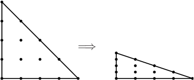
Figure 4: Squeezing the reference triangle $\widehat{K}$ perpendicularly does not deteriorate the approximation property of Lagrange interpolation.

Applying Theorem 21 to $v-\mathcal{I}_{K_{\alpha\beta}}^{k}v\in\mathcal{T}_{p}^{k}(K_{\alpha\beta})$ for $v\in W^{k+1,p}(K_{\alpha\beta})$, and obtain the following corollary.

Corollary 22

For arbitrary $v\in W^{k+1,p}(K_{\alpha\beta})$ $(1\leq p\leq\infty)$, the following estimations hold: $\displaystyle|v-\mathcal{I}_{K_{\alpha\beta}}^{k}v|_{m,p,K_{\alpha\beta}}$ $\displaystyle\leq C_{k,m,p}\left(\max\{\alpha,\beta\}\right)^{k+1-m}|v|_{k+1,p,K_{\alpha\beta}}.$

The manner of the proof of Theorem 21 is exactly similar as in the previous section. The ratio $|v|_{m,p,K_{\alpha\beta}}^{p}/|v|_{k+1,p,K_{\alpha\beta}}^{p}$ is written using the seminorms of $u$ on $\widehat{K}$, and is bounded by a constant that does not depend on $v$.

First, let $1\leq p<\infty$. For a multi-index $\gamma=(a,b)\in\mathbb{N}_{0}^{2}$ and a real $t\neq 0$, set $(\alpha,\beta)^{\gamma t}:=\alpha^{at}\beta^{bt}$. Then, we have

$$\frac{|v|_{m,p,K_{\alpha\beta}}^{p}}{|v|_{k+1,p,K_{\alpha\beta}}^{p}} =\frac{\sum_{|\gamma|=m}\frac{m!}{\gamma!}(\alpha,\beta)^{-\gamma p}\left|\partial^{\gamma}u\right|_{0,p,\widehat{K}}^{p}}{\sum_{|\delta|=k+1}\frac{(k+1)!}{\delta!}(\alpha,\beta)^{-\delta p}\left|\partial^{\delta}u\right|_{0,p,\widehat{K}}^{p}}$$

$$=\frac{\sum_{|\gamma|=m}\frac{m!}{\gamma!}(\alpha,\beta)^{-\gamma p}\left|\partial^{\gamma}u\right|_{0,p,\widehat{K}}^{p}}{\sum_{|\gamma|=m}\frac{m!}{\gamma!}(\alpha,\beta)^{-\gamma p}\left(\sum_{|\eta|=k+1-m}\frac{(k+1-m)!}{\eta!(\alpha,\beta)^{\eta p}}\left|\partial^{\eta}(\partial^{\gamma}u)\right|_{0,p,\widehat{K}}^{p}\right)}$$

$$\leq\frac{\left(\max\{\alpha,\beta\}\right)^{(k+1-m)p}\sum_{|\gamma|=m}\frac{m!}{\gamma!}(\alpha,\beta)^{-\gamma p}\left|\partial^{\gamma}u\right|_{0,p,\widehat{K}}^{p}}{\sum_{|\gamma|=m}\frac{m!}{\gamma!}(\alpha,\beta)^{-\gamma p}\left(\sum_{|\eta|=k+1-m}\frac{(k+1-m)!}{\eta!}\left|\partial^{\eta}(\partial^{\gamma}u)\right|_{0,p,\widehat{K}}^{p}\right)}$$

$$=\left(\max\{\alpha,\beta\}\right)^{(k+1-m)p}\frac{\sum_{|\gamma|=m}\frac{m!}{\gamma!}(\alpha,\beta)^{-\gamma p}\left|\partial^{\gamma}u\right|_{0,p,\widehat{K}}^{p}}{\sum_{|\gamma|=m}\frac{m!}{\gamma!}(\alpha,\beta)^{-\gamma p}\left|\partial^{\gamma}u\right|_{k+1-m,p,\widehat{K}}^{p}}.$$ (33)

Here, we used the fact that, for a multi-index $\eta$, $(\alpha,\beta)^{\eta p}\leq\left(\max\{\alpha,\beta\}\right)^{|\eta|p}$ and, for a multi-index $\delta$ with $|\delta|=k+1$,

$$\frac{|\delta|!}{\delta!}=\sum_{\begin{subarray}{c}\gamma+\eta=\delta\\ |\gamma|=m,|\eta|=k+1-m\end{subarray}}\frac{|\gamma|!}{\gamma!}\frac{|\eta|!}{\eta!}.$$

For example, if $k=2$, then we see

$$\frac{|v|_{1,p,K_{\alpha}}^{p}}{|v|_{3,p,K_{\alpha}}^{p}} =\frac{\frac{1}{\alpha^{p}}|u_{x}|_{0}^{p}+\frac{1}{\beta^{p}}|u_{y}|_{0}^{p}}{\frac{1}{\alpha^{3p}}|u_{xxx}|_{0}^{p}+\frac{3}{\alpha^{2p}\beta^{p}}|u_{xxy}|_{0}^{p}+\frac{3}{\alpha^{p}\beta^{2p}}|u_{xyy}|_{0}^{p}+\frac{1}{\beta^{3p}}|u_{yyy}|_{0}^{p}}$$

$$=\frac{\frac{1}{\alpha^{p}}|u_{x}|_{p}^{p}+\frac{1}{\beta^{p}}|u_{y}|_{p}^{p}}{\frac{1}{\alpha^{p}}\left(\frac{|u_{xxx}|_{p}^{p}}{\alpha^{2p}}+2\frac{|u_{xxy}|_{p}^{p}}{\alpha^{p}\beta^{p}}+\frac{|u_{xyy}|_{p}^{p}}{\beta^{2p}}\right)+\frac{1}{\beta^{p}}\left(\frac{|u_{xxy}|_{p}^{p}}{\alpha^{2p}}+2\frac{|u_{xyy}|_{p}^{p}}{\alpha^{p}\beta^{p}}+\frac{|u_{yyy}|_{p}^{p}}{\beta^{2p}}\right)}$$

$$\leq\frac{\max\{\alpha^{2p},\beta^{2p}\}\left(\frac{1}{\alpha^{p}}|u_{x}|_{0}^{p}+\frac{1}{\beta^{p}}|u_{y}|_{0}^{p}\right)}{\frac{1}{\alpha^{p}}\left(|u_{xxx}|_{0}^{p}+2|u_{xxy}|_{0}^{p}+|u_{xyy}|_{0}^{p}\right)+\frac{1}{\beta^{p}}\left(|u_{xxy}|_{0}^{p}+2|u_{xyy}|_{0}^{p}+u_{yyy}|_{0}^{p}\right)}$$

$$=\max\{\alpha^{2p},\beta^{2p}\}\frac{\frac{1}{\alpha^{p}}|u_{x}|_{0,p,\widehat{K}}^{p}+\frac{1}{\beta^{p}}|u_{y}|_{0,p,\widehat{K}}^{p}}{\frac{1}{\alpha^{p}}|u_{x}|_{2,p,\widehat{K}}^{p}+\frac{1}{\beta^{p}}|u_{y}|_{2,p,\widehat{K}}^{p}},$$

and

$$\frac{|v|_{2,p,K_{\alpha\beta}}^{p}}{|v|_{3,p,K_{\alpha\beta}}^{p}} =\frac{\frac{1}{\alpha^{2p}}|u_{xx}|_{0}^{p}+\frac{2}{\alpha^{p}\beta^{p}}|u_{xy}|_{0}^{p}+\frac{1}{\beta^{2p}}|u_{yy}|_{0}^{p}}{\frac{1}{\alpha^{3p}}|u_{xxx}|_{0}^{p}+\frac{3}{\alpha^{2p}\beta^{p}}|u_{xxy}|_{0}^{p}+\frac{3}{\alpha^{p}\beta^{2p}}|u_{xyy}|_{0}^{p}+\frac{1}{\beta^{3p}}|u_{yyy}|_{0}^{p}}$$

$$=\frac{\frac{1}{\alpha^{2p}}|u_{xx}|_{p}^{p}+\frac{2}{\alpha^{p}\beta^{p}}|u_{xy}|_{p}^{p}+\frac{1}{\beta^{2p}}|u_{yy}|_{p}^{p}}{\frac{1}{\alpha^{2p}}\left(\frac{|u_{xxx}|_{p}^{p}}{\alpha^{p}}+\frac{|u_{xxy}|_{p}^{p}}{\beta^{p}}\right)+\frac{2}{\alpha^{p}\beta^{p}}\left(\frac{|u_{xxy}|_{p}^{p}}{\alpha^{p}}+\frac{|u_{xyy}|_{p}^{p}}{\beta^{p}}\right)+\frac{1}{\beta^{2p}}\left(\frac{|u_{xyy}|_{p}^{p}}{\alpha^{p}}+\frac{|u_{yyy}|_{p}^{p}}{\beta^{p}}\right)}$$

$$\leq\frac{\max\{\alpha^{p},\beta^{p}\}\left(\frac{1}{\alpha^{2p}}|u_{xx}|_{0}^{p}+\frac{2}{\alpha^{p}\beta^{p}}|u_{xy}|_{0}^{p}+\frac{1}{\beta^{2p}}|u_{yy}|_{0}^{p}\right)}{\frac{1}{\alpha^{2p}}\left(|u_{xxx}|_{0}^{p}+|u_{xxy}|_{0}^{p}\right)+\frac{2}{\alpha^{p}\beta^{p}}\left(|u_{xxy}|_{0}^{p}+|u_{xyy}|_{0}^{p}\right)+\frac{1}{\beta^{2p}}\left(|u_{xyy}|_{0}^{p}+|u_{yyy}|_{0}^{p}\right)}$$

$$=\max\{\alpha^{p},\beta^{p}\}\frac{\frac{1}{\alpha^{2p}}|u_{xx}|_{0,p,\widehat{K}}^{p}+\frac{2}{\alpha^{p}\beta^{p}}|u_{xy}|_{0,p,\widehat{K}}^{p}+\frac{1}{\beta^{2p}}|u_{yy}|_{0,p,\widehat{K}}^{p}}{\frac{1}{\alpha^{2p}}|u_{xx}|_{1,p,\widehat{K}}^{p}+\frac{2}{\alpha^{p}\beta^{p}}|u_{xy}|_{1,p,\widehat{K}}^{p}+\frac{1}{\beta^{2p}}|u_{yy}|_{1,p,\widehat{K}}^{p}}.$$

In the above, we use the notation $|\cdot|_{0}$ instead of $|\cdot|_{0,p,\widehat{K}}$ for simplicity.

Exercise: Confirm the details of the above inequalities, in particular, (33).

Now suppose that, for $\mathcal{T}_{p}^{k}(\widehat{K})$ and a multi-index $\gamma$, the set $\Xi_{p}^{\gamma,k}$ is defined so that

$$u\in\mathcal{T}_{p}^{k}(\widehat{K})\Longrightarrow\partial^{\gamma}u\in\Xi_{p}^{\gamma,k}$$ (34)

and

$$A_{p}^{\gamma,k}:=\sup_{v\in\Xi_{p}^{\gamma,k}}\frac{|v|_{0,p,\widehat{K}}}{|v|_{k+1-|\gamma|,p,\widehat{K}}}<\infty$$ (35)

hold. Then, from (33), we would conclude that

$$\frac{|v|_{m,p,K_{\alpha\beta}}^{p}}{|v|_{k+1,p,K_{\alpha\beta}}^{p}} \leq\left(\max\{\alpha,\beta\}\right)^{(k+1-m)p}\frac{\sum_{|\gamma|=m}\frac{m!}{\gamma!}(\alpha,\beta)^{-\gamma p}\left|\partial^{\gamma}u\right|_{0,p,\widehat{K}}^{p}}{\sum_{|\gamma|=m}\frac{m!}{\gamma!}(\alpha,\beta)^{-\gamma p}\left|\partial^{\gamma}u\right|_{k+1-m,p,\widehat{K}}^{p}}$$

$$\leq\left(\max\{\alpha,\beta\}\right)^{(k+1-m)p}\frac{\sum_{|\gamma|=m}\left(A_{p}^{\gamma,k}\right)^{p}\frac{m!}{\gamma!}(\alpha,\beta)^{-\gamma p}\left|\partial^{\gamma}u\right|_{k+1-m,p,\widehat{K}}^{p}}{\sum_{|\gamma|=m}\frac{m!}{\gamma!}(\alpha,\beta)^{-\gamma p}\left|\partial^{\gamma}u\right|_{k+1-m,p,\widehat{K}}^{p}}$$

$$\leq\left(\max\{\alpha,\beta\}\right)^{(k+1-m)p}C_{k,m,p}^{p},\qquad C_{k,m,p}:=\max_{|\gamma|=m}A_{p}^{\gamma,k}.$$ (36)

Our task now is to define $\Xi_{p}^{\gamma,k}$ that satisfies (34) and (35). We will explain the details in the following sections.

5 Difference quotients

In this section, we define the difference quotients for two-variable functions. Our treatment is based on the theory of difference quotients of one-variable functions given in standard textbooks such as [3] and [25]. All statements in this section can be readily proved.

5.1 Difference quotients of one-variable functions

For a function $f(x)$ and nodal points $x_{0},x_{1},\cdots,x_{n}\in\mathbb{R}$, the difference quotients of $f$ are defined recursively by

$$f[x_{0},x_{1}]:=\frac{f(x_{0})-f(x_{1})}{x_{0}-x_{1}},\qquad f[x_{0},x_{1},x_{2}]:=\frac{f[x_{0},x_{1}]-f[x_{1},x_{2}]}{x_{0}-x_{2}},$$

$$f[x_{0},x_{1},\cdots,x_{m}]:=\frac{f[x_{0},\cdots,x_{m-1}]-f[x_{1},\cdots,x_{m}]}{x_{0}-x_{m}}.$$

A simplest case is $x_{i}:=x_{0}+hi$, $i=1,\cdots,m$, with $h>0$. In this case, the difference quotients are

$$f[x_{0},x_{1}]:=\frac{f(x_{1})-f(x_{0})}{h},\qquad f[x_{0},x_{1},x_{2}]:=\frac{f(x_{0})-2f(x_{1})+f(x_{2})}{h^{2}},$$

and so on. The difference quotients are expressed by integration:

$$f[x_{0},x_{1}] =\frac{1}{x_{1}-x_{0}}\int_{x_{0}}^{x_{1}}f^{\prime}(t)\text{d}t=\int_{0}^{1}f^{\prime}(x_{0}+t_{1}(x_{1}-x_{0}))\text{d}t_{1},$$

$$f[x_{0},x_{1},x_{2}] =\frac{f[x_{2},x_{1}]-f[x_{1},x_{0}]}{x_{2}-x_{0}}=\frac{f[x_{2},x_{0}]-f[x_{0},x_{1}]}{x_{2}-x_{1}}$$

$$=\frac{1}{x_{2}-x_{1}}\int_{0}^{1}\left(f^{\prime}(x_{0}+t_{1}(x_{2}-x_{0}))-f^{\prime}(x_{0}+t_{1}(x_{1}-x_{0}))\right)\text{d}t_{1}$$

$$=\int_{0}^{1}\int_{0}^{t_{1}}f^{\prime\prime}\left(x_{0}+t_{1}(x_{1}-x_{0})+t_{2}(x_{2}-x_{1})\right)\text{d}t_{2}\text{d}t_{1}.$$

For $n\geq 1$, the following formula holds:

$$f[x_{0},x_{1},\cdots,x_{n}] =\int_{0}^{1}\int_{0}^{t_{1}}\cdots\int_{0}^{t_{n-1}}f^{(n)}\left(x_{0}+\sum_{i=1}^{n}t_{i}(x_{i}-x_{i-1})\right)\text{d}t_{n}\cdots\text{d}t_{2}\text{d}t_{1}.$$ (37)

Exercise: Prove (37) by induction.

5.2 Difference quotients of two variable functions

We now extend the difference quotient to functions with two variables. For a positive integer $k$, the set $\widehat{\Sigma}^{k}\subset\widehat{K}$ is defined by

$$\widehat{\Sigma}^{k} :=\Sigma^{k}(\widehat{K}):=\left\{\mathbf{x}_{\gamma}:=\frac{\gamma}{k}\in\widehat{K}\biggm{|}\gamma\in\mathbb{N}_{0}^{2},\;0\leq|\gamma|\leq k\right\},$$

where $\gamma/k=(a_{1}/k,a_{2}/k)$ is understood as the coordinate of a point in $\widehat{\Sigma}^{k}$.

For $\mathbf{x}_{\gamma}\in\widehat{\Sigma}^{k}$ and a multi-index $\delta\in\mathbb{N}_{0}^{2}$ with $|\gamma|\leq k-|\delta|$, we define the correspondence $\Delta^{\delta}$ between nodes by

$$\Delta^{\delta}\mathbf{x}_{\gamma}:=\mathbf{x}_{\gamma+\delta}\in\widehat{\Sigma}^{k}.$$

For example, $\Delta^{(1,1)}\mathbf{x}_{(0,0)}=\mathbf{x}_{(1,1)}$ and $\Delta^{(2,1)}\mathbf{x}_{(0,1)}=\mathbf{x}_{(2,2)}$. Using $\Delta^{\delta}$, we define the difference quotients on $\widehat{\Sigma}^{k}$ for $f\in C^{0}(\widehat{K})$ by

$$f^{|\delta|}[\mathbf{x}_{\gamma},\Delta^{\delta}\mathbf{x}_{\gamma}]:=k^{|\delta|}\sum_{\eta\leq\delta}\frac{(-1)^{|\delta|-|\eta|}}{\eta!(\delta-\eta)!}f(\Delta^{\eta}\mathbf{x}_{\gamma}).$$

For simplicity, we denote $f^{|\delta|}[\mathbf{x}_{(0,0)},\Delta^{\delta}\mathbf{x}_{(0,0)}]$ by $f^{|\delta|}[\Delta^{\delta}\mathbf{x}_{(0,0)}]$. The following are examples of $f^{|\delta|}[\Delta^{\delta}\mathbf{x}_{(0,0)}]$:

$$f^{2}[\Delta^{(2,0)}\mathbf{x}_{(0,0)}] =\frac{k^{2}}{2}(f(\mathbf{x}_{(2,0)})-2f(\mathbf{x}_{(1,0)})+f(\mathbf{x}_{(0,0)})),$$

$$f^{2}[\Delta^{(1,1)}\mathbf{x}_{(0,0)}] =k^{2}(f(\mathbf{x}_{(1,1)})-f(\mathbf{x}_{(1,0)})-f(\mathbf{x}_{(0,1)})+f(\mathbf{x}_{(0,0)})),$$

$$f^{3}[\Delta^{(2,1)}\mathbf{x}_{(0,0)}] =\frac{k^{3}}{2}(f(\mathbf{x}_{(2,1)})-2f(\mathbf{x}_{(1,1)})+f(\mathbf{x}_{(0,1)})-f(\mathbf{x}_{(2,0)})$$

$$\hskip 68.8556pt+2f(\mathbf{x}_{(1,0)})-f(\mathbf{x}_{(0,0)})).$$

Let $\eta\in\mathbb{N}_{0}^{2}$ be such that $|\eta|=1$ and $\eta\leq\delta$. The difference quotients clearly satisfy the following recursive relations:

$$f^{|\delta|}[\mathbf{x}_{\gamma},\Delta^{\delta}\mathbf{x}_{\gamma}] =\frac{k}{\delta\cdot\eta}\left(f^{|\delta|-1}[\mathbf{x}_{\gamma+\eta},\Delta^{\delta-\eta}\mathbf{x}_{\gamma+\eta}]-f^{|\delta|-1}[\mathbf{x}_{\gamma},\Delta^{\delta-\eta}\mathbf{x}_{\gamma}]\right).$$

If $f\in C^{k}(\widehat{K})$, the difference quotient $f^{|\delta|}[\mathbf{x}_{\gamma},\Delta^{\delta}\mathbf{x}_{\gamma}]$ is written as an integral of $f$. Setting $d=2$ and $\delta=(0,s)$, for example, we have

$$f^{1}[\mathbf{x}_{(l,q)},\Delta^{(0,1)}\mathbf{x}_{(l,q)}]=k(f(\mathbf{x}_{(l,q+1)})-f(\mathbf{x}_{(l,q)}))=\int_{0}^{1}\partial^{(0,1)}f\left(\frac{l}{k},\frac{q}{k}+\frac{w_{1}}{k}\right)\text{d}w_{1},$$

$$f^{1}[\mathbf{x}_{(l,q)},\Delta^{(0,2)}\mathbf{x}_{(l,q)}]=\frac{k^{2}}{2}(f(\mathbf{x}_{(l,q+2)})-2f(\mathbf{x}_{(l,q+1)})+f(\mathbf{x}_{(l,q)}))$$

$$\hskip 54.06006pt=\int_{0}^{1}\int_{0}^{w_{1}}\partial^{(0,2)}f\left(\frac{l}{k},\frac{q}{k}+\frac{1}{k}(w_{1}+w_{2})\right)\text{d}w_{2}\text{d}w_{1}$$

$$\hskip 119.50148pt=k\int_{0}^{1}\left[\partial^{(0,1)}f\left(\frac{l}{k},\frac{q}{k}+\frac{2}{k}w_{1}\right)-\partial^{(0,1)}f\left(\frac{l}{k},\frac{q}{k}+\frac{1}{k}w_{1}\right)\right]\text{d}w_{1},$$

$$f^{s}[\mathbf{x}_{(l,p)},\Delta^{(0,s)}\mathbf{x}_{(l,q)}]$$

$$\hskip 28.45274pt=\int_{0}^{1}\int_{0}^{w_{1}}\cdots\int_{0}^{w_{s-1}}\partial^{(0,s)}f\left(\frac{l}{k},\frac{q}{k}+\frac{1}{k}(w_{1}+\cdots+w_{s})\right)\text{d}w_{s}\cdots\text{d}w_{2}\text{d}w_{1}.$$

To provide a concise expression for the above integral, we introduce the $s$-simplex

$$\mathbb{S}_{s}:=\left\{(t_{1},t_{2},\cdots,t_{s})\in\mathbb{R}^{s}\mid t_{i}\geq 0,\ 0\leq t_{1}+\cdots+t_{s}\leq 1\right\},$$

and the integral of $g\in L^{1}(\mathbb{S}_{s})$ on $\mathbb{S}_{s}$ is defined by

$$\int_{\mathbb{S}_{s}}g(w_{1},\cdots,w_{k})\text{d}\mathbf{W_{s}}:=\int_{0}^{1}\int_{0}^{w_{1}}\cdots\int_{0}^{w_{s-1}}g(w_{1},\cdots,w_{s})\text{d}w_{s}\cdots\text{d}w_{2}\text{d}w_{1},$$

where $\text{d}\mathbf{W_{s}}=\text{d}w_{s}\cdots\text{d}w_{2}\text{d}w_{1}$. Then, $f^{s}[\mathbf{x}_{(l,q)},\Delta^{(0,s)}\mathbf{x}_{(l,q)}]$ becomes

$$f^{s}[\mathbf{x}_{(l,q)},\Delta^{(0,s)}\mathbf{x}_{(l,q)}] =\int_{\mathbb{S}_{s}}\partial^{(0,s)}f\left(\frac{l}{k},\mathbf{W_{s}}\right)\text{d}\mathbf{W_{s}},\quad\mathbf{W_{s}}:=\frac{q}{k}+\frac{1}{k}(w_{1}+\cdots+w_{s}).$$

For a general multi-index $(t,s)$, we have

$$f^{t+s}[\mathbf{x}_{(l,q)},\Delta^{(t,s)}\mathbf{x}_{(l,q)}]=\int_{\mathbb{S}_{s}}\int_{\mathbb{S}_{t}}\partial^{(t,s)}f\left(\mathbf{Z_{t}},\mathbf{W_{s}}\right)\text{d}\mathbf{Z_{t}}\text{d}\mathbf{W_{s}}.$$

$$\mathbf{Z_{t}}:=\frac{l}{k}+\frac{1}{k}(z_{1}+\cdots+z_{t}),\quad\text{d}\mathbf{Z_{t}}:=\text{d}z_{t}\cdots\text{d}z_{2}\text{d}z_{1}.$$

Let $\square_{\gamma}^{\delta}$ be the rectangle defined by $\mathbf{x}_{\gamma}$ and $\Delta^{\delta}\mathbf{x}_{\gamma}$ as the diagonal points. If $\delta=(t,0)$ or $(0,s)$, $\square_{\gamma}^{\delta}$ degenerates to a segment. For $v\in W^{1,1}(\widehat{K})$ and $\square_{\gamma}^{\delta}$ with $\gamma=(l,q)$, we denote the integral as

$$\int_{\square_{\gamma}^{(t,s)}}v:=\int_{\mathbb{S}_{s}}\int_{\mathbb{S}_{t}}v\left(\mathbf{Z_{t}},\mathbf{W_{s}}\right)\text{d}\mathbf{Z_{t}}\text{d}\mathbf{W_{s}}.$$

If $\square_{\gamma}^{\delta}$ degenerates to a segment, the integral is understood as an integral on the segment. By this notation, the difference quotient $f^{t+s}[\mathbf{x}_{\gamma},\Delta^{(t,s)}\mathbf{x}_{\gamma}]$ is written as

$$f^{(t+s)}[\mathbf{x}_{\gamma},\Delta^{(t,s)}\mathbf{x}_{\gamma}]=\int_{\square_{\gamma}^{(t,s)}}\partial^{(t,s)}f.$$

Therefore, if $u\in\mathcal{T}_{p}^{k}(\widehat{K})$, then we have

$$0=u^{t+s}[\mathbf{x}_{\gamma},\Delta^{(t,s)}\mathbf{x}_{\gamma}]=\int_{\square_{\gamma}^{(t,s)}}\partial^{(t,s)}u,\qquad\forall\square_{\gamma}^{(t,s)}\subset\widehat{K}.$$ (38)

Exercise: Confirm that all the equations in this section certainly hold.

6 The proof of Theorem 21

By introducing the notation in the previous section, we now be able to define $\Xi_{p}^{\gamma,k}\subset W^{k+1-|\gamma|,p}(\widehat{K})$ and $A_{p}^{\gamma,k}$ for $p\in[1,\infty]$, which satisfy (34) and (35). For multi-index $\gamma$, define

$$\Xi_{p}^{\gamma,k} :=\left\{v\in W^{k+1-|\gamma|,p}(\widehat{K})\Bigm{|}\int_{\square_{lp}^{\gamma}}v=0,\quad\forall\square_{lp}^{\gamma}\subset\widehat{K}\right\}.$$

From the definition and (38), it is clear that (34) holds. Define

$$A_{p}^{\gamma,k}:=\sup_{v\in\Xi_{p}^{\gamma,k}}\frac{|v|_{0,p,\widehat{K}}}{|v|_{k+1-|\gamma|,p,\widehat{K}}},\qquad 1\leq p\leq\infty.$$

Then, the following lemma holds.

Lemma 23

We have $\Xi_{p}^{\gamma,k}\cap\mathcal{P}_{k-|\gamma|}=\{0\}$. That is, if $q\in\mathcal{P}_{k-|\gamma|}$ belongs to $\Xi_{p}^{\gamma,k}$, then $q=0$.

Proof: We notice that $\mathrm{dim}\mathcal{P}_{k-|\delta|}=\#\{\square_{lp}^{\delta}\subset\widehat{K}\}$. For example, if $k=4$ and $|\delta|=2$, then $\mathrm{dim}\mathcal{P}_{2}=6$. This corresponds to the fact that, in $\widehat{K}$, there are six squares with size $1/4$ for $\delta=(1,1)$ and there are six horizontal segments of length $1/2$ for $\delta=(2,0)$. All their vertices (corners and end-points) belong to $\Sigma^{4}(\widehat{K})$ (see Figure 5). Now, suppose that $v\in\mathcal{P}_{k-|\delta|}$ satisfies $\int_{\square_{lp}^{\delta}}q=0$ for all $\square_{lp}^{\delta}\subset\widehat{K}$. This condition is linearly independent and determines $q=0$ uniquely. $\square$

Figure 5: The six squares of size $1/4$ for $\delta=(1,1)$ and the (union of) six segments of length $1/2$ for $\delta=(2,0)$ in $\widehat{K}$.

To understand the above proof clearly, we consider the cases $k=2$ and $3$. Let $k=2$ and $\gamma=(1,0)$. Then, $k-|\gamma|=1$. Set $q(x,y)=a+bx+cy$. If the three integrals

$$\int_{\square_{00}^{(1,0)}}q(x,y)=a+\frac{b}{4},\qquad\int_{\square_{10}^{(1,0)}}q(x,y)=a+\frac{3b}{4},\qquad\int_{\square_{01}^{(1,0)}}q(x,y)=a+\frac{b}{4}+\frac{c}{2}$$

are equal to $0$, then we have $a=b=c=0$, that is, $q(x,y)=0$. The case $\gamma=(0,1)$ is similar.

Let $k=3$ and $\gamma=(1,0)$. Then, $k-|\gamma|=2$. Set $q(x,y)=a+bx+cy+dx^{2}+ey^{2}+fxy$. If the integrals

$$\int_{\square_{00}^{(1,0)}}q(x,y) =a+\frac{b}{6}+\frac{d}{27},\qquad\int_{\square_{10}^{(1,0)}}q(x,y)=a+\frac{b}{2}+\frac{7}{27}d,$$

$$\qquad\int_{\square_{20}^{(1,0)}}q(x,y) =a+\frac{5}{6}b+\frac{19}{27}d$$

are all equal to $0$, we have $a=b=d=0$. Moreover, if the integrals

$$\int_{\square_{01}^{(1,0)}}q(x,y) =\frac{c}{3}+\frac{e}{9}+\frac{f}{18},\qquad\int_{\square_{11}^{(1,0)}}q(x,y)=\frac{c}{3}+\frac{e}{9}+\frac{f}{6},$$

$$\qquad\int_{\square_{02}^{(1,0)}}q(x,y) =\frac{2}{3}c+\frac{4}{9}e+\frac{f}{9}$$

are equal to $0$ as well, we have $c=e=f=0$. Hence, we conclude that $q(x,y)=0$. The case $\gamma=(0,1)$ is similar.

Lemma 24

We have $A_{p}^{\gamma,k}<\infty$, $p\in[1,\infty]$. That is, (35) holds.

Proof: The proof is by contradiction. Suppose that $A_{p}^{\gamma,k}=\infty$. Then, there exists a sequence $\{u_{n}\}_{n=1}^{\infty}\subset\Xi_{p}^{\gamma,k}$ such that

$$|u_{n}|_{0,p,\widehat{K}}=1,\qquad\lim_{n\to\infty}|u_{n}|_{k+1-|\gamma|,p,\widehat{K}}=0.$$

By the inequality (22), for an arbitrary $\varepsilon>0$, there exists a sequence $\{q_{n}\}\subset\mathcal{P}_{k-|\gamma|}$ such that

$$\inf_{q\in\mathcal{P}_{k-|\gamma|}}\|u_{n}+q\|_{k+1-|\gamma|,p,\widehat{K}} \leq\|u_{n}+q_{n}\|_{k+1-|\gamma|,p,\widehat{K}}$$

$$\leq\inf_{q\in\mathcal{P}_{k-|\gamma|}}\|u_{n}+q\|_{k+1-|\gamma|,p,\widehat{K}}+\frac{\varepsilon}{n}$$

$$\leq C|u_{n}|_{k+1-|\gamma|,p,\widehat{K}}+\frac{\varepsilon}{n},\quad\lim_{n\to\infty}\|u_{n}+q_{n}\|_{k+1-|\gamma|,p,\widehat{K}}=0.$$

Since $|u_{n}|_{k+1-|\gamma|,p,\widehat{K}}$ and $|u_{n}|_{0,p,\widehat{K}}$ are bounded, $|u_{n}|_{m,p,\widehat{K}}$ ($1\leq m\leq k-|\gamma|$) is bounded as well by Gagliardo–Nirenberg’s inequality (Theorem 13). That is, $\|u_{n}\|_{k+1-|\gamma|,p,\widehat{K}}$ and $\{q_{n}\}\subset\mathcal{P}_{k-|\gamma|}$ are bounded. Thus, there exists a subsequence $\{q_{n_{i}}\}$ such that $q_{n_{i}}$ converges to $\bar{q}\in\mathcal{P}_{k-|\gamma|}$. In particular, we see

$$\lim_{n_{i}\to\infty}\|u_{n_{i}}+\bar{q}\|_{k+1-|\gamma|,p,\widehat{K}}=0.$$

Therefore, for any $\square_{lp}^{\gamma}$, we notice that

$$0=\lim_{n_{i}\to\infty}\int_{\square_{lp}^{\gamma}}(u_{n_{i}}+\bar{q})=\int_{\square_{lp}^{\gamma}}\bar{q},$$

and $\bar{q}=0$ by Lemma 23. This yields

$$\lim_{n_{i}\to\infty}\|u_{n_{i}}\|_{k+1-|\gamma|,p,\widehat{K}}=0,$$

which contradicts $\lim_{n_{i}\to\infty}\|u_{n_{i}}\|_{k+1-|\gamma|,p,\widehat{K}}\geq\lim_{n_{i}\to\infty}|u_{n_{i}}|_{0,p,\widehat{K}}=1$. $\square$

Now, we have defined the set $\Xi_{p}^{\gamma,k}$ that satisfies (34) and the estimate (35) has been shown. Therefore, Theorem 21 has been proved by (36).

Exercise: We have shown the Theorem 21 for the case $1\leq p<\infty$. Prove Theorem 21 for the case $p=\infty$.

7 The error estimation on general triangles in terms of circumradius

Using the previous results, we can obtain the error estimations on general triangles. Recall the reference triangle and the definition of the standard position of an aribtrary triangle $K$ (Figure 2). Let $K_{\alpha\beta}$ be the triangle with the vertices $(0,0)^{\top}$, $(\alpha,0)^{\top}$, and $(0,\beta)^{\top}$. Let $\widehat{K}$ be the reference triangle with the vertices $(0,0)^{\top}$, $(1,0)^{\top}$, and $(0,1)^{\top}$.

Figure 6: The standard position of a general triangle (reprint). The vertices are $\mathbf{x}_{1}=(0,0)^{\top}$, $\mathbf{x}_{2}=(\alpha,0)^{\top}$, and $\mathbf{x}_{3}=(\beta s,\beta t)^{\top}$, where $s^{2}+t^{2}=1$, $t>0$. We assume that $0<\beta\leq\alpha\leq h_{K}$. Then, $\pi/3\leq\theta<\pi$.

We consider $2\times 2$ matrices

$$A :=\begin{pmatrix}\alpha&\beta s\\ 0&\beta t\end{pmatrix}=\begin{pmatrix}1&s\\ 0&t\end{pmatrix}\begin{pmatrix}\alpha&0\\ 0&\beta\end{pmatrix},\quad\widetilde{A}:=\begin{pmatrix}1&s\\ 0&t\end{pmatrix},\quad D_{\alpha\beta}:=\begin{pmatrix}\alpha&0\\ 0&\beta\end{pmatrix},$$

$$A^{-1}=\begin{pmatrix}\alpha^{-1}&-\alpha^{-1}st^{-1}\\ 0&\beta^{-1}t^{-1}\end{pmatrix}=\begin{pmatrix}\alpha^{-1}&0\\ 0&\beta^{-1}\end{pmatrix}\begin{pmatrix}1&-st^{-1}\\ 0&t^{-1}\end{pmatrix},$$

and the linear transformation $\mathbf{y}=A\mathbf{x}$. The reference triangle $\widehat{K}$ is transformed to $K_{\alpha\beta}$ by $\mathbf{y}=D_{\alpha\beta}\mathbf{x}$, and $K_{\alpha\beta}$ is transformed to $K$ by $\mathbf{y}=\widetilde{A}\mathbf{x}$. Accordingly, $\mathcal{T}_{p}^{k}(K)$ is pulled-back to $\mathcal{T}_{p}^{k}(K_{\alpha\beta})$ by the mapping $\mathcal{T}_{p}^{k}(K)\ni v\mapsto\hat{v}:=v\circ\widetilde{A}$, and $\mathcal{T}_{p}^{k}(K_{\alpha\beta})$ is pulled-back to $\mathcal{T}_{p}^{k}(\widehat{K})$ by the mapping $\mathcal{T}_{p}^{k}(K)\ni v\mapsto\hat{v}:=v\circ D_{\alpha\beta}$.

By Theorem 21, for arbitrary $\alpha\geq\beta>0$ and arbitrary $p$, $1\leq p\leq\infty$, there exists a constant $C_{k,m,p}$ depending only on $k$, $m$, $p$ such that

$$B_{p}^{m,k}(K_{\alpha\beta}):=\sup_{v\in\mathcal{T}_{p}^{k}(K_{\alpha\beta})}\frac{|v|_{m,p,K_{\alpha\beta}}}{|v|_{k+1,p,K_{\alpha\beta}}}\leq\alpha^{k+1-m}C_{k,m,p}.$$ (39)

A simple computation confirms that $\widetilde{A}^{\top}\widetilde{A}$ has the eigenvalues $1\pm|s|$, and $\widetilde{A}^{-1}\widetilde{A}^{-\top}$ has the eigenvalues $(1\pm|s|)^{-1}$. That is, $\|\widetilde{A}\|=(1+|s|)^{1/2}$, $\|\widetilde{A}^{-1}\|=(1-|s|)^{-1/2}$, and $\det\widetilde{A}=t$. Therefore, defining $\hat{v}(\mathbf{x})=v(\widetilde{A}\mathbf{x})$ for $v\in\mathcal{T}_{p}^{k}(K)$, it follows from (18) that

$$|v|_{m,p,K}\leq 2^{m\mu(p)}t^{1/p}\|\widetilde{A}^{-1}\|^{m}|\hat{v}|_{m,p,K_{\alpha\beta}},$$

$$2^{-(k+1)\mu(p)}t^{1/p}\|\widetilde{A}\|^{-(k+1)}|\hat{v}|_{k+1,p,K_{\alpha\beta}}\leq|v|_{k+1,p,K}.$$

Combining the above inequalities and (39), we obtain

$$\frac{|v|_{m,p,K}}{|v|_{k+1,p,K}} \leq c_{k,m,p}\|\widetilde{A}\|^{k+1}\|\widetilde{A}^{-1}\|^{m}\frac{|\hat{v}|_{m,p,K_{\alpha\beta}}}{|\hat{v}|_{k+1,p,K_{\alpha\beta}}}$$

$$\leq c_{k,m,p}C_{k,m,p}\|\widetilde{A}\|^{k+1}\|\widetilde{A}^{-1}\|^{m}\alpha^{k+1-m},$$

where $c_{k,m,p}:=2^{(k+1+m)\mu(p)}$. Hence, we obtain the following lemma.

Lemma 25

For an arbitrary triangle $K$ in the standard position, we have $\displaystyle B_{p}^{m,k}(K)$ $\displaystyle\leq c_{k,m,p}\|\widetilde{A}\|^{k+1}\|\widetilde{A}^{-1}\|^{m}B_{p}^{m,k}(K_{\alpha\beta})$ $\displaystyle\leq c_{k,m,p}C_{k,m.p}\|\widetilde{A}\|^{k+1}\|\widetilde{A}^{-1}\|^{m}\alpha^{k+1-m},$ where $\|\widetilde{A}\|=(1+|s|)^{1/2}$ and $\|\widetilde{A}^{-1}\|=(1-|s|)^{-1/2}$.

Applying Lemma 25 to $v-\mathcal{I}_{K}^{k}v\in\mathcal{T}_{p}^{k}(K)$, we have the following corollary.

Corollary 26

For an arbitrary triangle $K$ in the standard position, we have $\displaystyle|v-\mathcal{I}_{K}^{k}v|_{m,p,K}\leq c_{k,m,p}C_{k,m.p}\|\widetilde{A}\|^{k+1}\|\widetilde{A}^{-1}\|^{m}\alpha^{k+1-m}|v|_{k+1,p,K},\quad\forall v\in W^{k+1,p}(K).$

We would like to obtain upper bounds of $\|\widetilde{A}\|$ and $\|\widetilde{A}^{-1}\|$. From Lemma 25, we obviously have $\|\widetilde{A}\|\leq\sqrt{2}$. For $\|\widetilde{A}^{-1}\|$, we observe that

$$\|\widetilde{A}^{-1}\|=\frac{1}{(1-|s|)^{1/2}} =\frac{(1+|s|)^{1/2}}{t}\qquad(\because\ s^{2}+t^{2}=1)$$

$$\leq\frac{2^{1/2}\alpha\beta h_{K}}{\alpha\beta h_{K}t}=\frac{\alpha\beta h_{K}}{2^{1/2}h_{K}|K|}\qquad\left(\because|K|=\frac{1}{2}\alpha\beta t\right)$$

$$=\frac{2^{3/2}R_{K}}{h_{K}}\qquad\left(\because R_{K}=\frac{\alpha\beta h_{K}}{4|K|}\right).$$ (40)

Thus, redefining the constant $C_{k,m,p}$, we obtain the following theorem.

Theorem 27

Suppose that a triangle $K$ is in the standard position. Let $k$, $m$ be integers with $k\geq 1$, $m=0,\cdots,k$ and $1\leq p\leq\infty$. Then, the following estimate holds: $\displaystyle B_{p}^{m,k}(K):=\sup_{v\in\mathcal{T}_{p}^{k}(K)}\frac{|v|_{m,p,K}}{|v|_{k+1,p,K}}\leq C_{k,m,p}\,\left(\frac{R_{K}}{h_{K}}\right)^{m}\alpha^{k+1-m},$ where $R_{K}$ is the circumradius of $K$, and $C_{k,m,p}$ is a constant depending only on $k$, $m$, and $p$.

Now, let $K$ be an arbitrary triangle. Note that $\alpha\leq h_{K}$ and the Sobolev norms are affected by rotations if $p\neq 2$ up to an constant (see (19)). Then, with rewriting the constant, we obtain the following corollary from Theorem 27, that is the main theorem of this survey (reprint of Theorem 13).

Corollary 28

Let $K$ be an arbitrary triangle with circumradius $R_{K}$. Let $k$ and $m$ be intergers with $k\geq 1$ and $m=0,\cdots,k$. Let $p$, $1\leq p\leq\infty$. For the Lagrange interpolation $\mathcal{I}_{K}^{k}v$ of degree $k$ on $K$, the following estimate holds: for any $v\in W^{2,p}(K)$, $\displaystyle B_{p}^{m,k}(K):=\sup_{u\in\mathcal{T}_{p}^{k}(K)}\frac{|u|_{m,p,K}}{|u|_{k+1,p,K}}\leq\,C_{k,m,p}\left(\frac{R_{K}}{h_{k}}\right)^{m}h_{K}^{k+1-m},$ $\displaystyle|v-\mathcal{I}_{K}^{k}v|_{m,p,K}\leq C_{k,m,p}\left(\frac{R_{K}}{h_{K}}\right)^{m}h_{K}^{k+1-m}|v|_{k+1,p,K},$ where $C_{k,m,p}$ depends only on $k$, $m$, and $p$.

Remarks: (1) Let $\Omega\subset\mathbb{R}^{2}$ be a bounded polygonal domain. We compute a numerical solution of the Poisson equation

$$-\Delta u=f\text{ in }\Omega,\quad u=0\text{ on }\partial\Omega$$

by the conforming piecewise $k$th-order finite element method on simplicial elements. To this end, we construct a triangulation $\mathcal{T}_{h}$ of $\Omega$ and consider the piecewise $\mathcal{P}_{k}$ continuous function space $S_{h}\subset H_{0}^{1}(\Omega)$. The weak form of the Poisson equation is

$$\int_{\Omega}\nabla u\cdot\nabla v\text{d}\mathbf{x}=\int_{\Omega}fv\text{d}\mathbf{x},\quad\forall v\in H_{0}^{1}(\Omega),$$

and the finite element solution is defined as the unique solution $u_{h}\in S_{h}$ of

$$\int_{\Omega}\nabla u_{h}\cdot\nabla v_{h}\text{d}\mathbf{x}=\int_{\Omega}fv_{h}\text{d}\mathbf{x},\quad\forall v_{h}\in S_{h}.$$

Céa’s Lemma implies that the error $|u-u_{h}|_{1,2,\Omega}$ is estimated as

$$|u-u_{h}|_{1,2,\Omega}\leq\left(\sum_{K\in\mathcal{T}_{h}}|u-\mathcal{I}_{K}^{k}u|_{1,2,K}^{2}\right)^{1/2}.$$ (41)

Combining (41) and Corollary 28 with $p=2$, $k\geq 2$, $m=1$, we have

$$|u-u_{h}|_{1,2,\Omega} \leq C\left(\sum_{K\in\mathcal{T}_{h}}|u-\mathcal{I}_{K}^{k}u|_{k+1,2,K}^{2}\right)^{1/2}$$

$$\leq C\left(\sum_{K\in\mathcal{T}_{h}}(R_{K}h_{K}^{k-1})^{2}|u|_{k+1,2,K}^{2}\right)^{1/2}$$

$$\leq C\max_{K\in\mathcal{T}_{h}}(R_{K}h_{K}^{k-1})|u|_{k+1,2,\Omega}.$$

Therefore, if $\max_{K\in\mathcal{T}_{h}}(R_{K}h_{K}^{k-1})\to 0$ as $h\to 0$ and $u\in H^{k+1}(\Omega)$, the finite element solution $u_{h}$ converges to the exact solution $u$ even if there exist many skinny elements violating the shape regularity condition or the maximum angle condition in $\mathcal{T}_{h}$.

Recall the triangle depicted in Figure 3 (right) with vertices $(0,0)^{\top}$, $(h,0)^{\top}$, and $(h^{\alpha},h^{\beta})^{\top}$ with $R_{K}=\mathcal{O}(h^{1+\alpha-\beta})$. Suppose now that $\alpha+1\leq\beta<2+\alpha$. If a sequence of triangulations contains those triangles, and $k=1$, then $\max_{K\in\mathcal{T}_{h}}R_{K}=\mathcal{O}(1)$ and the piecewise linear Lagrange FEM might not converge. However, if $k=2$, then $\max_{K\in\mathcal{T}_{h}}(R_{K}h_{K})=\mathcal{O}(h^{2+\alpha-\beta})$, and the finite element solution certainly converges to the exact solution, although the convergence rate is worse than expected. This means that “bad” triangulations with many very skinny triangles can be remedied by using higher-order Lagrange elements.

8 Numerical experiments

To confirm the results obtained, we perform numerical experiments similar to those in [11]. Let $\Omega:=(-1,1)\times(-1,1)$, $f(x,y):=a^{2}/(a^{2}-x^{2})^{3/2}$, and $g(x,y):=(a^{2}-x^{2})^{1/2}$ with $a:=1.1$. Then we consider the following Poisson equation: Find $u\in H^{1}(\Omega)$ such that

$$-\Delta u=f\quad\text{ in }\Omega,\qquad u=g\quad\text{ on }\partial\Omega.$$ (42)

The exact solution of (42) is $u(x,y)=g(x,y)$ and its graph is a part of the cylinder. For a given positive integer $N$ and $\alpha>1$, we consider the isosceles triangle with base length $h:=2/N$ and height $2/\lfloor 2/h^{\alpha}\rfloor\approx h^{\alpha}$, as shown in Figure 7. Let $R$ be the circumradius of the triangle. For comparison, we also consider the isosceles triangle with base length $h$ and height $h/2$ for $\alpha=1$. We triangulate $\Omega$ with this triangle, as shown in Figure 7. Let $\tau_{h}$ be the triangulation. As usual, the set $S_{h}$ of piecewise linear functions on $\tau_{h}$ and its subsets are defined by

$$S_{h} :=\left\{v_{h}\in C(\overline{\Omega})\bigm{|}v|_{K}\in\mathcal{P}_{1}(K),\;\forall K\in\tau_{h}\right\},$$ (43)

$$S_{hg} :=\left\{v_{h}\in S_{h}\bigm{|}v_{h}=g\;\text{at boundary nodes}\right\},$$ (44)

$$S_{h0} :=\left\{v_{h}\in S_{h}\mid v_{h}=0\text{ on }\partial\Omega\right\}.$$ (45)

Then, the piecewise linear finite element method for (42) is defined as follows: Find $u_{h}\in S_{hg}$ such that

$$(\nabla u_{h},\nabla v_{h})_{\Omega}=(f,v_{h})_{\Omega},\quad\forall v_{h}\in S_{h0},$$

where $(\cdot,\cdot)_{\Omega}$ is the inner product of $L^{2}(\Omega)$. By Céa’s lemma and the result obtained, we obtain the estimation

$$|u-u_{h}|_{1,2,\Omega}\leq\inf_{v_{h}\in S_{hg}}|u-v_{h}|_{1,2,\Omega}\leq\left(\sum_{K\in\tau_{h}}|u-\mathcal{I}_{K}^{1}u|_{1,2,K}^{2}\right)^{1/2}\leq CR|u|_{2,2,\Omega}.$$ (46)

The behavior of the error is given in Figure 7. The horizontal axis represents the mesh size measured by the maximum diameter of triangles in the meshes and the vertical axis represents the error associated with FEM solutions in the $H^{1}$ semi-norm. The graph clearly shows that the convergence rates worsen as $\alpha$ approaches $2.0$. For $\alpha=2.1$, the FEM solutions even diverge. This is a counterexample to the vaguely believed dogma that “FEM solutions always converge to the exact solution if $h\to 0$”. See also [23].

We replot the same data in Figure 8, in which the horizontal axis represents the maximum of the circumradius of triangles in the meshes. Figure 8 shows convergence rates are almost the same in all cases if we measure these with the circumradius. These experiments strongly support that our theoretical results are correct and optimal.

Figure 7: Triangulation of $\Omega$ with $N=12$ and $\alpha=1.6$, and the errors for FEM solutions in the $H^{1}$-norm. The horizontal axis represents the maximum diameter of the triangles and the vertical axis represents the $H^{1}$-norm of the errors of the FEM solutions. The number next to the symbol indicates the value of $\alpha$.

Figure 8: Replotted data: the errors in the $H^{1}$-norm of FEM solutions measured using the circumradius. The horizontal axis represents the maximum circumradius of the triangles.

Acknowledgments
We thank Dr. Théophile Chaumont-Frelet for his valuable comments.

References

[1]R.A. Adams, J.J.F. Fournier:
Sobolev Spaces, 2nd edition, Pure and Applied Mathematics 140,
Elsevier/Academic Press, New York, 2003.
[2]T. Apel:
Anisotropic Finite Element: Local estimates and applications,
Advances in Numerical Mathematics.
B.G. Teubner, Stuttgart, 1999.
[3]K.E. Atkinson:
An Introduction to Numerical Analysis, 2nd edition,
John Wiley & Sons, New York, 1989.
[4]I. Babuška, A.K. Aziz:
On the angle condition in the finite element method,
SIAM J. Numer. Anal. 13 (1976), 214–226.
[5]R.E. Barnhill, J.A. Gregory:
Sard kernel theorems on triangular domains with application to
finite element error bounds.
Numer. Math., 25 (1976), 215-229.
[6]S.C. Brenner, L.R. Scott:
The Mathematical Theory of Finite Element Methods. 3rd edition.
Texts in Applied Mathematics 15,
Springer, New York, 2008.
[7]H. Brezis:
Functional Analysis, Sobolev Spaces and Partial Differential
Equations. Universitext, Springer, New York, 2011.
[8]P.G. Ciarlet:
The Finite Element Methods for Elliptic Problems.
Classics in Applied Mathematics 40, SIAM, Philadelphia, 2002,
Reprint of the 1978 original (North Holland, Amsterdam).
[9]J. Brandts, S. Korotov, M. Křížek:
On the equivalence of regularity criteria for triangular and
tetrahedral finite element partitions, Comput. Math. Appl. 55 (2008), 2227–2233.
[10]A. Ern, J-L. Guermond:
Theory and Practice of Finite Elements.
Applied Mathematical Sciences 159, Springer, New York, 2004.
[11]A. Hannukainen, S. Korotov, M. Křížek:
The maximum angle condition is not necessary for convergence of
the finite element method,
Numer. Math., 120, 79–88 (2012)
[13]P. Jamet:
Estimations d’erreur pour des elements finis droits
presque degeneres. R.A.I.R.O. Anal. Numer., 10
(1976), 43–61.
[14]K. Kobayashi:
On the interpolation constants over triangular elements
(in Japanese), RIMS Kokyuroku, 1733 (2011), 58-77.
[15]K. Kobayashi, T. Tsuchiya:
A Babuška-Aziz type proof of the circumradius condition,
Japan J. Indust. Appl. Math., 31 (2014), 193-210.
[16]K. Kobayashi, T. Tsuchiya:
On the circumradius condition for piecewise linear triangular elements,
Japan J. Indust. Appl. Math., 32 (2015), 65–76.
[17]K. Kobayashi, T. Tsuchiya:
A priori error estimates for Lagrange interpolation
on triangles. Appl. Math., Praha 60 (2015), 485–499.
[18]K.Kobayashi, T.Tsuchiya:
Extending Babuška-Aziz’s theorem to higher order Lagrange
interpolation,
Appl. Math., Praha 61 (2016), 121–133.
[19]M. Křížek:
On semiregular families of triangulations and linear interpolation.
Appl. Math., Praha 36 (1991), 223–232.
[20]M. Křížek:
On the maximum angle condition for linear tetrahedral elements.
SIAM J. Numer. Anal., 29 (1992), 513–520.
[21]A. Kufner, O. John, S. Fučík:
Function Spaces.
Noordhoff International Publishing, Leyden, 1977.
[22]X. Liu, F. Kikuchi:
Analysis and estimation of error constants for and
interpolation over triangular finite element,
J. Math. Sci. Univ. Tokyo, 17 (2010), 27–78.
[23]P. Oswald:
Divergence of fem: Babuška-Aziz triangulations revisited,
Appl. Math., Praha 60 (2015), 473–484.
[24]N.A. Shenk:
Uniform error estimates for certain narrow Lagrange finite elements.
Math. Comp., 63 (1994), 105–119.
[25]T. Yamamoto:
Introduction to Numerical Analysis, 2nd edition,
(In Japanese),
Saiensu-sha,
2003.
[26]T. Yamamoto:
Elements of Matrix Analysis (in Japanese),
Saiensu-sha,
2010.
[27]A. Ženíšek: The convergence of the finite element method
for boundary value problems of a system of elliptic equations. (in Czech)
Appl. Math., 14 (1969), 355–377.
[28]M. Zlámal:
On the finite element method,
Numer. Math. 12 (1968), 394–409.