$T^{3}$-Stern-Gerlach Matter-Wave Interferometer

Abstract

We present a unique matter-wave interferometer whose phase scales with the cube of the time the atom spends in the interferometer. Our scheme is based on a full-loop Stern-Gerlach interferometer incorporating four magnetic field gradient pulses to create a state-dependent force. In contrast to typical atom interferometers which make use of laser light for the splitting and recombination of the wave packets, this realization uses no light and can therefore serve as a high-precision surface probe at very close distances.

Introduction.– The Stern-Gerlach (SG) effect Gerlach1922 of 1922 is a paradigm of quantum mechanics and allows an illuminating glimpse Schwinger2001 into the inner workings of this theory. Moreover, it arguably marks the birth of atom interferometry Berman1997 ; Cronin2009 . Indeed, the splitting of an atomic beam by a magnetic field gradient served as the starting point for David Bohm Bohm1951 and Eugene Paul Wigner Wigner1963 in their discussion of the coherence in a SG interferometer (SGI). A detailed analysis Englert1988 ; Schwinger1988 ; Scully1989 of such a device concluded that it would require an extreme accuracy of the field gradients to maintain coherence, a formidable challenge appropriately coined the Humpty Dumpty effect.

In the present Letter we report on the successful implementation of an SGI utilizing the strong and accurate magnetic field gradients Machluf2013 ; Margalit2018 provided by the currents in the wires of an atom chip Keil2016 . Our SGI is unique in three aspects: (i) Although the gradient fields act on the atom continuously during its flight through the interferometer, as in the Humpty-Dumpty configuration Englert1988 ; Schwinger1988 ; Scully1989 , we obtain a remarkably high contrast. (ii) The observed phase shift scales Zimmermann2017 with the cube of the time the atom spends in the SGI, and thus represents the first interferometric measurement of the Kennard phase Kennard1927 ; Kennard1929 ; Rozemann2019 predicted in 1927. (iii) The lack of light pulses to split and recombine the beams in combination with the Kennard phase makes our interferometer a perfect probe for magnetic as well as other properties of surfaces.

In general, the phase of spatial light-pulse atom interferometers Berman1997 ; Cronin2009 does not display a pure $T^{3}$-scaling, where $T$ is the total interferometer time. For example, in the Ramsey-Bordé interferometer BORDE1989 , the phase shift originates from a constant position difference between two paths, which in the presence of a time-independent linear potential leads to a phase proportional to $T$. In the Kasevich-Chu interferometer Kasevich1991 ; Peters2001 , it is caused by a piece-wise constant momentum difference leading to a $T^{2}$-scaling. However, our $T^{3}$-SGI has a piece-wise constant acceleration difference between its two paths resulting in a phase scaling as $T^{3}$.

Phase contributions scaling with $T^{3}$ emerge also in other setups and originate, for example, from rotation in a Sagnac interferometer Dutta2016 , the presence of a gravity gradient Kasevich2017 or a time-dependent acceleration induced by Bloch oscillations McDonald2014 in the Kasevich-Chu configuration. However, our $T^{3}$-SGI has a pure $T^{3}$-scaling resulting from the imprinted state-dependent linear potentials.

Probing surfaces with sensitive matter-waves is a long standing goal. Previous studies have probed short-distance phenomena such as Casimir-Polder forces Harber2005 ; Slama2010 , Johnson noise Jones2003 ; Blatt2015 , patch potentials Blatt2015 ; Chan2014 ; Lakhmanskiy2019 , and exotic physics such as the fifth force Sorrentino2009 ; Santos2018 ; comment-Santos . Matter-wave interferometry near the surface can significantly increase the sensitivity. Unlike a light-based atom interferometer, which cannot operate close to the surface due to light scattering from the nearby object, the SGI does not require any laser light in order to control a coherent spatial superposition of two atomic wave packets. As the accumulated phase is sensitive to magnetic fields, the SGI may be used as a unique probe for magnetic surface properties, as well as for noise and order parameters in electron transport such as squeezed currents. In addition, in a “matter-wave homodyne” type scheme, one wave packet may be put in the vicinity of the surface while the other acts as a reference.

Setup.– Our experiment is based on what is, to the best of our knowledge, the first full-loop SGI realization Margalit2018 , as originally envisioned Bohm1951 ; Wigner1963 . Different from previous realizations of the SG effect Gerlach-optics1 ; Gerlach-optics2 , it uses four magnetic field gradient operations for splitting, stopping, accelerating back, and stopping for a complete closure of a full-loop. The experiment begins with a ⁸⁷Rb Bose-Einstein condensate (BEC) released from a magnetic trap and falling freely under gravity. We define our coordinate system such that the $z$-axis is along the gravitational acceleration of magnitude $g$. The non-linear Zeeman effect of a bias magnetic field $B_{0}$ of $35$ G along the $y$-axis, added by an external pair of Helmholtz coils, creates an effective two-level system consisting of the states $|1\rangle\equiv|F=2,m_{F}=1\rangle$ and $|2\rangle\equiv|F=2,m_{F}=2\rangle$ of the $5^{2}S_{1/2}$ manifold. Since the BEC quickly expands after its release from the magnetic trap, the interatomic interactions are negligible and the experiment may be considered a single-particle experiment.

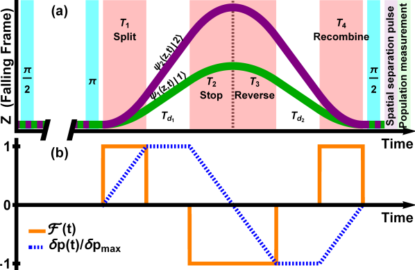
Figure 1: Pulse sequence of our longitudinal $T^{3}$-SGI (not to scale). (a) Center-of-mass trajectories of the atomic wave packets with internal states $|1\rangle$ (bottom, green) and $|2\rangle$ (top, purple). Also shown are the $\pi/2$ and $\pi$ RF (light blue) and magnetic gradient splitting, stopping, reversing and recombining pulses (light red). The magnetic field gradients result in a state-dependent force along the z-direction while the strong bias magnetic field along the y-direction defines the quantization axis. (b) Time-dependence of the relative force ${\mathcal{F}}\equiv{\mathcal{F}}(t)$, Eq. (3), (orange curve) and the corresponding relative momentum $\delta p(t)=\mathcal{P}_{2}(t)-\mathcal{P}_{1}(t)$, (blue dashed curve) between the wave packets moving along the two interferometer paths. In the experiment, we have achieved the maximal separations $\delta z_{\rm{max}}=1.4$ $\mu$m and $\delta p_{\rm{max}}/m_{Rb}=19$ mm/s in position and velocity.

After being released, the initially prepared atomic internal state $|2\rangle$ is transferred to an equal superposition, $|\phi_{\pi/2}\rangle\equiv(|1\rangle+|2\rangle)/\sqrt{2}$, by an on-resonance radio-frequency (RF) $\pi/2$-pulse, as shown in Fig. 1. Following a free-fall time of $400\,\mu$s, named hereafter the dark time, we apply an RF $\pi$-pulse that flips the atomic state to $(|1\rangle-|2\rangle)/\sqrt{2}$. After a second dark time of another $400\,\mu$s, the second RF $\pi/2$-pulse completes the echo sequence. Using a long magnetic field gradient and standard absorption imaging, we measure the relative populations of the states.

The interferometric scheme realized during the second dark time consists of four magnetic field gradient pulses produced by three parallel gold wires along the $x$-axis on the atom chip Margalit2018 . The currents running through them in alternating directions are identical and create a two-dimensional quadrupole field in the $yz$ plane with its center (zero) at $z_{0}=98\,\mu$m below the chip surface.

The first gradient pulse, applied for a duration of $T_{1}$, prepares the state of the atomic center-of-mass motion in the form of two wave packets taking separate trajectories. Indeed, close to the center, the wave packets experience different forces ${\bf F}_{i}=\mu_{i}(\partial B_{y}/\partial z){\bf e}_{z}$ where $\mu_{i}\equiv\langle i|{\hat{\mu}_{y}}|i\rangle=\mu_{B}g_{F_{i}}m_{F_{i}}$ is the mean value of the magnetic dipole moment of the state $|i\rangle$ with $i=1,2$. Here $\mu_{B}$, $g_{F}$, and $m_{F}$ denote the Bohr magneton, the Landé factor, and the projection of the angular momentum on the $y$-axis, respectively.

After a delay time, $T_{d_{1}}=T_{d}$, which is limited by the speed of our electronic circuits, we apply a second and third pulse back-to-back of identical duration, $T_{2}=T_{3}=T_{1}$. This combined pulse, having opposite polarity (the direction of the magnetic field gradient) to the first pulse thereby applying a force in the opposite direction, first compensates the momentum difference between the two wave packets, and then reverses the direction of their motion. A fourth pulse applied after another delay time, $T_{d_{2}}=T_{d}$, for a duration $T_{4}=T_{1}$, with the same polarity as the first pulse, leads to an interferometer which is closed both in momentum and position.

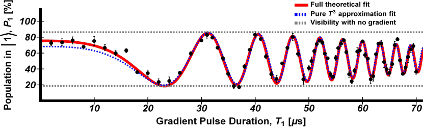
Figure 2: Measurement of the cubic phase with the $T^{3}$-SGI presented in Fig. 1. The solid red line represents a fit based on Eqs. (8) and (9) to the experimental data (dots), where the fitting parameters are the decay constant, the magnetic acceleration $a_{B}$, and a constant phase $\varphi_{0}$. The dashed blue line is a fit based on Eq. (9) with $T_{d}=0$, leading to a pure $T_{1}^{3}$ scaling of the interferometer phase as seen in Eq. (10). The visibility drops from $68\%$ to $32\%$ over $70\,\mu{\rm s}$ with a decay time of $75\,\mu{\rm s}$. This reduction results from inaccuracies in recombining the two interferometer paths. The dashed gray horizontal lines depict the maximal and minimal values of the population $P_{1}$ measured without magnetic field gradients.

Phase of interferometer.– In the $T^{3}$-SGI, no transitions occur during the four gradient pulses, as shown in Fig. 1. Hence, the complete quantum state

$$|\Psi(t)\rangle=\frac{1}{\sqrt{2}}\left[|1\rangle\hat{U}_{1}(t,0)|\psi(0)\rangle-|2\rangle\hat{U}_{2}(t,0)|\psi(0)\rangle\right]$$ (1)

is determined by the state $|\psi(0)\rangle$ of the center-of-mass motion directly after the $\pi$-pulse, with $\langle\psi(0)|\psi(0)\rangle=1$, together with the time evolution operator $\hat{U}_{i}$ for the internal state $|i\rangle$ corresponding to the time-dependent potential

$$V_{i}(z,t)\equiv-\left[mg+\mu_{i}\frac{\partial B_{y}}{\partial z}\mathcal{F}(t)\right]z$$ (2)

where $m$ is the atomic mass.

Moreover, the time dependence

$${\mathcal{F}}(t)\equiv\Theta(t)-\Theta(t-T_{1})-\Theta(t-T_{1}-T_{d})+\Theta(t-3T_{1}-T_{d})$$

$$+\Theta(t-3T_{1}-2T_{d})-\Theta(t-4T_{1}-2T_{d}),$$ (3)

displayed in Fig. 1(b) by the orange curve involves the Heaviside step function $\Theta(t)$.

Since $V_{i}$ is linear in the coordinate $z$, we can obtain the explicit expression Zimmermann2019

$$\hat{U}_{i}(t,0)\equiv e^{i\Phi_{i}(t)}\hat{D}\left[\mathcal{Z}_{i}(t),\mathcal{P}_{i}(t)\right]\hat{U}_{0}(t,0)$$ (4)

for $\hat{U}_{i}$ which consists of the product of (i) the time evolution operator $\hat{U}_{0}(t,0)\equiv\exp\left[-it\hat{p}_{z}^{2}/(2m\hbar)\right]$ of the center-of-mass motion of the free atom, (ii) the displacement operator $\hat{D}\left[\mathcal{Z},\mathcal{P}\right]\equiv\exp\left[(i/\hbar)\left(\mathcal{P}\hat{z}-\mathcal{Z}\hat{p}_{z}\right)\right]$ with

$$\mathcal{P}_{i}(t)\equiv-\int\limits_{0}^{t}d\tau\frac{\partial V_{i}}{\partial z}\;\;\;{\rm and}\;\;\;\mathcal{Z}_{i}(t)\equiv-\frac{1}{m}\int\limits_{0}^{t}d\tau(t-\tau)\frac{\partial V_{i}}{\partial z},$$ (5)

as well as the position $\hat{z}$ and momentum $\hat{p}_{z}$ operators, and (iii) a phase factor

$$\Phi_{i}(t)\equiv-\frac{1}{2\hbar}\int\limits_{0}^{t}d\tau\mathcal{Z}_{i}(\tau)\frac{\partial V_{i}}{\partial z}.$$ (6)

The second $\pi/2$-pulse applied at $t=T\equiv 4T_{1}+2T_{d}$ recombines both branches of the interferometer, and the probability $P_{1}\equiv\langle\psi_{1}(T)|\psi_{1}(T)\rangle$ to observe atoms in the internal state $|1\rangle$ follows from the state $|\psi_{1}(T)\rangle\equiv\langle\phi_{\pi/2}|\Psi(T)\rangle$ of the atomic center-of-mass motion, which according to Eq. (1) takes the form

$$|\psi_{1}(T)\rangle = \frac{1}{2}\left\{e^{i\Phi_{1}(T)}\hat{D}\left[\mathcal{Z}_{1}(T),\mathcal{P}_{1}(T)\right]\right.$$ (7)

$$- \left.e^{i\Phi_{2}(T)}\hat{D}\left[\mathcal{Z}_{2}(T),\mathcal{P}_{2}(T)\right]\right\}\hat{U}_{0}(T,0)|\psi(0)\rangle.$$

From Eqs. (5) and (3) we note that the two branches overlap in both momentum and position, that is $\mathcal{P}_{1}(T)=\mathcal{P}_{2}(T)$ and $\mathcal{Z}_{1}(T)=\mathcal{Z}_{2}(T)$, as depicted in Fig. 1, leading to identical displacement operators in Eq. (7). Hence, the probability

$$P_{1}=\frac{1}{2}\left[1-\cos\left(\delta\Phi+\varphi_{0}\right)\right]$$ (8)

contains the interferometer phase $\delta\Phi\equiv\Phi_{1}(T)-\Phi_{2}(T)$ given explicitly by

$$\delta\Phi=\frac{mga_{B}}{\hbar}\left(\frac{\mu_{1}-\mu_{2}}{\mu_{B}}\right)\left(2T_{1}^{3}+3T_{1}^{2}T_{d}+T_{1}T_{d}^{2}\right)$$

$$+\frac{ma_{B}^{2}}{\hbar}\left(\frac{\mu_{1}^{2}-\mu_{2}^{2}}{\mu_{B}^{2}}\right)\left(\frac{2}{3}T_{1}^{3}+T_{1}^{2}T_{d}\right).$$ (9)

Here $\varphi_{0}$ is a constant phase taking into account possible technical misalignment and $a_{B}\equiv(\mu_{B}/m)(\partial B_{y}/\partial z)$.

In this derivation we have made two assumptions: (i) Close to the center, the magnetic field generated by the three-wire configuration is linear, and (ii) the lengths of the four gradient pulses are identical, that is $T_{2,3,4}=T_{1}$, and so are the two delay times, $T_{d_{1}}=T_{d_{2}}=T_{d}$.

Assumption (i) holds true when the distance ($\sim 1\,\mu$m) traveled by the atomic wave packets is small compared to the distance ($\sim 100\,\mu$m) from the chip. In our current apparatus, a violation of this constraint and the resulting magnetic field non-linearity gives rise to a $3.5\%$ change in the applied force. Future improvements of the experiment will be required to address this issue.

Regarding assumption (ii), we have slightly adjusted the length of $T_{4}$, in order to better optimize the visibility and account for the non-linearity, up to a difference of $8\%$ from $T_{1}$.

Measurement of the cubic interferometer phase.– Nevertheless, the experimental data (dots) depicted in Fig. 2 agree very well with the theory (solid red line) based on Eq. (9), where the fitting parameters are the decay constant of the visibility, the magnetic field gradient $\partial B_{y}/\partial z$ or $a_{B}$, and a constant phase $\varphi_{0}$. The dashed blue line is a fit based on Eq. (9) with $T_{d}=0$, leading to a pure cubic scaling T3-comment

$$\delta\Phi^{(T^{3})}\cong\frac{ma_{B}}{32\hbar}\left(\frac{\mu_{1}-\mu_{2}}{\mu_{B}}\right)\left(g+\frac{\mu_{1}+\mu_{2}}{3\mu_{B}}\,a_{B}\right)T^{3}$$ (10)

of the interferometer phase with the total time $T\cong 4T_{1}$. In our experiment $T_{d}=2.6\,\mu$s, with $T_{1}$ having a maximal value of $70\,\mu$s.

The maximum contrast displayed by the gray lines is first measured by performing only the spin-echo sequence ($\pi/2-\pi-\pi/2$) without the magnetic field gradients and changing the phase of the closing RF $\pi/2$-pulse. The maximal visibility is limited by imperfections in the RF pulses. The echo sequence also allows us to cancel out the contribution to the interferometer phase from the bias magnetic field, and to increase the coherence time.

As a result, this interferometric technique allows us to measure the magnetic field acceleration, $a_{B}^{fit}=273.16\pm 0.09$ ${\rm m/s^{2}}$. On the other hand, the magnetic field gradient $\partial B_{y}/\partial z$ was determined independently by the time-of-flight (TOF) technique where the atomic ensemble is released from the magnetic trap, and a single magnetic field gradient pulse is applied. Measuring the final position of the atomic ensemble after some TOF, we obtain $a_{B}^{TOF}=271\pm 6$ ${\rm m/s^{2}}$. The difference in measurement errors clearly shows that our $T^{3}$-SGI provides a precise measurement of the magnetic field gradient.

Due to the stable current in the external coils, the fluctuations of the homogeneous bias field are relatively small. The phase noise is mainly proportional to the amplitude of the magnetic field of the gradient pulses originating from the chip currents Machluf2013 . Positioning the atoms near the center of the magnetic field quadrupole created solely by the three chip wires, reduces the phase noise considerably Margalit2018 . The fluctuations are further reduced due to the fact that the chip wire current is driven by batteries which supply a stable voltage modulated using a home-made current shutter. Shot-to-shot charge fluctuations are measured to be $\delta Q/Q=3.6\cdot 10^{-3}$ where $Q$ is the total charge in a single pulse.

Next we consider the case when $T_{1}\ll T_{d}$ and keep the absolute value of the relative momentum $\delta p_{0}\equiv ma_{B}T_{1}(\mu_{1}-\mu_{2})/\mu_{B}$ between the two paths constant, that is we take the magnetic field gradient pulses to be a delta function. In this limit the interferometer phase

$$\delta\Phi^{(T^{2})}\cong\frac{\delta p_{0}}{4\hbar}\,gT^{2}$$ (11)

following from Eq. (9) scales quadratically with the total time $T\cong 2T_{d}$, since we maintain a piece-wise constant momentum difference between the two arms similar to the $T^{2}$-SGI Margalit2018 , or the Kasevich-Chu interferometer Zimmermann2019 . However, in the case of the $T^{2}$-SGI the momentum transfer $\delta p_{0}$ is provided by the magnetic field gradient rather than the laser light pulse.

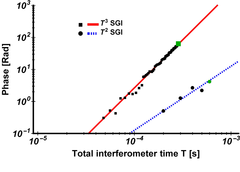
Figure 3: Comparison between the scalings of the interferometer phases $\delta\Phi^{(T^{3})}$ (solid red curve) and $\delta\Phi^{(T^{2})}$ (dashed blue curve) given by Eqs. (10) and (11), respectively. The squares are data from Fig. 2, while the dots are from our $T^{2}$-SGI realization Margalit2018 . The green square represents the largest accumulated phase of the $T^{3}$-SGI in its current configuration with $T_{\rm max}=285\,\mu{\rm s}$ at the point of $\approx 30\%$ contrast. As a reference, the green dot indicates the largest accumulated phase observed with a $T^{2}$-SGI also at $\approx 30\%$ contrast. The latter is significantly smaller although the magnetic field gradients and the maximal time $T_{\rm max}=924\,\mu{\rm s}$ are larger than those of the $T^{3}$-SGI by a factor of 2.3 and 3.2, respectively differences .

Finally, in Fig. 3 we compare the scaling of the interferometer phases $\delta\Phi^{(T^{3})}$ (solid red curve) and $\delta\Phi^{(T^{2})}$ (dashed blue curve) given by Eqs. (10) and (11), respectively. In squares are the data points from Fig. 2 and in dots are data from our $T^{2}$-SGI Margalit2018 . It is clear that the $T^{3}$-SGI significantly outperforms the $T^{2}$-SGI with respect to total phase accumulation.

Summary.– We have realized a novel matter-wave interferometer, being unique in several ways: (i) It opens a road towards testing the Humpty-Dumpty hypothesis, (ii) The phase scales purely as $T^{3}$, constituting an observation of the Kennard phase, and (iii) It does not utilize light to create beam splitters and mirrors, enabling a novel probe. A future challenge will be to find configurations with this, or even an improved, phase scaling, which are more sensitive to external forces.

- (1) W. Gerlach and O. Stern, “Der experimentelle Nachweis der Richtungsquantelung im Magnetfeld.” Z. Phys. 9, 349 (1922).
- (2) J. Schwinger, “Quantum Mechanics.” (Springer, Berlin Heidelberg, 2001).
- (3) “Atom Interferometry.” ed. by P.R. Berman (Academic Press, San Diego, 1997).
- (4) A. D. Cronin, J. Schmiedmayer, and D. E. Pritchard, “Optics and interferometry with atoms and molecules.” Rev. Mod. Phys. 81, 1051 (2009).
- (5) D. Bohm, “Quantum Theory,” (Prentice-Hall, Englewood Cliffs, 1951), p. 604-605.
- (6) E. P. Wigner, “The Problem of Measurement.” Am. J. Phys. 31, 6 (1963).
- (7) B.-G. Englert, J. Schwinger, and M.O. Scully, “Is spin coherence like Humpty-Dumpty? I. Simplified treatment.” Found. Phys. 18, 1045 (1988).
- (8) J. Schwinger, M.O. Scully, and B.-G. Englert, “Is spin coherence like Humpty-Dumpty? II. General theory.” Z. Phys. D 10, 135 (1988).
- (9) M. O. Scully, B.-G. Englert, and J. Schwinger, “Spin coherence and Humpty-Dumpty. III. The effects of observation.” Phys. Rev. A 40, 1775 (1989).
- (10) S. Machluf, Y. Japha, and R. Folman, “Coherent Stern-Gerlach momentum splitting on an atom chip.” Nat. Commun. 4, 2424 (2013).
- (11) Y. Margalit, Z. Zhou, O. Dobkowski, O. Amit, Y. Japha, D. Rohrlich, S. Moukouri, and R. Folman, “Realization of a complete Stern-Gerlach interferometer.” arXiv:1801.02708 [quant-ph] (2018).
- (12) M. Keil, O. Amit, S. Zhou, D. Groswasser, Y. Japha, and R. Folman, “Fifteen years of cold matter on the atom chip: promise, realizations, and prospects.” J. Mod. Opt. 63, 18 (2016).
- (13) M. Zimmermann, M. A. Efremov, A. Roura, W. P. Schleich, S. A. DeSavage, J. P. Davis, A. Srinivasan, F. A. Narducci, S. A. Werner, and E. M. Rasel, “-interferometer for atoms.” Appl. Phys. B 123, 102 (2017).
- (14) E. H. Kennard, “Zur Quantenmechanik einfacher Bewegungstypen.” Z. Phys. 44, 326 (1927).
- (15) E. H. Kennard, “The quantum mechanics of an electron or other particle.” J. Frank. Inst. 207, 47 (1929).
- (16) G.G. Rozenman, M. Zimmermann, M.A. Efremov, W.P. Schleich, L. Shemer, and A. Arie, “Amplitude and phase of wave packets in a linear potential.” Phys. Rev. Lett. 122, 124302 (2019).
- (17) C. Bordé, “Atomic interferometry with internal state labelling.” Phys. Lett. A 140, 1 (1989).
- (18) M. Kasevich and S. Chu, “Atomic interferometry using stimulated Raman transitions.” Phys. Rev. Lett. 67, 181 (1991).
- (19) A. Peters, K. Y. Chung, and S. Chu, “High-precision gravity measurements using atom interferometry.” Metrologia 38, 25 (2001).
- (20) I. Dutta, D. Savoie, B. Fang, B. Venon, C. L. Garrido Alzar, R. Geiger, and A. Landragin, “Continuous cold-atom inertial sensor with 1 nrad/sec rotation stability.” Phys. Rev. Lett. 116, 183003 (2016).
- (21) P. Asenbaum, C. Overstreet, T. Kovachy, D. D. Brown, J. M. Hogan, and M. A. Kasevich, “Phase shift in an atom interferometer due to spacetime curvature across its wave function.” Phys. Rev. Lett. 118, 183602 (2017).
- (22) G. D. McDonald, C. C. Kuhn, S. Bennetts, J. E. Debs, K. S. Hardman, J. D. Close, and N. P. Robins, “A faster scaling in acceleration-sensitive atom interferometers.” EPL 105, 63001 (2014).
- (23) D. M. Harber, J. M. Obrecht, J. M. McGuirk, and E. A. Cornell, “Measurement of the Casimir-Polder force through center-of-mass oscillations of a Bose-Einstein condensate.” Phys. Rev. A 72, 033610 (2005).
- (24) H. Bender, Ph. W. Courteille, C. Marzok, C. Zimmermann, and S. Slama, “Direct measurement of intermediate-range Casimir-Polder potentials.” Phys. Rev. Lett. 104, 083201 (2010).
- (25) M. P. A. Jones, C. J. Vale, D. Sahagun, B. V. Hall, and E. A. Hinds, “Spin coupling between cold atoms and the thermal fluctuations of a metal surface.” Phys. Rev. Lett. 91, 080401 (2003).
- (26) M. Brownnutt, M. Kumph, P. Rabl, and R. Blatt, “Ion-trap measurements of electric-field noise near surfaces.” Rev. Mod. Phys. 87, 1419 (2015).
- (27) K. S. Chan, M. Siercke, C. Hufnagel, and R. Dumke, “Adsorbate electric fields on a cryogenic atom chip.” Phys. Rev. Lett. 112, 026101 (2014).
- (28) K. Lakhmanskiy, P. C. Holz, D. Schärtl, B. Ames, R. Assouly, T. Monz, Y. Colombe, and R. Blatt, “Observation of superconductivity and surface noise using a single trapped ion as a field probe.” Phys. Rev. A 99, 023405 (2019).
- (29) F. Sorrentino, A. Alberti, G. Ferrari, V. V. Ivanov, N. Poli, M. Schioppo, and G. M. Tino, “Quantum sensor for atom-surface interactions below 10 m.” Phys. Rev. A. 79, 013409 (2009).
- (30) X. Alauze, A. Bonnin, C. Solaro, and F. Pereira Dos Santos, “A trapped ultracold atom force sensor with a m-scale spatial resolution.” New J. Phys. 20, 083014 (2018).
- (31) We note that to the best of our knowledge Ref. Santos2018 is (i) the only interferometric atomic surface sensor constructed so far and (ii) not fully operational.
- (32) T. Sleator, T. Pfau, V. Balykin, O. Carnal, and J. Mlynek, “Experimental demonstration of the optical Stern-Gerlach effect.” Phys. Rev. Lett. 68, 1996 (1992).
- (33) J. Robert, Ch. Miniatura, S. Le Boiteux, J. Reinhardt, V. Bocvarski and J. Baudon, “Atomic interferometry with metastable hydrogen atoms.” Europhys. Lett. 16, 29 (1991).
- (34) M. Zimmermann, M. A. Efremov, W. Zeller, W. P. Schleich, J. P. Davis, and F. A. Narducci, “Representation-free description of atom interferometers in time-dependent linear potentials.” New J. Phys. 21, 073031 (2019).
- (35) In the case of the opposite signs of the magnetic moments, , and , our -SGI is equivalent to the -interferometer proposed in Ref. Zimmermann2017 . Indeed, when we insert in this case the accelerations and into Eq. (15) of Ref. Zimmermann2017 , we arrive at Eq. (10).
- (36) The dashed blue curve results from Eq. (11) for m/s2, which is larger than the one used in the current experiment. For the -SGI we present only data for which as required for Eq. (11) to be valid.