To Beta or Not To Beta: Information Bottleneck for Digital Image Forensics

Abstract

We consider an information theoretic approach to address the problem of identifying fake digital images. We propose an innovative method to formulate the issue of localizing manipulated regions in an image as a deep representation learning problem using the Information Bottleneck (IB), which has recently gained popularity as a framework for interpreting deep neural networks. Tampered images pose a serious predicament since digitized media is a ubiquitous part of our lives. These are facilitated by the easy availability of image editing software and aggravated by recent advances in deep generative models such as GANs. We propose InfoPrint, a computationally efficient solution to the IB formulation using approximate variational inference and compare it to a numerical solution that is computationally expensive. Testing on a number of standard datasets, we demonstrate that InfoPrint outperforms the state-of-the-art and the numerical solution. Additionally, it also has the ability to detect alterations made by inpainting GANs.

1 Introduction

To a society that is increasingly reliant on digital images and videos as dependable sources of information, the ability to photo-realistically alter their contents is a grave danger. Digital image forensics focuses on this issue by addressing critical problems such as establishing the veracity of digital images (manipulation detection), pinpointing the tampered regions (manipulation localization), identifying the alteration type, etc. Different types of alterations call for different forensic techniques. Here, we address an important class of operations that introduce foreign material into an image, e.g., splicing, where part(s) of other image(s) are inserted, or inpainting, where part(s) are hallucinated by specialized algorithms. Interestingly, unlike in most computer-vision problems, semantic information has had limited success in solving such forensic tasks since skilled attackers use semantic structures to hide their modifications. Instead, non-semantic pixel-level statistics have proven more successful since these amplify low-level camera-model specific distortions and noise patterns [11]. Such digital fingerprints help resolve the integrity of an image by determining whether the camera fingerprint is consistent across the entire image. Over the last decade, a large number of hand engineered low-level statistics have been explored [38, 7, 33]. However, with the technological improvement of image editing/altering software and recent deep generative models, forensic algorithms need to make commensurate advances towards data-driven deep learning solutions.

In this work, we propose to use the information bottleneck (IB) [36] to cast the problem of modelling the distinguishing low-level camera-model statistics (fingerprint) as a data-driven representation learning problem. Working with image patches, we design an encoder-decoder architecture, where we control the information flow between the input-patches and the representation layer. This constriction of the mutual information allows our network to ignore the unimportant semantic information contained in any patch and focus its capacity to learning only the useful features needed to classify the source camera-model. This application of the IB principle is, in a certain sense, the complete reverse of why it has been typically applied [4, 3]. We use it to learn useful residual "noise" patterns and ignore the semantics rather than the other way around. Since the learned noise pattern representation is like a camera-model’s fingerprint, we call our proposed method InfoPrint (IP).

The main contributions of this work are the following. First, we propose the IB formulation, which converts a classical feature modelling problem for identifying camera-models into a deep representation learning problem. To the best of our knowledge, this is a unique application of IB to a growing real-world problem with serious consequences. Our IB application is also novel in the sense that it encourages learning low-level noise patterns rather than semantic information, which is the opposite of how IB is normally used. Second, we propose a computationally efficient approximate solution based on variational IB [4] and compare it to a standard and expensive numerical estimation to show that the variational solution can outperform the numerical one. This shows that this representation learning problem can be solved numerically or approximated using variational inference and that the latter is sufficiently good to outperform the former at the task of splice localization. It also allows us to effectively explore relatively deep models and long training procedures. Third, by conducting experiments on a suite of standard test datasets, we demonstrate that our method outperforms the state-of-the-art by up to $5\%$ points. Finally, we show InfoPrint’s ability to detect the signatures of deep generative models by pitting it against three state-of-the-art inpainting GANs.

2 Related Work

Image forensics The image formation process broadly consists of three stages: sensor measurements, in-camera processing and storage, which may include compression. This process is unique in every camera-model and leaves subtle distortions and noise-patterns in the image, which are invisible to the eye. Since these traces are specific to every camera-model, they have been researched for forensic applications. Sensor pattern noise, which originates from imperfections in the sensor itself, was explored in [27]. It was shown to be sensitive to all manipulation types and was used for both the detection and localization of forgeries. However, this pattern noise is difficult to detect in regions with high texture and is absent, or suppressed, in saturated and dark regions of an image. Colour filter array (CFA) demosaicking is an in-camera processing step that produces the pixel colours. Different detection and localization strategies based on CFA signature inconsistencies were proposed in [17, 33]. However, the scope of such specialized CFA models is often limited. JPEG is the most common storage format, and it too carries signatures of camera models, such as dimples [2], or can contain clues about post-processing steps, such as traces of multiple compressions [7, 38]. Although JPEG statistics have been explored for both detection and localization tasks, these are format specific and do not generalize to other common, or new, formats.

More generic approaches include modelling noise-residuals, which are statistical patterns not attached to a specific source but are the result of the combined processes of the whole imaging pipeline. These can be discerned by suppressing the semantic contents of the image. For example, [28] used the wavelet transform as a high-pass filter to estimate the noise-residuals and then determined its inconsistencies. Spatial rich filters (RF) [19], a set of alternate high-pass filters to model the local noise-residuals, are also employed widely. While [13] looked at the co-occurrences of one RF, [39] used three residual filters along with the colour information in a convolutional neural network (CNN) to localize forgeries. Learned RFs using constrained convolutions were employed in [29] for the localization task. Noiseprint [14], a novel approach, used a denoising CNN to estimate the properties of the noise-residuals and changes in these, to discover forgeries. In [9], a CNN was trained for camera-model identification to discover forgeries, but it did not exploit noise-residuals and relied on a CNN architecture effective for learning semantic contents. Here, we propose to use a constrained convolution layer mimicking RFs and IB to learn noise-residual patterns and localize manipulations. An idea related to this work was submitted in a workshop, which we include in the supplementary material [5]. It used a mutual information-based regularization that was computed numerically through binning. We improve upon that idea by showing that IB provides a formal framework to interpret the regularization, which permits a more efficient solution using variational approximation. Additionally, it allows us to tune the regularization in a principled manner, which enhances the forensic performance.

Mutual Information & Information Bottleneck Information theory is a powerful framework that is being increasingly adopted to improve various aspects of deep machine learning, e.g., representation learning [16] generalizability & regularization [32], and for interpreting how deep neural networks function [35, 34]. Mutual information plays a key role in many of these methods. InfoGAN [12], showed that maximizing the mutual information between the latent code and the generator’s output improved the representations learned by a generative adversarial network (GAN) [21], allowing them to be more disentangled and interpretable. Since mutual information is hard to compute, InfoGAN maximized a variational lower bound [6]. A similar information maximization idea was explored in [16] to improve unsupervised representation learning using the numerical estimator proposed in [8].

Information bottleneck [36] curtails the information flow between the input and a representation layer, which encourages a model to learn task related features and helps improve its generalization ability. However, since the IB Lagrangian is hard to solve in practice, variational approximations suitable for deep learning were proposed in [4, 1], which also showed that IB is closely related to variational autoencoders [25] (VAEs). Additionally, [1] proved that IB could be used to learn disentangled representations. Similar bottleneck ideas to improve the disentanglement of representations learned by VAEs were investigated empirically in [23, 10]. An insightful rate-distortion interpretation using IB was applied to VAEs in [3]. Recently, in [32], IB was proposed as an effective regularization and shown to improve imitation learning, reinforcement learning, and the training of GANs. Here, we leverage the variational IB formulation that was developed for deep neural networks in [4, 1] using the reparameterization trick of [25].

3 Preliminaries

We briefly review the IB framework and its variational approximation. Learning a predictive model $p(\mathbf{y}|\mathbf{x})$ is hampered when a model overfits nuisance detractors that exist in the input data $X$, instead of focusing on the relevant information for a task $Y$. This is especially important in deep learning when the input is high dimensional (e.g., an image), the task is a simple low dimensional class label, and the model is a flexible neural network. The goal of IB is to overcome this problem by learning a compressed representation $Z$, of $X$, which is optimal for the task $Y$ in terms of mutual information. It is applied by maximizing the IB Lagrangian [36] based on the mutual informationn values $I(Z,X)$, $I(Z,Y)$ (we follow the convention in [4]):

$$\mathcal{L}=I(Z,Y)-\beta I(Z,X).$$ (1)

By penalizing the information flow between $X$ and $Z$ while maximizing the mutual information required for the task, IB extracts the relevant information that $X$ contains about $Y$ and discards non-informative signals. This leads to learning a representation $Z$ with an improved generalization ability.

However, since mutual information is hard to compute in a general setting, especially with high dimensional variables, [4, 1] proposed a variational approximation that can be applied to neural networks. Let $Z$ be a stochastic encoding layer, then from the definition of mutual information:

$$I(Z,Y)=\int p(\mathbf{y},\mathbf{z})\log\frac{p(\mathbf{y},\mathbf{z})}{p(\mathbf{y})p(\mathbf{z})}d\mathbf{y}d\mathbf{z}=\int p(\mathbf{y},\mathbf{z})\log p(\mathbf{y}|\mathbf{z})d\mathbf{y}d\mathbf{z}-\int p(\mathbf{y})\log p(\mathbf{y})d\mathbf{y},$$ (2)

where the last term is ignored as it is the entropy of $\mathbf{y}$ and is constant. In the other term, $p(\mathbf{y}|\mathbf{z})$ is intractable and is approximated using a variational distribution $q(\mathbf{y}|\mathbf{z})$, the decoder network. Then, a lower bound of $I(Z,Y)$ is found because the KL divergence $\textrm{KL}[p(\mathbf{y}|\mathbf{z})||q(\mathbf{y}|\mathbf{z})]\geq 0\implies\int p(\mathbf{y}|\mathbf{z})\log p(\mathbf{y}|\mathbf{z})d\mathbf{y}\geq\int p(\mathbf{y}|\mathbf{z})\log q(\mathbf{y}|\mathbf{z})d\mathbf{y}$ and by assuming a Markov chain relation $Y\rightarrow X\rightarrow Z$:

$$I(Z,Y)\geq\mathbb{E}_{\mathbf{x},\mathbf{y}\sim p(\mathbf{x},\mathbf{y})}\left[\mathbb{E}_{\mathbf{z}\sim p(\mathbf{z}|\mathbf{x})}\left[\log q(\mathbf{y}|\mathbf{z})\right]\right],$$ (3)

where $p(\mathbf{z}|\mathbf{x})$ is an encoder network and $p(\mathbf{x},\mathbf{y})$ can be approximated using the training data distribution. Therefore, the r.h.s. of Eq 3 becomes the average cross-entropy (with stochastic sampling over $\mathbf{z}$). Proceeding similarly:

$$I(Z,X)=\int p(\mathbf{x},\mathbf{z})\log\frac{p(\mathbf{x},\mathbf{z})}{p(\mathbf{x})p(\mathbf{z})}d\mathbf{x}d\mathbf{z}=\int p(\mathbf{x},\mathbf{z})\log p(\mathbf{z}|\mathbf{x})d\mathbf{x}d\mathbf{z}-\int p(\mathbf{z})\log p(\mathbf{z})d\mathbf{z}.$$ (4)

In this case, $p(\mathbf{z})$ is intractable and is approximated by a prior marginal distribution $r(\mathbf{z})$. An upper bound for $I(Z,X)$ is found because $\textrm{KL}[p(\mathbf{z})||r(\mathbf{z})]\geq 0\implies\int p(\mathbf{z})\log p(\mathbf{z})d\mathbf{z}\geq\int p(\mathbf{z})\log r(\mathbf{z})d\mathbf{z}$, therefore:

$$I(Z,X)\leq\int p(\mathbf{x})p(\mathbf{z}|\mathbf{x})\log\frac{p(\mathbf{z}|\mathbf{x})}{r(\mathbf{z})}d\mathbf{x}d\mathbf{z}=\mathbb{E}_{\mathbf{x}\sim p(\mathbf{x})}\left[KL[p(\mathbf{z}|\mathbf{x})||r(\mathbf{z})]\right].$$ (5)

Again, $p(\mathbf{x})$ can be approximated using the data distribution. Replacing Eqs 3,5 in Eq 1 gives the variational IB objective function:

$$J_{IB}(p,q)=\frac{1}{N}\sum_{i=1}^{N}\mathbb{E}_{\mathbf{z}\sim p(\mathbf{z}|\mathbf{x}_{i})}\left[-\log q(\mathbf{y}_{i}|\mathbf{z})\right]+\beta~{}\textrm{KL}[p(\mathbf{z}|\mathbf{x}_{i})||r(\mathbf{z})]\geq-\mathcal{L},$$ (6)

which can be minimized using the reparameterization trick of [25]. According to the rate-distortion interpretation of IB [3], the loss term is denoted as distortion $D$ which approximates the non-constant part of $-I(Z,Y)$, while the unweighted regularization term is denoted as rate $R$ which approximates $I(Z,X)$. $R$ measures the excess number of bits required to encode representations. The $RD$-plane allows to visualize the family of solutions to the IB Lagrangian for different values of $\beta$ and provides insight into the encoder-decoder network’s properties.

4 Proposed Method

Our goal is to localize a digital tampering that inserts foreign material into a host image to alter its contents. Since such splicing operations are often camouflaged by semantic structures, we assume that we can determine such forgeries by inspecting low-level pixel statistics. In general, splices will contain different statistical fingerprints than the host image as they are likely to originate from either a different camera-model or a different image formation process, e.g., inpainting. Such an assumption has broad application scope and is widely used to design forensic methods [13, 14, 24].

To achieve this goal, we expand prior strategies [9, 14], to use our novel IB-based loss to learn to ignore semantic content. First, we train a deep neural network to learn a representation that captures the statistical fingerprint of the source camera-model from an input image patch while ignoring the semantic content. Next, we compute the fingerprint-representation for different parts of a test image. Finally, we look for inconsistencies in these to localize splicing forgeries. An important point is that we train our network with a large number of camera models to improve its ability to segregate even unseen devices. This allows our network to be effective in a blind test setting where we apply it on images acquired on unknown cameras.

A. Learning representations

Learning low level representations consists of two steps: extracting noise-residuals and learning suitable representations from these. To extract noise-residuals we consider learned local noise models. In particular, we consider a constrained convolution layer of the form [5]:

$$\mathcal{R}^{(k)}=\mathbf{w}_{k}(0,0)+\sum_{i,j\neq 0,0}\mathbf{w}_{k}(i,j)=0,$$ (7)

which binds the weights of the $k^{\textrm{th}}$ filter to compute the mismatch, or noise-residual, between a pixel’s value at position $(0,0)$ and its value as interpolated from its $S\times S$ neighbours. These are high-pass filters similar to RFs [19] that model noise-residuals locally by suppressing the semantic contents and can be trained end-to-end by including the penalty $\mathcal{R}=(\sum_{k}(\mathcal{R}^{(k)})^{2})^{\frac{1}{2}}$ in the optimization.

However, since these noise models are high-pass filters, they also capture high-frequency semantic contents, such as edges and textures, which carry scene-related information we seek to ignore. The ideal noise-residuals should be high-frequency content uncorrelated to the semantic information. To learn these, one could regularize the mutual information between the input and the feature layer in a neural network [5]. Intuitively, that would discourage the correlation between the learned features and semantic contents in the input. However, mutual information is notoriously hard to compute. A numerically expensive binning method was used in [5] that curtailed the training process. Here, we re-interpret the mutual information regularization through the IB framework. This not only allows us to employ an efficient variational solution and explore longer training processes but also provides us with the $RD$-plane, which we inspect to select the best regularization parameter $\beta$ (Eq 6).

To learn suitable representations using IB, we adopt a stochastic encoder-decoder architecture. For input, we consider $X$ to be an image patch, $Y$ to be a class label for the task of camera-model identification and $Z$ to be a stochastic encoding layer. We select a classification task because it is aligned with our intent to learn non-semantic features from the input since the semantic contents of an image cannot be related to the camera-model in an obvious way. Additionally, we are able to exploit large camera-tagged untampered image databases for training. This allows us to avoid specialized manipulated datasets and avert the chances of overfitting to these. With this setting, we are able to train our network by simply minimizing the variational IB objective function in Eq 6.

Table 1: InfoPrint architecture. A CNN inspired by ResNet-18v1 [22], with 27 layers. All convolutions have stride 1. The input patch size is $49\times 49\times 3$ and the output encoding size is $1\times 1\times 72$.

constrained conv.	residual conv.	encoding conv.
$3\times 3,64$	$\underbrace{7\times 7,64,~{}\underbrace{\left[\begin{matrix}3\times 3,64\\ 3\times 3,64\end{matrix}\right]}_{\textrm{res.block}},~{}5\times 5,64,~{}\underbrace{\left[\begin{matrix}3\times 3,64\\ 3\times 3,64\end{matrix}\right]}_{\textrm{res.block}}}_{\times 4},~{}7\times 7,64$	$1\times 1,(\underbrace{36+36}_{\bm{\mu},~{}\bm{\sigma}})$

For our encoder $p(\mathbf{z}|\mathbf{x})$, we propose an architecture that is inspired by ResNet-18 version-1 [22], where we include an initial constrained convolution layer (Eq 7) to model noise-residuals and where we discard operations that quickly shrink the input and encourage learning high level (semantic) features. Namely, we discard the initial max-pooling layer, all convolutions with stride greater than one, and the final global average pooling layer. We found these to be detrimental to our task. However, since we were keen on ending the network with a single “feature-pixel” with a large bank of filters (to avoid fully connected layers), we insert additional $7\times 7$ and $5\times 5$ convolutions. The final architecture, detailed in Table 1, is a 27-layers deep CNN where every convolution is followed by batch normalization and ReLU activation. To get a stochastic encoding $Z$, we split the CNN’s output vector of 72 filters into $\bm{\mu}_{\mathbf{x}}$ and $\bm{\sigma}_{\mathbf{x}}$ and model $p(\mathbf{z}|\mathbf{x})=\mathcal{N}(\bm{\mu}_{\mathbf{x}},diag(\bm{\sigma}_{\mathbf{x}}))$ [25].

We adopt an extremely simple decoder $q(\mathbf{y}|\mathbf{z})$ to deter our model from degenerating to the auto-decoder limit, an issue that is faced by VAEs with powerful decoders [3]. In fact, we also observed this issue while designing our decoder. Hence, following [4], we select a simple logistic regression model: a dense (logit generating) layer that is connected to the stochastic code layer $Z$ and is activated by the softmax function.

To select the regularization parameter $\beta$ in a principled manner, we turn to the $RD$-plane [3] to gain insights into the encoder-decoder’s characteristics. There exists an $RD$ curve that divides the plane into practical feasible and infeasible regions. Inspecting this curve allows selecting $\beta$ to balance the trade-off between the distortion, which affects task accuracy, and the rate, which affects compression and hence the generalization capacity. However, we have two tasks. Although our main task is splice localization since manipulated datasets are limited, we train our model on a secondary task of camera-model identification. Therefore, we employ the $RD$ curve of the training task to first identify the potential range for $\beta$, then we select the optimal $\beta$(’s) from this range through empirical testing.

B. Forgery localization

Assuming that the untampered region is the largest part of the image like in [14, 13], we simplify the splice localization problem to a two-class feature segmentation problem. First, we compute our network’s representation $(\bm{\mu},\bm{\sigma})$ as a predictive signature of the camera-model for all juxtaposed patches in the test image. Then, following [14, 13], we segment these using a Gaussian mixture model with two components using expectation maximization (EM). The Gaussian distributions are only approximate statistics of the features of the two classes and help to separate them probabilistically. Note that forgery detection cannot be performed by our method since it will always identify two classes. However, that is a separate problem that can be solved using other methods like [7].

C. Implementation

In our experiments, we consider input patches of size $49\times 49\times 3$ and $k=64$ constrained convolutions with support $S=3$ in the first layer. Also, our encoder has a fixed number of 64 filters in every layer, unlike in the original ResNet. For the variational prior distribution, we use the factorized standard Gaussian $r(\mathbf{z})=\prod_{i}\mathcal{N}_{i}(0,1)$ proposed in [4] and train our network using the loss:

$$J=J_{IB}+\lambda\mathcal{R}+\omega_{1}||\mathbf{W}||_{1}+\omega_{2}||\mathbf{W}||_{2},$$ (8)

where $\mathbf{W}$ are all weights of the network and we empirically select $\lambda=1$ and $\omega_{1}=\omega_{2}=1e-4$.

Table 2: F1 & MCC scores on the test datasets. Black: optimal threshold, blue: Otsu threshold

(F1)	DSO-1	NC16	NC17-dev1		(MCC)	DSO-1	NC16	NC17-dev1
NoMI	0.64 (0.52)	0.39 (0.29)	0.39 (0.31)		NoMI	0.60 (0.47)	0.37 (0.27)	0.32 (0.22)
MI [5]	0.69 (0.59)	0.39 (0.28)	0.40 (0.32)		MI [5]	0.65 (0.55)	0.37 (0.26)	0.33 (0.25)
IP1e-3	0.71 (0.55)	0.42 (0.29)	0.44 (0.31)		IP1e-3	0.67 (0.53)	0.40 (0.28)	0.38 (0.25)
IP5e-4	0.72 (0.58)	0.40 (0.29)	0.42 (0.31)		IP5e-4	0.69 (0.55)	0.38 (0.27)	0.35 (0.24)
SB	0.66 (0.54)	0.37 (0.26)	0.43 (0.36)		SB	0.61 (0.48)	0.34 (0.25)	0.36 (0.25)
EX-SC	0.57 (0.49)	0.38 (0.31)	0.44 (0.37)		EX-SC	0.52 (0.43)	0.36 (0.29)	0.38 (0.30)

Table 3: AUC scores on the test datasets.

(AUC)	DSO-1	NC16	NC17-dev1
NoMI	0.87	0.80	0.80
MI [5]	0.90	0.81	0.80
IP1e-3	0.92	0.83	0.82
IP5e-4	0.92	0.83	0.82
SB	0.86	0.77	0.77
EX-SC	0.85	0.80	0.81

For training, we use the Dresden Image Database [20] that contains more than 17,000 JPEG images coming from 27 camera models. For each camera-model, we randomly select $70\%$ of the images for training, $20\%$ for validation, and $10\%$ for testing. We use a mini-batch of 200 patches, and train for 700 epochs with 100,000 randomly selected patches in every epoch. We maintain a constant learning rate of $1e-4$ for 100 epochs, then decay it linearly to $5e-6$ in the next 530 epochs and then finally decay it exponentially by a factor 0.9 over the last 70 epochs. This allows us to achieve a camera-model prediction accuracy of $\sim 80\%$ on the validation and test sets for various values of $\beta$.

We used TensorFlow for our implementation and trained on NVIDIA Tesla V100-SXM2 (16GB) GPUs with 32 CPUs and 240GB RAM. To compare, we also trained the 18 layers deep network in [5] with 64 filters (instead of 19) and $72\times 72\times 3$ input patches for the same number of epochs, although we had to decrease the batch size to 100. We trained two models: with (MI) [5] and without (NoMI) mutual information regularization. While training our variational model took about 14 hours, training the MI model took eight days in comparison, indicating the efficiency of the variational solution in contrast to the numerically expensive binning method (MI) [5].

5 Experiments & Results

To evaluate our method, we stress test it on three standard manipulated datasets and report scores using three metrics. However, first, we tune our model by running detailed experiments to explore the $RD$ curve and select the optimal regularization parameter $\beta$. Then, we conduct an ablation study to gauge the relevance of IB and finally compare InfoPrint to two state-of-the-art algorithms.

The manipulation datasets we employ are DSO-1 [15], Nimble Challenge 2016 (NC16) and the Nimble Challenge 2017 (NC17-dev1) [18]. DSO-1 consists of 100 spliced images in PNG format, where the tampered regions are relatively large but well camouflaged by the semantic contents of the image. NC16 contains 564 spliced images mostly in JPEG format. NC17 contains 1191 images with different types of manipulations. Of these, we select only the spliced images, which amount to 237. NC16 and NC17-dev1 images contain a series of manipulations, some of which are complex operations that attempt to erase traces of forgeries. Furthermore, the tampered regions are often small. All three datasets are state-of-the-art, contain hard to detect forgeries and are accompanied by the ground truth manipulation masks. Additionally, we generate manipulations created by three inpainting GANs, namely Yu et al. [37], Nazeri et al. [30], Liu et al. [26], which represent the state-of-the-art in generative models for image inpainting.

To score our performance, we use the F1 score, Matthews Correlation Coefficient (MCC), and area under the receiver operating characteristic curve (ROC-AUC). These are widely used metrics for evaluating splice localization [38, 14]. However, F1 and MCC require a binarized forgery prediction mask, while our method predicts probabilities from the EM segmentation. Although in the forensic literature it is customary to report the scores for optimal thresholds, computed from the ground truth masks, we additionally report scores from automatic thresholding using Otsu’s method [31].

For comparison with InfoPrint, we consider two ablated models: without mutual information regularization (NoMI), and with mutual information (MI) computed using the binning approach in [5]. These were described earlier. While selecting the optimal $\beta$, we also see a variational model with no IB regularization ($\beta=0$). These help to gauge the importance of information regularization and compare the expensive numerical solution of [5] to the efficient variational solution proposed here. Additionally, we consider SpliceBuster [13], a state-of-the-art splice localization algorithm that is a top-performer of the NC17 challenge [18], and EX-SC [24], a recent deep learning based algorithm that predicts meta-data self-consistency to localize tampered regions.

To select $\beta$ we plot the $RD$ curve (Fig 1). We observe that our model achieves low distortion values for $\beta\leq 5e-3$ for the training task. To select $\beta$ for the forensic task, we compute F1 scores on DSO-1 for all values of $\beta$ till 0 and find a peak from 2e-3 to 1e-4 (1e-3 is an anomaly we attribute to stochastic training). Hence we conduct our experiments for two central values, $\beta=1e-3,~{}5e-4$.

Quantitative results for splice localization are presented in Tables 2&3 and include results for our proposed model, ablated models, and state-of-the-art models. All three scores presented in these tables indicate improved results over published methods. The F1 scores indicate up to $6\%$ points improvement over SB and $15\%$ points improvement over EX-SC on DSO-1 and best scores on NC16 & NC17. The MCC scores are again high for InfoPrint in comparison to the other methods, with a margin of up to $8\%$ points on DSO-1 in comparison to SB. The trend for AUC scores is similar. Comparing the performances of the ablated models indicates that information regularization greatly improves forensic performance. Furthermore, it is also clear that the variational solution InfoPrint improves over the performance of the numerically expensive MI model [5].

Qualitative results are presented in Figs 2&3. Fig 2 compares InfoPrint’s predicted manipulation mask to the ground truth mask and masks predicted by MI and the published methods SB and EX-SC. The examples come from all three test datasets. Fig 3 demonstrates the ability of InfoPrint to detect the signatures of top-of-the-line inpainting GANs. Unfortunately, no standard datasets exist to report quantitative results. Furthermore, most of the examples are images that have been already processed, e.g. resized or compressed (internet examples), which destroys camera-model traces, however, InfoPrint is still able to detect manipulations in these. This indicates that synthetically hallucinated pixels carry a very different low-level signature which InfoPrint can detect and exploit.

However, there are always hard examples. In Fig 4, we present two failure cases where all the compared algorithms fail to localize the correct tampered region. We identify two important causes for this failure. In row-1, is a low-resolution image with dimensions $335\times 251$ pixels. This means that the manipulated regions are also small, and the algorithms fail. Row-2 presents another typical case, where the image contains strongly saturated regions. All the algorithms also fail in this case.

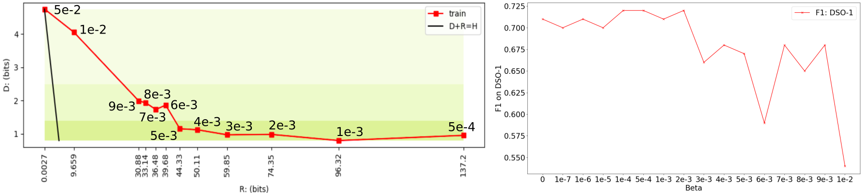
Figure 1: $\beta$ selection from $RD$ curve. Left: $RD$ curve in red, right: F1 metric on DSO-1. Low distortion values are attained for $\beta\leq 5e-3$, while a peak in the F1 is observed from 2e-3 to 1e-4.

6 Conclusion

We presented a novel information theoretic formulation to address the issue of localizing tampered regions (splices) in fake digital images. Using IB, we proposed an efficient variational solution and showed that it outperformed not only the standard expensive numerical method, but also published forensic methods. Our IB formulation was also unique because we used it to learn noise-residual patterns and suppress semantic contents rather than the other way around. Additionally, we demonstrated our method’s potential to detect inpainting operations by recent deep generative methods. Finally, we identified failure cases such as saturated regions for future research directions.

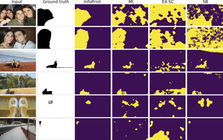
Figure 2: Qualitative results showing the superiority of InfoPrint over published methods.

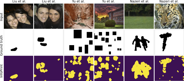
Figure 3: InfoPrint vs inpainting GANs: Liu et al. [26], Yu et al. [37], Nazeri et al. [30].

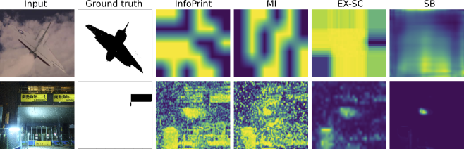
Figure 4: Failure examples. All methods tend to fail when the input image is small: e.g. $335\times 251$ (row-1), or there are saturated regions (row-2). Log-probability maps of proposed methods are shown.

References

- [1] A. Achille and S. Soatto. Information dropout: Learning optimal representations through noisy computation. IEEE Transactions on Pattern Analysis and Machine Intelligence, PP(99), 2018.
- [2] S. Agarwal and H. Farid. Photo forensics from JPEG dimples. In 2017 IEEE Workshop on Information Forensics and Security (WIFS), pages 1–6, 12 2017.
- [3] Alexander Alemi, Ben Poole, Ian Fischer, Joshua Dillon, Rif A. Saurous, and Kevin Murphy. Fixing a broken ELBO. In Proceedings of the 35th International Conference on Machine Learning (ICML), Jul 2018.
- [4] Alexander A. Alemi, Ian Fischer, Joshua V. Dillon, and Kevin Murphy. Deep variational information bottleneck. In International Conference on Learning Representations (ICLR), Apr 2017.
- [5] Anonymous. SpliceRadar: A learned method for blind image forensics. In Supplied as supplementary material, 2019.
- [6] David Barber and Felix V. Agakov. The IM algorithm: A variational approach to information maximization. In NeurIPS, 2003.
- [7] Mauro Barni, Ehsan Nowroozi, and Benedetta Tondi. Higher-order, adversary-aware, double JPEG-detection via selected training on attacked samples. In 25th European Signal Processing Conference (EUSIPCO), pages 281 – 285, 08 2017.
- [8] Mohamed Ishmael Belghazi, Aristide Baratin, Sai Rajeshwar, Sherjil Ozair, Yoshua Bengio, Aaron Courville, and Devon Hjelm. Mutual information neural estimation. In Proceedings of the 35th International Conference on Machine Learning, (ICML), pages 531–540, 10–15 Jul 2018.
- [9] Luca Bondi, Silvia Lameri, David Güera, Paolo Bestagini, Edward Delp, and Stefano Tubaro. Tampering detection and localization through clustering of camera-based CNN features. In The IEEE Conference on Computer Vision and Pattern Recognition (CVPR), pages 1855–1864, 07 2017.
- [10] Christopher P. Burgess, Irina Higgins, Arka Pal, Loic Matthey, Nick Watters, Guillaume Desjardins, and Alexander Lerchner. Understanding disentangling in -VAE. arXiv e-prints, page arXiv:1804.03599, Apr 2018.
- [11] Mo Chen, Jessica Fridrich, Miroslav Goljan, and Jan Lukás. Determining image origin and integrity using sensor noise. Information Forensics and Security, IEEE Transactions on, 3:74 – 90, 04 2008.
- [12] Xi Chen, Yan Duan, Rein Houthooft, John Schulman, Ilya Sutskever, and Pieter Abbeel. InfoGAN: Interpretable representation learning by information maximizing generative adversarial nets. In NeurIPS, 2016.
- [13] D. Cozzolino, G. Poggi, and L. Verdoliva. Splicebuster: A new blind image splicing detector. In 2015 IEEE International Workshop on Information Forensics and Security (WIFS), pages 1–6, 11 2015.
- [14] Davide Cozzolino and Luisa Verdoliva. Noiseprint: a CNN-based camera model fingerprint. arXiv, 2018.
- [15] T. J. d. Carvalho, C. Riess, E. Angelopoulou, H. Pedrini, and A. d. R. Rocha. Exposing digital image forgeries by illumination color classification. IEEE Transactions on Information Forensics and Security, 8(7):1182–1194, 07 2013.
- [16] R Devon Hjelm, Alex Fedorov, Samuel Lavoie-Marchildon, Karan Grewal, Phil Bachman, Adam Trischler, and Yoshua Bengio. Learning deep representations by mutual information estimation and maximization. arXiv e-prints, page arXiv:1808.06670, Aug 2018.
- [17] Ahmet Emir Dirik and Nasir Memon. Image tamper detection based on demosaicing artifacts. In in Proceedings of the 2009 IEEE International Conference on Image Processing (ICIP), 2009.
- [18] Jonathan Fiscus, Haiying Guan, Yooyoung Lee, Amy Yates, Andrew Delgado, Daniel Zhou, David Joy, and August Pereira. The 2017 Nimble Challenge Evaluation: Results and Future Directions, 2017.
- [19] J. Fridrich and J. Kodovsky. Rich models for steganalysis of digital images. IEEE Transactions on Information Forensics and Security, 7(3):868–882, 06 2012.
- [20] Thomas Gloe and Rainer Böhme. The ‘Dresden Image Database’ for benchmarking digital image forensics. In Proceedings of the 25th Symposium On Applied Computing (ACM SAC), volume 2, pages 1585–1591, 2010.
- [21] Ian J. Goodfellow, Jean Pouget-Abadie, Mehdi Mirza, Bing Xu, David Warde-Farley, Sherjil Ozair, Aaron Courville, and Yoshua Bengio. Generative adversarial nets. In NeurIPS, 2014.
- [22] K. He, X. Zhang, S. Ren, and J. Sun. Deep residual learning for image recognition. In The IEEE Conference on Computer Vision and Pattern Recognition (CVPR), pages 770–778, 06 2016.
- [23] Irina Higgins, Loic Matthey, Arka Pal, Christopher Burgess, Xavier Glorot, Matthew Botvinick, Shakir Mohamed, and Alexander Lerchner. -VAE: Learning basic visual concepts with a constrained variational framework. In International Conference on Learning Representations (ICLR), Apr 2017.
- [24] Minyoung Huh, Andrew Liu, Andrew Owens, and Alexei A. Efros. Fighting fake news: Image splice detection via learned self-consistency. In Vittorio Ferrari, Martial Hebert, Cristian Sminchisescu, and Yair Weiss, editors, Proceedings of the European Conference on Computer Vision (ECCV), pages 106–124, Cham, 2018. Springer International Publishing.
- [25] Diederik P. Kingma and Max Welling. Auto-encoding variational bayes. In 2nd International Conference on Learning Representations, (ICLR) 2014, Banff, AB, Canada, April 14-16, 2014, Conference Track Proceedings, 2014.
- [26] Guilin Liu, Fitsum A Reda, Kevin J Shih, Ting-Chun Wang, Andrew Tao, and Bryan Catanzaro. Image inpainting for irregular holes using partial convolutions. In Proceedings of the European Conference on Computer Vision (ECCV), pages 85–100, 2018.
- [27] J. Lukas, J. Fridrich, and M. Goljan. Detecting digital image forgeries using sensor pattern noise - art. no. 60720y. Proceedings of SPIE - The International Society for Optical Engineering, 6072:362–372, 02 2006.
- [28] Babak Mahdian and Stanislav Saic. Using noise inconsistencies for blind image forensics. Image and Vision Computing, 27(10):1497 – 1503, 2009. Special Section: Computer Vision Methods for Ambient Intelligence.
- [29] Owen Mayer and Mathew C. Stamm. Learned forensic source similarity for unknown camera models. In IEEE International Conference on Acoustics, Speech and Signal Processing (ICASSP). IEEE SigPort, 2018.
- [30] Kamyar Nazeri, Eric Ng, Tony Joseph, Faisal Qureshi, and Mehran Ebrahimi. Edgeconnect: Generative image inpainting with adversarial edge learning. arXiv preprint arXiv:1901.00212, 2019.
- [31] N. Otsu. A threshold selection method from gray-level histograms. IEEE Transactions on Systems, Man, and Cybernetics, 9(1):62–66, Jan 1979.
- [32] Xue Bin Peng, Angjoo Kanazawa, Sam Toyer, Pieter Abbeel, and Sergey Levine. Variational Discriminator Bottleneck: Improving Imitation Learning, Inverse RL, and GANs by Constraining Information Flow. In International Conference on Learning Representations (ICLR), May 2019.
- [33] A. C. Popescu and H. Farid. Exposing digital forgeries in color filter array interpolated images. IEEE Transactions on Signal Processing, 53(10):3948–3959, 10 2005.
- [34] Andrew Michael Saxe, Yamini Bansal, Joel Dapello, Madhu Advani, Artemy Kolchinsky, Brendan Daniel Tracey, and David Daniel Cox. On the information bottleneck theory of deep learning. In International Conference on Learning Representations (ICLR), May 2018.
- [35] Ravid Shwartz-Ziv and Naftali Tishby. Opening the Black Box of Deep Neural Networks via Information. arXiv e-prints, page arXiv:1703.00810, Mar 2017.
- [36] Naftali Tishby, Fernando C. Pereira, and William Bialek. The information bottleneck method. In Proc. of the 37-th Annual Allerton Conference on Communication, Control and Computing, pages 368–377, 1999.
- [37] Jiahui Yu, Zhe Lin, Jimei Yang, Xiaohui Shen, Xin Lu, and Thomas S Huang. Generative image inpainting with contextual attention. In Proceedings of the IEEE Conference on Computer Vision and Pattern Recognition (CVPR), pages 5505–5514, 2018.
- [38] Markos Zampoglou, Symeon Papadopoulos, and Ioannis Kompatsiaris. Large-scale evaluation of splicing localization algorithms for web images. Multimedia Tools and Applications, 09 2016.
- [39] Peng Zhou, Xintong Han, Vlad I. Morariu, and Larry S. Davis. Learning rich features for image manipulation detection. In The IEEE Conference on Computer Vision and Pattern Recognition (CVPR), pages 1053–1061, 06 2018.