Semi-Supervised Self-Growing Generative Adversarial Networks for Image Recognition

Abstract

Image recognition is an important topic in computer vision and image processing, and has been mainly addressed by supervised deep learning methods, which need a large set of labeled images to achieve promising performance. However, in most cases, labeled data are expensive or even impossible to obtain, while unlabeled data are readily available from numerous free on-line resources and have been exploited to improve the performance of deep neural networks. To better exploit the power of unlabeled data for image recognition, in this paper, we propose a semi-supervised and generative approach, namely the semi-supervised self-growing generative adversarial network (SGGAN). Label inference is a key step for the success of semi-supervised learning approaches. There are two main problems in label inference: how to measure the confidence of the unlabeled data and how to generalize the classifier. We address these two problems via the generative framework and a novel convolution-block-transformation technique, respectively. To stabilize and speed up the training process of SGGAN, we employ the metric Maximum Mean Discrepancy as the feature matching objective function and achieve larger gain than the standard semi-supervised GANs (SSGANs), narrowing the gap to the supervised methods. Experiments on several benchmark datasets show the effectiveness of the proposed SGGAN on image recognition and facial attribute recognition tasks. By using the training data with only $4\%$ labeled facial attributes, the SGGAN approach can achieve comparable accuracy with leading supervised deep learning methods with all labeled facial attributes.

I Introduction

In the past decade, we have witnessed the increasing interests in the image recognition problem solved by the deep learning approaches [29, 53, 21]. This interest is expanding quickly to many different fields ever since the advent of deep convolution neural networks [29, 53, 17, 21], resulting in many effective approaches in many different computer vision fields [38, 7, 15, 35, 39]. However, despite these exciting progresses, most existing approaches are supervised learning based and largely limited by resorting to huge amounts of data with labels. Labeling these data will incur expensive costs on human labor. To alleviate the dependence of supervised learning approaches on the labeled data, many semi-supervised learning approaches [9, 23, 16, 10, XU2019679] have been developed to exploit the power of the numerous unlabeled data available in free on-line resources for the image recognition problem. On the other hand, with the successes of Deep Convolutional Generative Adversarial Networks (DCGAN) [47] on general pattern recognition tasks, Generative Adversarial Networks (GANs) have been widely applied into unsupervised learning problems [52].

It is well known that the GANs can hardly be trained deeply enough when compared to the other concurrently networks such as ResNet [21]. This is because that the generator of the GANs are usually very shallow and can often drift to “model collapse” (a parameter setting where it always emits the same point), restricting the GANs to grow up to achieve promising performance on large scale datasets such as ImageNet [12]. In this paper, we propose a novel a self-growing GAN (SGGAN) for large scale image recognition tasks. The proposed SGGAN is a united semi-supervised GAN containing three self-growing groups. Each group contains a generator and a discriminator, which are trained at the same time and compete against each other to reach the Nash equilibrium of the game theory through an adversarial objective [17]. The generator is trained to defeat the discriminator by creating virtually realistic images (maximize the loss), and the discriminator is trained to distinguish the images generated by the generator (minimize the loss). Through this min-max game, the loss of generator will become increased while the loss of the discriminator will becomes decreased. Finally, the two losses will become closer to each other, and reach an equilibrium in the end.

In semi-supervised learning (SSL) framework, label inferring is a major challenging to its success. Given an amount of labeled data and a larger amount of unlabeled data, the SSL framework can infer the latent label information of the unlabeled data from the labeled data by considering the structures and distributions of all these data as a whole. In order to guarantee the success of the semi-supervised learning approach, label inference of the unlabeled data is the most significant problem to address. For the labels assigned to the unlabeled data, the false positive rate of the label inference process is more important than the true negative rate for the recognition performance, since false positive labels would add noise into the training data and thus make the training unstable. Therefore, the confidence of the latent labeled data (i.e., unlabeled data with latent labels) should be accurate enough. Moreover, the semi-supervised classifiers may not improve if they perform well on the same types of data. Therefore, the two main obstacles in label inference are: how to measure the confidence of the unlabeled data, and how to generalize the semi-supervised learning classifier. In this paper, we propose to address the first problem through threshold setting techniques [6], in which only the unlabeled data with recognition probability larger than a pre-set threshold will be assigned with a latent label. We solve the second problem by proposing a novel technique named convolution-block-transformation (CBT) proposed by us. In our proposed network, the depth is designed to be deep in order to generalize the classifier since deeper model enables the network to learn more information from the unlabeled data than the shallower one. It is difficult to directly train a deep network in our case, so we propose a simple yet effective convolution block transformation (CBT) technique to transfer weights from a shallower network to a deep one by shortcut and an adaptive scaling layer following the shallower convolution block. We evaluate our method on CIFAR10, SVHN and face attribute recognition dataset, which is more challenging due to complex face variations.

In summary, the major contributions of this paper are summarized as follows:

• We propose an semi-supervised self-growing generative adversarial network (SGGAN) for image recognition problem. We handle the semi-supervised learning problem via label inference to improve the performance of the training network.

• We introduce the minimum mean discrepancy (MMD) as the objective of the feature matching stage to replace the traditional $\ell_{1}$ distance objective. The employed MMD can help to stabilize the training of the proposed SGGAN model, and thus avoid the model collapse pitfall of traditional GANs.

• We propose a novel convolution block transformation (CBT) technique to harmonize the self-growing process of the proposed SGGAN model to address the generalization of its classifier. We prove it is easier to train a model growing from a shallow network to a deep one, and thus achieving better performance.

• We conduct extensive experiments on image and face attribute recognition problems to systematically evaluate our proposed SGGAN model. We demonstrate that MMD and CBT can separately and simultaneously stabilize the training of the proposed SGGAN. When compared with supervised methods, SGGAN can achieves competitive or even higher accuracies on various benchmark datasets when compared with state-of-the-art GAN based approaches such as the Improved GAN [52] and supervised learning networks such as VGG-16 [53] and ResNet-50 [21].

The rest of this paper is organized as follows: In Section II, we briefly reviews related work on semi-supervised learning, generative adversarial networks, the optimization of GAN and face attribute recognition. In Section III, we introduces the architecture of our proposed semi-supervised self-growing generative adversarial network and how to train our SGGAN. Experiments and detailed analysis are introduced in Section IV. Finally, we conclude this paper in Section V.

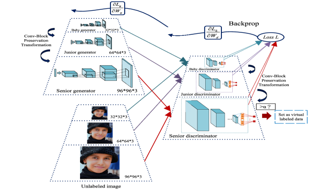
Figure 1: The architecture of our semi-supervised self-growing generative adversarial network (SGGAN). SGGAN starts from the basic baby generator and discriminator, in which the junior and senior generator/discriminator are self-grown from the baby counterparts via our proposed CBT technique.

II Related Work

II-A Semi-Supervised Learning

Semi-supervised algorithm [6] falls between unsupervised learning (e.g., clustering) and supervised learning (e.g., classification or regression) on providing the data labels [75, 73, 67, 66, 68, 65, 61, 63, 62, 64, 1, 36, 70, 69, 72, 71, 22, 59]. Semi-supervised learning [78] contains multiple types of training strategy, such as self-training [49] and co-training [77]. Recently, Zhuang et al. [79] considered the label information in the graph learning stage. Specifically, they enforce to be zero the weight of edges between every two labeled samples from different classes. To make use of the unlabeled data, one simple and effective way is to predict the labels of the unlabeled data by employing the model trained on existing labeled data. Indeed, the premise behind semi-supervised learning is that the learned statistics in the labeled examples contain information which is useful to predict the unknown labels. Self-training [49] is one of the earliest semi-supervised learning strategy using unlabeled data to improve the training of recognition systems. The high confidence that the model predicts against a sample indicates the high probability of correct prediction.

Table I: Architecture of Discriminators.

Baby D	Junior D	Senior D
Input (32$\times$32$\times$3)	Input (128$\times$128$\times$3)	Input (512$\times$512$\times$3)
Conv3-64S1	Conv3-64S1	Conv3-64S1
Conv3-64S1	Conv3-64S1	Conv3-64S1
Conv3-64S2	Conv3-64S2	Conv3-64S2
Conv3-128S2$\times 2$	Conv3-128S2$\times 2$	Conv3-128S2$\times 2$
Conv3-128S1$\times 2$	Conv3-128S1$\times 2$	Conv3-128S1$\times 2$
Conv3-128S1$\times 1$	Conv3-128S1$\times 1$	Conv3-128S1$\times 1$
$-$	Conv3-192S1$\times 2$	Conv3-192S1$\times 2$
$-$	Conv3-192S1$\times 2$	Conv3-192S1$\times 2$
$-$	Conv3-192S2$\times 1$	Conv3-192S2$\times 1$
$-$	$-$	Conv3-256S1$\times 2$
$-$	$-$	Conv3-256S1$\times 2$
$-$	$-$	Conv3-256S2$\times 2$
Dropout(0.5)
Global Average Pooling
FC
softmax

Table II: Architecture of Generators.

Baby G	Junior G	Senior G
Sample 100 number from Uniform Distribution
FC-512*4*4
Reshape-(4,4,512)
Deconv5-256S2	Deconv5-256S2	Deconv5-256S2
Deconv5-128S2	Deconv5-128S2	Deconv5-128S2
Deconv5-128S2	Deconv5-128S2	Deconv5-128S2
-	Deconv5-128S1	Deconv5-128S1
-	Deconv5-128S2	Deconv5-128S2
-	Deconv5-128S2	Deconv5-128S2
-	Deconv5-128S1	Deconv5-128S1
$-$	Deconv5-64S2	Deconv5-64S2
$-$	Deconv5-64S2	Deconv5-64S2
$-$	Deconv5-32S1	Deconv5-32S1
$-$	$-$	Deconv5-32S2
$-$	$-$	Deconv5-32S2
Output(32$\times$32$\times$3)	Output(128$\times$128$\times$3)	Output(512$\times$512$\times$3)
Tanh Activation

II-B Generative Adversarial Networks

The training objective of GANs is to find a Nash equilibrium between the discriminative and generator networks by a min-max game. Denote by the generative network in GAN by $G$ and the discriminative network in GAN by $D$. The purpose of the $G$ network is to generate virtually realistic images and the purpose of the $D$ network is to distinguish between the virtually generated and realistic unlabeled images through the min-max optimization problem. As described in the original paper [17], the purpose of the generative modeling is to find a probabilistic model $Q$ that matches the true data distribution $P$. The training of GAN can be interpreted as minimizing the Jensen-Shannon divergence under some ideal conditions. The Jensen-Shannon divergence is not measured by the K-L divergence between $P$ and $Q$, i.e., $KL[P\|Q]$ or $KL[Q\|P]$, but is between the two extreme cases $KL[P\|Q]$ and $KL[Q\|P]$. And this property of the Jensen-Shannon divergence can push the generator to generate better samples than other methods [17]. Actually, Nash equilibrium is difficult to achieve and the assumptions behind GANs maybe too strong to perfectly match the cases in real-world applications. In the work of DCGAN [47], there are several techniques proposed to stabilize the training of the GANs, i.e., using leaky-ReLUs and batch normalization for the training of the discriminator network, and convolution with stride $2$ instead of max-pooling layers for the training of the generator network. These techniques work very well and have become a standard setup in recent GAN based approaches. Recently, Wasserstein distance [2] is introduced with theoretically proved effectiveness as the objective of the generative model to stabilize the training process of GAN. The main advantage of Wasserstein distance based GAN frameworks is that this distance can guarantee great stability for training the generative model, which is not limited to the DCGAN approach.

Existing GAN based approaches can be categorized into two types from the perspective of their motivations. The first type is the divergence minimization based approaches [47], which mainly focus on designing an effective generator network to produce virtually realistic images, and treat the discriminator network as an auxiliary model. And the second type is the contrast function based approaches [52], which attempt to enhance the discriminating power of the discriminator by simulating a large amount of fake samples. Our work can be categorized into the second type of approaches.

II-C GAN based semi-supervised learning

Donahue et al. [13] introduced an adversarial formulation with a third component, which they call the “encoder”. While the generator maps a simple latent distribution to data space, the encoder attempts to encode real data to some latent space. They show that this encoder is capable of learning to invert the generator, and can be used as a feature for a supervised training. On the autoregressive side, Dai et al.  [11] explored the idea of first “pretraining” a sequence model to perform a task on unlabeled text data. These pretrained weights are then used to train supervised models for text classification. Their results show improved learning stability and model generalization. Radford et al. [46] trained an mLSTM RNN on Amazon reviews to learn a language model and then used its internal cell state from the last time step as features for the subsequent supervised task of sentiment analysis of Amazon reviews. This enabled the authors to match the state-of-the-art in their sentiment analysis dataset with significantly less labeled data and to surpass it with the fully-supervised learning. Recently, Salimans, et al. [52] proposed a way to utilize GANs for a classification task with $k$ classes. Specifically, they propose an extension to the vanilla GAN where the labeled dataset is augmented with samples from the generator. The discriminator is also modified to predict $(k+1)$th classes: the original $k$ classes and a new class for fake (generated) data. In a sense this helps the discriminative model by augmenting a smaller labeled dataset with larger unlabeled set of real examples and generated samples.

II-D Face Attribute Recognition

Face attribute recognition in the wild is a challenging problem due to complex face variations such as varying lightings, scales, and occlusions, etc. Traditionally, previous attribute recognition approaches [4, 5, 31] focus on extracting effective hand-crafted low-level features, e.g., edges, HSV, and gradients, etc, from the detected faces. Then the extracted features are fed into a standard classifier, such as SVM [55] and random forest [37]. For instance, the authors of FaceTracer [30] split the whole face region into multiple sub-regions, extracted multiple types of features for each region, and train a SVM classifier on the concatenated features. Recently, deep learning (especially CNN based) methods [29] have achieved great success in face attribute recognition due to their ability to learn discriminative features from huge amount of labeled data. The authors in [40] applied two CNNs (ANet and LNet) to the face attribute recognition task, on which the LNet is trained to locate the entire face region and the ANet is trained to extract high-level face representation. Finally, the extracted features are fed into a SVM classifier to produce the final recognition results. In [50], the authors proposed a mixed objective to optimize $40$ face attributes together in a single CNN with $138$ million network parameters. However, these supervised deep learning methods are limited by largely depending on huge amount of labeled training data, which is very costly in real-world applications. This motivates us to utilize the large amount of freely available unlabeled data for the face attribute recognition in a semi-supervised manner.

III Semi-Supervised Self-Growing Generative Adversarial Network

In this section, we first reveal the mechanism of the proposed semi-supervised self-growing generative adversarial network (SGGAN) by presenting its architecture in details. Then the convolution block transformation strategy for network self-growing is illustrated. Finally, we introduce the MMD as an effective metric to stabilize the training of our model.

III-A Architecture of SGGAN

The flowchart of the proposed SGGAN is illustrated in Figure 1. Our SGGAN network includes a group of GANs, in which the junior generator or discriminator grows from corresponding baby counterpart, and the senior generator or discriminator grows from corresponding junior counterpart. The detailed description of the structures of three generators and three discriminators are listed in Table II and  II, respectively. The convolutional layer parameters are denoted as “(convolution type)(kernel size)-(number of channels)-S(stride)”. The activation functions we employed for the generator and discriminator are ReLU and Leaky-ReLU, respectively. Batch normalization is used after each convolution layer. The self growing process will be discussed in the next subsection. In the whole network, the fundamental component is named as the GAN cell, which is composed of a generator network and a discriminator network.

In the GAN cell, the discriminator is deeper and sometimes has more filters per layer than the corresponding generator. The reason is that it is important for the discriminator to be able to correctly estimate the ratio between the true data density and generated data density, but it may also be an artifact of the “mode collapse” since the generator tends not to use its full capacity with current training methods [18]. We introduce each component of the proposed SGGAN model as follows.

III-A1 Generator

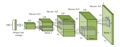
Figure 2: The detailed architecture of Baby Generator.

The generator takes as input a random vector $z$ (drawn from a Gaussian distribution). After reshaping $z$ into a $4$-dimensional shape, it is fed to the generator that starts with a series of upsampling layers. Each upsampling layer represents a transposed convolution operation with a stride of $2$. The transposed convolution work by swapping the forward and backward passes of a convolution. The upsampling layers go from deep and narrow layers to wider and shallower ones. The stride of a transposed convolution operation defines the upsampling factor of the output layer. With the stride of $2$, the size of output features will be twice that of the input layer. After each transposed convolution operation, the reshaped $z$ becomes wider and shallower. All transposed convolutions use a $5\times 5$ kernel with depths reducing from $512$ to $3$, which indicating a RGB color image. The output of the final layer is a $H\times W\times 3$ tensor, squashed between values of $-1$ and $1$ through the Hyperbolic Tangent ($tanh$) function. The shape of the final output is defined by the size of the training image. Specifically, if we train the generator on the SVHN dataset [45], it will produce an image of size $32\times 32\times 3$.

III-A2 Discriminator

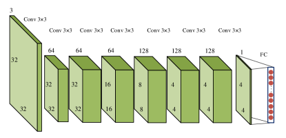
Figure 3: The detailed architecture of Baby Discriminator.

The baby discriminator has $9$ CNN layers with Batch Normalization [25], followed by Leaky-ReLU activation function. It is the same with the deep neural networks used for image recognition [57], object detection [58], and image segmentation [44], etc. The difference is that the Leaky-ReLU [60] is used in our discriminator instead of the regular ReLU [20]. The reason we employ Leaky-ReLU instead of the regular ReLU is that, the regular ReLU function will truncate the negative values to $0$, which will block the gradients to flow through the generative networks. Instead of forcing the negative part to be $0$, the Leaky-ReLU allows a small negative value to pass through the activation layer. Theoretically, Leaky-ReLU represents an attempt to solve the dying ReLU problem [42]. This situation occurs when the neurons do not move in a state in which ReLU units always output $0$s for all inputs. For these scenarios, the gradients do not flow back through the network. This problem is especially important for GAN since the only way the generator learns is by receiving the gradients from the discriminator.

Our baby discriminator takes into a $32\times 32\times 3$ image tensor as input. Being opposite to the generator, the discriminator contains a series of convolutions with a stride of $2$. Each layer reduces the spatial dimensions of feature vector by reducing its size by half, along with doubling the number of learned filters. Given the training data from $k$ classes, the discriminator will output $(k+1)$ neurons to represent these $k$ classes, where the $(k+1)$th class demonstrates the generated images. We employ the softmax activation function as the output of the final layer to generate the confidence for samples from each class. When the discriminator captures the difference between the generated image and realistic image, it will send a signal to the generator counterpart. This signal is the gradient that flows backward from the discriminator to the generator. Once receiving this signal, the generator is able to adjust its parameters accordingly to generate latent data whose distribution is closer to the true data distribution than the previous generated ones. In the final stage, the generator will produce data as good as that the discriminator hardly distinguishes them apart.

III-A3 Label inference by discriminator

The latent labels of our unlabeled images are firstly created via the baby discriminator, and then updated by the junior discriminator. The self-training approaches usually needs a threshold value to infer the latent labels. The threshold value of the confidence is determined on the validation dataset of CelebA dataset [40]; we set the threshold value as $0.98$ in our experiments. In this way, we can utilize more unlabeled images, and hence train deeper neural networks for better recognition performance.

III-B Self-Growing Network

In this section, we propose a convolution block transformation (CBT) technique to transform an existing network into a deeper one. Our idea is motivated by the Net2Net model [8]. In Net2Net, Chen et al. proposed to initialize a bigger model using the weights of a smaller model. However, they only initialize the weights of one layer in each cycle, and this operation has difficulties with the batch normalization (BN) layer. This is because that the BN layer requires running forward inference on the training data to calculate the mean and variance of activation function, which are then used to set the output scale and bias of the BN layer to disentangle the normalization of the statistics of this layer.

In Figure 4, we show the flowchart of the proposed CBT technique. With the help of CBT, to train a deeper model, we initialize a newly added convolution block (instead of a single layer) with Gaussian noise to break symmetry and add identity shortcut to preserve the potential ability of shallow model. As one can see in Figure 4, the weights of the shallow network are transferred to a consistent block of the deeper network. Some new convolution layers are added to the top of the shallow network. The output values of the newly added convolution block are scaled by an adaptive scaling layer. The adaptive layer is defined by the function $w(t)=1-e^{-t}$, where $t$ denotes the number of total iterations in one epoch divided by current iteration number. The adaptive scaled output is added with that of the shallow layer. Finally, the added results are fed into a global average pooling (GAP) layer (for more details about GAP, please refer to the Section III-E). Here, we call the up-described operator as the convolution block transformation (CBT). Along with the training, the function $w(t)$ for the adaptive layer will gradually approach to $1$ and the newly added convolution block will becomes a part of the original shallow net.

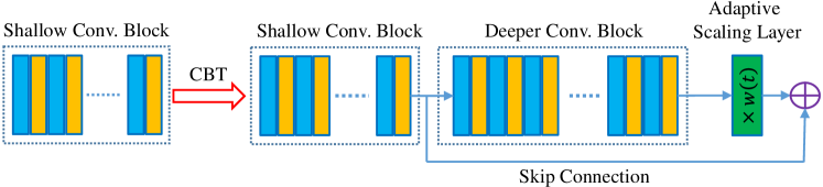
Figure 4: Convolution Block Transformation (CBT) transfers weights of shallow network to the deeper one.

III-C Feature Matching

Generative Adversarial Networks (GANs) are difficult to train since the generator is easy to collapse [18] (we call it the “model collapse” phenomenon). In [52], in order to avoid mode collapse, Salimans et al. proposed the feature matching technique to improve the stability in training the GANs by employing a new objective for the generator. Instead of maximizing the output of the discriminator as the regular GAN training does, the feature matching requires the generator to create latent data that matches the statistics of the realistic data in the feature level of the discriminator network. Consequently, the generator updates its parameters by matching the expectation of the features on the next of the final layer of the discriminator network, which is the output of Global Average Pooling (GAP) layer in our case. This is a natural choice of statistics for the generator to match. Let $f(x)$ denote activations after GAP layer of the discriminator, the feature matching objective for the generator is proposed by [52] and defined by an $\ell_{1}$ distance as $||E_{x\in p_{data}}f(x)-E_{z\in p_{z}(z)}f(G(z))||_{1}$. In practice, we found that the above mentioned $\ell_{1}$ distance produces similar results with $\ell_{2}$ distance. The authors in [14] proved that the maximum mean discrepancy (MMD) using Gaussian kernels could match all moment’s mean, including the $\ell_{1}$ and $\ell_{2}$ distances between the generated features and unlabeled images. Therefore, in this work we employ the MMD metric as the feature matching objective to measure the distance between the features of generated images and unlabeled images. Then, we require generator to match the all levels statistics features of realistic data:

$$\begin{split}\textrm{MMD}(\mathcal{F},p_{data},p_{z})&=\sup_{f\in\mathcal{F}}(\mathbb{E}_{x\sim p_{data}}[f(x)\\ &-\mathbb{E}_{z\sim p_{z}}[f(G(z))]),\end{split}$$ (1)

where $\mathcal{F}$ is a set of functions. When $\mathcal{F}$ is in a reproducing kernel Hilbert space (RKHS), the function approaching the supremum can be derived analytically and is called the witness function

$$f(x)=\mathbb{E}_{x\sim p_{data}}[\mathcal{K}(x,G(z))]-\mathbb{E}_{z\sim p_{z}}[\mathcal{K}(x,G(z))],$$ (2)

where $\mathcal{K}$ is the kernel of the RKHS. Here, we assume $\mathcal{K}$ is measurable and bounded. Then we substitute (2) into (1) and yield:

$$\begin{split}\textrm{MMD}^{2}(\mathcal{F},p_{data},p_{z})&=\mathbb{E}_{x,x^{\prime}\sim p_{data}}[\mathcal{K}(x,x^{\prime})]\\ &-2\mathbb{E}_{x\sim p_{data},z\sim p_{z}}[\mathcal{K}(x,G(z))]\\ &+\mathbb{E}_{z,z\sim p_{z}}[\mathcal{K}(G(z),G(z^{\prime}))].\end{split}$$ (3)

This expression only involves expectations of the kernel $\mathcal{K}$, which can be approximated by:

$$\begin{split}\textrm{MMD}_{sample}^{2}(\mathcal{F},p_{data},p_{z})&=\frac{1}{m^{2}}\sum_{i,j=1}^{m}\mathcal{K}(x_{i},x_{j})\\ -\frac{2}{mn}\sum_{i,j=1}^{m,n}\mathcal{K}(x_{i},G(z_{j}))&+\frac{1}{n^{2}}\sum_{i,j=1}^{n}\mathcal{K}(G(z_{i}),G(z_{j}))\end{split}$$ (4)

The MMD metric also depends on the choice of the kernel. We choose the inner product kernel for simplicity.

Algorithm 1 Training of SGGAN.

1:for $e=1,\ldots,epoches$ do

2:     for $t=1,\ldots,batches$ do

3:         Generate images by using generator $G$.

4:         Feed generated, unlabeled, and labeled images into discriminator $D$ to obtain $Loss_{d}$.

5:         Compute $\frac{\partial Loss_{d}}{\partial W_{d}}$ and update $W_{d}$ with $W_{g}$ fixed.

6:         Feed unlabeled and generated images into $D$ to compute $Loss_{g}$.

7:         Compute $\frac{\partial Loss_{g}}{\partial W_{G}}$ through $D$ and update $W_{g}$ with $W_{d}$ fixed.

8:  end for      

9:     Inference unlabeled images and create latent-labeled dataset by using discriminator $D$,

10:end for

11:Initialize a deeper model by using CBT preservation technique.

III-D Learning Objective

A key challenging in semi-supervised GANs is how to construct the loss function. For the losses, we find that the cross-entropy with Adam is a good choice for the optimizer. In [52], Salimans et al. introduce an effective strategy to construct the discriminator loss function $Loss_{d}$. They regard the labeled and unlabeled data as one of $k$ classes and then classify the latently generated data into the $(k+1)$-th class. In this way, $Loss_{d}$ can be defined as follows:

$$Loss_{d}= -\log(\frac{1}{\sum_{i=1}^{m}e^{g_{i}}+1})-\sum_{i=1}^{m}label_{i}\times\log(x_{i})$$ (5)

$$-\log(\frac{\sum_{i=1}^{m}e^{u_{i}}}{\sum_{i=1}^{m}e^{u_{i}}+1})$$

where $-\sum_{i=1}^{m}label_{i}\times\log(x_{i})$, $-\log(\frac{1}{\sum_{i=1}^{m}e^{g_{i}}+1})$, and $-\log(\frac{\sum_{i=1}^{m}e^{u_{i}}}{\sum_{i=1}^{m}e^{u_{i}}+1})$ are the losses related to generated, labeled, and unlabeled images, respectively. Here, $m$ is the batch size, and $x_{i}$, $g_{i}$, $u_{i}$ represent the output (before softmax activation) of the labeled, generated, and unlabeled images, respectively. During the training of the generator, a simple feature matching method is introduced to measure the dissimilarity between two distributions of realistic and latently generated data as described in [52]. Motivated by the effectiveness of the maximum mean discrepancy (MMD) [19, 14], in the proposed SGGAN we utilize MMD metric instead of the $\ell_{1}$ to measure the dissimilarity between latently generated data and the realistic data.

III-E Training

A complete cycle of training the proposed SGGAN contains three iterative steps: 1) train the generator $G$ and discriminator $D$ on the labeled and unlabeled pool. Here, we employ the MMD metric for the updating of the weights of generator $G$; 2) apply the discriminator $D$ to predict the unlabeled pool, and then assign the most confident samples of all the $k$ classes to the labeled pool; 3) self-grow the discriminator $D$ and generator $G$ to be deeper and more powerful. The overall procedures of training the proposed SGGAN is summarized in Algorithm 1.

III-E1 Pre-Training

The purpose of pre-training is to train the initial baby GAN cell. Inspired by the feature matching techniques introduced in the Improved GAN [52], the process of pre-training could solve the problems in training the discriminator. After this stage, we have a baby discriminator which achieves an accuracy of over $80\%$ on the testing set of the CelebA dataset [40]. To this end, we can make use of the trained baby discriminator to infer the latent labels from the unlabeled images. We use Adam with initializing learning rate of $0.01$ to train both the generator $G$ and the discriminator $D$. The weights of baby generator and baby discriminator are initialized by using Xavier’s method [56]. In all experiments, the pixel values of the images are normalized to $[-1,1]$.

III-E2 Label Inference

As we mentioned in Section I, inferring the latent labels of the unlabeled images is the most significant step in training semi-supervised learning models. One typical way to obtain the latent labels of unlabeled data is to hypothesize that the labels predicted by the initial classifier is credible. Under this circumstance, the label inference problem is tackled. However, there are two issues in this approach. The first one is that the initial classifier can be inaccurate towards unlabeled data, and leading wrong absorption of inaccurate data and thus assimilating noise into the training data. The second one is that as the initial classifier does well on the same class of data, adding this type of unlabeled data as latently labeled samples may make the classifier only memorize this specific type of data and cannot be generalized to other data types. How to solve these two issues is crucial to the success of a semi-supervised self-growing network.

For the first issue, we can largely weaken its impact by only selecting the images in the unlabeled pool which have larger recognition probability than a pre-set threshold value $\alpha$, which can be determined by performing recognition experiments on the validation set of benchmark datasets (please refer to the experimental section for more details) through grid search strategy. In this work, we set $\alpha=0.98$. For the second issue, we initialize the junior network from the trained baby counterpart by introducing the proposed CBT preservation technique, and generalize the representational power of the classifier, accordingly. Comparing to the than the shallower network, a deeper network can potentially learn additional useful information from the latent labeled data. The improving performance of the Alexnet [29] to the VGG [53], and finally to the ResNet [21], all demonstrates the great successes in the ILSVRC [51] challenge on the Imagenet Dataset [12]. For example, VGG [53] uses $3\times 3$ convolution to achieve deeper architecture and ResNet [21] treats convolution added with shortcut as a basic unit and repeats that unit until the depth limit of the network is reached. Going deeper can really improve the capacity of network considerably. As the model grows up stronger (deeper), the network can learn useful information not only on labeled images, but also on the latently labeled images.

IV Experiments

In this section, we first evaluate the proposed semi-supervised self-growing GAN (SGGAN) approach and justify the effectiveness of each component in the SGGAN approach. Then we compare SGGAN with other state-of-the-art semi-supervised GAN based approaches on image recognition problem on two widely employed datasets. To demonstrate the broad applicability of the proposed SGGAN approach, we also compare it with the leading supervised deep learning approaches on two commonly used datasets for face attribute recognition.

IV-A Dataset Description

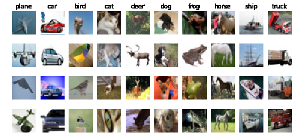
Figure 5: Samples from the CIFAR-10 dataset [28].

Image Recognition Datasets. In this section, we compare the proposed SGGAN approach with state-of-the-art semi-supervised GAN based methods by using the widely used CIFAR-10 dataset [28] and the Street View House Numbers (SVHN) dataset [45].

The CIFAR10 dataset [28] is introduced by A. Krizhevsky and G. Hinton in 2009, and has been a benchmark dataset for image classification problem ever since. This dataset contains $60,000$ color images of size $32\times 32$ in 10 classes (i.e., airplane, automobile, bird, cat, deer, dog, frog, horse, ship, and truck). Some samples of this dataset are shown in Figure 5. Each class includes $6,000$ images, of which $5,000$ images are used for training and $1,000$ images are used for testing. It is a widely used dataset for evaluating both supervised and semi-supervised learning methods on the image recognition problem. We follow the same experimental setting as the previous work such as [52], in which only $100$, $200$, $400$ and $800$ samples along with their labels for each class are randomly selected as the training data for semi-supervised learning.

The SVHN dataset [45] is a real-world image dataset for digit recognition problem. It is similar in flavor to the MNIST dataset [33], but serves with a harder and real-world problem in the wild. This dataset contains over $600,000$ color digit images coming from the house numbers in Google Street View images. Some samples are listed in Figure 6. Among these images, there are $73,257$ images in the training set, $26,032$ images in the testing set. Following the experimental settings as described in [52], in which only $50$, $100$ and $200$ samples along with their labels for each class are selected as the training data for semi-supervised learning.

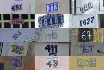
Figure 6: Samples from the SVHN dataset [45].

Facial Attribute Recognition Datasets. We also compare the proposed SGGAN approach with the leading supervised deep learning methods on facial attribute recognition problem with the CelebFaces Attributes Dataset (CelebA) dataset [40] and the Labeled Faces in the Wild-a (LFW-a) dataset [24].

The CelebA dataset [40] is a large-scale face attributes dataset, which contains $202,599$ face images of $10,177$ identities in the wild, each of which includes $5$ landmark locations and $40$ binary attributes annotations. Among the $202,599$ face images in total, $19,962$ images are used as the testing set and the others are used as the training and validation set, respectively. In this article, we randomly select a small set of images as the training set and the others as the testing set.

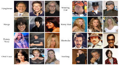
Figure 7: Samples from CelebA dataset [40].

The LFWA dataset [24] has $13,233$ images of $5,749$ identities. Following the experimental settings as the previous work [40], we employ $6,263$ images of $2,749$ peoples as the training set and the other $6,880$ images of $3,000$ peoples as the testing set. When we train the SGGAN model, the labeled images are randomly selected from the training set, and the final results on testing error are averaged by $10$ independent runnings. For the CelebA dataset [40], the prediction threshold $\alpha$ is choose on the validation set.

In all these datasets (except the LFWA dataset [24]), we train the model on the training set and select the model trained with the lowest recognition error on the validation set, and report the testing error with the selected training model accordingly. For the LFWA dataset [24], we follow the experimental settings as described in [40].

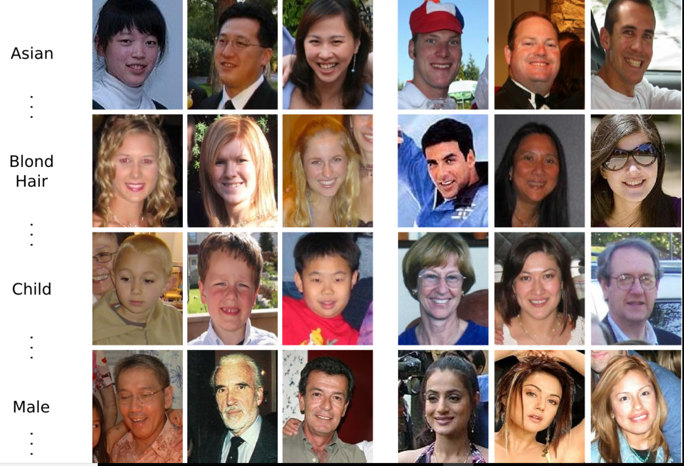
Figure 8: Samples from LFWA dataset [24].

IV-B Ablation Study

In this section, we justify the influence of different components in our proposed SGGAN approach on the performance of recognition errors. The aspects we investigate here include the network self-growing route, the objective function of the feature matching, the generated samples, and the comparison with transfer learning approaches, etc. All these study is evaluated on the training set of the CelebA dataset [40].

Network Self-Growing Route. In our SGGAN model, the model is designed to “grow up” from a small one to a big one. However, how to decide the route for our SGGAN model to achieve better performance (i.e., lower recognition error) is still a big problem. The routes for the model to “grow up” can be very different. For example, the model can be directly grow from a baby model to a junior model, or from a baby model to a senior model, or from a baby model to a junior model and finally to a senior model, etc. To th is end, we design a series of experiment to validate the most suitable “grow up” route for the proposed SGGAN model.

We compare the proposed SGGAN model with different routes of “grow up” on the CelebA dataset [40]. The comparison is performed by using the “gender” attribute of $800$ labeled images. The experimental routes are summarized in the first three rows of the Table III, while symbol “$\surd$” indicates that the corresponding baby/junior/senior model is employed as a part of the whole training model and “$-$” indicates that the we skip the corresponding model. The order in models with three models is to train the whole model from baby one, junior one, to the senior one. From the last row of the Table III, one can see that the SGGAN model with the route of “grow up” along all the three models can achieve higher accuracy than with the other routes. Besides, the SGGAN model “grow up” with two models can achieve better performance than the SGGAN model with only one baby/junior/senior model. Similar findings can be found in the experiments on other attributes of the CelebA dataset [40] as well as on other datasets such as LFWA [24]. These results demonstrate that the network self-growing strategy can effectively improve the image recognition accuracy over the one with fixed single model. Specifically, using all these three models can significantly improve the recognition accuracy of the SGGAN model with only single individual baby/junior/senior network.

Table III: The accuracy (%) of the proposed SGGAN network with different self-growing routes by using the “gender” attribute in the CelebA dataset [40].

Baby	$\surd$	$-$	$-$	$\surd$	$\surd$	$-$	$\surd$
Junior	$-$	$\surd$	$-$	$\surd$	$-$	$\surd$	$\surd$
Senior	$-$	$-$	$\surd$	$-$	$\surd$	$\surd$	$\surd$
Accuracy	80.2	85.1	84.6	86.7	88.5	89.1	89.6

Objective of Feature Matching. The work of Wasserstein GAN [3] discusses different distances between distributions adopted by existing generative adversarial algorithms, and show many of them are discontinuous, such as Jensen-Shannon divergence [17] and Total Variation [76], except for Wasserstein distance. The discontinuity makes the gradient descent infeasible for training. Consequently,  [34] show Wasserstein GAN [3] is a special case of the MMD, and hence MMD also has the advantages of being continuous and differentiable. We adopt the powerful MMD metric to our work to stabilize the training of generator.

We compare the different objective of the feature matching step, i.e., the Maximum Mean Discrepancy (MMD) and the $\ell_{1}$ distance as we have mentioned in Section II. Since the model collapse is a fundamental problem in the training of GAN, we use MMD to stabilize the GAN. The results are shown in Figure 9, from which one can see that the generator trained with the MMD objective can achieve lower training loss than that trained with $\ell_{1}$ distance after several epochs. This demonstrates that MMD is more suitable than the $\ell_{1}$ distance to be the loss objective function during the training of the generator in GAN.

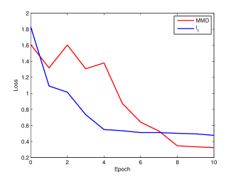
Figure 9: The loss function of the SGGAN model trained with MMD v.s. with $l_{1}$ distance as the objective of feature matching.

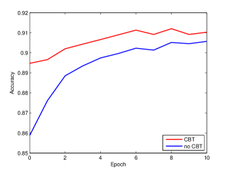
Figure 10: The loss function of the SGGAN model trained with the CBT v.s. without CBT during training.

Convolution Block Transformation (CBT). Figure 10 shows that the recognition accuracy (%) of the SGGAN model trained with the CBT technique are consistently higher than the model trained without CBT in different epochs. This demonstrate that CBT is more effective than its counterpart that simply copies the weights in the shallow model and initializes the newly added convolution-block layers randomly. This is due to the reason that the simple “training without CBT” strategy will wreck the weights in the shallow layers of the network. And evidence our proposed CBT technique will make the transfer of weights smoothly and hence preserve the function of shallower model at the beginning of training.

Comparisons with Fine-tuned VGG and ResNet Networks. In order to show the advantages of our algorithm on label effectiveness, we compare our SGGAN model with the state-of-the-art networks such as the VGG-16 network [53] and the ResNet network [21] in the deep learning field. For the two networks, we load the model provided by corresponding authors pre-trained on the ImageNet dataset [12] (which contains 1000 classes with 1.2 million images), and then carefully fine-tune these networks on the training set of the CelebA dataset [40]. The fine-tuning procedure can usually help the original networks yield better performance than training those networks on small dataset directly. The proposed SGGAN model, the pre-trained VGG-16 and Resnet-50 networks are all fine-tuned with different numbers (i.e., 800, 1600, 3200, 4800, 6400, 7200) of labeled images in the CelebA dataset [40] with ”gender” attribute in the comparison experiments. We fine-tune the VGG-16 and ResNet-50 networks in a standard manner as described in corresponding paper. When the training set is of small scale, it is hard to train a very deep network from scratch. And the most frequently employed technique in literature is to fine-tune the off-the-shell networks, such as the famous VGG network [53]. We compare the proposed SGGAN approach with the fine-tuned VGG-16 and ResNet-50 networks with different numbers of labeled training images.

The results on accuracy (%) are listed in Table IV, from which one can see that when the numbers of labeled training images are $800$, $1,600$, $3,200$, and $4,800$, the proposed SGGAN approach can achieve higher recognition accuracies than the fine-tuned VGG-16 and ResNet-50 networks on the CelebA dataset with the “gender” attribute. Similar results can be found when we perform experiments on the other attributes of the CelebA dataset or the other datasets. When the numbers of the training samples increase to $6,400$ and $7,200$, the proposed SGGAN approach obtains slightly inferior (but still comparable) performance to the VGG-16 and ResNet-50 networks. All these results demonstrate the competing ability of the proposed SGGAN approach as a whole system over the leading VGG and ResNet networks on image recognition tasks such as face attribute recognition.

Table IV: Comparison with the VGG-16 and ResNet-50 networks fine-tuned with different numbers of labeled images from the CelebA dataset [40] with the “gender” attribute.

# of Labeled Image	800	1600	3200	4800	6400	7200
VGG16 [53]	89.3	92.4	94.8	95.9	97.6	98.1
resnet50 [21]	88.6	91.9	94.6	96.2	97.8	98.3
SGGAN	89.6	94.3	95.5	96.4	96.8	97.1

IV-C Comparison with state-of-the-art semi-supervised learning approaches on image recognition

IV-C1 Problem Description

Image recognition problem is the task of assigning one label to an input image from a fixed set of categories. It is a fundamental problem in computer vision community. Image recognition has a large variety of practical applications, and is related to many other computer vision tasks such as object detection and segmentation.

IV-C2 Comparison Methods

We compare the proposed SGGAN approach with other competing semi-supervised learning approaches such as the Ladder Network [48], which proposed to train the ladder network simultaneously minimize the sum of supervised and unsupervised cost functions by back-propagation, avoiding the need for layer-wise pre-training. And some leading GANs based approaches such as CatGAN [54], which is based on an objective function that trades-off mutual information between unlabeled examples and their predicted categorical class distribution, against robustness of the classifier to an adversarial generative model. And the Improved GAN [52], which propose a technique called feature matching to address the instability of GANs by specifying a new objective for the generator to prevents it from overtraining on the current discriminator. Instead of directly maximizing the output of the discriminator, the new objective $\ell_{1}$ requires the generator to generate data that matches the statistics of the real data. We compare these competing methods on the CIFAR10 dataset and the SVHN dataset [45].

IV-C3 Results and Discussions

The experimental results are shown in Table V and Table VI. It can be observed from Table V that we achieve competitive results with the state-of-the-art on the two datasets. As the CIFAR10 dataset [28], the SVHN dataset [45] is used for validating semi-supervised learning methods. Table VI shows the testing error for SVHN experiment. One can see that the more labeled samples we use, the better the recognition performance the proposed SGGAN model will be.

Table V: Comparison test error with other semi-supervised learning methods on CIFAR10 dataset. The results are averaged by 10 runs. N/A is not available, which is not report in their papers.

	1000	2000	4000	8000
Ladder network [48]	N/A	N/A	20.4	N/A
CatGAN [54]	N/A	N/A	19.58	N/A
Improved GANs [52]	21.83	19.61	18.63	17.72
SGGAN	20.04	18.43	15.65	16.51

Table VI: Comparison test error with other semi-supervised learning methods on SVHN dataset. All experiments are averaged by $10$ runs.

	500	1000	2000
DGN [26]	36.02	N/A	N/A
Virtual Adversarial [43]	24.63	N/A	N/A
Auxiliary Deep Generative Model [41]	22.86	N/A	N/A
Skip Deep Generative Model [41]	16.61	N/A	N/A
Improved GANs [52]	18.44	8.11	6.16
SGGAN	17.31	6.53	5.13

IV-D Comparisons with supervised learning approaches on face attribute recognition

Table VII: Comparison with supervised learning methods.

		5 o Clock Shadow	Arched Eyebrows	Attractive	Bags Under Eyes	Bald	Bangs	Big Lips	Big Nose	Black Hair	Blond Hair	Blurry	Brown Hair	Bushy Eyebrows	Chubby	Double Chin	Eyeglasses	Goatee	Gray Hair	Heavy Makeup	H. Cheekbones	Male
CelebA	Face Tracer	85	76	78	76	89	88	64	74	70	80	81	60	80	86	88	98	93	90	85	84	91
	PANDA-w	82	73	77	71	92	89	61	70	74	81	77	69	76	82	85	94	86	88	84	80	93
	LNet+ANet(w/o)	88	74	77	73	95	92	66	75	84	91	80	78	85	86	88	96	92	93	85	84	94
	LNet+ANet	91	79	81	79	98	95	68	78	88	95	84	80	90	91	92	99	95	97	90	87	98
	Virtual GAN	84	73	75	71	92	90	62	74	80	90	77	76	82	85	89	92	88	91	85	80	91
	Auxiliary GAN	85	73	75	74	93	91	63	75	83	91	80	77	83	84	90	93	91	90	86	83	92
	Cat GAN	87	72	76	72	93	92	62	77	81	91	78	75	85	86	90	93	89	91	84	83	93
	Skip GAN	88	75	77	75	96	92	64	78	84	92	81	78	86	87	91	96	92	93	87	84	95
	Improved GAN	87	76	78	76	95	91	65	79	85	91	82	79	87	88	91	95	90	92	88	86	93
	SGGAN	90	77	79	77	98	94	66	80	86	94	83	80	88	89	93	98	94	95	89	86	97
LFWA	FaceTracer	70	67	71	65	77	72	68	73	76	88	73	62	67	67	70	90	69	78	88	77	84
	PANDA-w	64	63	70	63	82	79	64	71	78	87	70	65	63	65	64	84	65	77	86	75	86
	LNets+ANet(w/o)	81	78	80	79	83	84	72	76	86	94	70	73	79	70	74	92	75	81	91	83	91
	LNets+ANet	84	82	83	83	88	88	75	81	90	97	74	77	82	73	78	95	78	84	95	88	94
	Virtual GAN	80	79	77	81	82	81	71	77	84	91	73	74	78	70	74	89	76	80	89	84	88
	Auxiliary GAN	81	80	78	82	83	82	72	78	85	92	74	75	79	71	75	90	77	81	90	85	89
	Cat GAN	80	81	79	81	82	83	73	79	86	91	75	76	80	73	76	89	79	82	89	83	87
	Skip GAN	82	83	81	83	86	83	73	81	88	93	75	78	82	72	78	91	90	82	93	80	90
	Improved GAN	83	82	80	84	85	84	74	80	87	94	76	77	81	73	77	92	79	83	92	87	91
	SGGAN	85	84	82	86	87	86	76	82	89	96	77	79	83	75	79	94	81	85	94	89	93

		Mouth S. O.	Mustache	Narrow Eyes	No Beard	Oval Face	Pale Skin	Pointy Nose	Receding Hairline	Rosy Cheeks	Sideburns	Smiling	Straight Hair	Wavy Hair	Wearing Earrings	Wear. Hat	Wearing Lipstick	Wearing Necklace	Wearing Necktie	Young	Average
CelebA	Face Tracer	87	91	82	90	64	83	68	76	84	94	89	63	73	73	89	89	68	86	80	81
	PANDA-w	82	83	79	87	62	84	65	82	81	90	89	67	76	72	91	88	67	88	77	79
	LNet+ANet(w/o)	86	91	77	92	63	87	70	85	87	91	88	69	75	78	96	90	68	86	83	83
	LNet+ANet	92	95	81	95	66	91	72	89	90	96	92	73	80	82	99	93	71	93	87	87
	Virtual GAN	86	88	77	88	59	85	68	82	83	89	85	69	73	74	93	87	68	86	82	81
	Auxiliary GAN	87	89	78	89	60	86	69	83	84	90	86	70	74	75	94	88	69	87	83	82
	Cat GAN	88	88	77	88	61	87	68	82	85	91	87	71	75	74	93	87	68	76	84	83
	Skip GAN	89	91	80	91	62	88	71	85	86	92	88	72	76	77	96	90	71	89	85	84
	Improved GAN	90	90	81	90	63	89	72	84	87	91	87	73	77	76	95	91	72	88	84	85
	SGGAN	91	93	82	93	64	90	73	87	88	94	90	74	78	79	98	92	73	91	87	86
LFWA	FaceTracer	77	83	73	69	66	70	74	63	70	71	78	67	62	88	75	87	81	71	80	74
	PANDA-w	74	77	68	63	64	64	68	61	64	68	77	68	63	85	78	83	79	70	76	71
	LNets+ANet(w/o)	78	87	77	75	71	81	76	81	72	72	88	71	73	90	84	92	83	76	82	79
	LNets+ANet	82	92	81	79	74	84	80	85	78	77	91	76	76	94	88	95	88	79	86	84
	Auxiliary GAN	78	86	78	77	71	78	76	82	75	76	85	75	74	88	84	91	85	76	78	80
	Auxiliary GAN	79	87	79	78	72	79	77	83	76	77	86	76	75	89	85	92	86	77	79	81
	Cat GAN	80	88	78	77	73	78	78	82	77	78	85	75	76	88	86	91	87	78	78	81
	Skip GAN	81	89	81	80	74	81	79	85	78	79	88	78	77	91	87	94	88	79	81	83
	Improved GAN	82	88	82	81	73	80	80	84	79	80	87	77	78	90	88	93	89	80	82	83
	SGGAN	83	91	83	82	76	83	81	87	80	81	90	80	79	93	89	96	90	81	83	85

IV-D1 Problem Description

Face attributes recognition is to get descriptive attributes on faces (gender, sex, the presence of sunglasses etc). Kumar et al. [32] first introduced them as mid-level features for face verification [31] and since then have attracted much attention. The recognition of face attributes has an important role in computer vision applications due to their detailed description of human faces. The applications of it include suspect identification [27], face verification [32] and face retrieval [31]. Predicting face attributes in the wild in challenging due to complex face variations. In facial attribute recognition field, labeled data are either expensive or unavailable to obtain. Consequently, the large number of unlabeled face images available on the Internet have attracted increasing interests of researchers to tackle facial attribute recognition problem by semi-supervised learning (SSL) [6] methods.

IV-D2 Comparisons methods

The proposed method is compared with four competitive fully-supervised approaches including FaceTracer [30], PANDA-w [74], LNet+ANet(w/o) and LNet+ANet [74] on the two datasets mentioned above. Compared with the fully-supervised learning methods, our self-growing approach only uses $7200$ labeled images. The LFWA dataset is a standard benchmark for face attribute classification. However, the number of training and validation data of LFWA data set is small, which made it not suitable to our algorithm. So we report two patterns of result on LFWA dataset. The first one uses all the training/validation data in the LFWA dataset and the other uses the data of CelebA as the unlabeled data pool. Our algorithm runs ten times, and we report the average result.

IV-D3 Results and Discussions

The comparison results on CelebA and LFWA datasets are shown in Table VII, from which one can see that the proposed SGGAN approach achieve comparable performance on the recognition accuracy when compared with the state-of-the-art supervised learning based deep learning methods. For example, the proposed SGGAN trained with the MMD objective and the CBT technique (i.e., SGGAN-MMD-CBT) achieves an accuracy of $86.22\%$, which is only slightly inferior to the LNet+ANet methods, but still superior to all the other methods. Note that the proposed SGGAN-MMD-CBT approach achieves such promising performance with only $4\%$ labeled training images.

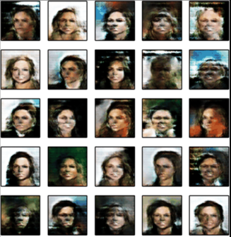
Baby generator

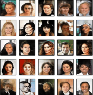
Junior generator

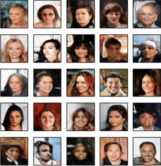
Senior generator

Figure 11: The generated samples of the baby, junior, and senior generators of the proposed SGGAN approach.

IV-E Results on the LFWA dataset using external unlabeled data

The LFWA dataset is a standard benchmark for face attribute recognition. However, the number of training images in LFWA dataset is small ($6,263$ images), which made it not well suitable for our algorithm. In order to achieve semi-supervised learning on LFWA dataset. We use all training images in CelebA dataset as the unlabeled pool for our algorithm to train a SGGAN on LFWA dataset. During training, the labels of CelebA dataset was not used. Table VIII show the results, in the first row of the table, the “LFWA (Outer data)” shows the result of SGGAN using CelebA as the unlabeled pool and “LFWA” is the result of SGGAN only use the images in LFWA. From the table one can see a large number of unlabeled images will improve around $6\%$ points for LFWA dataset. Which also demonstrate the effectiveness of our algorithm for the semi-supervised image recognition tasks.

Table VIII: Recognition accuracy (%) of SGGAN with different component settings on the LFWA dataset [24] by using unlabeled data.

Methods	LFWA (Outer data)	LFWA
Baseline: Feature Matching [52]	81.29	78.56
SGGAN-MMD	83.41	78.53
SGGAN-CBT	84.27	78.57
SGGAN-MMD-CBT	85.32	78.81

IV-F Generated Samples

Feature matching is proved to help the GANs work much better if the goal is to obtain a strong classifier using the approach to semi-supervised learning [52]. It works well for semi-supervised learning approaches. However, the samples generated by the generator during semi-supervised learning using feature matching do not look visually appealing. The reason appears to be that the human visual system is strongly attuned to image statistics that can help infer what class of object an image represents, while it is presumably less sensitive to local statistics that are less important for interpretation of the image. This is supported by the high correlation between the quality reported by human annotators and the Inception score developed in the work [52].

We show the generated samples in Figure 11, from which one can see that the junior generator can produce samples with better image quality than those generated by the baby one, and the senior generator can further enhance the performance of the image quality of the produced samples than those generated by the junior one. This demonstrate that the proposed SGGAN network with “grow up” strategy can indeed make better generation during the training process, and hence implicitly help improve the performance of the GAN model on the recognition tasks.

V Conclusion

In this paper, we propose a simple yet effective semi-supervised self-growing generative adversarial network (SGGAN) for image recognition. We propose a convolution-block-transformation (CBT) preservation technique to promote the network self-growing and obtain deeper network. Meanwhile, we leverage a maximum mean discrepancy (MMD) metric to stabilize and improve the training of SGGAN. The experiments on CIFAR10 and SVHN dataset demonstrate effectiveness our methods. Extensive experiments on the CelebA and LFWA demonstrate the generalization of our method. With only around $4\%$ labeled training data, our SGGAN can achieve comparable performance with the fully-supervised convolutional neural network.

References

- [1] Wangpeng An, Haoqian Wang, Qingyun Sun, Jun Xu, Qionghai Dai, and Lei Zhang. A pid controller approach for stochastic optimization of deep networks. In The IEEE Conference on Computer Vision and Pattern Recognition (CVPR), June 2018.
- [2] Martin Arjovsky and Léon Bottou. Towards principled methods for training generative adversarial networks. In ICLR, 2017.
- [3] Martín Arjovsky, Soumith Chintala, and Léon Bottou. Wasserstein generative adversarial networks. In Proceedings of the 34th International Conference on Machine Learning, ICML 2017, Sydney, NSW, Australia, 6-11 August 2017, pages 214–223, 2017.
- [4] Thomas Berg and Peter Belhumeur. Poof: Part-based one-vs.-one features for fine-grained categorization, face verification, and attribute estimation. In CVPR, 2013.
- [5] Lubomir Bourdev, Subhransu Maji, and Jitendra Malik. Describing people: A poselet-based approach to attribute classification. In ICCV, 2011.
- [6] Olivier Chapelle, Bernhard Schlkopf, and Alexander Zien. Semi-Supervised Learning. The MIT Press, 1st edition, 2010.
- [7] K. Chen and W. Tao. Convolutional regression for visual tracking. IEEE Transactions on Image Processing, PP(99):1–1, 2018.
- [8] Tianqi Chen, Ian J. Goodfellow, and Jonathon Shlens. Net2net: Accelerating learning via knowledge transfer. In ICLR, 2016.
- [9] Yanhua Cheng, Xin Zhao, Rui Cai, Zhiwei Li, Kaiqi Huang, and Yong Rui. Semi-supervised multimodal deep learning for rgb-d object recognition. In IJCAI, 2016.
- [10] Neva Cherniavsky, Ivan Laptev, Josef Sivic, and Andrew Zisserman. Semi-supervised learning of facial attributes in video. In ECCV, 2010.
- [11] Andrew M Dai and Quoc V Le. Semi-supervised sequence learning. In C. Cortes, N. D. Lawrence, D. D. Lee, M. Sugiyama, and R. Garnett, editors, Advances in Neural Information Processing Systems 28, pages 3079–3087. Curran Associates, Inc., 2015.
- [12] J. Deng, W. Dong, R. Socher, L.-J. Li, K. Li, and L. Fei-Fei. ImageNet: A Large-Scale Hierarchical Image Database. In CVPR, 2009.
- [13] Jeff Donahue, Philipp Krähenbühl, and Trevor Darrell. Adversarial feature learning. arXiv preprint arXiv:1605.09782, 2016.
- [14] Gintare Karolina Dziugaite, Daniel M Roy, and Zoubin Ghahramani. Training generative neural networks via maximum mean discrepancy optimization. UAI, 2015.
- [15] Z. Feng, J. Lai, and X. Xie. Learning view-specific deep networks for person re-identification. IEEE Transactions on Image Processing, PP(99):1–1, 2018.
- [16] Yuan Gao, Jiayi Ma, and Alan L. Yuille. Semi-supervised sparse representation based classification for face recognition with insufficient labeled samples. CoRR, abs/1609.03279, 2016.
- [17] Ian Goodfellow, Jean Pouget-Abadie, Mehdi Mirza, Bing Xu, David Warde-Farley, Sherjil Ozair, Aaron Courville, and Yoshua Bengio. Generative adversarial nets. In NIPS, 2014.
- [18] Ian J. Goodfellow. NIPS 2016 tutorial: Generative adversarial networks. CoRR, abs/1701.00160, 2017.
- [19] Arthur Gretton, Karsten M Borgwardt, Malte J Rasch, Bernhard Schölkopf, and Alexander Smola. A kernel two-sample test. Journal of Machine Learning Research, 13(Mar):723–773, 2012.
- [20] Richard HR Hahnloser, Rahul Sarpeshkar, Misha A Mahowald, Rodney J Douglas, and H Sebastian Seung. Digital selection and analogue amplification coexist in a cortex-inspired silicon circuit. Nature, 405(6789):947, 2000.
- [21] Kaiming He, Xiangyu Zhang, Shaoqing Ren, and Jian Sun. Deep residual learning for image recognition. In CVPR, 2016.
- [22] Yingkun Hou, Jun Xu, Guanghai Liu, Li Liu, Fan Zhu, and Ling Shao. Nlh: A blind pixel-level non-local method for real-world image denoising, 2019.
- [23] Guosheng Hu, Xiaojiang Peng, Yongxin Yang, Timothy M. Hospedales, and Jakob Verbeek. Frankenstein: Learning deep face representations using small data. IEEE Trans. Image Processing, 27(1):293–303, 2018.
- [24] Gary B. Huang, Manu Ramesh, Tamara Berg, and Erik Learned-Miller. Labeled faces in the wild: A database for studying face recognition in unconstrained environments. Technical Report 07-49, 2007.
- [25] Sergey Ioffe and Christian Szegedy. Batch normalization: Accelerating deep network training by reducing internal covariate shift. CoRR, abs/1502.03167, 2015.
- [26] Diederik P Kingma, Shakir Mohamed, Danilo Jimenez Rezende, and Max Welling. Semi-supervised learning with deep generative models. In Advances in Neural Information Processing Systems, pages 3581–3589, 2014.
- [27] Brendan F Klare, Scott Klum, Joshua C Klontz, Emma Taborsky, Tayfun Akgul, and Anil K Jain. Suspect identification based on descriptive facial attributes. In IJCB, 2014.
- [28] Alex Krizhevsky. Learning multiple layers of features from tiny images. 2009.
- [29] Alex Krizhevsky, Ilya Sutskever, and Geoffrey E Hinton. Imagenet classification with deep convolutional neural networks. In NIPS, 2012.
- [30] Neeraj Kumar, Peter Belhumeur, and Shree Nayar. Facetracer: A search engine for large collections of images with faces. In ECCV, 2008.
- [31] Neeraj Kumar, Alexander Berg, Peter N Belhumeur, and Shree Nayar. Describable visual attributes for face verification and image search. IEEE Transactions on Pattern Analysis and Machine Intelligence, 33(10):1962–1977, 2011.
- [32] Neeraj Kumar, Alexander C Berg, Peter N Belhumeur, and Shree K Nayar. Attribute and simile classifiers for face verification. In ICCV, 2009.
- [33] Yann LeCun, Léon Bottou, Yoshua Bengio, and Patrick Haffner. Gradient-based learning applied to document recognition. Proceedings of the IEEE, 86(11):2278–2324, 1998.
- [34] Chun-Liang Li, Wei-Cheng Chang, Yu Cheng, Yiming Yang, and Barnabas Poczos. Mmd gan: Towards deeper understanding of moment matching network. In I. Guyon, U. V. Luxburg, S. Bengio, H. Wallach, R. Fergus, S. Vishwanathan, and R. Garnett, editors, Advances in Neural Information Processing Systems 30, pages 2203–2213. Curran Associates, Inc., 2017.
- [35] J. Li, B. Li, J. Xu, R. Xiong, and W. Gao. Fully connected network-based intra prediction for image coding. IEEE Transactions on Image Processing, PP(99):1–1, 2018.
- [36] Zhetong Liang, Jun Xu, David Zhang, Zisheng Cao, and Lei Zhang. A hybrid l1-l0 layer decomposition model for tone mapping. In The IEEE Conference on Computer Vision and Pattern Recognition (CVPR), June 2018.
- [37] Andy Liaw, Matthew Wiener, et al. Classification and regression by randomforest. R news, 2(3):18–22, 2002.
- [38] D. Liu, Z. Wang, Y. Fan, X. Liu, Z. Wang, S. Chang, X. Wang, and T. S. Huang. Learning temporal dynamics for video super-resolution: A deep learning approach. IEEE Transactions on Image Processing, PP(99):1–1, 2018.
- [39] N. Liu and J. Han. A deep spatial contextual long-term recurrent convolutional network for saliency detection. IEEE Transactions on Image Processing, PP(99):1–1, 2018.
- [40] Ziwei Liu, Ping Luo, Xiaogang Wang, and Xiaoou Tang. Deep learning face attributes in the wild. In ICCV, 2015.
- [41] Lars Maaløe, Casper Kaae Sønderby, Søren Kaae Sønderby, and Ole Winther. Auxiliary deep generative models. arXiv preprint arXiv:1602.05473, 2016.
- [42] Andrew L. Maas, Awni Y. Hannun, and Andrew Y. Ng. Rectifier nonlinearities improve neural network acoustic models. 2013.
- [43] Takeru Miyato, Shin-ichi Maeda, Masanori Koyama, Ken Nakae, and Shin Ishii. Distributional smoothing with virtual adversarial training. arXiv preprint arXiv:1507.00677, 2015.
- [44] Jacinto C. Nascimento and Gustavo Carneiro. Deep learning on sparse manifolds for faster object segmentation. IEEE Trans. Image Processing, 26(10):4978–4990, 2017.
- [45] Yuval Netzer, Tao Wang, Adam Coates, Alessandro Bissacco, Bo Wu, and Andrew Y Ng. Reading digits in natural images with unsupervised feature learning. In ICCV workshop, 2011.
- [46] Alec Radford, Rafal Józefowicz, and Ilya Sutskever. Learning to generate reviews and discovering sentiment. CoRR, abs/1704.01444, 2017.
- [47] Alec Radford, Luke Metz, and Soumith Chintala. Unsupervised representation learning with deep convolutional generative adversarial networks. In ICLR, 2016.
- [48] Antti Rasmus, Mathias Berglund, Mikko Honkala, Harri Valpola, and Tapani Raiko. Semi-supervised learning with ladder networks. In NIPS, 2015.
- [49] Chuck Rosenberg, Martial Hebert, and Henry Schneiderman. Semi-supervised self-training of object detection models. 2005.
- [50] Ethan M Rudd, Manuel Günther, and Terrance E Boult. Moon: A mixed objective optimization network for the recognition of facial attributes. In ECCV, 2016.
- [51] Olga Russakovsky, Jia Deng, Hao Su, Jonathan Krause, Sanjeev Satheesh, Sean Ma, Zhiheng Huang, Andrej Karpathy, Aditya Khosla, Michael Bernstein, Alexander C. Berg, and Li Fei-Fei. ImageNet Large Scale Visual Recognition Challenge. IJCV, 115(3):211–252, 2015.
- [52] Tim Salimans, Ian J. Goodfellow, Wojciech Zaremba, Vicki Cheung, Alec Radford, and Xi Chen. Improved techniques for training gans. In NIPS, 2016.
- [53] K. Simonyan and A. Zisserman. Very deep convolutional networks for large-scale image recognition. In ICLR, 2015.
- [54] Jost Tobias Springenberg. Unsupervised and semi-supervised learning with categorical generative adversarial networks. 2016.
- [55] Johan AK Suykens and Joos Vandewalle. Least squares support vector machine classifiers. Neural processing letters, 9(3):293–300, 1999.
- [56] Christian Szegedy, Wei Liu, Yangqing Jia, Pierre Sermanet, Scott Reed, Dragomir Anguelov, Dumitru Erhan, Vincent Vanhoucke, and Andrew Rabinovich. Going deeper with convolutions. In CVPR, 2015.
- [57] Peng Tang, Xinggang Wang, Bin Feng, and Wenyu Liu. Learning multi-instance deep discriminative patterns for image classification. IEEE Trans. Image Processing, 26(7):3385–3396, 2017.
- [58] Wenguan Wang, Jianbing Shen, and Ling Shao. Video salient object detection via fully convolutional networks. IEEE Trans. Image Processing, 27(1):38–49, 2018.
- [59] Ziqin Wang, Jun Xu, Li Liu, Fan Zhu, and Ling Shao. Ranet: Ranking attention network for fast video object segmentation. In The IEEE International Conference on Computer Vision (ICCV), Oct 2019.
- [60] Bing Xu, Naiyan Wang, Tianqi Chen, and Mu Li. Empirical evaluation of rectified activations in convolutional network. CoRR, abs/1505.00853, 2015.
- [61] J. Xu. Nonlocal self-similarity based prior modeling for image denoising. PhD thesis, The Hong Kong Polytechnic University, 2018.
- [62] J. Xu, Y. Huang, L. Liu, F. Zhu, X. Hou, and L. Shao. Noisy-as-clean: Learning unsupervised denoising from the corrupted image, 2019.
- [63] J. Xu, H. Li, Z. Liang, D. Zhang, and L. Zhang. Real-world noisy image denoising: A new benchmark. arXiv:1804.02603, 2018.
- [64] J. Xu, D. Ren, L. Zhang, and D. Zhang. Patch group based bayesian learning for blind image denoising. Asian Conference on Computer Vision Workshop, pages 79–95, 2016.
- [65] J. Xu, L. Zhang, and D. Zhang. External prior guided internal prior learning for real-world noisy image denoising. IEEE Transactions on Image Processing, 27(6):2996–3010, June 2018.
- [66] J. Xu, L. Zhang, and D. Zhang. A trilateral weighted sparse coding scheme for real-world image denoising. In ECCV, 2018.
- [67] J. Xu, L. Zhang, D. Zhang, and X. Feng. Multi-channel weighted nuclear norm minimization for real color image denoising. In ICCV, 2017.
- [68] J. Xu, L. Zhang, W. Zuo, D. Zhang, and X. Feng. Patch group based nonlocal self-similarity prior learning for image denoising. In ICCV, pages 244–252, 2015.
- [69] Jun Xu, Wangpeng An, Lei Zhang, and David Zhang. Sparse, collaborative, or nonnegative representation: Which helps pattern classification? Pattern Recognition, 88:679 – 688, 2019.
- [70] Jun Xu, Kui Xu, Ke Chen, and Jishou Ruan. Reweighted sparse subspace clustering. Computer Vision and Image Understanding, 138(0):25–37, 2015.
- [71] Jun Xu, Mengyang Yu, Li Liu, Fan Zhu, Dongwei Ren, Yingkun Hou, Haoqian Wang, and Ling Shao. Star: A structure and texture aware retinex model, 2019.
- [72] Zhou Xu, Shuai Li, Xiapu Luo, Jin Liu, Tao Zhang, Yutian Tang, Jun Xu, Peipei Yuan, and Jacky Keung. Tstss: A two-stage training subset selection framework for cross version defect prediction. Journal of Systems and Software, 2019.
- [73] Zhou Xu, Shuai Li, Yutian Tang, Xiapu Luo, Tao Zhang, Jin Liu, and Jun Xu. Cross version defect prediction with representative data via sparse subset selection. In Proceedings of the 26th Conference on Program Comprehension, ICPC ’18, pages 132–143. ACM, 2018.
- [74] Ning Zhang, Manohar Paluri, Marc’Aurelio Ranzato, Trevor Darrell, and Lubomir Bourdev. Panda: Pose aligned networks for deep attribute modeling. In CVPR, 2014.
- [75] Yanping Zhang, Jun Xu, Wei Zheng, Chen Zhang, Xingye Qiu, Ke Chen, and Jishou Ruan. newdna-prot: Prediction of dna-binding proteins by employing support vector machine and a comprehensive sequence representation. Computational Biology and Chemistry, 52(0):51–59, 2014.
- [76] Junbo Jake Zhao, Michaël Mathieu, and Yann LeCun. Energy-based generative adversarial network. CoRR, abs/1609.03126, 2016.
- [77] Zhi-Hua Zhou and Ming Li. Semi-supervised regression with co-training. In IJCAI, volume 5, pages 908–913, 2005.
- [78] Xiaojin Zhu and Andrew B Goldberg. Introduction to semi-supervised learning. Synthesis lectures on artificial intelligence and machine learning, 3:1–130, 2009.
- [79] L. Zhuang, Z. Zhou, S. Gao, J. Yin, Z. Lin, and Y. Ma. Label information guided graph construction for semi-supervised learning. IEEE Transactions on Image Processing, 26(9):4182–4192, Sept 2017.