Transcriptional Response of
SK-N-AS Cells to Methamidophos
Extended Version

Abstract

Transcriptomics response of SK-N-AS cells to methamidophos (an acetylcholine esterase inhibitor) exposure was measured at 10 time points between 0.5 and 48 h. The data was analyzed using a combination of traditional statistical methods and novel machine learning algorithms for detecting anomalous behavior and infer causal relations between time profiles. We identified several processes that appeared to be upregulated in cells treated with methamidophos including: unfolded protein response, response to cAMP, calcium ion response, and cell-cell signaling. The data confirmed the expected consequence of acetylcholine buildup. In addition, transcripts with potentially key roles were identified and causal networks relating these transcripts were inferred using two different computational methods: Siamese convolutional networks and time warp causal inference. Two types of anomaly detection algorithms, one based on Autoencoders and the other one based on Generative Adversarial Networks (GANs), were applied to narrow down the set of relevant transcripts.

1 Introduction

Rapid determination of the mechanism of action (MoA) of an unknown or novel xenobiotic (toxin, drug, pathogen) and its consequences is important both scientifically and for biodefense. It is particularly important to develop methods to identify candidates that are independent of existing experimental data, as there may be no such data available.

Time series data generated by omics experimental techniques provides a wealth of data about change in relative concentrations of transcripts, proteins and metabolites. For example, chemically perturbing cells can result in thousands of mRNAs with at least a 2 fold expression change. The challenge is to get the most information purely from the data, before augmenting the conclusions with knowledge from databases and literature. Thus, it is important to consider not only what changes, but how it changes over time, to identify key responders and how they organize into cellular processes.

As part of the DARPA Rapid Threat Assessment project we developed a suite of data analysis methods to identify candidate biological players and processes that make up the cellular response to a challenge. These included traditional statistical analysis, shape/feature analysis, Gaussian process representation, new machine learning algorithms for identifying anomalies and inferring causal relations between time profiles. The algorithms and methods were developed using data from HepG2/C3A cells exposed to a series of different drugs each affecting different known cellular processess. To test the robustness and generality of the analysis methods we selected a different cell type (SK-N-AS human neuroblastoma cells) and toxin (the organophosphate methamidophos). We expected the biological noise to be different in a different cell type. We also expected the timing and organization of response to an organophosphate to be different from the previously tested drugs. This allows checking that parameters chosen for multiple algorithms work in a more general setting. Here we present three analysis algorithms not previously described, and discuss the application of our suite of algorithms to analysis of methamidophos response data.

Methamidophos is a cholinesterase inhibitor. The enzymes acetylcholinesterase (ACHE) and butyrylcholinesterase (BCHE) convert acetylcholine into the inactive metabolites choline and acetate. The result of acetylcholine esterase inhibition in cultured cells is that acetylcholine builds up and continues to bind and activate muscarinic and nicotinic acetylcholine receptors.

Transcriptomic response of SK-N-AS cells to methamidophos exposure was measured at 10 time points between 0.5 and 48 h. The data was analyzed using our suite of algorithms. This lead to multiple classifications of transcripts and groups of transcripts as candidate elements of the methamidophos broader  MoA. GO process term annotations (using UniProt [5] or PatherDB [13]), databases and curated experimental results were used to refine the data analysis and determine possible biological roles of the identified transcripts. Several biological processes were hypothesized as candidate components of the overall mechanism of action, including unfolded protein response, response to cAMP, and calcium ion related processes. The data also shows response to an increase in the second messenger diacylglycerol (DAG) which is consistent with acetylcholine build up. However, the DAG response was not identified by over-expression analysis, partly because of a lack of relevant GO annotations. Transcripts with potentially key roles were identified and causal networks relating responsive transcripts were inferred. Some of the inferred causal edges correspond to known relations, most are novel and more work is needed to understand what they mean.

Plan

In Section 2 we give an overview of the data analysis process and describe the novel classification and causality inference algorithms. The main results of the data analysis are discussed in Section 3. Details of the experiments generating the data are given in Section 4. Section 5 contains some discusion of results, related and future work. The appendix 6 provides some additional data analysis details.

2 Overview of Data Analysis

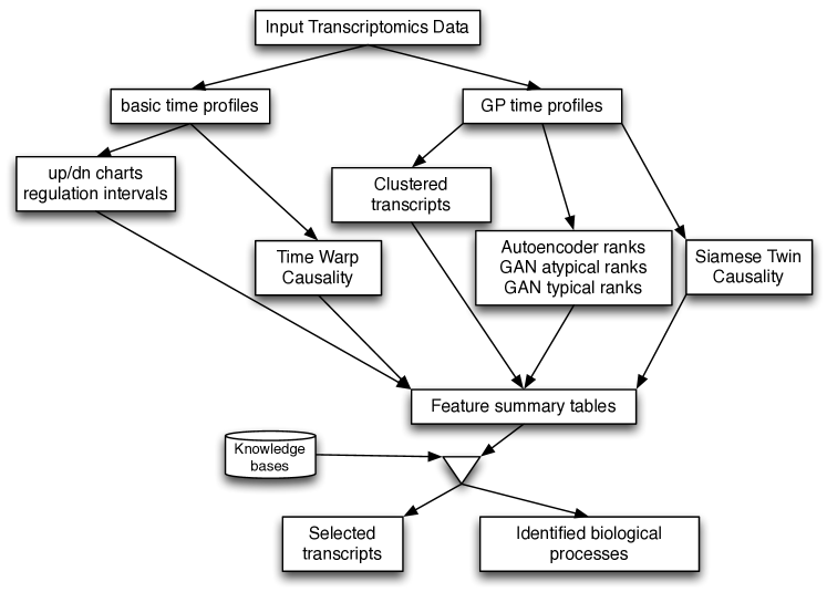
Figure 1: Data analysis schematic

Figure 1 shows a schematic of our data analysis process. The left branch uses log₂ fold change (basic) time profiles derived from the means of the control and treated signals in the usual way. Up/down charts map transcripts to the first time point the log₂ fold change magnitude passes $1$. Regulation intervals delimit times that log₂ fold change stays above $0.75$ or below $-0.75$. The right branch uses time profiles obtained by Gaussian process (GP) modeling [24]. Using these time profiles, transcripts are clustered (k-means using PCA to reduce dimensionality), and ranked by contribution to PCA components and by two machine learning algorithms, one using autoencoder techniques (see [24]) and one using Generative Adversarial Nets (GANs, [6], Section 2.3). Transcripts are ranked highly as anomalies according to how poorly they are reconstructed from the autoencoding, or how unsure the trained GAN discriminator is that the time profile represents a transcript. Transcripts are also given a ‘real/typical’ ranking according to how confident the GAN discriminator is that the time profile represents a transcript. Two algorithms were used to infer potential ‘causal’ edges between time profiles. The Siamese twin causality detection algorithm [19] is based on two Siamese neural networks [3]. One Siamese network is trained to detect undirected causality; the other is trained to detect lag. Lag detection is used to direct the undirected causality edges (see Section 2.4). The Timewarp algorithm operates on basic time profiles and uses a variant of the Needleman-Wunsch alignment algorithm [14] to align time profiles (see Section 2.5). The results of the analyses, along with an indication of satisfaction of several significance filters, are collected in a ‘feature’ table that can be sorted to highlight features of interest. We used the ranking functions and significant change filters to select a set of transcripts, called Top20X, as the starting point for further identification of MoA candidates. We consider two categories: biological processes, individual transcripts. To identify candidate processes we used PatherDB over representation analysis [13] combined with our GO term annotations of k-means clusters [24]. Potentially key transcripts were selected from the Top20X transcripts using a combination of ranking, clustering, and GO annotations.

2.1 The input data

Transcriptomic response was measured at ten time points (0.5, 1, 2, 4, 6, 8, 18, 24, 32, and 48 h) after treatment of SK-N-AS cells with and without methamidophos (2mg/ml) using 3 technical replicates.  This resulted in a data set with measurements for 3 treated samples and 3 control samples for each time point for each transcript using microarray based technology. The analysis software produces log₂ intensities for more than 67,000 transcripts. We restricted attention to the approximately 18,000 transcripts that are known to code proteins.

2.2 Gaussian Process Modeling

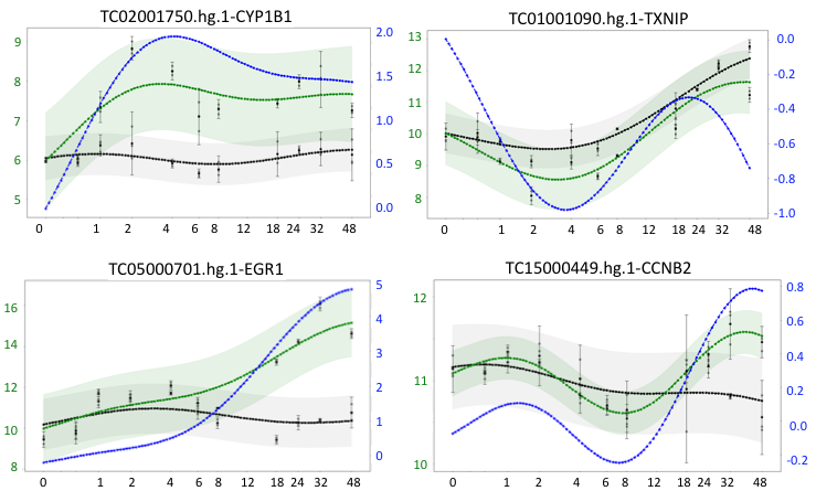
Figure 2: GP profiles for CYP1B1, TXNIP, EGR1, and CCNB2. The dots with whiskers are the input data. The black/green dotted line is the control/treated mean value (all log₂), sampled at 100 time points between 0 and 48 h. The blue dotted line is the (log₂) ratio (the difference between the green and black). The grey/green bands around the control/treated lines depict the 2 SD bands.

The GP (for Gaussian process) profiles are based on a distribution of continuous log₂ intensity profiles for control and treated samples for each transcript using Gaussian processes (described in [24]). Arrays of means and standard deviations (SD) for control and treated processes were generated by sampling the continuous distributions at 100 time points between 0 and 48 h chosen uniformly on a log scale. The ratio was then computed as the difference between the treated and control ($log_{2}(X/Y)=log_{2}(X)-log_{2}(Y)$). Maps associating transcripts to a number proportional to the space between the $1$ or $2$ SD bands around the control and treated means were defined. An approximation of the derivative of ratio time profile was computed as another view of the data. Figure 2 shows GP profiles for four transcripts with different features. The control 2 SD bands for CYP1B1, EGR1 and TXNIP are fairly narrow, and the control is basically flat for CYP1B1 and EGR1 while it is rising for TXNIP and has a small downward slope for CCNB2. CYP1B1 has substantial white space between the 2 SD bands during the middle times, while EGR1 has substantial white space between the 2 SD bands at the later times, indicating a significant change. TXNIP has no white space between the 2 SD bands, but does have white space between the 1 SD bands at 15 time points (computed from the control and treated SD profiles).

PCA and cluster analysis.

Principle Component Analysis (PCA) (based on ratio and on derivative GP profiles) was used for dimension reduction and to rank transcripts according to their contribution to overall variation. For the methamidophos data, three PCA components account for $95\%$ of the variation. We explored several standard clustering algorithms. In this study, we focused on $k$-means clustering with 128 clusters, as this clustering method seems to give the most useful information. Clusters were computed (for both ratio and derivative) using the PCA 3-dimensional representation of GP profiles. Clusters were annotated with GO process, GO function, and HUGO Gene Nomenclature Committee (HGNC) family terms using a heuristic method to compute likely classifications of a cluster from classifications of its elements. [24]

Ranking.

In addition to PCA ranking, autoencoder techniques were used to derive compressed representations of the GP profiles. Contrary to the usual criteria, the transcripts that are least accurately recovered are the potentially interesting ones, since they don’t behave like most transcripts, i.e. they are anomalies from the autoencoders perspective (see [24]). Generative Adversarial Network (GAN) techniques were used define two additional rankings: atypical/fake and typical/real. The GAN ranking algorithm is described in the next subsection.

2.3 Generative Adversarial Networks

Generative Adversarial Networks (GANs) [6] use a game-theoretic formulation to define the objective function of a machine learning problem. They involve two subnetworks, a generator and a discriminator that play against each other, so that ideally improvements in one network during training lead to corresponding improvements in the other until a Nash equilibrium is reached. Advantages of GANs are that they learn a generative model that approximates the full data distribution and they are less prone to overfitting than pure discriminative approaches due to the lack of a direct coupling between the generative model and the data. While there are other interesting generative applications (see e.g. [19]), we are primarily interested in obtaining a robust discriminator to distinguish time series anomalies from typical behavior.

Our training data set consists of $90\%$ (the other $10\%$ are used for validation) of the log-ratio time series (excluding the uninformative time $0$) for all genes estimated using Gaussian processes as explained in [24]. The data is locally normalized for each time point (to mean $0$ and unit variance) to abstract from the absolute magnitude. Our discriminator network with an input dimension of $100$ (size of the time series) consists of two layers, a 1D convolutional network (we use $20$ features, window sizes $21$, $41$, and $61$, stride $1$) with exponential linear unit (ELU) activation, followed by a dense layer with linear activation. Note that we deviate from the traditional convolutional architecture by not using a pooling layer for better stability of the training process. The generative network takes a $20$-dimensional normal distribution as an input, that is passed through a dense layer with ELU-activation resulting in a tensor of dimension $80\times 20$, $60\times 20$, or $40\times 20$, depending on the window sizes discussed above. Finally, we apply a transposed 1D convolutional layer to obtain a time series represented as a vector of dimension $100$. The GANs are specified using TensorFlow [1] and Edward [22], a framework for probabilistic programming that recently became part of TensorFlow Probability.[21] We use TensorFlow’s Adam optimizer with default settings with the standard GAN loss function. Each GAN is trained for $100000$ epochs with a batch size of $1000$ and achieved good convergence (based on the loss on the validation set) for all the window sizes. A second set of GANs with the same window sizes was trained on a globally normalized data set (over all time points and genes, thereby maintaining relative information about the magnitude of changes), which required a larger feature dimension of $50$ to achieve satisfactory convergence.

Finally, we applied the discriminators (for all window sizes and the two variations in terms of normalization) to the full set of log-ratio time series to obtain a score in the interval $[0,1]$ and a corresponding ranking of all genes, with values closer to $0$ denoting an anomaly (fake) and values closer to $1$ denoting a more typical (real) element of the overall time series distribution. The rankings based on globally normalized training data turned out to be more useful in our analysis, in that transcripts that are up/down regulated by 1 log₂ fold or have substantial 1 SD separation are more likely highly ranked (appear at the extremes of the ranking list) than transcripts that exhibit much smaller change and/or less separation of treated from control. Thus we used only the ranks based on globally normalized data in our analysis process.

2.4 Siamese Convolutional Networks

As discussed in more detail in [19] we decompose the problem of causality detection into two subproblems, each addressed by a type of Siamese neural network.[3] The first model is designed to detect and probabilistically quantify the existence of causality, while a second model is used to probabilistically determine its direction.

The undirected causality detector is a Siamese neural network, that is a neural network with two identical subnetworks that are each responsible for processing one of the arguments of the binary symmetric causality relation. Each argument is a time series (of size $w=80$ consistent with our synthetic data to be explained below). The replicated subnetwork is a 1D convolutional network (we use a window size $w^{\prime}=61$ and stride $1$) with bias and a rectified linear unit (ReLU) activation function yielding a tensor ($20\times 50$ dimensional). This is followed by an average pooling layer yielding a vector ($50$ dimensional), followed by a dense layer with the same output dimension and again with bias and relu-activation. Hence, the output of each subnetwork is a vector in feature space ($50$ dimensional). The two outputs are combined by a dot-product layer (which captures the symmetry of the problem as part of the architecture). As usual for Siamese networks, the symmetry is also exploited by weight-sharing between the two subnetworks. Finally, to obtain a probabilistic output, a sigmoid function is applied to a linear transformation of the scalar result from the dot-product, which can also be viewed as trivial dense layer with bias and sigmoid-activation. As a loss function we use binary cross-entropy and as an optimizer we use TensorFlow’s implementation of Adam (with default parameters).

The training and validation data set is based on a synthetic dynamic model, that we can only briefly summarize here and refer to [19] for more details. Using our Gaussian process as a template we generate positive and negative examples of causally related “synthetic” genes, or more precisely, corresponding time series that are biological plausible in the context of our experiment. There is a complexity parameter $m$ involved in the construction that we refer to as mixin-parameter. It allows us to vary the complexity of the synthetic model by limiting the number of genes that can participate in an interaction, which is modeled by a noisy linear superposition of time series sampled from our Gaussian processes model with a variable time lag. Employing curriculum training, we train the models with increasing complexity of the training data set. We use the mixin-parameter with settings $m=0,2,4$ to vary the complexity of the synthetic model. While we also explored higher parameters, we estimated that a target of $m=4$ should be sufficient for biologically plausible results. Each stage is trained for $1000$ epochs with a batch size of $20000$. Our synthetic data set contains $2000000$ pairs, from which we generate training and validation sets by random split of $90\%$ vs. $10\%$.

To detect the direction of an already established causality, we define a lag detector again a Siamese neural network, albeit a somewhat unconventional one detailed in [19], that after training estimates the lag in a normalized range $[-1,1]$.

As before, the replicated subnetwork is a 1D convolutional network with bias and a ReLU-activation function followed by a dense layer again with bias and ReLU-activation. Unlike in the causality detector there is no pooling layer involved. Hence, the output of each subnetwork is a tensor ($20\times 50$ dimensional). After flattening, the two outputs are combined by a subtraction layer (which captures the antisymmetry of the problem) yielding a vector (of dimension $1000$), The next layer is a dense layer without bias and tanh-activation reducing the dimension to $50$, and finally a linear dense layer without bias is used to obtain a scalar output. As a loss function we use mean square error and as an optimizer we again use TensorFlow’s implementation of Adam (with default parameters). The training and validation data set for the lag detector is generated in the same way as the (positive) synthetic pair set for the causality detector (again $1000000$ pairs), but we allow and track positive, negative, and zero time lags in the construction. Training and validation sets are then generated from this set of labeled pairs. For training we again use curriculum learning with the same parameters as for the causality detector.

We use these Siamese networks to synthesize two types of graphs. An undirected causal network is defined by nodes corresponding to all genes in a given subset and edges between pairs of genes for which the causality detector detects a dependency with at least the cutoff probability (another parameter in the graph synthesis process). A directed causal network is a refinement of an undirected causal network. Each edge is directed according to the prediction of the lag detector based on a positive threshold in the interval $(0,1]$ that was associated with a probability during validation. Each undirected edge becomes a directed edge if the lag prediction reaches at least the positive threshold and remains undirected otherwise.

As an example, the validated accuracy for the synthesized networks used in this paper using a synthetic model with mixin-parameter $m=4$) is $0.75$ for the existence of a causal relation and $0.72$ for its direction.

2.5 Time Warp Causal Inference

Time warp causal inference employs two primary algorithms for its operation: bootstrap resampling of the data and alignment of cause and effect events in time using the Needleman–Wunsch algorithm.[14] Comparison with N-th order, dynamic Bayesian networks indicates superior performance for time warp causal inference.

We begin by setting a threshold for significant fold change – a threshold of $2.0$ is common. A fold change over $2.0$ is considered high; below $1/2$ is considered low. For every transcript at every time point, there are two sets of concentration data: a treated set and a control set. The statistical t-test determines whether the means of the two sets are statistically different with a given confidence level. If the t-test indicates that they are different with satisfactory confidence, we can compute mean fold change (treated/control) to determine if the transcript is high or low at that point. Thus, the t-test can distinguish among three cases: high, low, and not statistically different. We need to distinguish among four cases: high, low, same (nominal), and too noisy to make a conclusion with high confidence. Data points that are too noisy may be treated as missing.

We are able to make the distinction among the four cases by using bootstrap resampling of the data. For a specific transcript at a given time point, assume each of the two data sets contains 3 concentration readings. With these two data sets, we can calculate 9 possible fold change ratios and then to calculate a mean fold change ratio for the data set. To bootstrap resample:

• Repeat 500 times

  • Sample with replacement the three readings in the treated set to make a new treated set

  • Sample with replacement the three readings in the control set to make a new control set

  • calculate the fold change ratio mean using the two, new data sets

• Sort the $500$ means to make a fold change distribution for this transcript at this time point

• Based on the desired confidence level (e.g. $85\%$), delete the extremes of the distribution

• Compare remaining distribution with fold change thresholds

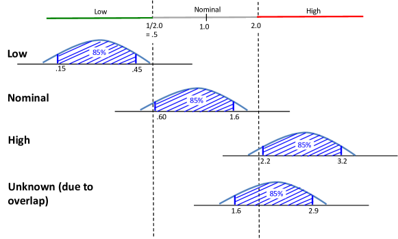
Figure 3: In the first distribution, the central $85\%$ of the distribution all lies below the low threshold of $0.5$, so the distribution is labeled low. In the second distribution, the central $85\%$ is between the low threshold and the high threshold of $2.0$, so this distribution is labeled nominal (treated and control are same). In the third distribution, the central $85\%$ all lies above the high threshold, so the distribution is labeled high. In the last distribution, the central $85\%$ overlaps both the nominal area and the high area, so this distribution is labeled unknown.

The Needleman-Wunsch alignment algorithm [14] is widely used for global, genetic sequence alignment. This algorithm uses an edit graph to align two genetic sequences, performing approximate matches to subsequences in arbitrarily different locations in each sequence by warping (adjusting) the space between the two sequences using insertions and deletions as appropriate. The algorithm uses dynamic programming that minimizes a cost function reflecting the cost of the insertions and deletions. To align cause and effect events with unknown, variable delays between cause and effect, time warp is needed (analogous to the way Needleman-Wunsch warps space in sequence alignment). To make our time warp edit graphs, each row and column of the edit graph is labeled with a value (high, nominal, or low) and the time of measurement. Unknown values are omitted. We then align the two event sequences using dynamic programming, preserving causality: effects events cannot precede cause events. A slightly higher cost is associated with aligning two events that are widely separated in time. Since causes can activate or inhibit effects, we initially match non-nominal events without regard to direction (high or low). Once the optimal alignment is identified, we produce both activate and inhibit alignment scores. For analysis purposes, we use the larger of the two scores exclusively. Figure 4 illustrates the algorithm. On the left, the subsequence “cg” is matched by the Needleman-Wunsch algorithm despite being offset in the two global sequences. On the right, the time warp causal inference algorithm matches both event pairs even though they have differing delays. N-order dynamic Bayesian networks are unable to find such matches.

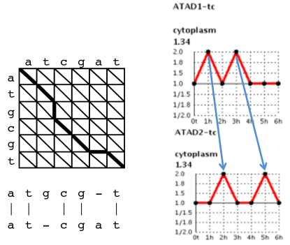
Figure 4: Timewarp illustration.

3 Results of data analysis

3.1 Global response features

Temporal distribution of response.

To get an idea of the shape of SK-N-AS cell response to methamidophos treatment we compute maps from transcripts to the first measured time when the log₂ ratio at that time is greater than $1$ (up by map) or less than $-1$ (down by map).

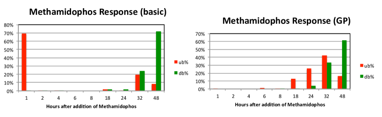
Figure 5: Up/Down By Charts showing the percent of transcripts up/down by (first crossing the 1 log₂ fold threshold) at each measured time point. (Left) computed using the basic time profiles. (Right) computed using the GP time profiles.

The results are summarized in Figure 5. The basic chart (left) shows a large spike of upregulation at 1h. Many of these transcripts show a peak at 1 h and little change at other times. Volcano plots (not shown) for the transcriptomics data suggest a possible experimental artifact at 1 h. This suggests the 1 h responders should be viewed with suspicion. This is smoothed away in the GP chart (right). Conversely, the basic chart shows little further action until 32 h while the GP chart shows substantial upregulation beginning at 18 h. This suggests that it is important to consider analysis based on both the basic time profiles and the GP time profiles, and to have multiple criteria for selection, to get the most out of the data.

Cell cycle.

We used the cyclin cell-cycle checkpoint markers CCNE2, CCNA2, CCNB2, and CCND1 to get a picture of the global cell cycle state of the cells after methamidophos exposure. Figure 6 shows the basic time profiles of these transcripts. We see a down regulation of CCNE2 from 18 h, indicating that the cells have has passed G1/S. There is a sustained upregulation of CCNA2 and CCNB2 starting at 32 h, indicating a G2 arrest at 32 h.

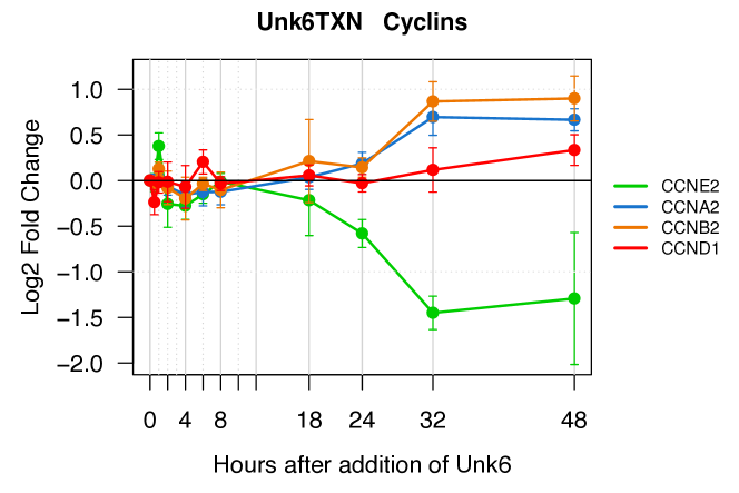
Figure 6: Cell-cycle state: Basic time profiles for Cyclins

Predicates.

We used the various ranking functions and significance filters to define predicates to select sets of transcripts to examine. Predicates upby t / dnby t are derived from the up/down chart maps. For $t$ one of the measured times, a transcript satisfies upby t (dnby t) if the log₂ ratio first passes $1$ ($-1$) at at time t. Thus for $t=18h$, upby t is the set of transcripts with log₂ ratio first exceeding 1 at 18 h. We defined a modest size (194) set of transcripts, named Top20X, to initially consider. Top20X consists of transcripts that are ranked in the top 20 of at least one of the ranking functions: PCA (ratio or derivative), any of 3 principal components positive or negative; GAN fake (atypical, anomalous) or real (typical), according to one of the three GAN models; or one of the autoencoders-based ranks. Furthermore transcripts in Top20X must have a (significant) log₂ fold change magnitude of at least 1 at some measured time, or have 1 SD separation of control and treated GP profiles for at least 15 (of 100) sampled times.

We note that of the transcripts upregulated by 1 h (recall the 1 hour spike in Figure 5) only 24 belong to Top20X. Of these, only TIPARP has sustained upregulation. It is classified GAN real. The rest are included in Top20X because of PCA ranking. This seems to confirm that although the 1 h data is suspect, perhaps it should not simply be dropped.

3.2 Candidate MoA Biological Processes

To identify cellular processes that are part of the SK-N-AS cell response to methamidophos, we examined GO process terms associated with responsive transcripts in several ways. PantherDB[13] was queried for over representation using several transcript sets (see Appendix 6.2 for details). For example, from the 545 transcripts upby 1 h, interferons were identified in an immune response group. From 155 transcripts upby 32 h, multiple process groups were found, including: metabolic processes, response to growth factors, circadian rhythm, chromatin related, and cell cycle. From 62 transcripts upby 48 h, heat shock and protein folding stood out. We also manually scanned GO process terms associated with clusters by our cluster analysis algorithm, and GO process terms associated with the Top20X transcripts by UniProt. Three process types stood out: unfolded protein response (UPR, including ER stress), cyclic adenosine monophosphate (cAMP) response, and calcium ion (Ca++) related processes. In addition, analysis of the data with the MIRU tool[27] found a cluster associated to cell-cell signaling, suggesting we look for cell-cell signaling indicators in our analysis (see Appendix 15 for details). Using the resulting process suggestions we investigated further.

Unfolded Protein Response (UPR).

Five transcripts were identified by Panther overexpression analysis of the upby 48 h transcripts as being annotated with UPR: HSPA1A, HSPA1B, HSPA5, HSPA6 and DNAJB1. The first four code for heat shock proteins. DNAJB1 stimulates the folding of unfolded proteins mediated by HSPA1A/B [7].

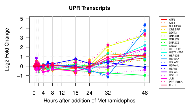
Figure 7: Time profiles of UPR transcripts.

From six clusters annotated with UPR related terms, nine transcripts were annotated with UPR related terms: BHLHE40, DNAJC2, HIST2H2BE, HSP90B1, HSPA4L, HSPA5, HSPH1, JUN, and XBP1. Five additional Top20X transcripts are annotated with UPR terms: CREBRF, DDIT3, GNG2, HSP90B1, HSPA4L, HSPA5, JUN, and PPP1R15A. Taken together we have seventeen transcripts associated to UPR based on our data analysis. Five are ranked in the top 20 GAN real (DDIT3, HIST2H2BE, HSPA5, JUN, PPP1R15A) and two are ranked in the top 20 GAN fake (CREBRF and GNG2). We also consulted the Reactome “Genes involved in Unfolded Protein Response” pathway and obtained 3 additional transcripts to consider: ATF3 DNAJC3 and HERPUD1. Finally, the paper [18] shows that the gene for ATF4 is upregulated at 12-24 h in response to three out of seven drugs commonly used as UPR inducers. In all, twenty one transcripts from Top20X were found to be related to UPR using GO annotations, pathway databases, and experimental results. Figure 7 shows the overlaid basic time profiles for these twenty one transcripts. For most of the transcripts, upregulation seems to start between 24-32 h, while HSPA1A and HSPA1B are downregulated 18-32 h and upregulated 32-48 h. Both GNG2 and HSPH1 are downregulated from 32-48 h.

Cyclic Adenosine Monophosphate (cAMP) response.

The cAMP-dependent pathway is a G protein-coupled receptor-triggered signaling cascade, activated by a number of toxins, with a role in many biological processes, including cell communication [2]. cAMP is produced by conversion of ATP by activated adenylate cyclase (also called adenylyl cyclase). The diterpene forskolin is used in experiments to study cAMP response, as it directly activates adenylate cyclase thus increasing the level of cAMP. Using time series transcriptomics data from HepG2/C3A cells treated with forskolin [23] we collected lists of transcripts up or downregulated early as a model of cAMP responsive genes.

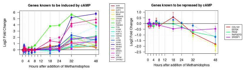
Figure 8: Time profiles of cAMP transcripts

Figure 8 shows plots of the time profiles of forskolin responsive transcripts that also show some response to methamidophos. Except for EGR1 (solid green) and the ZFPs (reddish) the up regulation appears to start around 24 h. The down regulation seems to begin around 18 h. This is consistent with a first phase of up regulation that produces something that activates adenylate cyclase. Of the twenty six upregulated transcripts suggested by the forskolin data, twelve are in the methamidophos Top20X: ARRDC3, BHLHE40, CPEB4, EGR1, FOS, GDF15, HSPA5, JUN, NR4A1, PER1, VGF, and ZFP36. Only five of these transcripts (FOS, HSPA5, JUN, PER1, and VGF) were in our set of cAMP annotated transcripts. On the other hand, ID4 and RELN were cAMP annotated and are not in the forskolin list. Of the five downregulated transcripts suggested by the forskolin data, two are in the methamidophos Top20X: COL1A1 and EEF2K. Both are cAMP annotated.

Calcium ion response.

Using UniProt GO process annotations we found twenty one Top20X transcripts annotated with calcium ion (Ca++) related terms.

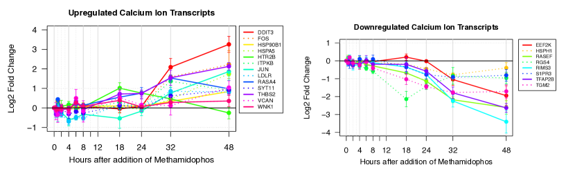
Figure 9: Profiles of calcium ion related transcripts.

Thirteen are upregulated (HTR2B up by 18h; DDIT3, FOS, ITPKB, LDLR, RASA4, THBS2, WNK1 down by 32 h; and HSP90B1, HSPA5, JUN, SYT11, VCAN up by 48 h) and eight are down regulated (RGS4, TGM2 down by 18 h; RASEF, RIMS3, S1PR3 down by 24 h; EEF2K, HSPH1, TFAP2B down by 32 h). Six of the upregulated and four of the down regulated Ca++ transcripts are ranked GAN real. Two of the upregulated Ca++ transcripts are ranked GAN fake. Figure 9 shows the expression profiles of these transcripts: upregulated on the left and downregulated on the right.

3.3 Conjectured acetylcholine build up

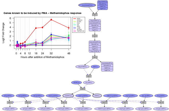
Figure 10: Response to acetylcholine buildup

The result of acetylcholine esterase inhibition in cultured cells is that acetylcholine builds up and binds and activates muscarinic and nicotinic acetylcholine receptors [4]. Since methamidophos is a cholinesterase inhibitor we looked for the consequences of a buildup of acetylcholine. Figure 10 shows a curated pathway leading from the binding of acetylcholine to the muscarinic receptor ChRm3 to upregulation of genes known to be upregulated by PMA, a diacylglycerol (DAG) mimic. This pathway corresponds to the production of DAG and IP3 via break down of PIP2 by activated PLC. We used the Pathway Logic Datum knowledge base[8], the derived PMA response network [9] and induction information from UniProt to identify the genes responding to PMA. The inset in Figure 10 shows the methamidophos response time profiles of these transcripts. Note that except for EGR1, these transcripts all are upregulated starting sometime after 24 h. EGR1 responds to many signals, what is possibly surprising is its delayed upregulation, as it is one of the immediate early genes. In addition to the DAG induced response, IP3 initiates intracellular calcium release, consistent with the Ca++ response noted above.

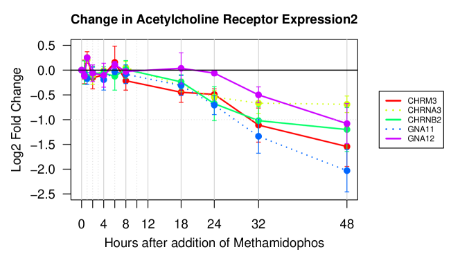
Figure 11: Down regulation of Acetylcholine receptors

The acetylcholine receptors CHRM3, CHRNA3, and CHRNB2, and GPCR binding partners components GNA11, GNA12 are downregulated starting around 18 h (see Figure 11 ). This could be additional evidence of acetylcholine build up, with the cell damping the response.

Overlapping roles.

There is non-trivial overlap between some pairs of process specific transcript lists. In particular, ARRDC3, EGR1, FOS, and JUNB belong to the PMA and cAMP lists; BHLHE40, HSPA5, and JUN belong to the UPR and cAMP lists; DDIT3, HSP90B1, HSPA5, HSPH1, and JUN belong to the UPR and Ca++ lists; and FOS, HSPA5, and JUN belong to the cAMP and Ca++ lists. The UPR and PMA lists do not overlap. HSPA5 and JUN belong to all lists except PMA and FOS belongs to all lists except UPR. Even though there are overlaps, each of the four process lists has many transcripts unique to that list.

3.4 Some distinguished transcripts

In addition to identifying processes potentially involved in SK-N-AS cell response to methamidophos, we are interested in identifying specific transcripts that might play significant roles. For this purpose we identified three different Top20X subsets: two based on GAN ranking combined with $k-$means clustering and one based on playing a role in multiple processes. In the following, HGNC transcript names are often followed by process annotations in parentheses.

GAN fake transcripts.

In six $k-$means clusters (three upregulated and three downregulated) at least half of the Top20X transcripts are GAN fake. This includes thirty-five of the forty seven Top20X GAN fake transcripts. The three upregulated clusters (27, 78, 127) are up by 32h. Cluster 27 contains nine GAN fake transcripts including CREBRF (UPR), DIAPH2 (actin filament organization), HDAC5 (chromatin organization), and RASA4 (Ca++). Cluster 78 contains five GAN fake transcripts, of which two, AHNAK and ITPKB, are Ca++ related. Cluster 127 contains four GAN fake transcripts including GJA1 (cell communication by electrical coupling) and IER2 (cell motility). Cluster 81, downregulated at 8 h, contains seven GAN fake transcripts including three associated to cholesterol biosynthetic process: DHCR7, HMGCS1, and NSDHL. Clusters 20 and 38 are downregulated at 48 h Cluster 20 contains four GAN fake transcripts including ACAT2 (cholesterol biosynthetic process) and TOE1 (Target of EGR1). Cluster 38 contains six GAN fake transcripts including GNG2 (protein folding, calcium modulating), ARHGAP28 (negative regulation of stress fiber assembly), and NEBL (actin filament binding).

GAN real transcripts.

The transcripts of eight $k$-means clusters (five upregulated, three downregulated) were all (with one exception) Top20 GAN real transcripts. Four of these clusters are singletons: CYP1B1, TIPARP, EGR1, and NEUROG2. TIPARP, a negative regulator of AHR, is the one transcript up at 1 h with sustained upregulation. CYP1B1 (toxin metabolic process) is up by 2 h and stays up. It is likely oxidizing the toxin. EGR1 (Early growth response protein 1, PMA, cAMP) a transcription factor, generally showing an early response to perturbations, is not up until 18 h. NEUROG2 (E-box binding transcription factor) is downregulated at 18h. The GAN real transcripts NR4A1, VGF, and ZFP36 form a triplet cluster upregulated at 18-32 h. This cluster is a subset of the cAMP responsive transcripts. The transcripts DDIT3 (UPR, Ca++), GDF15 (cAMP), PPP1R15A (UPR), and TFPI2 (extracellular matrix) form a cluster of size four upregulated at 32 h. TXNIP and RHOB form a doublet cluster downregulated early (2-4 h). One role of RHOB is actin filament bundle assembly. According to UniProt, TXNIP is known to be downregulated in response to oxidative stress. Txnip, the protein coded by TXNIP inhibits thioredoxin activity and the proteasomal degradation of Ddit4. TXNIP also stands out because it is in the top 20 real transcripts for one of the GAN models and in the top 20 fake transcripts in another of the GAN models. This dual ranking is rare. RGS4 (GAP, Ca++), HAND1 (transcription factor) and POPDC2 (cAMP-binding, regulation of membrane potential) form a triplet cluster downregulated at 18 h. POPDC2 is the exception, it is top 30 GAN real ranked. Finally, CACNG4 (membrane depolarization) and NCOA5 (glucose homeostasis and negative regulation of insulin receptor signaling) form a cluster of 2 downregulated at 18 h. The remaining GAN real transcripts appear in clusters where most elements are not GAN ranked. For example cluster 66 has 5 elements, all in the UPR process list, only two (HIST2H2BE and JUN) are top 20 GAN real.

Multirole transcripts.

Thirteen transcripts were selected from the Top20X because they were annotated by multiple specific GO process terms that stood out in a scan of the UniProt GO annotations or in multiple Panther overrepresentation groups.

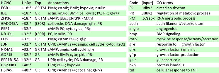
Figure 12: Multirole transcripts. PMA, UPR, cAMP, and Ca++ refer to the process groups discussed in section 3.2. UPR includes unfolded protein response; ER stress, protein folding Ca++ includes calcium ion release, sequestering and transport. The P in PC,PR,PM indicate annotations derived from Panther analysis.

The table in Figure 12 summarizes these transcripts with their annotations. Except for PER1 and HSP901B1 all are top 30 GAN real ranked and of the latter all but GADD45A and NR1D1 are top 20 GAN real ranked. Three of the four processes already identified are well represented: UPR 4, Ca++ 6, and cAMP 8. Five of the transcripts are annotated with cell cycle. Three are annotated with BMP signaling, three with cytokine related processes, three with angiogenesis and three with circadian rhythm (PC). Six are annotated with growth factor related terms and seven are annotated with regulation of metabolic processes.

3.5 Inferred causal relations

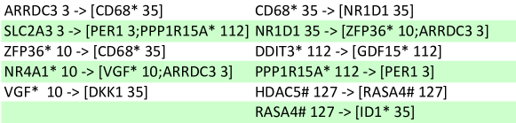
Figure 13: Sample Edges from the Siamese Network

Figure 13 shows a sample of the top 200 causal relations proposed by the Siamese Convolutional algorithm restricted to transcripts in Top20X. * indicates top 20 GAN real ranking and # indicates top 20 GAN fake ranking. The numbers are cluster identifiers. We see that edges are often within a cluster, and clusters 3, 10, 35, 112, 127 form a connected component.

The algorithm is more confident about the existence of an edge than about the direction. Thus the fact that we see cycles such as NR1D1-[ZFP36,ARRDC3]-CD68-NR1D1 is not totally surprising. What it says is that more information is needed to refine the relations. The causal relation between DDIT3 (aka CHOP) and GDF15 in the context of ER stress is supported by work reported in Li et al [11]. We have not yet found evidence supporting or disagreeing with the other hypothesized relations.

The following is a sample of the top 1600 causal relations proposed by the Time warp causal inference algorithm restricted to transcripts in Top20X.

ARRDC3 BHLHE40 CPEB4# CREBRF# DDIT3* FAM72D FOS* GADD45A GDF15*
H1F0 HDAC5# ID4# IER2# ITPKB# NR4A1* PER1 PPP1R15A* SERPINE1
SLC2A3 TFPI2* THBS2 ZNF550
-b>  [HIST2H2BE*, HSPA5*, RELN]

Gene set enrichment analysis (GSEA) analysis against the hallmark gene sets in the Broad Molecular Signatures Database showed overlaps of BHLHE40 FOS DDIT3 SLC2A3 SERPINE1 HSPA5 PPP1R15A with the Hallmark-Hypoxia data set. The data set contains 200 genes upregulated in response to low oxygen levels (hypoxia). BHLHE40 FOS DDIT3 SLC2A3 SERPINE1 HSPA5 THBS2 NR4A1 showed overlaps with the Winter-Hypoxia-Metagene data set. The data set contains 242 genes regulated by hypoxia, based on literature searches. In addition, RELN was shown to be regulated by Hif1 alpha and Hif2 alpha in [16]. Hypoxia has been known for a long time to cause ER stress [28] and HIST2H2BE, HSPA5 are among the transcripts identified above as part of the UPR response. The ENCODE Transcription Factor Binding Site Profiles dataset shows that the promoters for HIST2HBE, HSPA5 and RELN all have binding sites for BHLHE40 and that HIST2HBE and HSPA5 also have binding sites for FOS.

4 Materials and methods

4.1 Data Generation

Cell Culture and Exposure.

SK-N-AS cells (ATCC^® CRL-2137) were seeded at $5\times 10^{5}$ cells per well in 12-well plates (Thermo Scientific^TM BioLite 12-556-005) in Dulbecco’s modified Eagle’s medium (DMEM, ATCC^® 30-2002). The medium was supplemented with $10\%$ fetal bovine serum (FBS, ATCC^® 30-2020), 50 units/mL of penicillin, and 50 µg/mL of streptomycin (Gibco^TM 15-070-063), and $1\%$ MEM non-essential amino acids solution (Gibco^TM 11-140-050). Cells were incubated at $37^{\circ}$C and $5\%$ CO₂ for 0.5-48 h with or without methamidophos 2 mg/mL (Sigma-Aldrich 33395 and LGC Standards DRE-C14980000). Growth medium was removed and cells were mixed with RNAprotect Cell Reagent (Qiagen 76526) and frozen at $-80^{\circ}$C until analysis.

HepG2/C3A cells (ATCC^® CRL-10741) were seeded at $1\times 10^{5}$ cells per well in 12-well plates (Thermo Scientific^TM BioLite 12-556-005) in Eagle’s minimum essential medium (EMEM, ATCC^® 30-2003). The medium was supplemented with $10\%$ fetal bovine serum (FBS, ATCC^® 30-2020), 50 units/mL of penicillin, and 50 µg/mL of streptomycin (Gibco^TM 15-070-063). Cells were incubated at $37^{\circ}$C and $5\%$ CO₂ for 1-48 h with or without forskolin 25 µM (R&D Systems 1099/10). Growth medium was removed and cells were mixed with RNAprotect Cell Reagent (Qiagen 76526) and frozen at $-80^{\circ}$C until analysis.

RNA Preparation and Microarray Processing.

Total RNA was extracted from control and treated triplicate exposures using Qiagen’s RNeasy Plus Micro kit following the manufacturer’s protocol with an additional on-column DNase1 treatment. RNA concentration (Nanodrop ND-1000, ThermoScientific) and quality (Agilent’s 2100 Bioanalyzer with RNA Nano kit) were determined prior to whole transcriptome expression analysis using the GeneChip^TM WT PLUS Reagent Kit and GeneChip^TM Human Transcriptome Array 2.0 microarrays (ThermoFisher Scientific). According to manufacturer’s protocols, 100 ng total RNA was converted to ss-cDNA and 5.5 ${\mu}$g ss-cDNA was fragmented and labeled. Hybridization and scanning were performed by the Stanford University PAN facility. Data files were processed to determine transcript level average signal intensities using Affymetrix Expression Console (build 1.4.1.46) and Transcriptome Analysis Console 3.0 software and annotation file hta-2-0.na34.hg19.transcript.

5 Discussion, Related and Future Work

Discussion.

We confirmed that our suite of analysis algorithms worked when applied to data from a new cell line treated with a different type of challenge without need to adjust parameters. We used our novel ranking algorithms combined with significance change filters to select a set of transcripts as a starting point. Our data analysis then found four processes as candidate elements of the broader MoA of methamidophos: UPR, cAMP response, calcium ion related processes, and cell-cell signaling. For each process we identified responding transcripts likely to participate in that process using a combination of GO process annotations, data from other experiments and pathway databases. We also curated a model of acetylcholine buildup as a consequence of the inhibition of acetylcholinesterase (ACHE). The resulting model suggested three downstream effects: increase in DAG (PMA response), increase in IP3, and active G-protein-coupled receptor (GPCR). Increase in IP3 induces release of calcium ion consistent with the identified calcium ion related response. The cAMP response could be connected to the acetylcholine signal through the G protein binding partners of ChRm3 or the calcium ion release.[25] G2 arrest (identified by cyclin profiles) is a pause in the cell life cycle due to detected problems, such as DNA damage. Nine of the Top20X transcripts are annotated with DNA damage related terms. The strong UPR response suggests another reason for a G2 arrest. We identified a number of transcripts that are potentially key elements of the MoA using the GAN fake/real ranking and multirole annotations. Some participate in already identified processes. The results suggest investigating cell cycle and metabolic (especially cholesterol) processes in more detail. Finally, results from two different causal inference algorithms suggested new connections as well as finding some known connections. Although the biological results are maybe not surprising, we were encouraged by the fact that the pure data analysis pulled out transcripts that when further examined in the light of known biology lead to reasonable hypotheses.

Related work.

Existing approaches to arrive at MoA candidates from omics data include enrichment and network perturbation analysis methods to infer causal networks. Enrichment analysis such as Ingenuity^® Pathway Analysis (Qiagen)  [10] and PANTHER [13] rely on extensive curated information to identify candidate pathways and processes. They provide important information but are limited by what interactions and pathways researcher have focused on and may miss important aspects. The detecting mechanism of action by network dysregulation (DeMAND) algorithm [26] infers the MoA of small molecule compounds by looking for dysregulation of their molecular interactions following compound perturbation. It requires an interaction network as input as well as gene expression profiles of control and treated samples. Multiple timepoints can be used, but they are treated independently. Protein target inference by network analysis (ProTINA) [15] also uses network perturbation analysis method for inferring protein targets of compounds from gene transcriptional profiles. The input network models are specific to the experimental context and represent transcription factor to gene interactions. Dynamic models of gene expression are derived from these networks enabling ProTINA to leverage the information in timeseries gene expression profiles. Our analysis of the response to methamidophos used several available knowledge bases to classify groups of responsive transcripts, but did not require a prior interaction/gene regulation network.

In [17] the objective is to identify a set of core differentially expressed transcriptional regulators in the TLR-stimulated macrophage and the clusters of co-expressed genes that they may regulate. The methods used include clustering of expression time profiles; GO annotations of the gene clusters; time-lagged correlation; and promoter sequence scanning for transcription factor (TF) binding sites recognized by a differentially expressed TF. This approach to analysis of timeseries transcriptomics data is closer in spirit to our work and suggests our analysis might benefit from looking at promoter sequences to refine the inferred causal relations.

The analysis was able to recover many known regulators, and also identified a potential transcriptional regulator not previously known to play a direct role in TLR-stimulated macrophage activation, TGIF1. The review [29] discusses additional work by the ISB group using similar techniques to infer transcriptional relations from time series data measured over a variety of conditions.

Li et. al. [12] treated SK-N-SH human neuroblastoma cells with three organophosphates including methamidophos with high and low doses for 24h and analyzed the resulting transcriptomics data. The doses for methamidophos were roughly 10 and 200 times the concentration used in the present study. The objective was a comparative study and since they found little common responsed they combined the data for the three experiments for fold change analysis. Thus we can not make a meaningful comparison with our results based on the results reported in the paper.

Future directions.

Our analysis revealed potentially interesting downstream effects of methamidophos and also suggests a number of interesting future directions. One is developing methods to better understand which of the multiple predicted roles different transcripts are playing and when. Another future direction is understanding the meaning of edges in graphs synthesized using algorithms with different assumptions to understand in what sense are they “causal”. The two algorithms used in the present study to infer causal relations from timeseries data give qualitatively different, complementary views of the potential causal network hidden in the data. The timewarp algorithm produces short chains (in theMethamidophos case, length 1) and clustered relations– pairs of groups of compounds where there is an edge from every element of one group, to every element of the other group as illustrated above. In contrast, the Siamese Twin algorithm produces longer chains of causality edges with more diversity of connections (a sparser graph). One reason is likely the discrete treatment of time and expression levels used by the timewarp algorithm. As both views seem to provide useful information, more work is needed to understand the precise biological interpretation of the inferred networks. A first step might be taking into account available promoter binding information, but much more work is needed here. For example, can we extract interpretable features that the machine learning algorithms find? Will that help with understanding the anomalies and the derived “causal” relations?

6 Appendix

6.1 Predicate details

We define a number of predicates used to select subsets of transcripts and compare them. Roughly they concern qualitative measures of significance (signal vs. noise), measures of change, and ranking functions indicating the presence of distinctive/discriminating features.

6.1.1 Measures of significance and change

Measures of significance.

The predicate $\mathit{sep}(d,n)$ holds for a transcript if there is white space (non-overlap/separation) between $d$ standard deviation bands around treated and control GP time profiles for at least $n$ (of $100$) time points. Thus $\mathit{sep}(1,15)$ holds for a transcript if the 1 standard deviation bands around the GP treated and control time profiles do not overlap for at least $15$ time points. A measured time is called o-significant if the treated and control measurements define non-overlapping intervals.

Measures of change.

In the following we give the predicate name (a short name usable to label rows and columns) and the definition for measure of change predicates.

• 2sd : $\mathit{sep}(2,1)$

• 1sd : $\mathit{sep}(1,1)$

• 1sd33 : $\mathit{sep}(1,33)$

• 1sd15 : $\mathit{sep}(1,15)$

• 67sd33 : $\mathit{sep}(.67,33)$

• udby1 : change of at least 1 log2 fold (at some o-significant measured time)

• udby2 : change of at least 2 log2 fold (at some o-significant measured time)

• nsig6 : at least 6 o-significant measured time points

• good : udby1 or 2sd

6.1.2 Ranking functions

We defined three groups of functions to rank transcripts according to some measure of possible importance. The functions are represented as lists of elements in order of decreasing rank.

PCA.

There are 6 PCA ranking functions two for each of the top 3 PCA components (one positive and one negative). The rank corresponds to the importance/weight of transcript in the given PCA component.

Anom.

This ranks transcripts according to quality of the GP profile reconstructed from the autoencoders representation. The worse the reconstruction quality the higher the rank, viewing the profile as representing anomalous behavior.[24]

GAN.

Generative Adversarial Network models rank transcripts according to how confident the trained discriminator is that the GP profile represents a transcript. High fake ranking cooresponds to low confidence that a profile comes from a transcript (i.e. high confidence it is not), and high real ranking corresponds to high confidence that the profile represents a transcript. We use three models parameterized by the feature window size (Section LABEL:nn-gan).

6.1.3 Discriminators.

In the following we give the predicate name (a short name usable to label rows and columns) and the definition for discriminator predicates.

• t20PCA : ranked in the top 20 in some PCA component

• t20an : ranked in the top 20 by some anomaly measure

• t20gf : ranked top 20 fake by some GAN discriminator

• t20gr : ranked top 20 real by some GAN discriminator

• t20 : top20PCA or top20Anom or top20gan-fake or top20gan-real

• t20x : t20 and (1sd15 or udby1) also known as Top20X

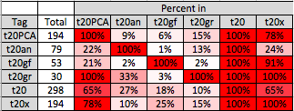
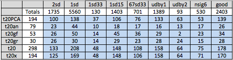
Figure 14: Comparing transcript sets

In the tables of figure 14 the size of the different sets and their intersections are shown. In the top two tables the entries $n$ (other than the total column) is read $n\%$ of elements in the set given by the row label belong to the set given by the column label. In the bottom table the entries simply represent the size of the intersection.

6.2 Panther over representation analysis results

We used the gene-list analysis service provided by the PantherDB website (www.pantherdb.org). HGNC gene ids were uploaded from files. We selected Statistical overrepresentation test, using the default settings and Homo Sapiens organism. The results are presented as a tree of GO-slim process terms. Each node is associated with information includeing the elements of the uploaded gene-list that are annotated with the nodes process term and the fold enrichment. Results were limited to those with FDR P-value $<0.05$.

Nine different transcript sets defined using predicates of section 6.1 were analyzed. The following summarizes the results: the predicate, the size of the set (in parens), number of GOSlim leaves. Each header is followed by a list of process terms, each with the number of associated transcripts and the fold enrichment.

• Top20X (194) no significant results

• udby1 (1389) no significant results

• udby2 (93)

  • circadian rhythm [3, 36]

  • regulation of metabolic process [18, 3]

• 67sd33 (701)

  • rRNA processing [15, 4.26]

    • RNA metabolic process [37, 2.3]

      • aromatic/nucleobase-containing compound metabolic process [52, 2.3]

• up log₂ fold by 1 hr (545)

  • lymphocyte proliferation (Interferons) [7, 7]

  • detection of chemical stimulus involved in sensory perception (olfactory receptors) [24, 4.5]

  • localization [23, .48]

  • cellular metabolic process [12, .31]

• up log₂ fold by 32h (155) leaves grouped in informal categories

  • Metabolic (Aldo-keto reductases, R:bile acid synthesis)

    • prostaglandin metabolic process [3, 57]

    • secondary metabolic process [3, 28]

    • hormone metabolic process [4, 23]

  • Growth factor response (negative)

    • response to fibroblast growth factor [3, 57]

    • cellular response to growth factor stimulus [3, 15]

  • negative regulation of MAP kinase activity [5, 50]

  • (regulation of) circadian rhythm [3+5 49,35]

  • Chromatin related (6 terms)

    • chromatin assembly or disassembly [3, 30]

    • negative regulation of chromatin silencing [3, 30]

    • negative regulation of DNA recombination [3, 21]

    • nucleosome organization [3, 20]

    • chromosome condensation [3, 18]

    • chromatin silencing [4, 14]

  • cellular response to peptide hormone stimulus [3, 30]

  • response to radiation [3, 17]

  • cell development [6, 7]

  • regulation of cell cycle [9, 7]

  • localization [3, .21]

• dn log₂ fold by 32h (146)

  • mRNA polyadenylation [4, 21]

  • DNA metabolic process [12, 5]

• up log₂ fold by 48h (62)

  • Heat shock related (3 terms total 6 47-92)

    • cellular response to unfolded protein [3, 92]

    • cellular response to heat [4, 47]

    • chaperone-mediated protein folding [6, 55]

  • nucleosome assembly [5, 47] (Histones)

• dn log₂ fold by 48h (433)

  • transcription, DNA-templated [47, 2] (17 ZNFs)

Notice that localization is underrepresented in the 67sd33 and upby 32 h transcript sets.

6.3 Cell-cell signaling.

Following up on the suggestion of cell-cell signaling response from the Miru analysis, we found that three $k$-means clusters have cell-cell signaling annotation. Interestingly, these clusters also have the G protein-coupled receptor signaling pathway annotation. Members of these clusters all have an upregulation peak at 1 h. No members of theses clusters with cell cell signaling annotation are in Top20X, so we selected transcripts that are either up or downregulated by 1 log₂ fold at some time, or pass the 2 standard deviation separation test. We call these ‘good’.

• Cluster 55 has 7 good transcripts with cell-cell signaling annotation: CCR5 FGF16 FGF6 GJA3 IAPP IFNA2 IL17A

• Cluster 116 has 2 good transcripts with cell-cell signaling annotation: CCL13 IFNA7

• Cluster 124 has 1 good transcript with cell-cell signaling annotation: CCL7

Figure 15 shows the time profiles of these transcripts. We see the 1 h spike followed by rather unsettled but low level response.

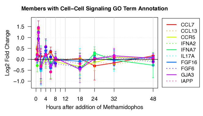
Figure 15: Basic time profiles of cell-cell signaling annotated transcripts

FGF6, FGF16 are growth factors and GJA3 is a gap junction protein. According to Wikipedia, IAPP (aka DAP, Amylin, or islet amyloid polypeptide), is a 37-residue peptide hormone that selectively regulates glucose metabolism. The rest are immune response proteins.

We checked the Top20X transcripts and found that only one, GDF15, is annotated with cell-cell signaling. The basic time profile of GDF15 has .7 log₂ ratio at 1 h, but then no measurable response until 32 h (where its has a 2 log₂ ratio). Clearly, having data measuring what is secreted would help to determine if cell-cell signaling is a real response and how it fits with other processes.

6.4 Distinguished transcripts

GAN fake cluster details.

In the following we list each GAN fake cluster, its GAN fake members and key associated GO terms, if any. I the first item “kmr27” identifies $k$-means ratio cluster 27. “(+32:*)” says the cluster is upregulated (+) at 32h and stays up (*) (to the end of the measured times). “9 fake of 10 Top20X of 24 total” says the cluster has 24 members, 10 of which are Top20X, and 9 of these are ranked GAN fake.

• kmr27 (+32:*) 9 fake of 10 Top20X of 24 total

  • CREBRF - negative regulation of endoplasmic reticulum unfolded protein response

  • DIAPH2 - actin filament organization

  • ERMP1 - metal ion binding

  • HDAC5 - chromatin organization; response to LPS and to insulin

  • IDS - glycosaminoglycan catabolic process

  • LACTB - regulation of lipid metabolic process

  • RASA4 - Ca++; negative regulation of Ras protein signal transduction

  • SPRY4 - negative regulation of Ras protein signal transduction

  • ZNF550

• kmr78 (+32:*) 5 fake of 10 Top20X of 39 total

  • AHNAK - regulation of voltage-gated calcium channel activity

  • ARMCX1

  • ITPKB - Ca++; inositol phosphate biosynthetic process

  • SMAD9 - cellular response to BMP stimulus

  • TBX20 - negative regulation of SMAD protein complex assembly; muscle contraction

• kmr127 (+32:*) 4 fake of 6 Top20X of 28 total

  • GJA1 - cell communication by electrical coupling; positive regulation of I-kappaB kinase/NF-kappaB signaling

  • ID4 - transcription factor; circadian rhythm

  • IER2 - cell motility

  • MIDN - negative regulation of glucokinase activity;

• kmr81 (min@8h) 7 fake of 7 Top20X of 36 total

  • ARFGAP2 - endoplasmic reticulum to Golgi vesicle-mediated transport; GTPase activator activity

  • DHCR7 - cholesterol biosynthetic process; 7-dehydrocholesterol reductase activity

  • HMGCS1 - cellular response to cholesterol; cholesterol biosynthetic process

  • METTL12 - protein methylation

  • NSDHL - cholesterol biosynthetic process

  • TSPYL4

  • UBXN8 - ubiquitin-dependent ERAD pathway (targeting ER-resident proteins for degradation)

• kmr20 (-48:*) 4 fake of 4 Top20X of 58 total

  • ACAT2 - cholesterol esterification; cholesterol O-acyltransferase activity; cholesterol biosynthetic process

  • LANCL2 - negative regulation of transcription

  • PHF23 - positive regulation of protein ubiquitination

  • TOE1 - (Target of EGR1) RNA phosphodiester bond hydrolysis,

• kmr38 (-48:*) 6 fake of 10 Top20X of 46 total

  • ARHGAP28 - negative regulation of stress fiber assembly

  • FNTB - protein farnesylation;

  • GNG2 - G protein-coupled receptor signaling pathway; adenylate cyclase-activating

  • IGFBP4 - regulation of glucose metabolic process

  • NEBL - actin filament binding

  • PIGA - phosphatidylinositol N-acetylglucosaminyltransferase

Note that Cluster 81 has several cholesteral related transcripts. Also (not shown) the graphs generated by several algorithms predict that HMGCS1 is well-connected. It is interesting to consider if some Cholestorol pathway has a specific role or it is a generic response.

GAN real clusters.

In the following we list each GAN real cluster, its GAN real members and key associated GO terms, if any. The notation is the same as for GAN fake clusters.

• kmr83 (+1:*) 1 real of 1 Top20X of 1 total

  • TIPARP - Acts as a negative regulator of AHR which inhibits PER1 expression cellular response to organic cyclic compound

• kmr44 (+2:*) 1 real of 1 Top20X of 1 total

  • CYP1B1 - toxin metabolic process

• kmr10 (+18-32:*), 3 real of 3 Top20X of 3 total

  • NR4A1 - cAMP; negative regulation of cell cycle

  • VGF - cAMP; cellular protein metabolic process; glucose homeostasis; insulin secretion;

  • ZFP36 - cAMP; mRNA catabolic process; negative regulation of polynucleotide adenylyltransferase activity;

• kmr42 (+18:*) 1 real of 1 Top20X of 1 total

  • EGR1 - transcription factor; protein refolding; negative regulation of cell proliferation; regulation of protein ubiquitination

• kmr112 (+32:*) 4 real of 4 Top20X of 4 total

  • DDIT3 - UPR; Ca++; cell cycle arrest; cellular response to DNA damage stimulus

  • GDF15 - cAMP; BMP signaling pathway; cell-cell signaling;

  • PPP1R15A - UPR; cell cycle arrest; cellular response to DNA damage stimulus; negative regulation of protein dephosphorylation

  • TFPI2 - extracellular matrix structural constituent; serine-type endopeptidase inhibitor activity

• kmr63 (-2,4:*) 2 real of 2 Top20X of 2 total

  • RHOB - actin filament bundle assembly; positive regulation of angiogenesis; endosome to lysosome transport

  • TXNIP - Ca++; cell cycle; negative regulation of cell division; response to hydrogen peroxide/glucose

• kmr85 (-18:*) 1 real of 1 Top20X of 1 total

  • NEUROG2 - E-box binding transcription factor

• kmr71 (-18:*) 3 real of 3 Top20X of 3 total

  • HAND1 - transcription factor

  • RGS4 - negative regulation of G-protein coupled receptor protein signaling pathway; G-protein alpha-subunit binding calmodulin binding;

  • POPDC2 - cAMP-binding, regulation of membrane potential

• kmr87 (-18,24:*) 2 real of 2 Top20X of 2 total

  • CACNG4 - membrane depolarization; neurotransmitter receptor internalization; positive regulation of AMPA receptor activity

  • NCOA5 - glucose homeostasis; negative regulation of insulin receptor signaling pathway

References

- [1] Abadi, M., et. al.: Tensorflow: A system for large-scale machine learning. In: Proceedings of the 12th USENIX Conference on Operating Systems Design and Implementation. pp. 265–283. OSDI’16, USENIX Association (2016)
- [2] Alberts, B., et. al.: Essential cell biology (2nd ed.). Garland Science, New York (2004)
- [3] Bromley, J., Guyon, I., LeCun, Y., Säckinger, E., Shah, R.: Signature verification using a ”siamese” time delay neural network. In: Cowan, J.D., Tesauro, G., Alspector, J. (eds.) Advances in Neural Information Processing Systems 6, pp. 737–744. Morgan-Kaufmann (1994)
- [4] Colovi, M.B., Krsti, D.Z., Lazarevi-Pati, T.D., Bondi, A.M., Vasi, V.M.: Acetylcholinesterase inhibitors: pharmacology and toxicology. Curr Neuropharmacol 11(3), 315–335 (May 2013)
- [5] Consortium, U.: Uniprot: a wroldwide hub of protein knowledge. Nucleic Acids Research 47, D506–D515 (2019)
- [6] Goodfellow, I.J., et. al.: Generative adversarial nets. In: Proceedings of the 27th International Conference on Neural Information Processing Systems - Volume 2. pp. 2672–2680. NIPS’14, MIT Press (2014)
- [7] J.N., R., E., G.J.: Binding of human nucleotide exchange factors to heat shock protein 70 (hsp70) generates functionally distinct complexes in vitro. Journal of Biological Chemistry 289(3), 1402–14 (2014)
- [8] Knapp, M.: Pla datums (2019), pl.csl.sri.com/datumkb.html, last accessed 2019 March 14
- [9] Knapp, M.: STM8: A pathway logic model of intracellular signal transduction (2019), pl.csl.sri.com/online.html, last accessed 2019 March 14
- [10] Kramer, A., Green, J., Pollard, J., Tugendreich, S.: Causal analysis approaches in ingenuity pathway analysis. Bioinformatics 30(4), 523–530 (2014)
- [11] Li, D., Zhang, H., Zhong, Y.: Hepatic gdf15 is regulated by chop of the unfolded protein response and alleviates nafld progression in obese mice. Biochemical and Biophysical Research Communications 498, 388–394 (2018)
- [12] Li, T., Zhao, H., Hung, G.C., Han, J., Tsai, S., Li, B., Zhang, J., Puri, R.K., Lo, S.C.: Differentially expressed genes and pathways induced by organophosphates in human neuroblastoma cells. Experimental Biology and Medicine 237, 1413–1423 (2012)
- [13] Mi, H., et. al.: Panther version 11: expanded annotation data from gene ontology and reactome pathways, and data analysis tool enhancements. Nucleic Acids Research 45(D1), D183–D189 (2017)
- [14] Needleman, S.B., Wunsch, C.D.: A general method applicable to the search for similarities in the amino acid sequence of two proteins. Journal of Molecular Biology 48(3), 443–453 (1970)
- [15] Noh, H., Shoemaker, J.E., Gunawan, R.: Network perturbation analysis of gene transcriptional profiles reveals protein targets and mechanism of action of drugs and influenza a viral infection. Nucleic Acids Research 46(6), e34 (2018)
- [16] Ralph, G.S., et. al.: Identification of potential stroke targets by lentiviral vector mediated overexpression of HIF-1 alpha and HIF-2 alpha in a primary neuronal model of hypoxia. J. Cerebral Blood Flow Metabolism 24(2), 245–58 (2004)
- [17] Ramsey, S.A., et. al.: Uncovering a macrophage transcriptional program by integrating evidence from motif scanning and expression dynamics. PLOS Computational Biology 4(3), 1–25 (2008), https://doi.org/10.1371/journal.pcbi.1000021
- [18] Shinjo, S., Mizotani, Y., Tashiro, E., Imoto, M.: Comparative analysis of the expression patterns of upr-target genes caused by upr-inducing compounds. Bioscience, Biotechnology, and Biochemistry 77(4), 729–35 (2013)
- [19] Stehr, M.O., Avar, P., Korte, A.R., Parvin, L., Sahab, Z.J., Bunin, D.I., Knapp, M., Nishita, D., Poggio, A., Talcott, C.L., Davis, B.M., Morton, C.A., Sevinsky, C.J., Zavodszky, M.I., Vertes, A.: Learning causality: Synthesis of large-scale causal networks from high-dimensional time series data. CoRR abs/1905.02291 (2019), http://arxiv.org/abs/1905.02291
- [20] Talcott, C.: Summary of top20x transcripts in response to methamidophos (2019), http://www.csl.sri.com/users/clt/XYZ/sumG-top20ud1s1x-u6.xlsx
- [21] TensorFlow Probability: A library for probabilistic reasoning and statistical analysis: https://www.tensorflow.org/probability
- [22] Tran, D., Hoffman, M.D., Saurous, R.A., Brevdo, E., Murphy, K., Blei, D.M.: Deep probabilistic programming. In: International Conference on Learning Representations (2017)
- [23] Vertes, A., et. al.: Integrative systems biology approach to identify mechanisms of action (2016), abstract and poster US HUPO 2016 Conference
- [24] Vertes, A., et. al.: Inferring mechanism of action of an unknown compound from time series omics data. In: Ceska, M., Safranek, D. (eds.) Computational Methods in Systems Biology. LNBI, vol. 11095. Springer (2018)
- [25] Willoughby, D., Cooper, D.M.F.: Organization and Ca++ regulation of adenylyl cyclases in camp microdomains. Physiolical Reviews 87(3), 965––1010 (2007)
- [26] Woo, J.H., et. al.: Elucidating compound mechanism of action by network perturbation analysis. Cell 162(2), 441–451 (2015)
- [27] Wright, D., Angus, T., Enright, A., Freeman, T.: Visualisation of biopax networks using biolayout express3d. F1000Research (2014)
- [28] Xu, C., Bailly-Maitre, B., Reed, J.C.: Endoplasmic reticulum stress: cell life and death decisions. J. Clinical Investigation 115(10), 2656–64 (2005)
- [29] Zak, D.E., Aderem, A.: Systems biology of innate immunity. Immunology Review. 227(1), 264–282 (2009)