AutoGAN: Neural Architecture Search for Generative Adversarial Networks

Abstract

Neural architecture search (NAS) has witnessed prevailing success in image classification and (very recently) segmentation tasks. In this paper, we present the first preliminary study on introducing the NAS algorithm to generative adversarial networks (GANs), dubbed AutoGAN. The marriage of NAS and GANs faces its unique challenges. We define the search space for the generator architectural variations and use an RNN controller to guide the search, with parameter sharing and dynamic-resetting to accelerate the process. Inception score is adopted as the reward, and a multi-level search strategy is introduced to perform NAS in a progressive way. Experiments validate the effectiveness of AutoGAN on the task of unconditional image generation. Specifically, our discovered architectures achieve highly competitive performance compared to current state-of-the-art hand-crafted GANs, e.g., setting new state-of-the-art FID scores of 12.42 on CIFAR-10, and 31.01 on STL-10, respectively. We also conclude with a discussion of the current limitations and future potential of AutoGAN. The code is avaliable at https://github.com/TAMU-VITA/AutoGAN.

1 Introduction

Generative adversarial networks (GANs) have been prevailing since its origin [11]. One of their most notable successes lies in generating realistic natural images with various convolutional architectures [47, 5, 61, 26, 13, 67]. In order to improve the quality of generated images, many efforts have been proposed, including modifying discriminator loss functions [3, 68], enforcing regularization terms [6, 13, 42, 5], introducing attention mechanism [61, 64], and adopting progressive training [26].

However, the backbone architecture design of GANs has received relatively less attention, and was often considered a less significant factor accounting for GAN performance [39, 32]. Most earlier GANs stick to relatively shallow generator and discriminator architectures, mostly owing to the notorious instability in GAN training. Lately, several state-of-the-art GANs [13, 42, 64, 5] adopted deep residual network generator backbones for better generating high-resolution images. In most other computer vision tasks, a lot of the progress arises from the improved design of network architectures, such as image classification [15, 16, 52, 51, 35], segmentation [8, 9, 49], and pose estimation [43]. Hereby, we advocate that enhanced backbone designs are also important for improving GANs further.

In recent years, there are surging interests in designing sophisticated neural network architectures automatically. Neural architecture search (NAS) has been successfully developed and evaluated on the task of image classification [71, 46], and lately on image segmentation as well [7, 36]. The discovered architectures outperform human-designed models. However, naively porting existing NAS ideas from image classification/segmentation to GAN would not suffice. First and foremost, even given hand-designed architectures, the training of GANs is notoriously unstable and prone to collapse [50]. Mingling NAS into the training process will undoubtedly amplify the difficulty. As another important challenge, while the validation accuracy makes a natural reward option for NAS in image classification, it is less straightforward to choose a good metric for evaluating and guiding the GAN search process.

This paper presents an architecture search scheme specifically tailored for GANs, dubbed AutoGAN. Up to our best knowledge, AutoGAN describes the first attempt to incorporate NAS with GANs, and belongs to one of the first attempts to extend NAS beyond image classification too. Our technical innovations are summarized as follows:

• We define the search space to capture the GAN architectural variations. On top of that, we use an RNN controller [71] to guide the architecture search. Based on the parameter sharing strategy in [46], we further introduce a parameter dynamic-resetting strategy in our search progress, to boost the training speed.

• We use Inception score (IS) [50] as the reward, in the reinforcement-learning-based optimization of AutoGAN. The discovered models are found also to show favorable performance under other GAN metrics, e.g., the Fréchet Inception Distance (FID) [50].

• We further introduce multi-level architecture search (MLAS) to AutoGAN, as motivated by the progressive GAN training [26]. MLAS performs the search in multiple stages, in a bottom-up sequential fashion, with beam search [37].

We conduct a variety of experiments to validate the effectiveness of AutoGAN. Our discovered architectures yield highly promising results that are better than or comparable with current hand-designed GANs. On the CIFAR-10 dataset, AutoGAN obtains an Inception score of 8.55, and a FID score of 12.42. In addition, we show that the discovered architecture on CIFAR-10 even performs competitively on the STL-10 image generation task, with a 9.16 Inception score and a 31.01 FID score, demonstrating a strong transferability. On both datasets, AutoGAN establishes the new state-of-the-art FID scores. Many of our experimental findings concur with previous GAN crafting experiences, and shed light on new insights into GAN generator design.

2 Related Work

2.1 Neural Architecture Search

Neural architecture search (NAS) algorithms aim to find an optimal neural network architecture instead of using a hand-crafted one for a specific task. Previous works on NAS have achieved great success on the task of image classification [30]. Recent works further extended the NAS algorithms to dense and structured prediction [7, 36]. It is also worth mentioning that NAS is also applied to CNN compression and acceleration [17]. However, there is not any NAS algorithm developed for generative models.

A NAS algorithm consists of three key components: the search space, the optimization algorithm, and the proxy task. For search space, there are generally two categories: searching for the whole architecture directly (macro search), or searching for cells and stacking them in a pre-defined way (micro search). For the optimization algorithm, popular options include reinforcement learning [4, 71, 69, 72], evolutionary algorithm [60], Bayesian optimization [24], random search [7], and gradient-based optimization methods [38, 1]. For the proxy task, it is designed to evaluate the performance of discovered architecture efficiently during training. Examples include early stop [7, 72], using low-resolution images [57, 10, 29], performance prediction with a surrogate model [37], employing a small backbone [7] or leveraging shared parameters [46].

Most NAS algorithms [71, 46] generate the network architecture (macro search) or the cell (micro search) by one pass of the controller. A recent work [37] introduced multi-level search to NAS in the image classification task, using beam search. Architecture search will begin on a smaller cell, and top-performance candidates are preserved. The next round of search will be continued based on them for the bigger cell.

2.2 Generative Adversarial Network

A GAN has a generator network and a discriminator network playing a min-max two-player game against each other. It has achieved great success in many generation and synthesis tasks, such as text-to-image translation [66, 65, 61, 48], image-to-image translation [22, 70, 63], and image enhancement [33, 31, 23]. However, the training of GAN is often found to be highly unstable [50], and commonly suffers from non-convergence, mode collapse, and sensitivity to hyperparameters. Many efforts have been devoted to alleviating those problems, such as the Wasserstein loss [3], spectral normalization [42], progressive training [26], and the self-attention block [64], to name just a few.

3 Technical Approach

A GAN consists of two competing networks: a generator and a discriminator. It is also known that the two architectures have to be delicately balanced in their learning capacities. Hence to build AutoGAN, the first question is: how to build the two networks in a GAN (generator and discriminator, denoted as $G$ and $D$ hereinafter) together? On one hand, if we use a pre-fixed $D$ (or $G$) and search only for $G$ (or $D$), it will easily incur imbalance between the powers of $D$ or $G$ [18, 2] (especially, at the early stage of NAS), resulting in slow updates or trivial learning. On the other hand, while it might be possible jointly search for $G$ and $D$, empirical experiments observe that such two-way NAS will further deteriorate the original unstable GAN training, leading to highly oscillating training curves and often failure of convergence. As a trade-off, we propose to use NAS to only search for the architecture of $G$, while growing $D$ as $G$ becomes deeper, by following a given routine to stack pre-defined blocks. The details of growing $D$ will be explained more in the supplementary.

Based on that, AutoGAN follows the basic idea of [71] to use a recurrent neural network (RNN) controller to choose blocks from its search space, to build the $G$ network. The basic scheme is illustrated in Figure 1. We make multi-fold innovations to address the unique challenges arising from the specific task of training GANs. We next introduce AutoGAN from the three key aspects: the search space, the proxy task and the optimization algorithm.

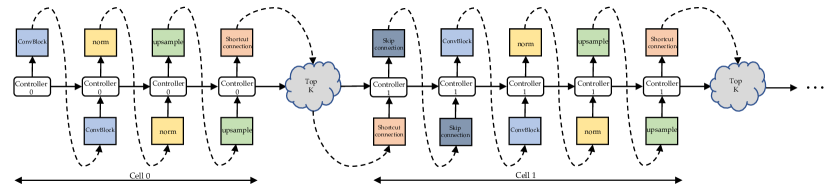
Figure 1: The running scheme of the RNN controller. At each time step, the controller outputs a hidden vector to be decoded into an operation, with its corresponding softmax classifier. Note that, using MLAS, we use a different controller for the search of each cell. Once the search process for one cell is done, the controller samples $M$ candidate architectures and then picks the top $K$ from them. The top $K$ architectures’ controller outputs will fed as the input of the next cell’s controller.

3.1 Search Space

AutoGAN is based on a multi-level architecture search strategy, where the generator is composed of several cells. Here we use a (s+5) element tuple $(skip_{1},...,skip_{s},C,N,U,SC)$ to categorize the $s$-th cell, where $s$ is the cell index starting at 0 (0-th cell doesn’t have $skip_{0}$ connection):

• $skip_{i}$ is a binary value indicating whether the current $s$-th cell takes a skip connection from the $(i-1)$-th cell as its input, $i=1,...,s$. Note that each cell could take multiple skip connections from other preceding cells.

• $C$ is the basic convolution block type, including pre-activation [16] and post-activation convolution block.

• $N$ stands for the normalization type of this block, including three options: batch normalization[21], instance normalization[55], and no normalization.

• $U$ stands for the upsampling operation which was standard in current image generation GANs, including bilinear upsampling, nearest neighbour upsampling, and stride 2 deconvolution.

• $SC$ is a binary value indicating the in-cell shortcut.

Fig. 2 illustrates the AutoGAN generator search space. The upsampling operation $U$ will also determine the upsample method of the skip-in feature map.

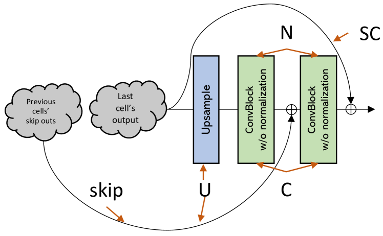
Figure 2: The search space of a generator cell in AutoGAN.

3.2 Proxy Task

Inception score (IS) [50] and FID score [18] are two main evaluation metrics for GANs. Since FID score is much more time-consuming to calculate, we choose the IS of each derived child model, as the reward to update controller via reinforcement learning.

Parameter sharing [40, 73] shows to effectively boost the efficiency of NAS [46]. Based on the parameter-sharing in [46], we further bring in a parameter dynamic-resetting strategy to AutoGAN. It has been observed that the training of GANs becomes unstable and undergoes mode collapse after long time training [5]. It could be a waste of time to continue training the shared collapsed model. Empirically, we observe the variance of the training loss (hinge loss) usually becomes very small when mode collapse happens.

Based on this observation, we set a moving window to store the most recent training loss values, for both generator and discriminator. Once the standard deviation of those stored training losses is smaller than a pre-defined threshold, the training of the shared GAN of current iteration will be terminated. The parameters of the shared-GAN model will be re-initialized after updating the controller at the current iteration. Notice that we do NOT re-initialize the parameters of the RNN controller, thus it could continue to guide the architecture search with inheriting the historic knowledge. With dynamic-resetting, the searching process becomes much more efficient.

3.3 Optimization Method

There are two sets of parameters in the AutoGAN: the RNN controller’s parameters (denoted as $\theta$); and the shared GAN parameters in the searched generator and the corresponding discriminator (denoted as $\omega$). The training process is briefly outlined in Algo. 1, as an alternating process between two phases.

The first phase will train $\omega$ of the shared GAN for several epochs, with $\theta$ fixed. For each training iteration of the shared GAN training process, a candidate architecture will be sampled by the RNN controller. Once the standard deviation of the recorded training loss drop below the threshold, the dynamic resetting FLAG $F_{DR}$ will be set to $True$ and the training process of shared GAN will be terminated immediately. Note that the shared GAN will not be re-initialized until the training of controller at the current epoch completes. The second phase trains $\theta$ with $\omega$ fixed: the controller will first sample $K$ child models of the shared generator. Their ISs will be calculated as rewards. The RNN controller will be updated via reinforcement learning with a moving average baseline. After training $u_{stage}$ iterations, the top $K$ architectures will be picked from the derived architectures. Meanwhile, a new controller will be initialized to proceed the architecture searching of next stage.

$\textnormal{{iters}}=0$ ;

$\textnormal{{stage}}=0$ ;

$F_{DR}=False$ ;

while  $\textnormal{{iters}}<90$  do

       train ($generator$, $discriminator$, $F_{DR}$);

       train ($controller$);

       if $\textnormal{{iters}}\quad\%\quad\textnormal{{$u_{stage}$}}==0$ then

             save the top $K$ architectures;

             $generator$ = grow ($generator$) ;

             $discriminator$ = grow ($discriminator$) ;

             $controller$ = new ($controller$);

             $\textnormal{{stage}}+=1$;

            

       end if

      if $F_{DR}==True$ then

             // dynamic reset

             initialize ($generator$);

             initialize ($discriminator$);

             $F_{DR}=False$;

            

       end if

      $\textnormal{{iters}}+=1$;

      

end while

Algorithm 1 Pseudo codes for AutoGAN searching.

3.3.1 Training Shared GAN

During this phase, we fix the RNN controller’s policy $\pi(\textbf{a},\theta)$ and update the shared parameters $\omega$ through standard GAN training. Specifically, we train with an alternating fashion using the hinge adversarial loss [42, 5, 53, 64]:

$$\begin{split}\mathcal{L}_{D}=&E_{x\sim q_{data}}[min(0,-1+D(x)]+\\ &E_{z\sim p(z)}[min(0,-1-D(G(z))],\end{split}$$ (1)

$$\mathcal{L}_{G}=E_{z\sim p(z)}[min(0,D(G(z))],$$ (2)

We further introduce multi-level architecture search (MLAS) to AutoGAN, where the generator (and correspondingly the discriminator) will grow progressively. MLAS performs the search in a bottom-up cell-wise fashion, using beam search [37]. When searching for the next cell, we will use a different controller, selects the top $K$ beams from current candidate cells and start the next round of search based on them.

3.3.2 Training the Controller

In this phase we fix $\omega$ and update the policy parameters $\theta$ of the controller. We define the reward $\mathcal{R}(a,\omega)$ as the IS of the sampled child model $a$. The RNN controller is updated using the Adam optimizer [28] via REINFORCE [59], with a moving average baseline. Besides, we also add a entropy term to encourage the exploration.

We use a LSTM [20] controller. For each time step, the LSTM will output a hidden vector, which will be decoded and classified by its corresponding softmax classifier. The LSTM controller works in an autogressive way, where the output of the last step will be fed into the next step. The operations of GAN’s each cell will be sampled from each time step’s output. Specifically, a new controller will be initialized when a new cell is added to the existing model to increase the output image resolution. The previous top $K$ models’ architectures and corresponding hidden vectors will be saved. Their hidden vectors will be fed into the new controller as input to search for next cell’s operations.

3.3.3 Architecture Derivation

We will first sample several generator architectures from the learned policy $\pi(\textbf{a},\theta)$. Then, the reward $R$ (Inception score) will be calculated for each model. We will then pick top $K$ models in terms of highest rewards, and train them from scratch. After that, we evaluate their Inception scores again, and the model with the highest Inception score becomes our final derived generator architecture.

4 Experiments

Datasets

In this paper, we adopt CIFAR-10 [29] as the main testbed for AutoGAN. It consists of 50,000 training image and 10,000 test images, where each image is of $32\times 32$ resolution. We use the training set to train AutoGAN, without any data augmentation.

We also adopt the STL-10 dataset to show the transferablity of AutoGAN discovered architectures. When using STL-10 for training, we adopt both the 5,000 image training set and 100,000 image unlabeled set. All images are resized to $48\times 48$, without any other data augmentation.

Training details

We follow the training setting of spectral normalization GAN [42] when training the shared GAN. The learning rate of both generator and discriminator are set to $210-4$, using the hinge loss, an Adam optimizer [28], a batch size of 64 for discriminator and a batch size of 128 for generator. The spectral normalization is only enforced on the discriminator. We train our controller using Adam [28], with learning rate of $3.510-4$. We also add the entropy of the controller’s output probability to the reward, weighted by $110-4$, in order to encourage the exploration.

AutoGAN is searched for 90 iterations. For each iteration, the shared GAN will be trained for 15 epochs, and the controller will be trained for 30 steps. We set the dynamic-resetting variance threshold at $110-3$. We train the discovered architectures, using the same training setting as the shared GAN, for 50,000 generator iterations.

4.1 Results on CIFAR 10

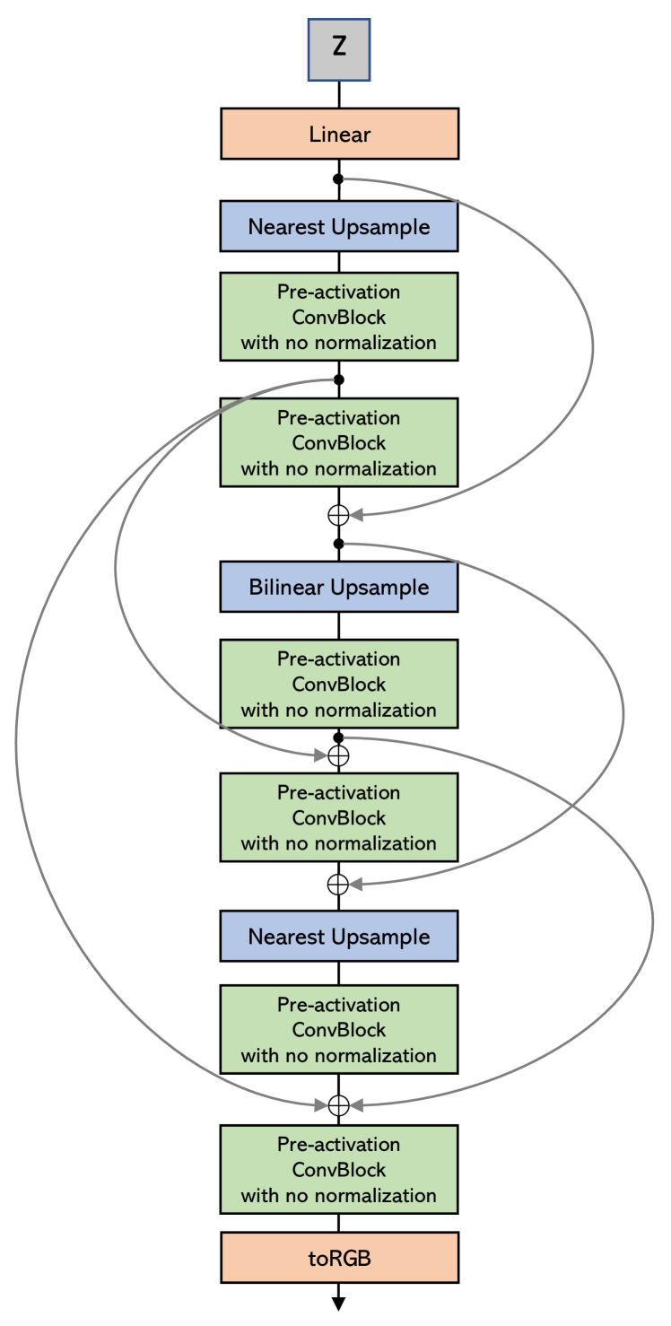
Figure 3: The AutoGAN (generator) architecture discovered by AutoGAN on CIFAR-10.

The generator architecture discovered by AutoGAN on the CIFAR-10 training set is displayed in Fig. 3. For the task of unconditional CIFAR-10 image generation (no class labels used), a number of notable observations could be summarized:

• The discovered architecture has 3 convolution blocks. AutoGAN clearly prefers pre-activation convolution block, than post-activation convolution block.

• AutoGAN highly prefers nearest neighbour upsample (also bilinear upsample) to deconvolution. That seems to coincide with previous experience [45] that deconvolution might give rise to checkboard artifacts and nearest neighbour might thus be more favored.

• Interestingly enough, AutoGAN seems to prefer not using any normalization.

• AutoGAN is clearly in favor of (denser) skipping connections. Especially, it is able to discover medium and long skips (skipping 2 - 4 convolutional layers), achieving multi-scale feature fusion.

We compare AutoGAN with recently published results by hand-crafted GANs on the CIFAR-10 dataset, in Table 2. All results are collected from those original papers: therefore, they are obtained under their hand-tuned, best possible training settings. In terms of inception score, AutoGAN is slightly next to Progressive GAN [26], and surpasses many latest strong competitors such as SN-GAN [42], improving MMD-GAN [56], Dist-GAN [54], MGAN [19], and WGAN-GP [13]. In terms of FID, AutoGAN outperforms all current state-of-the-art models. The visual examples of CIFAR-10 generated results are shown in Fig. 4.

Note that the current search space of AutoGAN can only cover SN-GAN, but not the others; for example, WGAN-GP used the Wasserstein loss (with gradient clipping), and MGAN adopts a multi-discriminator structure (while our discriminator is very plain and not searched). By using the same group of building blocks, AutoGAN is able to outperform the hand-crafted SN-GAN: that fair comparison presents direct evidence for both the importance of generator structure, and the effectiveness of our search algorithm.

Although not equipped with any explicit model complexity regularization yet, AutoGAN demonstrates the expected model parameter efficiency from NAS. The top discovered architecture in Fig. 3 has 1.77G FLOPs, while its performance is clearly better than SN-GAN (1.69G FLOPs) and comparable to Progressive GAN (6.39G FLOPs).

Table 1: Inception score and FID score of unconditional image generation task on CIFAR-10. We achieve a state-of-the-art FID score of 12.42

Method	Inception score	FID
DCGAN[47]	$6.64\pm.14$	-
Improved GAN[50]	$6.86\pm.06$	-
LRGAN [62]	$7.17\pm.17$	-
DFM[58]	$7.72\pm.13$	-
ProbGAN[14]	7.75	24.60
WGAN-GP, ResNet [13]	$7.86\pm.07$	-
Splitting GAN [12]	$7.90\pm.09$	-
SN-GAN [42]	$8.22\pm.05$	$21.7\pm.01$
MGAN[19]	$8.33\pm.10$	26.7
Dist-GAN [54]	-	$17.61\pm.30$
Progressive GAN [26]	8.80 $\pm$ .05	-
Improving MMD GAN [56]	8.29	16.21
AutoGAN-top1 (Ours)	$8.55\pm.10$	12.42
AutoGAN-top2	$8.42\pm.07$	$13.67$
AutoGAN-top3	$8.41\pm.11$	$13.87$

Figure 4: The generated CIFAR-10 results of AutoGAN. They are randomly sampled rather than cherry-picked.

We also report the Inception score and FID score of the candidate top 2 and top 3 discovered architectures in the bottom of Tab. 2. Their corresponding architectures are shown in Fig. 5. We can see all of our top 3 discovered architecture achieves competitive performance with current state-of-the-art models.

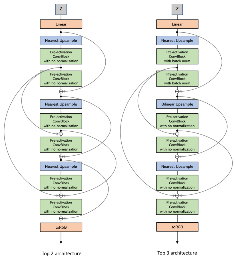
Figure 5: The top 2 and top 3 discovered architectures.

4.2 Transferability on STL-10

The next question that we try to answer is: might the discovered architecture overfit the dataset? In other words, would the same architecture stay powerful, when we use another dataset to re-train its weights (with the architecture structure fixed)? To address this question, we take the AutoGAN-discovered architecture on CIFAR-10, and re-train its weights on the STL-10 training and unlabled set, for the unconditional image generation task on STL-10. Note that STL-10 has higher image resolution than CIFAR-10.

We compare with recently published results by hand-crafted GANs on the STL-10 dataset, in Table 2. Our result turns out to be surprisingly encouraging: while AutoGAN slightly lags behinds improving MMD-GAN in terms of inception score, it achieves the best FID result of 31.01 among all. The visual examples of STL-10 generated results are shown in Fig. 4. We expect to achieve even superior results on STL-10 if we re-perform the architecture search from the scratch, and leave it for future work.

Table 2: Inception score and FID score with unconditional image generation on STL-10. AutoGAN uses the discovered architecture on CIFAR-10.

Method	Inception score	FID
D2GAN [44]	$7.98$	-
DFM [58]	$8.51\pm.13$	-
ProbGAN[14]	$8.87\pm.095$	$46.74$
SN-GAN [42]	$9.10\pm.04$	$40.1\pm.50$
Dist-GAN [54]	-	36.19
Improving MMD GAN [56]	9.34	37.63
AutoGAN (Ours)	$9.16\pm.12$	31.01

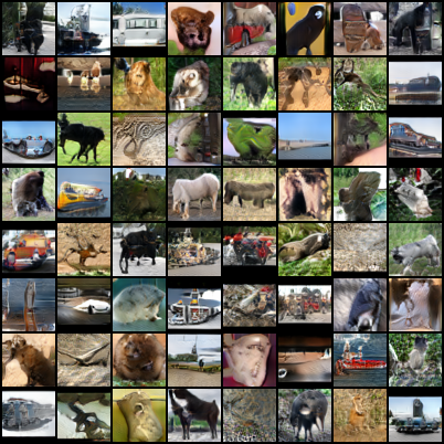
Figure 6: The generated STL-10 results of AutoGAN. They are randomly sampled rather than cherry-picked.

4.3 Ablation Study and Analysis

4.3.1 Validation of Proxy tasks

The proxy task of our method is to directly evaluate IS on the child model of the shared GAN, which boosts the training speed dramatically. To validate the effectiveness of the designed proxy task, we train the derived architectures from scratch for 30 epochs and evaluate their IS, using AutoGAN on CFIAR-10. We plot the correlation between the evaluation value provided by our proxy task (Proxy) and the true evaluation (Real) in Fig. 7. We can observe a positive correlation between each other, with a Spearman’s rank correlation coefficient of 0.779, demonstrating that the proxy task provides a fair approximation of the true evaluation. We can also observe that the proxy evaluation tends to underestimate the Inception score, because of the uncompleted and shared training in our proxy task.

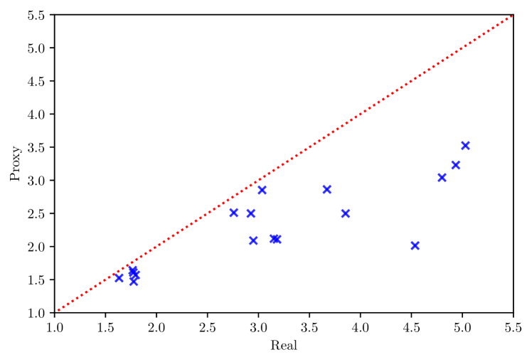
Figure 7: The correlation plot of real evaluation and proxy task performance on CIFAR-10.

4.3.2 Comparing to Using FID as Reward

Besides IS, another important evaluation metric for GAN is the FID score [50]: the smaller FID indicates better generation quality. What if we use the reciprocal of FID, instead of IS, as the AutoGAN controller’s reward? To answer this question, on CIFAR-10, we search for another model from scratch, using the reciprocal of FID as the reward (everything else unchanged), and compare to the AutoGAN trained with IS reward. During searching, for both models, we evaluate both IS and FID values periodically with the training progressing. Fig. 8 plots the curves, from which we can see that while both rewards can increase as the search goes on, the FID-driven search (red curves) shows comparable performance with the IS-driven search (blue curves), under both metrics. However, computing FID is more time-consuming than calculating IS, as it requires to calculate the co-variance and mean of large matrices. Thus, we choose IS as the default reward for AutoGAN.

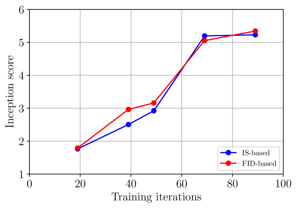
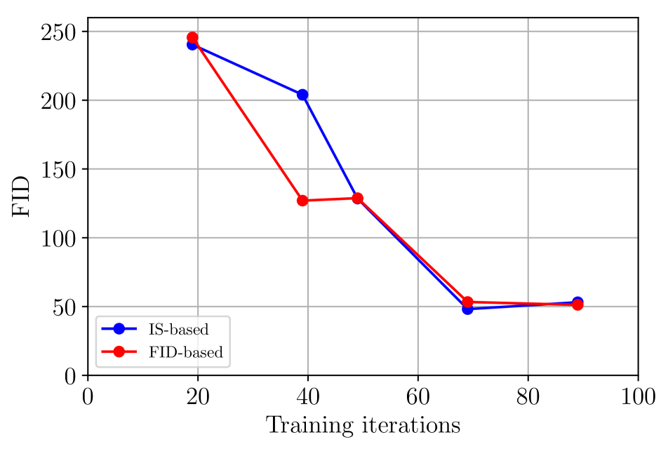
Figure 8: Comparison between using IS and FID (reciprocal) as the AutoGAN’s reward. The model with IS-based reward is plotted in blue, while the one with FID-based reward in red. The top figure shows both models’ IS values as training goes on, while the bottom presents FID values.

4.3.3 Parameter dynamic-resetting

It is well known that the training process of GAN is extremely unstable and prone to mode collapse [5] after long time training. It could be a waste of time to continue training the shared collapsed model. Hence, we introduce parameter dynamic-resetting to alleviate the issue. For comparison, we conduct two AutoGAN experiments on CIFAR-10, with the parameter sharing strategy proposed in [46], and our proposed dynamic-resetting plus parameter sharing strategy. We evaluate IS during both training processes. As plotted in Figure 9, we can see that they achieve comparable performance. However, the training process with dynamic-resetting only takes 43 hours, while it will take 72 hours without dynamic-resetting.

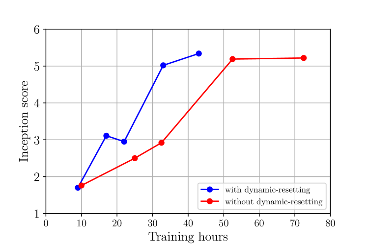
Figure 9: Comparing AutoGAN with (blue) and without (red) dynamic-resetting. Dynamic-resetting can boost training efficiency while achieving comparable performace.

4.3.4 Multi-Level Architecture Search

Our AutoGAN framework employs a multi-level architecture search (MLAS) strategy by default. For comparison, we conduct another AutoGAN experiment on CIFAR-10 with single-level architecture search (SLAS), where the whole architecture will be derived through a single controller at once. We evaluate ISs and compare with the training with MLAS. We can see that SLAS obtain high Inception score at the beginning, but the Inception score of MLAS grows progressively and finally outperforms SLAS. Besides, Training SLAS is much slower than training MLAS, as the generator output image will always be of the final resolution. Figure 10 demonstrates the evident and consistent advantages of MLAS.

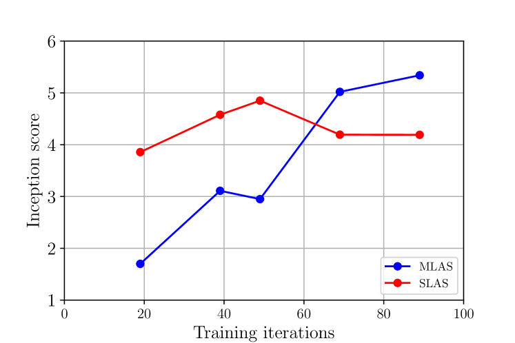
Figure 10: Comparison of AutoGAN with MLAS (blue line) and SLAS (red line) training chemes.

4.3.5 Comparison to random search

We implemented the two random search algorithms in [34]: one with weight sharing and the other without weight sharing (early stopping). We re-searched AutoGAN with these two algorithms on CIFAR-10 and constrained the searching time for 48 hours. As a result, the discovered architecture with weight sharing achieves IS = 8.09 and FID = 17.34, while the other achieves IS = 7.97 and FID = 21.39. Both are inferior to our proposed search algorithm and endorse its effectiveness.

5 Conclusions, Limitations and Discussions

AutoGAN presents the first effort on bringing NAS into GANs. It is able to identify highly effective architectures on both CIFAR-10 and STL-10 datasets, achieving competitive image generation results against current state-of-the-art, hand-crafted GAN models. The ablation study further reveals the benefit of each component.

AutoGAN appears to be more challenging than NAS for image classification, due to the high instability and hyperparameter sensitivity of GAN training itself. Recall that at the initial stage of AutoML, it can only design small neural networks that perform on par with neural networks designed by human experts, and these results were constrained to small academic datasets such as CIFAR-10 and Penn Treebank [71]. Likewise, despite its preliminary success and promise, there is undoubtedly a large room for AutoGAN to improve.

In order to make AutoGAN further more competitive than state-of-the-art hand-designed GANs, we point out a few specific items that call for continuing efforts:

• The current search space of AutoGAN is limited, and some powerful GANs are excluded from the searchable range. It needs to be enlarged with more building blocks, that prove to be effective in the GAN literature. Referring to recent GAN benchmark studies [39, 32], we consider extending our search space with the attention/self-attention [64], the style-based generator [27], the relativistic discriminator [25] and various losses such as the Wasserstein loss [3], among others.

• We have not yet tested AutoGAN on higher-resolution image synthesis so far, e.g. ImageNet. While the same algorithm is directly applicable in principle, the computational cost would become prohibitively high. For example, the search on CIFAR-10 already takes 43 hours. The key challenge lies in how to further improve the search algorithm efficiency.

  As one possible strategy, NAS in image classification typically applies transfer learning from low-resolution images to higher resolutions [72]. It may be interesting, though challenging, to see how the similar idea will be applied to the image generation task of GANs, since it will be more demanding in preserving/synthesizing details than classification.

• We have not unleashed the potential of searching for better discriminators. We might formulate an alternating search between the generator and the discriminator, which can turn AutoGAN even far more challenging.

• Eventually, AutoGAN will need the capability to incorporate labels, such as conditional GANs [41] and semi-supervised GANs [50].

References

- [1] Karim Ahmed and Lorenzo Torresani. MaskConnect - Connectivity Learning by Gradient Descent. ECCV, cs.CV, 2018.
- [2] Martin Arjovsky and Léon Bottou. Towards principled methods for training generative adversarial networks. arXiv preprint arXiv:1701.04862, 2017.
- [3] Martin Arjovsky, Soumith Chintala, and Léon Bottou. Wasserstein generative adversarial networks. In International Conference on Machine Learning, pages 214–223, 2017.
- [4] Bowen Baker, Otkrist Gupta, Nikhil Naik, and Ramesh Raskar. Designing neural network architectures using reinforcement learning. arXiv preprint arXiv:1611.02167, 2016.
- [5] Andrew Brock, Jeff Donahue, and Karen Simonyan. Large scale gan training for high fidelity natural image synthesis. arXiv preprint arXiv:1809.11096, 2018.
- [6] Andrew Brock, Theodore Lim, James M Ritchie, and Nick Weston. Neural photo editing with introspective adversarial networks. arXiv preprint arXiv:1609.07093, 2016.
- [7] Liang-Chieh Chen, Maxwell Collins, Yukun Zhu, George Papandreou, Barret Zoph, Florian Schroff, Hartwig Adam, and Jon Shlens. Searching for efficient multi-scale architectures for dense image prediction. In Advances in Neural Information Processing Systems, pages 8713–8724, 2018.
- [8] Liang-Chieh Chen, George Papandreou, Iasonas Kokkinos, Kevin Murphy, and Alan L Yuille. Deeplab: Semantic image segmentation with deep convolutional nets, atrous convolution, and fully connected crfs. IEEE transactions on pattern analysis and machine intelligence, 40(4):834–848, 2018.
- [9] Liang-Chieh Chen, George Papandreou, Florian Schroff, and Hartwig Adam. Rethinking atrous convolution for semantic image segmentation. arXiv preprint arXiv:1706.05587, 2017.
- [10] Patryk Chrabaszcz, Ilya Loshchilov, and Frank Hutter. A downsampled variant of imagenet as an alternative to the cifar datasets. arXiv preprint arXiv:1707.08819, 2017.
- [11] Ian Goodfellow, Jean Pouget-Abadie, Mehdi Mirza, Bing Xu, David Warde-Farley, Sherjil Ozair, Aaron Courville, and Yoshua Bengio. Generative adversarial nets. In Advances in neural information processing systems, pages 2672–2680, 2014.
- [12] Guillermo L Grinblat, Lucas C Uzal, and Pablo M Granitto. Class-splitting generative adversarial networks. arXiv preprint arXiv:1709.07359, 2017.
- [13] Ishaan Gulrajani, Faruk Ahmed, Martin Arjovsky, Vincent Dumoulin, and Aaron C Courville. Improved training of wasserstein gans. In Advances in Neural Information Processing Systems, pages 5767–5777, 2017.
- [14] Guang-He Lee Yonglong Tian Hao He, Hao Wang. Probgan: Towards probabilistic gan with theoretical guarantees. In ICLR, 2019.
- [15] Kaiming He, Xiangyu Zhang, Shaoqing Ren, and Jian Sun. Deep residual learning for image recognition. In Proceedings of the IEEE conference on computer vision and pattern recognition, pages 770–778, 2016.
- [16] Kaiming He, Xiangyu Zhang, Shaoqing Ren, and Jian Sun. Identity mappings in deep residual networks. In European conference on computer vision, pages 630–645. Springer, 2016.
- [17] Yihui He, Ji Lin, Zhijian Liu, Hanrui Wang, Li-Jia Li, and Song Han. Amc: Automl for model compression and acceleration on mobile devices. In European Conference on Computer Vision, pages 815–832. Springer, 2018.
- [18] Martin Heusel, Hubert Ramsauer, Thomas Unterthiner, Bernhard Nessler, Günter Klambauer, and Sepp Hochreiter. Gans trained by a two time-scale update rule converge to a nash equilibrium. arXiv preprint arXiv:1706.08500, 12(1), 2017.
- [19] Quan Hoang, Tu Dinh Nguyen, Trung Le, and Dinh Phung. Mgan: Training generative adversarial nets with multiple generators. 2018.
- [20] Sepp Hochreiter and Jürgen Schmidhuber. Long short-term memory. Neural computation, 9(8):1735–1780, 1997.
- [21] Sergey Ioffe and Christian Szegedy. Batch normalization: Accelerating deep network training by reducing internal covariate shift. arXiv preprint arXiv:1502.03167, 2015.
- [22] Phillip Isola, Jun-Yan Zhu, Tinghui Zhou, and Alexei A Efros. Image-to-image translation with conditional adversarial networks. In 2017 IEEE Conference on Computer Vision and Pattern Recognition (CVPR), pages 5967–5976. IEEE, 2017.
- [23] Yifan Jiang, Xinyu Gong, Ding Liu, Yu Cheng, Chen Fang, Xiaohui Shen, Jianchao Yang, Pan Zhou, and Zhangyang Wang. Enlightengan: Deep light enhancement without paired supervision. arXiv preprint arXiv:1906.06972, 2019.
- [24] Haifeng Jin, Qingquan Song, and Xia Hu. Auto-keras: Efficient neural architecture search with network morphism, 2018.
- [25] Alexia Jolicoeur-Martineau. The relativistic discriminator: a key element missing from standard gan. arXiv preprint arXiv:1807.00734, 2018.
- [26] Tero Karras, Timo Aila, Samuli Laine, and Jaakko Lehtinen. Progressive growing of gans for improved quality, stability, and variation. ICLR, 2018.
- [27] Tero Karras, Samuli Laine, and Timo Aila. A style-based generator architecture for generative adversarial networks. arXiv preprint arXiv:1812.04948, 2018.
- [28] Diederik P Kingma and Jimmy Ba. Adam: A method for stochastic optimization. arXiv preprint arXiv:1412.6980, 2014.
- [29] Alex Krizhevsky and Geoffrey Hinton. Learning multiple layers of features from tiny images. Technical report, Citeseer, 2009.
- [30] Alex Krizhevsky, Ilya Sutskever, and Geoffrey E Hinton. Imagenet classification with deep convolutional neural networks. In Advances in neural information processing systems, pages 1097–1105, 2012.
- [31] Orest Kupyn, Volodymyr Budzan, Mykola Mykhailych, Dmytro Mishkin, and Jiří Matas. Deblurgan: Blind motion deblurring using conditional adversarial networks. In Proceedings of the IEEE Conference on Computer Vision and Pattern Recognition, pages 8183–8192, 2018.
- [32] Karol Kurach, Mario Lucic, Xiaohua Zhai, Marcin Michalski, and Sylvain Gelly. The gan landscape: Losses, architectures, regularization, and normalization. arXiv preprint arXiv:1807.04720, 2018.
- [33] Christian Ledig, Lucas Theis, Ferenc Huszár, Jose Caballero, Andrew Cunningham, Alejandro Acosta, Andrew Aitken, Alykhan Tejani, Johannes Totz, Zehan Wang, et al. Photo-realistic single image super-resolution using a generative adversarial network. In 2017 IEEE Conference on Computer Vision and Pattern Recognition (CVPR), pages 105–114. IEEE, 2017.
- [34] Liam Li and Ameet Talwalkar. Random search and reproducibility for neural architecture search. arXiv, 2019.
- [35] Tsung-Yi Lin, Piotr Dollár, Ross Girshick, Kaiming He, Bharath Hariharan, and Serge Belongie. Feature pyramid networks for object detection. In CVPR, volume 1, page 4, 2017.
- [36] Chenxi Liu, Liang-Chieh Chen, Florian Schroff, Hartwig Adam, Wei Hua, Alan Yuille, and Li Fei-Fei. Auto-deeplab: Hierarchical neural architecture search for semantic image segmentation. arXiv preprint arXiv:1901.02985, 2019.
- [37] Chenxi Liu, Barret Zoph, Maxim Neumann, Jonathon Shlens, Wei Hua, Li-Jia Li, Li Fei-Fei, Alan Yuille, Jonathan Huang, and Kevin Murphy. Progressive Neural Architecture Search. pages 19–34, 2018.
- [38] H Liu, K Simonyan, Y Yang arXiv preprint arXiv 1806.09055, and 2018. Darts: Differentiable architecture search. arxiv.org.
- [39] Mario Lucic, Karol Kurach, Marcin Michalski, Sylvain Gelly, and Olivier Bousquet. Are gans created equal? a large-scale study. In Advances in neural information processing systems, pages 700–709, 2018.
- [40] Minh-Thang Luong, Quoc V Le, Ilya Sutskever, Oriol Vinyals, and Lukasz Kaiser. Multi-task sequence to sequence learning. arXiv preprint arXiv:1511.06114, 2015.
- [41] Mehdi Mirza and Simon Osindero. Conditional generative adversarial nets. arXiv preprint arXiv:1411.1784, 2014.
- [42] Takeru Miyato, Toshiki Kataoka, Masanori Koyama, and Yuichi Yoshida. Spectral normalization for generative adversarial networks. arXiv preprint arXiv:1802.05957, 2018.
- [43] Alejandro Newell, Kaiyu Yang, and Jia Deng. Stacked hourglass networks for human pose estimation. In European Conference on Computer Vision, pages 483–499. Springer, 2016.
- [44] Tu Nguyen, Trung Le, Hung Vu, and Dinh Phung. Dual discriminator generative adversarial nets. In Advances in Neural Information Processing Systems, pages 2670–2680, 2017.
- [45] Augustus Odena, Vincent Dumoulin, and Chris Olah. Deconvolution and checkerboard artifacts. Distill, 1(10):e3, 2016.
- [46] H Pham, M Y Guan, B Zoph, Q V Le, J Dean arXiv preprint arXiv, and 2018. Efficient Neural Architecture Search via Parameter Sharing. arxiv.org.
- [47] Alec Radford, Luke Metz, and Soumith Chintala. Unsupervised representation learning with deep convolutional generative adversarial networks. arXiv preprint arXiv:1511.06434, 2015.
- [48] S Reed, Z Akata, X Yan, L Logeswaran arXiv preprint arXiv, and 2016. Generative adversarial text to image synthesis. jmlr.org, 2016.
- [49] Olaf Ronneberger, Philipp Fischer, and Thomas Brox. U-net: Convolutional networks for biomedical image segmentation. In International Conference on Medical image computing and computer-assisted intervention, pages 234–241. Springer, 2015.
- [50] Tim Salimans, Ian Goodfellow, Wojciech Zaremba, Vicki Cheung, Alec Radford, and Xi Chen. Improved techniques for training gans. In Advances in Neural Information Processing Systems, pages 2234–2242, 2016.
- [51] Christian Szegedy, Wei Liu, Yangqing Jia, Pierre Sermanet, Scott Reed, Dragomir Anguelov, Dumitru Erhan, Vincent Vanhoucke, and Andrew Rabinovich. Going deeper with convolutions. In Proceedings of the IEEE conference on computer vision and pattern recognition, pages 1–9, 2015.
- [52] Christian Szegedy, Vincent Vanhoucke, Sergey Ioffe, Jon Shlens, and Zbigniew Wojna. Rethinking the inception architecture for computer vision. In Proceedings of the IEEE conference on computer vision and pattern recognition, pages 2818–2826, 2016.
- [53] Dustin Tran, Rajesh Ranganath, and David M Blei. Deep and hierarchical implicit models. CoRR, abs/1702.08896, 2017.
- [54] Ngoc-Trung Tran, Tuan-Anh Bui, and Ngai-Man Cheung. Dist-gan: An improved gan using distance constraints. In Proceedings of the European Conference on Computer Vision (ECCV), pages 370–385, 2018.
- [55] Dmitry Ulyanov, Andrea Vedaldi, and Victor Lempitsky. Instance normalization: The missing ingredient for fast stylization. arXiv preprint arXiv:1607.08022, 2016.
- [56] Wei Wang, Yuan Sun, and Saman Halgamuge. Improving mmd-gan training with repulsive loss function. arXiv preprint arXiv:1812.09916, 2018.
- [57] Zhangyang Wang, Shiyu Chang, Yingzhen Yang, Ding Liu, and Thomas S Huang. Studying very low resolution recognition using deep networks. In Proceedings of the IEEE Conference on Computer Vision and Pattern Recognition, pages 4792–4800, 2016.
- [58] David Warde-Farley and Yoshua Bengio. Improving generative adversarial networks with denoising feature matching.(2017). In ICLR, 2017.
- [59] Ronald J Williams. Simple statistical gradient-following algorithms for connectionist reinforcement learning. Machine learning, 8(3-4):229–256, 1992.
- [60] Lingxi Xie and Alan Yuille. Genetic cnn. In 2017 IEEE International Conference on Computer Vision (ICCV), pages 1388–1397. IEEE, 2017.
- [61] Tao Xu, Pengchuan Zhang, Qiuyuan Huang, Han Zhang, Zhe Gan, Xiaolei Huang, and Xiaodong He. Attngan: Fine-grained text to image generation with attentional generative adversarial networks. arXiv preprint, 2017.
- [62] Jianwei Yang, Anitha Kannan, Dhruv Batra, and Devi Parikh. Lr-gan: Layered recursive generative adversarial networks for image generation. arXiv preprint arXiv:1703.01560, 2017.
- [63] Shuai Yang, Zhangyang Wang, Zhaowen Wang, Ning Xu, Jiaying Liu, and Zongming Guo. Controllable artistic text style transfer via shape-matching gan. arXiv preprint arXiv:1905.01354, 2019.
- [64] Han Zhang, Ian Goodfellow, Dimitris Metaxas, and Augustus Odena. Self-attention generative adversarial networks. arXiv preprint arXiv:1805.08318, 2018.
- [65] Han Zhang, Tao Xu, Hongsheng Li, Shaoting Zhang, Xiaogang Wang, Xiaolei Huang, and Dimitris Metaxas. Stackgan++: Realistic image synthesis with stacked generative adversarial networks. arXiv preprint arXiv:1710.10916, 2017.
- [66] Han Zhang, Tao Xu, Hongsheng Li, Shaoting Zhang, Xiaogang Wang, Xiaolei Huang, and Dimitris N Metaxas. Stackgan: Text to photo-realistic image synthesis with stacked generative adversarial networks. In Proceedings of the IEEE International Conference on Computer Vision, pages 5907–5915, 2017.
- [67] Xiaofeng Zhang, Zhangyang Wang, Dong Liu, and Qing Ling. Dada: Deep adversarial data augmentation for extremely low data regime classification. In ICASSP 2019-2019 IEEE International Conference on Acoustics, Speech and Signal Processing (ICASSP), pages 2807–2811. IEEE, 2019.
- [68] Junbo Zhao, Michael Mathieu, and Yann LeCun. Energy-based generative adversarial network. arXiv preprint arXiv:1609.03126, 2016.
- [69] Zhao Zhong, Junjie Yan, Wei Wu, Jing Shao, and Cheng-Lin Liu. Practical block-wise neural network architecture generation. In Proceedings of the IEEE Conference on Computer Vision and Pattern Recognition, pages 2423–2432, 2018.
- [70] Jun-Yan Zhu, Taesung Park, Phillip Isola, and Alexei A Efros. Unpaired Image-to-Image Translation using Cycle-Consistent Adversarial Networks. arXiv.org, Mar. 2017.
- [71] Barret Zoph and Quoc V Le. Neural architecture search with reinforcement learning. arXiv preprint arXiv:1611.01578, 2016.
- [72] Barret Zoph, Vijay Vasudevan, Jonathon Shlens, and Quoc V Le. Learning Transferable Architectures for Scalable Image Recognition. CVPR, 2018.
- [73] Barret Zoph, Deniz Yuret, Jonathan May, and Kevin Knight. Transfer learning for low-resource neural machine translation. arXiv preprint arXiv:1604.02201, 2016.