Fixation probabilities in evolutionary dynamics under weak selection

Abstract

In evolutionary dynamics, a key measure of a mutant trait’s success is the probability that it takes over the population given some initial mutant-appearance distribution. This “fixation probability” is difficult to compute in general, as it depends on the mutation’s effect on the organism as well as the population’s spatial structure, mating patterns, and other factors. In this study, we consider weak selection, which means that the mutation’s effect on the organism is small. We obtain a weak-selection perturbation expansion of a mutant’s fixation probability, from an arbitrary initial configuration of mutant and resident types. Our results apply to a broad class of stochastic evolutionary models, in which the size and spatial structure are arbitrary (but fixed). The problem of whether selection favors a given trait is thereby reduced from exponential to polynomial complexity in the population size, when selection is weak. We conclude by applying these methods to obtain new results for evolutionary dynamics on graphs.

1 Introduction

Many studies of stochastic evolutionary dynamics concern the competition of two types (traits) in a finite population. Through a series of births and deaths, the composition of the population changes over time. Absent recurring mutation, one of the two types will eventually become fixed and the other will go extinct. Such models may incorporate frequency-dependent selection as well as spatial structure or other forms of population structure. The fundamental question is to identify the selective differences that favor the fixation of one type over the other.

This question is typically answered by computing a trait’s fixation probability (Haldane, 1927; Moran, 1958; Kimura, 1962; Patwa and Wahl, 2008; Traulsen and Hauert, 2010; Der et al., 2011; Hindersin and Traulsen, 2014; McCandlish et al., 2015; Hindersin et al., 2016) as a function of the initial configuration of the two types. Direct calculation of a mutant’s fixation probability is possible in simple models of well-mixed populations (Moran, 1958; Taylor et al., 2004) or spatially structured populations that are highly symmetric (Lieberman et al., 2005; Broom and Rychtář, 2008; Hindersin and Traulsen, 2014) or small (Hindersin and Traulsen, 2015; Cuesta et al., 2018; Möller et al., 2019; Tkadlec et al., 2019). For large populations, fixation probabilities can sometimes be approximated using diffusion methods (Kimura, 1962; Roze and Rousset, 2003; Ewens, 2004; Chen, 2018).

When selection is weak, perturbative methods can be applied to the computation of fixation probabilities (Haldane, 1927; Nowak et al., 2004; Lessard and Ladret, 2007). The first-order effects of selection on fixation probabilities provide information about whether selection favors one trait over another, and, if so, by how much. This perturbative approach is often paired with methods from coalescent theory (Rousset, 2003; Chen, 2013; Van Cleve, 2015; Chen et al., 2016; Allen et al., 2017, 2020).

Our aim in this work is to generalize the weak-selection method for computing fixation probability to a broad class of evolutionary models. Our main result is a first-order weak-selection expansion of a mutant’s fixation probability from any initial condition. This result applies to arbitrary forms of spatial structure and frequency-dependent selection, and the expansion can be computed for any particular model and initial configuration by solving a system of linear equations. Under conditions that apply to most models of interest, the size of this system—and hence the complexity of computing this expansion—exhibits polynomial growth in the population size.

Our approach is based on a modeling framework developed by Allen and Tarnita (2014) and Allen and McAvoy (2019), which is described in Section 2. This framework describes stochastic trait transmission in a population of fixed size, $N$, and spatial structure. This setup leads to a finite Markov chain model of selection. Special cases of this framework include the Moran (Moran, 1958) and Wright-Fisher models (Fisher, 1930; Wright, 1931; Imhof and Nowak, 2006), as well as evolutionary games in graph-structured populations (Ohtsuki et al., 2006; Szabó and Fáth, 2007; Nowak et al., 2009; Allen et al., 2017). We use this framework to define the degree of an evolutionary process, which later plays an important role in determining the computational complexity of calculating fixation probabilities.

In Section 3, we establish a connection between sojourn times and stationary probabilities. Specifically, we compare the original Markov chain, which is absorbing, to an amended Markov chain, in which the initial configuration $\bm{\xi}$ can be re-established from the all-$A$ and all-$B$ states with some probability, $u$. This amended Markov chain is recurrent, and it has a unique stationary distribution. We show that sojourn times for transient states of the original Markov chain are equal to $u$-derivatives, at $u=0$, of stationary probabilities in the amended chain. We also define a set-valued coalescent process that is used in the proof of our main results.

Section 4 proves our main result regarding fixation probabilities. We consider the fixation probability, $\rho_{A}\left(\bm{\xi}\right)$, of type $A$ in a population whose initial configuration of $A$ and $B$ is $\bm{\xi}$. The intensity of selection, $\delta$, which quantifies selective differences between the two types, is assumed to be sufficiently weak, meaning $\delta\ll 1$. Our main result is a formula for calculating $\rho_{A}\left(\bm{\xi}\right)$ to first order in the selection intensity $\delta$. This formula depends on the first-order effects of selection on marginal trait-transmission probabilities together with a set of sojourn times for neutral drift. The latter can be evaluated by solving a linear system of size $O\left(N^{D+1}\right)$, where $D$ is the degree of the process. This linear system is what bounds the complexity in $N$ of calculating the first-order coefficient, $\frac{d}{d\delta}\Big{|}_{\delta=0}\rho_{A}\left(\bm{\xi}\right)$.

In Section 5, we extend our main result to the case that the initial configuration of $A$ and $B$ is stochastic rather than deterministic. We derive a formula for $\frac{d}{d\delta}\Big{|}_{\delta=0}\operatorname{\mathbb{E}}_{\mu_{A}}\left[\rho_{A}\right]$, where $\mu_{A}$ is an arbitrary distribution over initial configurations of $A$ and $B$ (and which can also depend on $\delta$). Section 6 considers relative measures of evolutionary success (Tarnita and Taylor, 2014) obtained by comparing $\operatorname{\mathbb{E}}_{\mu_{A}}\left[\rho_{A}\right]$ to $\operatorname{\mathbb{E}}_{\mu_{B}}\left[\rho_{B}\right]$ when $A$ and $B$ each have their own initial distributions, $\mu_{A}$ and $\mu_{B}$.

Finally, we apply our results to several well-known questions in evolutionary dynamics, particularly on graph-structured populations. Section 7 discusses the case of constant fecundity, wherein the reproductive rate of an individual depends on only its own type. A large body of research (Lieberman et al., 2005; Broom and Rychtář, 2008; Broom et al., 2011; Voorhees, 2013; Monk et al., 2014; Hindersin and Traulsen, 2015; Kaveh et al., 2015; Cuesta et al., 2017; Pavlogiannis et al., 2018; Möller et al., 2019; Tkadlec et al., 2019) aims to understand the effects of graph structure on fixation probabilities in this context. Our results provide efficient recipes to calculate fixation probabilities under weak selection. Section 8 turns to evolutionary game theory. For a particular prisoner’s dilemma game (the “donation game”; Sigmund, 2010), we derive a formula for the fixation probability of cooperation from any starting configuration on an arbitrary weighted graph, generalizing and unifying a number of earlier results (Ohtsuki et al., 2006; Taylor et al., 2007; Chen, 2013; Allen and Nowak, 2014; Chen et al., 2016; Allen et al., 2017).

2 Modeling evolutionary dynamics

We employ a framework previously developed by Allen and Tarnita (2014) and Allen and McAvoy (2019) to represent an evolving population with arbitrary forms of spatial structure and frequency dependence. In addition to being described below, all of the notation and symbols we use are outlined in Table LABEL:tab:notationtable. Although we will use the language of a haploid asexual population, our formalism applies equally well to diploid, haplodiploid, or other populations by considering the alleles to be asexual replicators (the “gene’s-eye view”), as described in Allen and McAvoy (2019).

As a source of motivation and a tool to illustrate the general model, we consider the Moran process (Moran, 1958) as a running example. The Moran process models evolution in an unstructured population consisting of two types, a mutant ($A$) and a resident ($B$), of relative fecundity (reproductive rate) $r$ and $1$, respectively. In a population consisting of $i$ individuals of type $A$ and $N-i$ individuals of type $B$, the probability that type $A$ is selected to reproduce is $ir/\left(ir+N-i\right)$. With probability $\left(N-i\right)/\left(ir+N-i\right)$, type $B$ is selected to reproduce. The offspring, which inherits the type of the parent, then replaces a random individual in the population. Throughout our discussion of the framework below, we return to this simple example repeatedly (with more sophisticated examples following in later sections).

2.1 Modeling assumptions

We consider competition between two alleles, $A$ and $B$, in a population of finite size, $N$. The state of the population is given by $\mathbf{x}\in\left\{0,1\right\}^{N}$, where $x_{i}=1$ (resp. $x_{i}=0$) indicates that individual $i$ has type $A$ (resp. $B$).

Since we are mainly concerned with the probability of fixation rather than the timescale, we may assume without a loss of generality that the population evolves in discrete time. However, the results reported here can also be applied to continuous-time models in a straightforward manner. In what follows, we assume that the population’s state is updated in discrete time steps via replacement events. A replacement event is a pair, $\left(R,\alpha\right)$, where $R\subseteq\left\{1,\dots,N\right\}$ is the set of individuals who are replaced in a given time step and $\alpha:R\rightarrow\left\{1,\dots,N\right\}$ is the offspring-to-parent map. For a fixed replacement event, $\left(R,\alpha\right)$, the state of the population at time $t+1$, $\mathbf{x}^{t+1}$, is obtained from the state of the population at time $t$, $\mathbf{x}^{t}$, by letting

$$x_{i}^{t+1} =\begin{cases}\displaystyle x_{\alpha\left(i\right)}^{t}&\displaystyle i\in R,\\ &\\ \displaystyle x_{i}^{t}&\displaystyle i\not\in R.\end{cases}$$ (1)

We can express such a transition more concisely by defining the extended mapping

$$\widetilde{\alpha} :\left\{1,\dots,N\right\}\longrightarrow\left\{1,\dots,N\right\}$$

$$:i\longmapsto\begin{cases}\displaystyle\alpha\left(i\right)&\displaystyle i\in R,\\ &\\ \displaystyle i&\displaystyle i\not\in R.\end{cases}$$ (2)

We then have $\mathbf{x}^{t+1}=\mathbf{x}_{\widetilde{\alpha}}^{t}$, where $\mathbf{x}_{\widetilde{\alpha}}$ is the vector whose $i$th component is $x_{\widetilde{\alpha}\left(i\right)}$.

In state $\mathbf{x}$, we denote by $\left\{p_{\left(R,\alpha\right)}\left(\mathbf{x}\right)\right\}_{\left(R,\alpha\right)}$ the distribution from which the replacement event is chosen. We call this distribution (as a function of $\mathbf{x}$) the replacement rule. We assume that this replacement rule depends on an underlying parameter $\delta\geqslant 0$ that represents the intensity of selection. Neutral drift corresponds to $\delta=0$, and weak selection is the regime $\delta\ll 1$.

Example: Moran process.

In the Moran process, a slightly advantageous mutant has fecundity $r=1+\delta$ for $\delta\ll 1$. The probability that replacement event $\left(R,\alpha\right)$ is chosen is

$$p_{\left(R,\alpha\right)}\left(\mathbf{x}\right) =\begin{cases}\displaystyle\frac{x_{\alpha\left(i\right)}r+1-x_{\alpha\left(i\right)}}{\sum_{j=1}^{N}\left(x_{i}r+1-x_{i}\right)}\frac{1}{N}&\displaystyle R=\left\{i\right\},\\ &\\ \displaystyle 0&\displaystyle\left|R\right|\neq 1.\end{cases}$$ (3)

That is, assuming $R=\left\{i\right\}$, the probability that $\alpha\left(i\right)$ reproduces is proportional to $x_{\alpha\left(i\right)}r+1-x_{\alpha\left(i\right)}$ (which is $r$ if $\alpha\left(i\right)$ has type $A$ and $1$ otherwise). The constant of proportionality is the reciprocal of the total population fecundity, $\sum_{j=1}^{N}\left(x_{i}r+1-x_{i}\right)$. If $\alpha\left(i\right)$ reproduces, then the probability that the offspring replaces $i$ is simply $1/N$.

For brevity, we write $\mathbb{B}\coloneqq\left\{0,1\right\}$. Each replacement rule defines a Markov chain on $\mathbb{B}^{N}$, according to Eq. (1). We let $P_{\mathbf{x}\rightarrow\mathbf{y}}$ be the probability of transitioning from state $\mathbf{x}$ to state $\mathbf{y}$ in this Markov chain.

We make three assumptions on the replacement rule. The first is that for every $\delta$, there exists at least one individual who can generate a lineage that takes over the entire population. We state this assumption as an axiom:

Fixation Axiom.

There exists $i\in\left\{1,\dots,N\right\}$, $m\geqslant 1$, and a sequence $\left\{\left(R_{k},\alpha_{k}\right)\right\}_{k=1}^{m}$ with

• $p_{\left(R_{k},\alpha_{k}\right)}\left(\mathbf{x}\right)>0$ for every $k\in\left\{1,\dots,m\right\}$ and $\mathbf{x}\in\mathbb{B}^{N}$;

• $i\in R_{k}$ for some $k\in\left\{1,\dots,m\right\}$;

• for every $j\in\left\{1,\dots,N\right\}$, we have $\widetilde{\alpha}_{1}\circ\widetilde{\alpha}_{2}\circ\cdots\circ\widetilde{\alpha}_{m}\left(j\right)=i$.

The requirement that $i\in R_{k}$ for some $k\in\left\{1,\dots,m\right\}$ guarantees that the individual at $i$ cannot live forever, since otherwise no evolution would occur (Allen and McAvoy, 2019). Allen and Tarnita (2014) showed that, under the Fixation Axiom, this Markov chain has two absorbing states: the state $\mathbf{A}$ in which $x_{i}=1$ for every $i$ (all-$A$), and the state $\mathbf{B}$ in which $x_{i}=0$ for every $i$ (all-$B$). All other states are transient. We denote the set of all transient states by $\mathbb{B}_{\intercal}^{N}\coloneqq\mathbb{B}^{N}-\left\{\mathbf{A},\mathbf{B}\right\}$.

Our second assumption is that when $\delta=0$ (neutral drift), the replacement rule does not depend on the state, $\mathbf{x}$. In this case, we denote the replacement rule by $\left\{p_{\left(R,\alpha\right)}^{\circ}\right\}_{\left(R,\alpha\right)}$. Note that we have removed the dependence on $\mathbf{x}$. This assumption arises because, under neutral drift, the competing alleles are interchangeable, and so the probabilities of replacement should not depend on how these alleles are distributed among individuals. More generally, in the quantities derived from the replacement rule below (e.g. birth rates and death probabilities), we use the superscript $\circ$ to denote their values under neutral drift.

Our third assumption is that for every $\mathbf{x}\in\mathbb{B}^{N}$ and every replacement event $\left(R,\alpha\right)$, $p_{\left(R,\alpha\right)}\left(\mathbf{x}\right)$ is a smooth function of $\delta$ in a small neighborhood of $\delta=0$. This assumption enables a perturbation expansion in the selection strength, $\delta$.

Example: Moran process.

Smoothness in $\delta$ is evident from Eq. (3) whenever $r$ is itself a smooth function of $\delta$.

2.2 Quantifying selection

Having outlined the class of models under consideration, we now define quantities that characterize natural selection in a given population state $\mathbf{x}\in\mathbb{B}^{N}$. For any $i$ and $j$ in $\left\{1,\dots,N\right\}$, let $e_{ij}\left(\mathbf{x}\right)$ be the marginal probability that $i$ transmits its offspring to $j$ in state $\mathbf{x}$, i.e.

$$e_{ij}\left(\mathbf{x}\right) \coloneqq\sum_{\begin{subarray}{c}\left(R,\alpha\right)\\ j\in R,\,\alpha\left(j\right)=i\end{subarray}}p_{\left(R,\alpha\right)}\left(\mathbf{x}\right).$$ (4)

The birth rate (expected offspring number) of $i$ is $b_{i}\left(\mathbf{x}\right)\coloneqq\sum_{j=1}^{N}e_{ij}\left(\mathbf{x}\right)$ and the death probability of $i$ is $d_{i}\left(\mathbf{x}\right)\coloneqq\sum_{j=1}^{N}e_{ji}\left(\mathbf{x}\right)$. Using these quantities, we can write the expected change in the frequency of $A$ due to selection as (Tarnita and Taylor, 2014; Allen and McAvoy, 2019)

$$\Delta_{\mathrm{sel}}\left(\mathbf{x}\right) \coloneqq\sum_{i=1}^{N}x_{i}\left(b_{i}\left(\mathbf{x}\right)-d_{i}\left(\mathbf{x}\right)\right).$$ (5)

Any real-valued function on $\mathbb{B}^{N}$ is called a pseudo-Boolean function (Hammer and Rudeanu, 1968). Since $e_{ij}\left(\mathbf{x}\right)$ and its derivative with respect to $\delta$ at $\delta=0$ are pseudo-Boolean functions, for every $i$ and $j$ there is a unique multi-linear polynomial representation (Hammer and Rudeanu, 1968; Boros and Hammer, 2002),

$$\frac{d}{d\delta}\Bigg{|}_{\delta=0}e_{ij}\left(\mathbf{x}\right) =\sum_{I\subseteq\left\{1,\dots,N\right\}}c_{I}^{ij}\mathbf{x}_{I},$$ (6)

where the $c_{I}^{ij}$ are a collection of real numbers (Fourier coefficients) indexed by the subsets $I\subseteq\left\{1,\dots,N\right\}$, and $\mathbf{x}_{I}\coloneqq\prod_{i\in I}x_{i}$. Note that $\mathbf{x}_{I}$ is a scalar, not a state, with $\mathbf{x}_{I}=1$ if and only if $x_{i}=1$ for each $i\in I$. This representation includes the constant term $c_{\varnothing}^{ij}$, linear terms of the form $c_{\left\{k\right\}}^{ij}x_{k}$, quadratic terms of the form $c_{\left\{h,k\right\}}^{ij}x_{h}x_{k}$, and so on up through $c_{\left\{1,\ldots,N\right\}}^{ij}x_{1}\cdots x_{N}$. The coefficients $c^{ij}_{I}$ quantify how genetic assortment among sets of individuals affects the probability that $i$’s offspring replaces $j$, under weak selection.

We let $D_{ij}$ denote the degree of the above representation, defined as the degree of the highest-order nonzero term:

$$D_{ij} \coloneqq\max\left\{k\ :\ c_{I}^{ij}\neq 0\textrm{ for some }I\subseteq\left\{1,\dots,N\right\}\textrm{ with }\left|I\right|=k\right\}.$$ (7)

(In the trivial case that $c_{I}^{ij}=0$ for every $I\subseteq\left\{1,\dots,N\right\}$, we set $D_{ij}=0$.)

For $I\subseteq\left\{1,\dots,N\right\}$, let $\mathbf{1}_{I}\in\mathbb{B}^{N}$ denote the state in which $x_{i}=1$ for $i\in I$ and $x_{i}=0$ for $i\not\in I$. By applying a Möbius transform to Eq. (6) (Grabisch et al., 2000), we can express the coefficients $c_{I}^{ij}$ as

$$c_{I}^{ij} =\frac{d}{d\delta}\Bigg{|}_{\delta=0}\sum_{J\subseteq I}\left(-1\right)^{\left|I\right|-\left|J\right|}e_{ij}\left(\mathbf{1}_{J}\right).$$ (8)

This expression provides a recipe for calculating the coefficients $c_{I}^{ij}$ directly from $e_{ij}\left(\mathbf{x}\right)$ for a given process (see Section 8).

We define the degree of the overall evolutionary process, under weak selection, to be the maximal degree in Eq. (6) as $i$ and $j$ run over all pairs of sites:

Definition 1.

The degree of the process under weak selection is $D\coloneqq\max_{1\leqslant i,j\leqslant N}D_{ij}$.

Example: Moran process.

In this particular process, we have

$$e_{ij}\left(\mathbf{x}\right) =\frac{x_{i}r+1-x_{i}}{\sum_{k=1}^{N}\left(x_{k}r+1-x_{k}\right)}\frac{1}{N}.$$ (9)

If $r=r\left(\delta\right)$ is a smooth function of $\delta$ with $r\left(0\right)=1$, then

$$\frac{d}{d\delta}\Bigg{|}_{\delta=0}e_{ij}\left(\mathbf{x}\right) =\frac{1}{N^{2}}r^{\prime}\left(0\right)\left(x_{i}-\frac{1}{N}\sum_{k=1}^{N}x_{k}\right).$$ (10)

The degree of the Moran process is thus $D=1$, with $c_{\varnothing}^{ij}=0$ and

$$c_{\left\{k\right\}}^{ij} =\begin{cases}\displaystyle\frac{1}{N^{2}}\left(1-\frac{1}{N}\right)r^{\prime}\left(0\right)&\displaystyle k=i,\\ \displaystyle&\\ \displaystyle-\frac{1}{N^{3}}r^{\prime}\left(0\right)&\displaystyle k\neq i.\end{cases}$$ (11)

Beyond this linear example, in a degree-two process, $\frac{d}{d\delta}\big{|}_{\delta=0}e_{ij}\left(\mathbf{x}\right)$ can be represented as a quadratic function of $x_{1},\ldots,x_{N}$, with terms only of the form $c_{\varnothing}^{ij}$, $c_{\left\{k\right\}}^{ij}x_{k}$, or $c_{\left\{h,k\right\}}^{ij}x_{h}x_{k}$. In this case, replacement probabilities under weak selection depend on only pairwise statistics of assortment and not on higher-order associations.

We turn now to fixation probabilities. For $\bm{\xi}\in\mathbb{B}^{N}$, let $\rho_{A}\left(\bm{\xi}\right)$ (resp. $\rho_{B}\left(\bm{\xi}\right)$) be the probability that the state $\mathbf{A}$ (resp. $\mathbf{B}$) is eventually reached after starting in state $\bm{\xi}$. Since states $\mathbf{A}$ and $\mathbf{B}$ are absorbing and all other states are transient, we have $\rho_{B}\left(\bm{\xi}\right)=1-\rho_{A}\left(\bm{\xi}\right)$ for each $\bm{\xi}\in\mathbb{B}^{N}$.

In the case of neutral drift ($\delta=0$), we let $\pi_{i}$ be the probability of fixation for type $A$ when starting from state $\mathbf{1}_{\{i\}}$; that is, $\pi_{i}=\rho_{A}\left(\mathbf{1}_{\{i\}}\right)$ when $\delta=0$. Equivalently, $\pi_{i}$ is the probability, under neutral drift, that $i$ is eventually the ancestor of the entire population. These site-specific fixation probabilities are the unique solution to the system of equations (Allen et al., 2015, Theorem 2; Allen and McAvoy, 2019, Theorem 7)

$$\sum_{j=1}^{N}e_{ij}^{\circ}\pi_{j} =\sum_{j=1}^{N}e_{ji}^{\circ}\pi_{i}\quad\left(1\leqslant i\leqslant N\right);$$ (12a)

$$\sum_{i=1}^{N}\pi_{i} =1.$$ (12b)

The quantity $\pi_{i}$ can be interpreted as the reproductive value (RV) of site $i$ (Fisher, 1930; Taylor, 1990; Maciejewski, 2014; Allen and McAvoy, 2019), in that it quantifies the expected contribution of site $i$ to the future gene pool, under neutral drift. For any state $\mathbf{x}\in\mathbb{B}^{N}$, the RV-weighted frequency, $\widehat{x}\coloneqq\sum_{i=1}^{N}\pi_{i}x_{i}$, is equal to the probability that $A$ becomes fixed under neutral drift when the process starts in state $\mathbf{x}$ (Allen and McAvoy, 2019, Theorem 7).

Example: Moran process.

The reproductive value of every location is $1/N$ due to the fact that the population is unstructured. In a state with $i$ mutants, the fixation probability of $A$ is thus $i/N$.

In later examples, we will see that this distribution need not be uniform when the population is spatially structured.

Reproductive values provide a natural weighting for quantities characterizing selection; for example, we define the RV-weighted birth rates and death probabilities to be $\widehat{b}_{i}\left(\mathbf{x}\right)\coloneqq\sum_{j=1}^{N}e_{ij}\left(\mathbf{x}\right)\pi_{j}$ and $\widehat{d}_{i}\left(\mathbf{x}\right)\coloneqq\sum_{j=1}^{N}e_{ji}\left(\mathbf{x}\right)\pi_{i}$, respectively. In state $\mathbf{x}$, the change in reproductive-value-weighted frequency of $A$ due to selection, in one step of the process, is

$$\widehat{\Delta}_{\mathrm{sel}}\left(\mathbf{x}\right) \coloneqq\sum_{i=1}^{N}x_{i}\left(\widehat{b}_{i}\left(\mathbf{x}\right)-\widehat{d}_{i}\left(\mathbf{x}\right)\right)=\sum_{i=1}^{N}\pi_{i}\sum_{j=1}^{N}\left(x_{j}-x_{i}\right)e_{ji}\left(\mathbf{x}\right)$$ (13)

(Allen and McAvoy, 2019). Since $\widehat{b}_{i}^{\circ}=\widehat{d}_{i}^{\circ}$ for $i=1,\dots,N$, it follows that $\widehat{\Delta}_{\mathrm{sel}}^{\circ}\left(\mathbf{x}\right)=0$ for every $\mathbf{x}\in\mathbb{B}^{N}$.

3 Stationary distributions, sojourn times, and coalescence

We are ultimately interested in quantifying (to first order in $\delta$) the probability $\rho_{A}\left(\bm{\xi}\right)$ that type $A$ reaches fixation from initial state $\bm{\xi}$. To do so, we will need to quantify the frequency with which the Markov chain visits a given state $\mathbf{x}\in\mathbb{B}^{N}$ prior to absorption in state $\mathbf{A}$ or $\mathbf{B}$. We will describe this frequency in two ways: using sojourn times and using the stationary distribution of an amended Markov chain. These two notions are closely connected, as we prove in Proposition 1 below.

We define the sojourn time $t_{\bm{\xi}}\left(\mathbf{x}\right)$, for $\mathbf{x}\in\mathbb{B}^{N}$, to be the expected number of visits to $\mathbf{x}$ prior to hitting $\left\{\mathbf{A},\mathbf{B}\right\}$ when the process begins in state $\bm{\xi}\in\mathbb{B}_{\intercal}^{N}$. These sojourn times $t_{\bm{\xi}}\left(\mathbf{x}\right)$ are uniquely determined by the recurrence relation

$$t_{\bm{\xi}}\left(\mathbf{x}\right) =\begin{cases}\displaystyle 0&\displaystyle\mathbf{x}\in\left\{\mathbf{A},\mathbf{B}\right\},\\ &\\ \displaystyle 1+\sum_{\mathbf{y}\in\mathbb{B}^{N}}t_{\bm{\xi}}\left(\mathbf{y}\right)P_{\mathbf{y}\rightarrow\mathbf{x}}&\displaystyle\mathbf{x}=\bm{\xi},\\ &\\ \displaystyle\sum_{\mathbf{y}\in\mathbb{B}^{N}}t_{\bm{\xi}}\left(\mathbf{y}\right)P_{\mathbf{y}\rightarrow\mathbf{x}}&\displaystyle\mathbf{x}\not\in\left\{\mathbf{A},\mathbf{B},\bm{\xi}\right\}.\end{cases}$$ (14)

Since the transition probabilities are continuously differentiable in $\delta$ in a neighborhood of $\delta=0$, so is $t_{\bm{\xi}}\left(\mathbf{x}\right)$.

It is also helpful to consider an amended Markov chain that can “reset” in state $\bm{\xi}\in\mathbb{B}_{\intercal}^{N}$ after one of the monoallelic states, $\mathbf{A}$ or $\mathbf{B}$, is reached. We introduce a new parameter $u>0$, and define, for $\mathbf{x},\mathbf{y}\in\mathbb{B}^{N}$, the amended transition probabilities

$$P_{\mathbf{x}\rightarrow\mathbf{y}}^{\circlearrowright\left(\bm{\xi}\right)} \coloneqq\begin{cases}\displaystyle u&\displaystyle\mathbf{x}\in\left\{\mathbf{A},\mathbf{B}\right\},\ \mathbf{y}=\bm{\xi},\\ &\\ \displaystyle\left(1-u\right)P_{\mathbf{x}\rightarrow\mathbf{y}}&\displaystyle\mathbf{x}\in\left\{\mathbf{A},\mathbf{B}\right\},\ \mathbf{y}\neq\bm{\xi},\\ &\\ \displaystyle P_{\mathbf{x}\rightarrow\mathbf{y}}&\displaystyle\mathbf{x}\not\in\left\{\mathbf{A},\mathbf{B}\right\}.\end{cases}$$ (15)

Above, $P_{\mathbf{x}\rightarrow\mathbf{y}}$ refers to the transition probability in the original Markov chain. Thus the amended chain has the same transition probabilities except that, from either of the monoallelic states $\mathbf{A}$ or $\mathbf{B}$, there is probability $u$ to transition to state $\bm{\xi}$ (see Fig. 1). Since $\bm{\xi}$ can be any polymorphic state, and since $\bm{\xi}$ is the only polymorphic state that can follow $\mathbf{A}$ or $\mathbf{B}$, any interpretation of $u$ as a “mutation” is likely tenuous from a biological standpoint. However, this amended chain plays an integral technical role in deriving our main results, which in turn do apply under much more realistic assumptions of mutant appearance (discussed in Section 5). In particular, the amended chain is clearly aperiodic, and it follows from the Fixation Axiom that it has a single closed communicating class, and all states not in this class are transient. The amended chain therefore has a unique stationary distribution, which we denote by $\left\{\pi_{\circlearrowright\left(\bm{\xi}\right)}\left(\mathbf{x}\right)\right\}_{\mathbf{x}\in\mathbb{B}^{N}}$, the notation $\circlearrowright\left(\bm{\xi}\right)$ indicating regeneration into state $\bm{\xi}$.

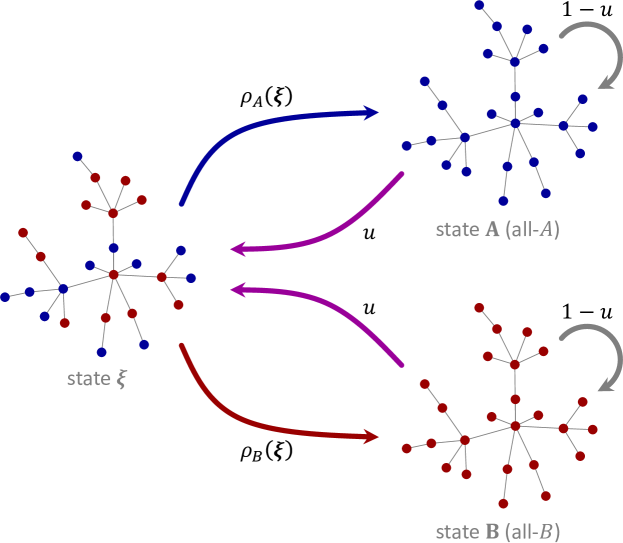
Figure 1: Transitions into a fixed transient state, $\bm{\xi}$, following absorption. When starting from a non-monomorphic state, the process will eventually reach one of the two absorbing states (all-$A$ or all-$B$) by the Fixation Axiom. From each absorbing state, the process transitions to $\bm{\xi}$ with probability $u\geqslant 0$. This “artificial” mutation allows one to focus on the fixation probabilities when the process is started in a fixed initial configuration, $\bm{\xi}$, of $A$ and $B$.

Consider now the Markov chain on the monoallelic states whose transition matrix is

$$\Lambda\coloneqq\bordermatrix{&\mathbf{A}&\mathbf{B}\cr\mathbf{A}&\ \rho_{A}\left(\bm{\xi}\right)&\ \rho_{B}\left(\bm{\xi}\right)\cr\mathbf{B}&\ \rho_{A}\left(\bm{\xi}\right)&\ \rho_{B}\left(\bm{\xi}\right)\cr}.$$ (16)

This chain describes the process in which transitions are first from $\mathbf{A}$ or $\mathbf{B}$ to $\bm{\xi}$, deterministically, and then from $\bm{\xi}$ to $\mathbf{A}$ with probability $\rho_{A}\left(\bm{\xi}\right)$ and to $\mathbf{B}$ with probability $\rho_{B}\left(\bm{\xi}\right)$. This chain is “embedded” in the amended chain in the sense that when $u$ is small, the amended chain spends most of its time in $\left\{\mathbf{A},\mathbf{B}\right\}$, but occasionally it transitions to $\bm{\xi}$ before returning to $\left\{\mathbf{A},\mathbf{B}\right\}$ according to the fixation probabilities. More formally, on a state-by-state basis, the stationary distribution of the embedded chain coincides with $\pi_{\circlearrowright\left(\bm{\xi}\right)}$ on the monoallelic states in the limit $u\rightarrow 0$ (Fudenberg and Imhof, 2006, Theorem 2), i.e.

$$\lim_{u\rightarrow 0}\pi_{\circlearrowright\left(\bm{\xi}\right)}\left(\mathbf{x}\right) =\begin{cases}\displaystyle\rho_{A}\left(\bm{\xi}\right)&\displaystyle\mathbf{x}=\mathbf{A},\\ &\\ &\\ \displaystyle\rho_{B}\left(\bm{\xi}\right)&\displaystyle\mathbf{x}=\mathbf{B},\\ &\\ &\\ \displaystyle 0&\displaystyle\mathbf{x}\not\in\left\{\mathbf{A},\mathbf{B}\right\}.\end{cases}$$ (17)

The following result, which is key to our methodology, shows that sojourn times of the original chain coincide with the $u$-derivative, at $u=0$, of the stationary distribution for the amended chain:

Proposition 1.

For every non-monoallelic state $\mathbf{x}\in\mathbb{B}_{\intercal}^{N}$,

$$\frac{d}{du}\Bigg{|}_{u=0}\pi_{\circlearrowright\left(\bm{\xi}\right)}\left(\mathbf{x}\right) =t_{\bm{\xi}}\left(\mathbf{x}\right).$$ (18)

Proof.

For $\mathbf{x}\in\mathbb{B}_{\intercal}^{N}$, stationarity implies

$$\pi_{\circlearrowright\left(\bm{\xi}\right)}\left(\mathbf{x}\right) =\sum_{\mathbf{y}\in\mathbb{B}^{N}}\pi_{\circlearrowright\left(\bm{\xi}\right)}\left(\mathbf{y}\right)P_{\mathbf{y}\rightarrow\mathbf{x}}^{\circlearrowright\left(\bm{\xi}\right)}$$

$$=\sum_{\mathbf{y}\in\mathbb{B}_{\intercal}^{N}}\pi_{\circlearrowright\left(\bm{\xi}\right)}\left(\mathbf{y}\right)P_{\mathbf{y}\rightarrow\mathbf{x}}+u\delta_{\bm{\xi},\mathbf{x}}\left(\pi_{\circlearrowright\left(\bm{\xi}\right)}\left(\mathbf{A}\right)+\pi_{\circlearrowright\left(\bm{\xi}\right)}\left(\mathbf{B}\right)\right),$$ (19)

where the Kronecker symbol $\delta_{\mathbf{x},\bm{\xi}}$ is equal to 1 if $\mathbf{x}=\bm{\xi}$ and 0 otherwise. Taking the $u$-derivative at $u=0$, and noting that $\lim_{u\rightarrow 0}\left(\pi_{\circlearrowright\left(\bm{\xi}\right)}\left(\mathbf{A}\right)+\pi_{\circlearrowright\left(\bm{\xi}\right)}\left(\mathbf{B}\right)\right)=1$ by Eq. (17), we obtain

$$\frac{d}{du}\Bigg{|}_{u=0}\pi_{\circlearrowright\left(\bm{\xi}\right)}\left(\mathbf{x}\right)=\sum_{\mathbf{y}\in\mathbb{B}_{\intercal}^{N}}\frac{d}{du}\Bigg{|}_{u=0}\pi_{\circlearrowright\left(\bm{\xi}\right)}\left(\mathbf{y}\right)P_{\mathbf{y}\rightarrow\mathbf{x}}+\delta_{\bm{\xi},\mathbf{x}}.$$ (20)

We observe that $\frac{d}{du}\Big{|}_{u=0}\pi_{\circlearrowright\left(\bm{\xi}\right)}\left(\mathbf{x}\right)$ satisfies the same recurrence relation, Eq. (14), as $t_{\bm{\xi}}\left(\mathbf{x}\right)$. Since this recurrence relation uniquely defines the times $t_{\bm{\xi}}\left(\mathbf{x}\right)$, we have Eq. (18). ∎

It follows immediately from Proposition 1 that $t_{\bm{\xi}}\left(\mathbb{B}_{\intercal}^{N}\right)$, the expected time to absorption when starting from state $\bm{\xi}$, is equal to $\lim_{u\rightarrow 0}\pi_{\circlearrowright\left(\bm{\xi}\right)}\left(\mathbb{B}_{\intercal}^{N}\right)/u$. With $\operatorname{\mathbb{E}}_{\circlearrowright\left(\bm{\xi}\right)}\left[\cdot\right]$ denoting expectation with respect to $\pi_{\circlearrowright\left(\bm{\xi}\right)}$, we have the following result:

Corollary 1.

For any function $\varphi:\mathbb{B}^{N}\rightarrow\mathbb{R}$ with $\varphi\left(\mathbf{A}\right)=\varphi\left(\mathbf{B}\right)=0$,

$$\frac{d}{du}\Bigg{|}_{u=0}\operatorname{\mathbb{E}}_{\circlearrowright\left(\bm{\xi}\right)}\left[\varphi\right]=\sum_{t=0}^{\infty}\operatorname{\mathbb{E}}\left[\varphi\left(\mathbf{x}^{t}\right)\mid\mathbf{x}^{0}=\bm{\xi}\right],$$ (21)

and the sum on the right-hand side converges absolutely.

Proof.

$\sum_{t=0}^{\infty}\left|\operatorname{\mathbb{E}}\left[\varphi\left(\mathbf{x}^{t}\right)\mid\mathbf{x}^{0}=\bm{\xi}\right]\right|$ is bounded by $t_{\bm{\xi}}\left(\mathbb{B}_{\intercal}^{N}\right)\max_{\mathbf{x}\in\mathbb{B}_{\intercal}^{N}}\left|\varphi\left(\mathbf{x}\right)\right|$, so the right-hand side of Eq. (21) converges absolutely. We may therefore rearrange this summation to obtain

$$\sum_{t=0}^{\infty}\operatorname{\mathbb{E}}\left[\varphi\left(\mathbf{x}^{t}\right)\mid\mathbf{x}^{0}=\bm{\xi}\right] =\sum_{t=0}^{\infty}\sum_{\mathbf{x}\in\mathbb{B}_{\intercal}^{N}}\operatorname{\mathbb{P}}\left[\mathbf{x}^{t}=\mathbf{x}\mid\mathbf{x}^{0}=\bm{\xi}\right]\varphi\left(\mathbf{x}\right)$$

$$=\sum_{\mathbf{x}\in\mathbb{B}_{\intercal}^{N}}\varphi\left(\mathbf{x}\right)\sum_{t=0}^{\infty}\operatorname{\mathbb{P}}\left[\mathbf{x}^{t}=\mathbf{x}\mid\mathbf{x}^{0}=\bm{\xi}\right]$$

$$=\sum_{\mathbf{x}\in\mathbb{B}_{\intercal}^{N}}\varphi\left(\mathbf{x}\right)t_{\bm{\xi}}\left(\mathbf{x}\right)$$

$$=\frac{d}{du}\Bigg{|}_{u=0}\operatorname{\mathbb{E}}_{\circlearrowright\left(\bm{\xi}\right)}\left[\varphi\right],$$ (22)

as desired. ∎

In light of Corollary 1, we define the operator $\langle\cdot\rangle_{\bm{\xi}}$, acting on state functions $\varphi:\mathbb{B}^{N}\rightarrow\mathbb{R}$ with $\varphi\left(\mathbf{A}\right)=\varphi\left(\mathbf{B}\right)=0$, by

$$\langle\varphi\rangle_{\bm{\xi}} \coloneqq\frac{d}{du}\Bigg{|}_{u=0}\operatorname{\mathbb{E}}_{\circlearrowright\left(\bm{\xi}\right)}\left[\varphi\right]=\sum_{t=0}^{\infty}\operatorname{\mathbb{E}}\left[\varphi(\mathbf{x}^{t})\mid\mathbf{x}^{0}=\bm{\xi}\right].$$ (23)

We will use the notation $\langle\cdot\rangle_{\bm{\xi}}^{\circ}$ to indicate that the above expectations are taken under neutral drift ($\delta=0$).

For any function $\varphi:\mathbb{B}^{N}\rightarrow\mathbb{R}$ and any $\widetilde{\alpha}:\left\{1,\dots,N\right\}\rightarrow\left\{1,\dots,N\right\}$, we define $\varphi_{\widetilde{\alpha}}:\mathbb{B}^{N}\rightarrow\mathbb{R}$ by $\varphi_{\widetilde{\alpha}}\left(\mathbf{x}\right)=\varphi\left(\mathbf{x}_{\widetilde{\alpha}}\right)$. If $\varphi\left(\mathbf{A}\right)=\varphi\left(\mathbf{B}\right)=0$, then

$$\left\langle\varphi\right\rangle_{\bm{\xi}}^{\circ} =\varphi\left(\bm{\xi}\right)+\sum_{t=0}^{\infty}\operatorname{\mathbb{E}}^{\circ}\left[\varphi(\mathbf{x}^{t+1})\mid\mathbf{x}^{0}=\bm{\xi}\right]$$

$$=\varphi\left(\bm{\xi}\right)+\sum_{t=0}^{\infty}\sum_{\left(R,\alpha\right)}p_{\left(R,\alpha\right)}^{\circ}\operatorname{\mathbb{E}}^{\circ}\left[\varphi\left(\mathbf{x}^{t}_{\widetilde{\alpha}}\right)\mid\mathbf{x}^{0}=\bm{\xi}\right]$$

$$=\varphi\left(\bm{\xi}\right)+\sum_{\left(R,\alpha\right)}p_{\left(R,\alpha\right)}^{\circ}\left\langle\varphi_{\widetilde{\alpha}}\right\rangle_{\bm{\xi}}^{\circ},$$ (24)

which gives the following lemma:

Lemma 1.

For any state function $\varphi:\mathbb{B}^{N}\rightarrow\mathbb{R}$ with $\varphi\left(\mathbf{A}\right)=\varphi\left(\mathbf{B}\right)=0$,

$$\left\langle\varphi\right\rangle_{\bm{\xi}}^{\circ} =\varphi\left(\bm{\xi}\right)+\sum_{\left(R,\alpha\right)}p_{\left(R,\alpha\right)}^{\circ}\left\langle\varphi_{\widetilde{\alpha}}\right\rangle_{\bm{\xi}}^{\circ}.$$ (25)

Allen and McAvoy (2019) introduced the rare-mutation conditional (RMC) distribution, defined for a state $\mathbf{x}$ as $\lim_{u\rightarrow 0}\operatorname{\mathbb{P}}_{\circlearrowright\left(\bm{\xi}\right)}\left[\mathbf{X}=\mathbf{x}\mid\mathbf{x}\in\mathbb{B}_{\intercal}^{N}\right]$, where $\operatorname{\mathbb{P}}_{\circlearrowright\left(\bm{\xi}\right)}\left[\cdot\right]$ denotes probability with respect to $\pi_{\circlearrowright\left(\bm{\xi}\right)}$. Here, we show that this distribution can be equated to the fraction of time spent in state $\mathbf{x}$ out of all transient states:

Corollary 2.

For each $\mathbf{x}\in\mathbb{B}_{\intercal}^{N}$

$$\lim_{u\rightarrow 0}\operatorname{\mathbb{P}}_{\circlearrowright\left(\bm{\xi}\right)}\left[\mathbf{X}=\mathbf{x}\mid\mathbf{x}\in\mathbb{B}_{\intercal}^{N}\right]=\frac{t_{\bm{\xi}}\left(\mathbf{x}\right)}{t_{\bm{\xi}}\left(\mathbb{B}_{\intercal}^{N}\right)}.$$ (26)

Proof.

For $\mathbf{x}\in\mathbb{B}_{\intercal}^{N}$,

$$\lim_{u\rightarrow 0}\operatorname{\mathbb{P}}_{\circlearrowright\left(\bm{\xi}\right)}\left[\mathbf{X}=\mathbf{x}\mid\mathbf{x}\in\mathbb{B}_{\intercal}^{N}\right] =\lim_{u\rightarrow 0}\frac{\pi_{\circlearrowright\left(\bm{\xi}\right)}\left(\mathbf{x}\right)}{\pi_{\circlearrowright\left(\bm{\xi}\right)}\left(\mathbb{B}_{\intercal}^{N}\right)}$$

$$=\frac{\lim_{u\rightarrow 0}\pi_{\circlearrowright\left(\bm{\xi}\right)}\left(\mathbf{x}\right)/u}{\lim_{u\rightarrow 0}\pi_{\circlearrowright\left(\bm{\xi}\right)}\left(\mathbb{B}_{\intercal}^{N}\right)/u}$$

$$=\frac{t_{\bm{\xi}}\left(\mathbf{x}\right)}{t_{\bm{\xi}}\left(\mathbb{B}_{\intercal}^{N}\right)},$$ (27)

by Proposition 1. ∎

Finally, we introduce a set-valued Markov chain that will be used in the proof of our main result. The states of this Markov chain are subsets of $\left\{1,\dots,N\right\}$. From a given state $I\subseteq\left\{1,\dots,N\right\}$, a new state $I^{\prime}$ is determined by choosing a replacement event $\left(R,\alpha\right)$ according to the neutral probabilities $p_{\left(R,\alpha\right)}^{\circ}$, and setting $I^{\prime}=\widetilde{\alpha}\left(I\right)$. This Markov chain, which we denote $\mathcal{C}$, can be understood as a coalescent process (Kingman, 1982; Liggett, 1985; Cox, 1989; Wakeley, 2016). At each time-step, $\mathcal{C}$ transitions from a set of individuals $I\subseteq\{1,\ldots,N\}$ to the set $\widetilde{\alpha}\left(I\right)$ of parents of these individuals. (In the case that an individual $i\in I$ is not replaced, the “parent” is $i$ itself; that is, $\widetilde{\alpha}\left(i\right)=i$.) Thus, with $\mathcal{C}_{0}=\left\{1,\dots,N\right\}$, the state of the process after $t$ steps can be understood as the set of ancestors of the current population, at time $t$ before the present.

By the Fixation Axiom, $\mathcal{C}$ has a single closed communicating class consisting only of singleton subsets. (In biological terms, the population’s ancestry eventually converges on a common ancestor. The event that $\mathcal{C}$ first reaches a singleton set is called coalescence, and the vertex in this singleton set represents the location of the population’s most recent common ancestor.) It follows that $\mathcal{C}$ has a unique stationary distribution concentrated on the singleton subsets. In this stationary distribution, the probability of the singleton set $\{i\}$ in this stationary distribution is given by the reproductive value $\pi_{i}$.

4 Fixation probabilities

We now prove our main results regarding fixation probabilities. First, we show that the weak-selection expansion of a trait’s fixation probability has a particular form:

Theorem 1.

For any fixed initial configuration $\bm{\xi}\in\mathbb{B}_{\intercal}^{N}$,

$$\rho_{A}\left(\bm{\xi}\right) =\widehat{\xi}+\delta\left\langle\frac{d}{d\delta}\Bigg{|}_{\delta=0}\widehat{\Delta}_{\mathrm{sel}}\right\rangle_{\bm{\xi}}^{\circ}+O\left(\delta^{2}\right).$$ (28)

Theorem 1 generalizes earlier results of Rousset (2003), Lessard and Ladret (2007), Chen (2013), and Van Cleve (2015).

Proof.

In the chain defined by Eq. (15), the expected change in the reproductive-value-weighted frequency of $A$ in state $\mathbf{x}$, in one step of the process, is given by

$$\widehat{\Delta}_{\circlearrowright\left(\bm{\xi}\right)}\left(\mathbf{x}\right) =\begin{cases}\displaystyle-u\left(1-\widehat{\xi}\right)&\displaystyle\mathbf{x}=\mathbf{A},\\ &\\ \displaystyle u\widehat{\xi}&\displaystyle\mathbf{x}=\mathbf{B},\\ &\\ \displaystyle\widehat{\Delta}_{\mathrm{sel}}\left(\mathbf{x}\right)&\displaystyle\mathbf{x}\not\in\left\{\mathbf{A},\mathbf{B}\right\}.\end{cases}$$ (29)

Averaging this expected change out over the distribution $\pi_{\circlearrowright\left(\bm{\xi}\right)}$ gives

$$0 =\operatorname{\mathbb{E}}_{\circlearrowright\left(\bm{\xi}\right)}\left[\widehat{\Delta}_{\circlearrowright\left(\bm{\xi}\right)}\right]$$

$$=\operatorname{\mathbb{E}}_{\circlearrowright\left(\bm{\xi}\right)}\left[\widehat{\Delta}_{\mathrm{sel}}\right]-u\pi_{\circlearrowright\left(\bm{\xi}\right)}\left(\mathbf{A}\right)\left(1-\widehat{\xi}\right)+u\pi_{\circlearrowright\left(\bm{\xi}\right)}\left(\mathbf{B}\right)\widehat{\xi}.$$ (30)

Differentiating both sides of this equation with respect to $u$ at $u=0$, applying Eq. (17), and rearranging, we obtain

$$\rho_{A}\left(\bm{\xi}\right)=\widehat{\xi}+\left\langle\widehat{\Delta}_{\mathrm{sel}}\right\rangle_{\bm{\xi}}.$$ (31)

Since $\widehat{\Delta}_{\mathrm{sel}}^{\circ}\left(\mathbf{x}\right)=0$ for every $\mathbf{x}\in\mathbb{B}^{N}$, and since the replacement rule is a smooth function of $\delta$ around $0$, we have

$$\left\langle\widehat{\Delta}_{\mathrm{sel}}\right\rangle_{\bm{\xi}} =\delta\frac{d}{d\delta}\Bigg{|}_{\delta=0}\left\langle\widehat{\Delta}_{\mathrm{sel}}\right\rangle_{\bm{\xi}}+O\left(\delta^{2}\right)$$

$$=\delta\left\langle\frac{d}{d\delta}\Bigg{|}_{\delta=0}\widehat{\Delta}_{\mathrm{sel}}\right\rangle_{\bm{\xi}}^{\circ}+O\left(\delta^{2}\right).$$ (32)

The interchange of the $\langle\cdot\rangle_{\bm{\xi}}^{\circ}$ operator with the $\delta$-derivative is justified by Corollary 1. Combining this equation with Eq. (31) completes the proof. ∎

Alternatively, Theorem 1 can be established by writing

$$\rho_{A}\left(\bm{\xi}\right) =\lim_{t\rightarrow\infty}\operatorname{\mathbb{E}}\left[\widehat{x}^{t}\mid\mathbf{x}^{0}=\bm{\xi}\right]$$

$$=\widehat{\xi}+\sum_{t=0}^{\infty}\operatorname{\mathbb{E}}\left[\widehat{x}^{t+1}-\widehat{x}^{t}\mid\mathbf{x}^{0}=\bm{\xi}\right]$$

$$=\widehat{\xi}+\sum_{t=0}^{\infty}\operatorname{\mathbb{E}}\left[\widehat{\Delta}_{\mathrm{sel}}\left(\mathbf{x}^{t}\right)\mid\mathbf{x}^{0}=\bm{\xi}\right]$$

$$=\widehat{\xi}+\left\langle\widehat{\Delta}_{\mathrm{sel}}\right\rangle_{\bm{\xi}}.$$ (33)

This calculation recovers Eq. (31), and the rest of the proof follows as above.

Our second main result provides a systematic way to compute the first-order term of the weak-selection expansion, Eq. (28):

Theorem 2.

For any fixed initial configuration $\bm{\xi}\in\mathbb{B}_{\intercal}^{N}$,

$$\rho_{A}\left(\bm{\xi}\right) =\widehat{\xi}+\delta\left(\sum_{i=1}^{N}\pi_{i}\sum_{j=1}^{N}\sum_{\begin{subarray}{c}I\subseteq\left\{1,\dots,N\right\}\\ 0\leqslant\left|I\right|\leqslant D_{ji}\end{subarray}}c_{I}^{ji}\left(\eta_{\left\{i\right\}\cup I}^{\bm{\xi}}-\eta_{\left\{j\right\}\cup I}^{\bm{\xi}}\right)\right)+O\left(\delta^{2}\right),$$ (34)

where $\eta^{\bm{\xi}}$ is the unique solution to the equations

$$\eta_{I}^{\bm{\xi}} =\widehat{\xi}-\bm{\xi}_{I}+\sum_{\left(R,\alpha\right)}p_{\left(R,\alpha\right)}^{\circ}\eta_{\widetilde{\alpha}\left(I\right)}^{\bm{\xi}}\quad\left(1\leqslant\left|I\right|\leqslant D+1\right);$$ (35a)

$$\sum_{i=1}^{N}\pi_{i}\eta_{\left\{i\right\}}^{\bm{\xi}} =0.$$ (35b)

The term $D$ appearing in this system is the degree of the process under weak selection; see Definition 1. To simplify notation, in what follows we occasionally drop the bracket notation when using $\eta$ (e.g. $\eta_{i}^{\bm{\xi}}$ instead of $\eta_{\left\{i\right\}}^{\bm{\xi}}$).

Proof.

Let us define

$$\eta_{I}^{\bm{\xi}}\coloneqq\left\langle\widehat{x}-\mathbf{x}_{I}\right\rangle_{\bm{\xi}}^{\circ}.$$ (36)

From Theorem 1 and Eqs. (6) and (13), we have

$$\frac{d}{d\delta}\Bigg{|}_{\delta=0}\rho_{A}\left(\bm{\xi}\right) =\left\langle\frac{d}{d\delta}\Bigg{|}_{\delta=0}\widehat{\Delta}_{\mathrm{sel}}\right\rangle_{\bm{\xi}}^{\circ}$$

$$=\sum_{i=1}^{N}\pi_{i}\sum_{j=1}^{N}\sum_{\begin{subarray}{c}I\subseteq\left\{1,\dots,N\right\}\\ 0\leqslant\left|I\right|\leqslant D_{ji}\end{subarray}}c_{I}^{ji}\left\langle\left(x_{j}-x_{i}\right)\mathbf{x}_{I}\right\rangle_{\bm{\xi}}^{\circ}$$

$$=\sum_{i=1}^{N}\pi_{i}\sum_{j=1}^{N}\sum_{\begin{subarray}{c}I\subseteq\left\{1,\dots,N\right\}\\ 0\leqslant\left|I\right|\leqslant D_{ji}\end{subarray}}c_{I}^{ji}\left(\eta_{\left\{i\right\}\cup I}^{\bm{\xi}}-\eta_{\left\{j\right\}\cup I}^{\bm{\xi}}\right),$$ (37)

which proves Eq. (34). Eq. (35b) follows immediately from the definition of $\eta_{I}$ in Eq. (36). To obtain Eq. (35a) we apply Lemma 1:

$$\eta_{I}^{\bm{\xi}} =\left\langle\widehat{x}-\mathbf{x}_{I}\right\rangle_{\bm{\xi}}^{\circ}$$

$$=\widehat{\xi}-\bm{\xi}_{I}+\sum_{\left(R,\alpha\right)}p_{\left(R,\alpha\right)}^{\circ}\left\langle\widehat{x_{\widetilde{\alpha}}}-\mathbf{x}_{\widetilde{\alpha}\left(I\right)}\right\rangle_{\bm{\xi}}^{\circ}$$

$$=\widehat{\xi}-\bm{\xi}_{I}+\sum_{\left(R,\alpha\right)}p_{\left(R,\alpha\right)}^{\circ}\left\langle\widehat{x}-\mathbf{x}_{\widetilde{\alpha}\left(I\right)}\right\rangle_{\bm{\xi}}^{\circ}$$

$$=\widehat{\xi}-\bm{\xi}_{I}+\sum_{\left(R,\alpha\right)}p_{\left(R,\alpha\right)}^{\circ}\eta_{\widetilde{\alpha}\left(I\right)}^{\bm{\xi}},$$ (38)

where the penultimate line follows from the fact that $\widehat{x}$ is a martingale under neutral drift (Allen and McAvoy, 2019, Theorem $7$).

To prove uniqueness of the solution to Eq. (35), we consider the coalescent Markov chain $\mathcal{C}$ defined in the previous section. Let $\mathbf{C}$ be the transition matrix for $\mathcal{C}$, and let $\mathbf{p}$ be its stationary distribution in vector form, which satisfies $\mathbf{p}\left(I\right)=\pi_{i}$ if $I=\left\{i\right\}$ and $\mathbf{p}\left(I\right)=0$ if $\left|I\right|\neq 1$. By uniqueness of the stationary distribution, $\mathbf{C}$ has a simple unit eigenvalue, with corresponding one-dimensional left and right eigenspaces spanned by $\mathbf{p}^{T}$ and $\mathbf{1}$, respectively. We observe that Eq. (35a) can be written in the form $\left(\mathbf{I}-\mathbf{C}\right)\mathbf{y}=\mathbf{b}$, where $\mathbf{y}$ has entries $\eta_{I}^{\bm{\xi}}$ and $\mathbf{b}$ has entries $\widehat{\xi}-\bm{\xi}_{I}$. We have already exhibited a solution for $\mathbf{y}$ in Eq. (36); call this solution $\mathbf{y}_{0}$. By the above remarks about $\mathbf{C}$, the most general solution is $\mathbf{y}=\mathbf{y}_{0}+K\mathbf{1}$ for an arbitrary scalar $K$. Now we impose Eq. (35b), which can be written $\mathbf{p}^{T}\mathbf{y}=0$. Since $\mathbf{p}^{T}\mathbf{y}_{0}=0$ and $\mathbf{p}^{T}\mathbf{1}=1$, we must have $K=0$, which leaves $\mathbf{y}=\mathbf{y}_{0}$ as the unique solution. ∎

Remark 1.

For a process of degree $D$, calculating $\frac{d}{d\delta}\Big{|}_{\delta=0}\rho_{A}$ involves solving a linear system of size $O\left(N^{D+1}\right)$ (Eq. (35)). The complexity of solving for $\pi_{i}$ and $c_{I}^{ij}$ is negligible in comparison. Since the complexity of solving a linear system of $n$ equations is $O\left(n^{3}\right)$, it follows that calculating $\frac{d}{d\delta}\Big{|}_{\delta=0}\rho_{A}$ is $O\left(N^{3\left(D+1\right)}\right)$.

Since the quantities $\eta_{I}$ arise as the solution to a system of equations related to the coalescent Markov chain $\mathcal{C}$, it is natural to ask whether the $\eta_{I}$ have a coalescent-theoretic interpretation. We show in the following sections that, in some cases when the initial state is chosen from a particular probability distribution, the $\eta_{I}$ have a natural interpretation as coalescence times or as branch lengths of a coalescent tree. However, these interpretations do not appear to extend to the case of fixation from an arbitrary initial state $\bm{\xi}$.

5 Stochastic mutant appearance

Having obtained (in Theorems 1 and 2) a weak-selection expansion for fixation probabilities from a particular state $\bm{\xi}$, we now generalize to the case that the initial state is sampled from a probability distribution. Specifically, we introduce the probability measures $\mu_{A}$ and $\mu_{B}$, on $\mathbb{B}_{\intercal}^{N}$, to describe the state of the process after type $A$ or $B$, respectively, has been introduced into the population. We refer to $\mu_{A}$ and $\mu_{B}$ as mutant-appearance distributions, although the initial state could just as well arise by some mechanism other than mutation (migration, experimental manipulation, etc.). These distributions can depend on the intensity of selection, $\delta$, and we assume that they are differentiable at $\delta=0$.

Two mutant-appearance distributions often considered in evolutionary models are uniform initialization (a single mutant appears at a uniformly chosen site; Lieberman et al., 2005; Adlam et al., 2015) and temperature initialization (a single mutant appears at a site chosen proportionally to the death rate $d_{i}$; Allen et al., 2015; Adlam et al., 2015). To define these formally, we define the complement $\overline{\mathbf{x}}$ of a state $\mathbf{x}\in\mathbb{B}^{N}$ by $\overline{x}_{i}\coloneqq 1-x_{i}$ for $i=1,\dots,N$.

Example 1 (Uniform initialization).

$$\mu_{A}\left(\mathbf{1}_{i}\right) =\mu_{B}\left(\overline{\mathbf{1}}_{i}\right)=\frac{1}{N}\quad\left(1\leqslant i\leqslant N\right).$$ (39)

Example 2 (Temperature initialization).

$$\mu_{A}\left(\mathbf{1}_{i}\right) =\frac{d_{i}\left(\mathbf{B}\right)}{\sum_{j=1}^{N}d_{j}\left(\mathbf{B}\right)}\quad\left(1\leqslant i\leqslant N\right);$$ (40a)

$$\mu_{B}\left(\overline{\mathbf{1}}_{i}\right) =\frac{d_{i}\left(\mathbf{A}\right)}{\sum_{j=1}^{N}d_{j}\left(\mathbf{A}\right)}\quad\left(1\leqslant i\leqslant N\right).$$ (40b)

Unlike uniform initialization, temperature initialization opens up the possibility that the mutant-appearance distributions depend on the intensity of selection, $\delta$.

We call a mutant-appearance distribution symmetric if it does not distinguish between the two types:

Definition 2.

We say that $\mu_{A}$ and $\mu_{B}$ are symmetric if $\mu_{A}\left(\overline{\bm{\xi}}\right)=\mu_{B}\left(\bm{\xi}\right)$ for every $\bm{\xi}\in\mathbb{B}_{\intercal}^{N}$.

Uniform initialization (Example 1) gives symmetric $\mu_{A}$ and $\mu_{B}$ by definition. If mutant initialization is temperature-based (Example 2), then $\mu_{A}$ and $\mu_{B}$ are symmetric when $d_{i}\left(\mathbf{A}\right)=d_{i}\left(\mathbf{B}\right)$ for $i=1,\dots,N$. This condition is obviously satisfied under neutral drift ($\delta=0$) but could be violated when $\delta>0$.

The expected fixation probabilities for $A$ and $B$, initialized according to $\mu_{A}$ and $\mu_{B}$, respectively, are

$$\operatorname{\mathbb{E}}_{\mu_{A}}\left[\rho_{A}\right] =\sum_{\bm{\xi}\in\mathbb{B}_{\intercal}^{N}}\mu_{A}\left(\bm{\xi}\right)\rho_{A}\left(\bm{\xi}\right);$$ (41a)

$$\operatorname{\mathbb{E}}_{\mu_{B}}\left[\rho_{B}\right] =\sum_{\bm{\xi}^{\prime}\in\mathbb{B}_{\intercal}^{N}}\mu_{B}\left(\bm{\xi}^{\prime}\right)\rho_{B}\left(\bm{\xi}^{\prime}\right).$$ (41b)

Since $\rho_{A}^{\circ}\left(\bm{\xi}\right)=\widehat{\xi}$ and $\rho_{B}^{\circ}\left(\bm{\xi}\right)=1-\widehat{\xi}$ when $\delta=0$, we have $\operatorname{\mathbb{E}}_{\mu_{A}}^{\circ}\left[\rho_{A}^{\circ}\right]=\operatorname{\mathbb{E}}_{\mu_{A}}^{\circ}\left[\widehat{\xi}\right]$ and $\operatorname{\mathbb{E}}_{\mu_{B}}^{\circ}\left[\rho_{B}^{\circ}\right]=1-\operatorname{\mathbb{E}}_{\mu_{B}}^{\circ}\left[\widehat{\xi}\right]$. More generally, we have $\operatorname{\mathbb{E}}_{\mu_{B}}\left[\rho_{B}\right]=1-\operatorname{\mathbb{E}}_{\mu_{B}}\left[\rho_{A}\right]$.

As an immediate consequence of Theorem 2, we obtain the following result for the fixation probability of a given type from a given mutant appearance distribution:

Corollary 3.

If $\mu_{A}$ is a mutant-appearance distribution for $A$, then

$$\frac{d}{d\delta}\Bigg{|}_{\delta=0}\operatorname{\mathbb{E}}_{\mu_{A}}\left[\rho_{A}\right] =\frac{d}{d\delta}\Bigg{|}_{\delta=0}\operatorname{\mathbb{E}}_{\mu_{A}}\left[\widehat{\xi}\right]+\sum_{i=1}^{N}\pi_{i}\sum_{j=1}^{N}\sum_{\begin{subarray}{c}I\subseteq\left\{1,\dots,N\right\}\\ 0\leqslant\left|I\right|\leqslant D_{ji}\end{subarray}}c_{I}^{ji}\left(\eta_{\left\{i\right\}\cup I}^{\mu_{A}}-\eta_{\left\{j\right\}\cup I}^{\mu_{A}}\right),$$ (42)

where $\eta^{\mu_{A}}$ is the unique solution to the equations

$$\eta_{I}^{\mu_{A}} =\operatorname{\mathbb{E}}_{\mu_{A}}^{\circ}\left[\widehat{\xi}-\bm{\xi}_{I}\right]+\sum_{\left(R,\alpha\right)}p_{\left(R,\alpha\right)}^{\circ}\eta_{\widetilde{\alpha}\left(I\right)}^{\mu_{A}}\quad\left(1\leqslant\left|I\right|\leqslant D+1\right);$$ (43a)

$$\sum_{i=1}^{N}\pi_{i}\eta_{i}^{\mu_{A}} =0.$$ (43b)

Similarly, since $\frac{d}{d\delta}\Big{|}_{\delta=0}\operatorname{\mathbb{E}}_{\mu_{B}}\left[\rho_{B}\right]=-\frac{d}{d\delta}\Big{|}_{\delta=0}\operatorname{\mathbb{E}}_{\mu_{B}}\left[\rho_{A}\right]$, we have

$$\frac{d}{d\delta}\Bigg{|}_{\delta=0}\operatorname{\mathbb{E}}_{\mu_{B}}\left[\rho_{B}\right] =-\frac{d}{d\delta}\Bigg{|}_{\delta=0}\operatorname{\mathbb{E}}_{\mu_{B}}\left[\widehat{\xi}\right]-\sum_{i=1}^{N}\pi_{i}\sum_{j=1}^{N}\sum_{\begin{subarray}{c}I\subseteq\left\{1,\dots,N\right\}\\ 0\leqslant\left|I\right|\leqslant D_{ji}\end{subarray}}c_{I}^{ji}\left(\eta_{\left\{i\right\}\cup I}^{\mu_{B}}-\eta_{\left\{j\right\}\cup I}^{\mu_{B}}\right),$$ (44)

where $\eta^{\mu_{B}}$ is the unique solution to the equations

$$\eta_{I}^{\mu_{B}} =\operatorname{\mathbb{E}}_{\mu_{B}}^{\circ}\left[\widehat{\xi}-\bm{\xi}_{I}\right]+\sum_{\left(R,\alpha\right)}p_{\left(R,\alpha\right)}^{\circ}\eta_{\widetilde{\alpha}\left(I\right)}^{\mu_{B}}\quad\left(1\leqslant\left|I\right|\leqslant D+1\right);$$ (45a)

$$\sum_{i=1}^{N}\pi_{i}\eta_{i}^{\mu_{B}} =0.$$ (45b)

In the case of uniform initialization (Example 1), we have $\operatorname{\mathbb{E}}_{\mu_{A}}\left[\xi_{i}\right]=1/N$ for all $i\in\left\{1,\dots,N\right\}$. In particular, $\operatorname{\mathbb{E}}_{\mu_{A}}^{\circ}\left[\widehat{\xi}-\xi_{i}\right]=0$ for every $i$. Since $\eta^{\mu_{A}}_{i}=0$ for $i=1,\dots,N$ is then a solution to Eq. (43a), and since this solution satisfies Eq. (43b), it must be the unique solution to Eq. (43) in the case that $\left|I\right|=1$ (see the proof of Theorem 2). (This argument is used repeatedly in later examples.) Furthermore, $\operatorname{\mathbb{E}}_{\mu_{A}}\left[\bm{\xi}_{I}\right]=0$ for all $\left|I\right|\geqslant 2$. Eq. (43) then simplifies to

$$\eta^{\mu_{A}}_{I}=\begin{cases}\displaystyle\frac{1}{N}+\sum_{\left(R,\alpha\right)}p_{\left(R,\alpha\right)}^{\circ}\eta^{\mu_{A}}_{\widetilde{\alpha}\left(I\right)}&\displaystyle 2\leqslant\left|I\right|\leqslant D+1,\\ &\\ \displaystyle 0&\displaystyle\left|I\right|=1.\end{cases}$$ (46)

In this case, $\eta^{\mu_{A}}_{I}$ is equal to $1/N$ times the expected number of steps for the coalescent Markov chain $\mathcal{C}$ to reach a singleton set from initial set $I$. In biological terms, $N\eta^{\mu_{A}}_{I}$ is the expected time for the lineages of the individuals in set $I$ to coalesce at a most recent common ancestor.

The overall weak-selection expansion of a trait’s fixation probability, in the case of uniform initialization, becomes

$$\operatorname{\mathbb{E}}_{\mu_{A}}\left[\rho_{A}\right]=\frac{1}{N}+\delta\sum_{i=1}^{N}\pi_{i}\sum_{j=1}^{N}\sum_{\begin{subarray}{c}I\subseteq\left\{1,\dots,N\right\}\\ 0\leqslant\left|I\right|\leqslant D_{ji}\end{subarray}}c_{I}^{ji}\left(\eta_{\left\{i\right\}\cup I}^{\mu_{A}}-\eta_{\left\{j\right\}\cup I}^{\mu_{A}}\right)+O\left(\delta^{2}\right).$$ (47)

6 Comparing fixation probabilities

When evaluating which of two competing types is favored by selection, it is common to compare their fixation probabilities. Specifically, the success of $A$ relative to $B$ is often quantified by whether $\operatorname{\mathbb{E}}_{\mu_{A}}\left[\rho_{A}\right]>\operatorname{\mathbb{E}}_{\mu_{B}}\left[\rho_{B}\right]$ ($A$ is favored) or $\operatorname{\mathbb{E}}_{\mu_{A}}\left[\rho_{A}\right]<\operatorname{\mathbb{E}}_{\mu_{B}}\left[\rho_{B}\right]$ ($B$ is favored) (Nowak et al., 2004; Allen and Tarnita, 2014; Tarnita and Taylor, 2014). This comparison is natural when the mutant-appearance distributions, $\mu_{A}$ and $\mu_{B}$, are symmetric.

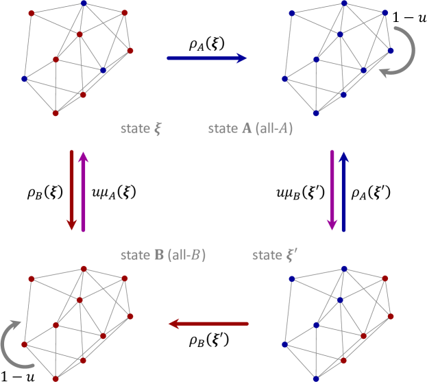
Figure 2: Mutant appearance and fixation in a structured population. In the all-$B$ state, mutants of type $A$ appear based on the mutant-appearance distribution $\mu_{A}$. In the all-$A$ state, mutants of type $B$ appear based on $\mu_{B}$. Once the process transitions into a non-monomorphic state, it will eventually reach one of the two monomorphic states.

When $\mu_{A}$ and $\mu_{B}$ are not symmetric, however, it is less natural to compare $\operatorname{\mathbb{E}}_{\mu_{A}}\left[\rho_{A}\right]$ to $\operatorname{\mathbb{E}}_{\mu_{B}}\left[\rho_{B}\right]$ directly. We therefore derive an alternative measure of success for the asymmetric case. As in Section 3, we find it helpful to work with an amended Markov chain that possesses a unique stationary distribution. To this end, we suppose that, from the monomorphic state $\mathbf{B}$, with probability $u$ the next state is chosen from the distribution $\mu_{A}$; otherwise, with probability $1-u$, the state stays $\mathbf{B}$. Similarly, from the monomorphic state $\mathbf{A}$, with probability $u$ the next state is chosen from the distribution $\mu_{B}$; otherwise, with probability $1-u$, the state stays $\mathbf{B}$. The structure of this amended Markov chain is depicted in Fig. 2. Provided $u>0$, this process has a unique stationary distribution. In analogy to our analysis of mutations into a fixed state in Section 3, we denote this stationary distribution by $\pi_{\circlearrowright\left(\mu_{A},\mu_{B}\right)}$.

We now turn to the limit of low mutation. Applying standard results on stationary distributions in this limit (Fudenberg and Imhof, 2006, Theorem 2), we have

$$\lim_{u\rightarrow 0}\pi_{\circlearrowright\left(\mu_{A},\mu_{B}\right)}\left(\mathbf{x}\right)=\begin{cases}\displaystyle\frac{\operatorname{\mathbb{E}}_{\mu_{A}}\left[\rho_{A}\right]}{\operatorname{\mathbb{E}}_{\mu_{A}}\left[\rho_{A}\right]+\operatorname{\mathbb{E}}_{\mu_{B}}\left[\rho_{B}\right]}&\mathbf{x}=\mathbf{A},\\ &\\ \displaystyle\frac{\operatorname{\mathbb{E}}_{\mu_{B}}\left[\rho_{B}\right]}{\operatorname{\mathbb{E}}_{\mu_{A}}\left[\rho_{A}\right]+\operatorname{\mathbb{E}}_{\mu_{B}}\left[\rho_{B}\right]}&\mathbf{x}=\mathbf{B},\\ &\\ \displaystyle 0&\text{otherwise}.\end{cases}$$ (48)

Intuitively, for small but positive mutation rates, the process is almost always in state $\mathbf{A}$ or $\mathbf{B}$, with the fraction of time spent in $\mathbf{A}$ converging to $\operatorname{\mathbb{E}}_{\mu_{A}}\left[\rho_{A}\right]/\left(\operatorname{\mathbb{E}}_{\mu_{A}}\left[\rho_{A}\right]+\operatorname{\mathbb{E}}_{\mu_{B}}\left[\rho_{B}\right]\right)$.

We say that weak selection favors $A$ over $B$ if the fraction of time spent in state $A$ is greater under weak selection than it is in the neutral case:

Definition 3.

Weak selection favors $A$ over $B$ if

$$\frac{\operatorname{\mathbb{E}}_{\mu_{A}}\left[\rho_{A}\right]}{\operatorname{\mathbb{E}}_{\mu_{A}}\left[\rho_{A}\right]+\operatorname{\mathbb{E}}_{\mu_{B}}\left[\rho_{B}\right]} >\frac{\operatorname{\mathbb{E}}_{\mu_{A}}^{\circ}\left[\rho_{A}^{\circ}\right]}{\operatorname{\mathbb{E}}_{\mu_{A}}^{\circ}\left[\rho_{A}^{\circ}\right]+\operatorname{\mathbb{E}}_{\mu_{B}}^{\circ}\left[\rho_{B}^{\circ}\right]}$$ (49)

(or, equivalently, $\operatorname{\mathbb{E}}_{\mu_{A}}\left[\rho_{A}\right]/\operatorname{\mathbb{E}}_{\mu_{B}}\left[\rho_{B}\right]>\operatorname{\mathbb{E}}_{\mu_{A}}^{\circ}\left[\rho_{A}^{\circ}\right]/\operatorname{\mathbb{E}}_{\mu_{B}}^{\circ}\left[\rho_{B}^{\circ}\right]$) for all sufficiently small $\delta>0$.

When $\mu_{A}^{\circ}$ and $\mu_{B}^{\circ}$ are symmetric (e.g. temperature or uniform initialization), we have $\operatorname{\mathbb{E}}_{\mu_{A}}^{\circ}\left[\rho_{A}^{\circ}\right]=\operatorname{\mathbb{E}}_{\mu_{B}}^{\circ}\left[\rho_{B}^{\circ}\right]$, and weak selection favors $A$ relative to $B$ if and only if $\operatorname{\mathbb{E}}_{\mu_{A}}\left[\rho_{A}\right]>\operatorname{\mathbb{E}}_{\mu_{B}}\left[\rho_{B}\right]$ for all sufficiently small $\delta>0$. For general mutant-appearance distributions, $\mu_{A}$ and $\mu_{B}$, weak selection favors $A$ if

$$\frac{d}{d\delta}\Bigg{|}_{\delta=0}\frac{\operatorname{\mathbb{E}}_{\mu_{A}}\left[\rho_{A}\right]}{\operatorname{\mathbb{E}}_{\mu_{A}}\left[\rho_{A}\right]+\operatorname{\mathbb{E}}_{\mu_{B}}\left[\rho_{B}\right]}>0.$$ (50)

The left-hand side above has the sign of

$$\operatorname{\mathbb{E}}_{\mu_{B}}^{\circ}\left[\rho_{B}^{\circ}\right]\frac{d}{d\delta}\Bigg{|}_{\delta=0}\operatorname{\mathbb{E}}_{\mu_{A}}\left[\rho_{A}\right]-\operatorname{\mathbb{E}}_{\mu_{A}}^{\circ}\left[\rho_{A}^{\circ}\right]\frac{d}{d\delta}\Bigg{|}_{\delta=0}\operatorname{\mathbb{E}}_{\mu_{B}}\left[\rho_{B}\right].$$ (51)

Applying Corollary 3, we obtain the condition

$$\operatorname{\mathbb{E}}_{\mu_{B}}^{\circ}\left[\rho_{B}^{\circ}\right]\frac{d}{d\delta}\Bigg{|}_{\delta=0}\operatorname{\mathbb{E}}_{\mu_{A}}\left[\widehat{\xi}\right]+\operatorname{\mathbb{E}}_{\mu_{A}}^{\circ}\left[\rho_{A}^{\circ}\right]\frac{d}{d\delta}\Bigg{|}_{\delta=0}\operatorname{\mathbb{E}}_{\mu_{B}}\left[\widehat{\xi}\right]$$

$$+\sum_{i=1}^{N}\pi_{i}\sum_{j=1}^{N}\sum_{\begin{subarray}{c}I\subseteq\left\{1,\dots,N\right\}\\ 0\leqslant\left|I\right|\leqslant D_{ji}\end{subarray}}c_{I}^{ji}\left(\eta_{\left\{i\right\}\cup I}^{\mu_{AB}}-\eta_{\left\{j\right\}\cup I}^{\mu_{AB}}\right)>0,$$ (52)

where $\eta_{I}^{\mu_{AB}}\coloneqq\operatorname{\mathbb{E}}_{\mu_{B}}^{\circ}\left[\rho_{B}^{\circ}\right]\eta_{I}^{\mu_{A}}+\operatorname{\mathbb{E}}_{\mu_{A}}^{\circ}\left[\rho_{A}^{\circ}\right]\eta_{I}^{\mu_{B}}$ satisfies the system of equations

$$\eta_{I}^{\mu_{AB}} =\operatorname{\mathbb{E}}_{\mu_{A}}^{\circ}\left[\rho_{A}^{\circ}\right]\left(1-\operatorname{\mathbb{E}}_{\mu_{B}}^{\circ}\left[\bm{\xi}_{I}\right]\right)-\operatorname{\mathbb{E}}_{\mu_{B}}^{\circ}\left[\rho_{B}^{\circ}\right]\operatorname{\mathbb{E}}_{\mu_{A}}^{\circ}\left[\bm{\xi}_{I}\right]$$

$$\quad+\sum_{\left(R,\alpha\right)}p_{\left(R,\alpha\right)}^{\circ}\eta_{\widetilde{\alpha}\left(I\right)}^{\mu_{AB}}\quad\left(1\leqslant\left|I\right|\leqslant D+1\right);$$ (53a)

$$\sum_{i=1}^{N}\pi_{i}\eta_{i}^{\mu_{AB}} =0.$$ (53b)

Eq. (53a) is due to the facts that $\operatorname{\mathbb{E}}_{\mu_{A}}^{\circ}\left[\rho_{A}^{\circ}\right]=\operatorname{\mathbb{E}}_{\mu_{A}}^{\circ}\left[\widehat{\xi}\right]$ and $\operatorname{\mathbb{E}}_{\mu_{B}}^{\circ}\left[\rho_{B}^{\circ}\right]=1-\operatorname{\mathbb{E}}_{\mu_{B}}^{\circ}\left[\widehat{\xi}\right]$.

Example 3.

Consider the case of fixation from a single mutant. Suppose that the initial mutant is located at site $i$ with probability $\mu_{i}$ in both monomorphic states $\mathbf{A}$ and $\mathbf{B}$. That is,

$$\mu_{A}\left(\mathbf{1}_{i}\right)=\mu_{B}\left(\overline{\mathbf{1}}_{i}\right)=\mu_{i}\quad\left(1\leqslant i\leqslant N\right).$$ (54)

All states not of the form $\mathbf{1}_{i}$ for $i\in\{1,\ldots,N\}$ have probability zero in $\mu_{A}$, and states not of the form $\overline{\mathbf{1}}_{i}$ have probability zero in $\mu_{B}$. Then we have $\operatorname{\mathbb{E}}_{\mu_{A}}^{\circ}\left[\xi_{i}\right]=\mu_{i}$ and $\operatorname{\mathbb{E}}_{\mu_{B}}^{\circ}\left[\xi_{i}\right]=1-\mu_{i}$. For non-singleton $I$, we have $\operatorname{\mathbb{E}}_{\mu_{A}}^{\circ}\left[\bm{\xi}_{I}\right]=0$ and $\operatorname{\mathbb{E}}_{\mu_{B}}^{\circ}\left[\bm{\xi}_{I}\right]=1-\sum_{i\in I}\mu_{i}$. We also have $\operatorname{\mathbb{E}}_{\mu_{A}}^{\circ}\left[\rho_{A}^{\circ}\right]=\operatorname{\mathbb{E}}_{\mu_{B}}^{\circ}\left[\rho_{B}^{\circ}\right]$ by symmetry, and both $\operatorname{\mathbb{E}}_{\mu_{A}}\left[\widehat{\xi}\right]$ and $\operatorname{\mathbb{E}}_{\mu_{B}}\left[\widehat{\xi}\right]$ are independent of $\delta$. In this case, weak selection favors $A$ if

$$\sum_{i=1}^{N}\pi_{i}\sum_{j=1}^{N}\sum_{\begin{subarray}{c}I\subseteq\left\{1,\dots,N\right\}\\ 1\leqslant\left|I\right|\leqslant D_{ji}\end{subarray}}c_{I}^{ji}\left(\eta_{\left\{i\right\}\cup I}^{\mu_{AB}}-\eta_{\left\{j\right\}\cup I}^{\mu_{AB}}\right)>0,$$ (55)

where the $\eta_{I}^{\mu_{AB}}$ (upon rescaling by $1/\operatorname{\mathbb{E}}_{\mu_{A}}^{\circ}\left[\rho_{A}^{\circ}\right]$) satisfy the simplified recurrence relation

$$\eta_{I}^{\mu_{AB}}=\begin{cases}\displaystyle\sum_{i\in I}\mu_{i}+\sum_{\left(R,\alpha\right)}p_{\left(R,\alpha\right)}^{\circ}\eta_{\widetilde{\alpha}\left(I\right)}^{\mu_{AB}}&\displaystyle 2\leqslant\left|I\right|\leqslant D+1,\\ &\\ \displaystyle 0&\displaystyle\left|I\right|=1.\end{cases}$$ (56)

7 Application to constant fecundity

Constant (or frequency-independent) fecundity refers to the case in which the fecundity (reproductive rate) of an individual depends on only its type and not on the composition of the rest of the population. A common setup has a mutant ($A$) of reproductive rate $r>0$ competing against a resident ($B$) of reproductive rate 1 (Lieberman et al., 2005; Broom and Rychtář, 2008; Broom et al., 2011; Voorhees, 2013; Monk et al., 2014; Hindersin and Traulsen, 2015; Kaveh et al., 2015; Cuesta et al., 2017; Pavlogiannis et al., 2018; Möller et al., 2019; Tkadlec et al., 2019). The fixation probability of the mutant type is then a function of $r$, which we can write as $\rho_{A}\left(r;\bm{\xi}\right)$, where $\bm{\xi}\in\mathbb{B}_{\intercal}^{N}$ is the initial configuration of the mutant and resident.

A common feature of these models is that the fecundity is interpreted in a relative sense, meaning that $r$ quantifies the reproductive rate of $A$ relative to $B$. Consequently, the fixation probabilities of both types are invariant under rescaling the reproductive rates of all individuals. In particular, the fixation probability of a mutant of reproductive rate $r$ competing against a resident of reproductive rate 1 is equal (upon dividing by $r$) to the fixation probability of a mutant of reproductive rate 1 competing against a resident of reproductive rate $r^{-1}$. By interchanging the roles of $A$ and $B$, we see that fixation probabilities satisfy the duality

$$\rho_{A}\left(r;\bm{\xi}\right) =1-\rho_{A}\left(r^{-1};\overline{\bm{\xi}}\right).$$ (57)

For $r$ close to 1, meaning that the mutation has only a small effect on fecundity, a trait’s fixation probability can be analyzed using weak-selection methods such as those considered here (Allen et al., 2020). To apply these methods, we define the mutant’s selection coefficient as $s=r-1$. We then obtain an expansion of the fixation probability, $\rho_{A}\left(1+s;\bm{\xi}\right)$, around $s=0$. The selection coefficient $s$ plays a similar role to the selection intensity $\delta$ in the foregoing sections, except that $s$ can also be negative, indicating a disadvantageous mutant.

Taking the $s$-derivative of both sides of Eq. (57) at $s=0$, it follows that

$$\frac{d}{ds}\Bigg{|}_{s=0}\rho_{A}\left(1+s;\bm{\xi}\right) =\frac{d}{ds}\Bigg{|}_{s=0}\rho_{A}\left(1+s;\overline{\bm{\xi}}\right)$$

$$=\frac{1}{2}\frac{d}{ds}\Bigg{|}_{s=0}\left(\rho_{A}\left(1+s;\bm{\xi}\right)+\rho_{A}\left(1+s;\overline{\bm{\xi}}\right)\right).$$ (58)

Applying Theorem 2 (with $s$ in place of $\delta$), we have the following weak-selection expansion for $\rho_{A}$:

$$\rho_{A}\left(1+s;\bm{\xi}\right) =\widehat{\xi}+\frac{s}{2}\sum_{i=1}^{N}\pi_{i}\sum_{j=1}^{N}\sum_{\begin{subarray}{c}I\subseteq\left\{1,\dots,N\right\}\\ 0\leqslant\left|I\right|\leqslant D_{ji}\end{subarray}}c_{I}^{ji}\left(\widetilde{\eta}_{\left\{i\right\}\cup I}^{\bm{\xi}}-\widetilde{\eta}_{\left\{j\right\}\cup I}^{\bm{\xi}}\right)+O\left(s^{2}\right),$$ (59)

where $\widetilde{\eta}_{I}^{\bm{\xi}}\coloneqq\eta_{I}^{\bm{\xi}}+\eta_{I}^{\overline{\bm{\xi}}}$. These $\widetilde{\eta}_{I}^{\bm{\xi}}$ are the unique solution to the recurrence relation

$$\widetilde{\eta}_{I}^{\bm{\xi}}=\begin{cases}\displaystyle 1-\left(\bm{\xi}_{I}+\overline{\bm{\xi}}_{I}\right)+\sum_{\left(R,\alpha\right)}p_{\left(R,\alpha\right)}^{\circ}\widetilde{\eta}_{\widetilde{\alpha}\left(I\right)}^{\bm{\xi}}&\displaystyle 2\leqslant\left|I\right|\leqslant D+1,\\ &\\ \displaystyle 0&\displaystyle\left|I\right|=1.\end{cases}$$ (60)

Note that $\bm{\xi}_{I}+\overline{\bm{\xi}}_{I}$ is equal to 1 if all individuals in $I$ have the same type in $\bm{\xi}$ (i.e. $\xi_{i}=\xi_{j}$ for all $i,j\in I$) and 0 otherwise. In particular, $\xi_{i}+\overline{\xi}_{i}=1$ for all $i=1,\dots,N$, which is why $\widetilde{\eta}_{I}^{\bm{\xi}}=0$ for $|I|=1$.

If the initial state $\bm{\xi}$ is drawn from a mutant-appearance distribution, $\mu_{A}$, we then have

$$\frac{d}{ds}\Bigg{|}_{s=0}\operatorname{\mathbb{E}}_{\mu_{A}}\left[\rho_{A}\right] =\frac{d}{ds}\Bigg{|}_{s=0}\operatorname{\mathbb{E}}_{\mu_{A}}\left[\widehat{\xi}\right]+\frac{1}{2}\sum_{i=1}^{N}\pi_{i}\sum_{j=1}^{N}\sum_{\begin{subarray}{c}I\subseteq\left\{1,\dots,N\right\}\\ 0\leqslant\left|I\right|\leqslant D_{ji}\end{subarray}}c_{I}^{ji}\left(\widetilde{\eta}_{\left\{i\right\}\cup I}^{\mu_{A}}-\widetilde{\eta}_{\left\{j\right\}\cup I}^{\mu_{A}}\right),$$ (61)

where

$$\widetilde{\eta}^{\mu_{A}}_{I} =\begin{cases}\displaystyle 1-\operatorname{\mathbb{E}}_{\mu_{A}}^{\circ}\left[\bm{\xi}_{I}+\overline{\bm{\xi}}_{I}\right]+\sum_{\left(R,\alpha\right)}p_{\left(R,\alpha\right)}^{\circ}\widetilde{\eta}_{\widetilde{\alpha}\left(I\right)}^{\mu_{A}}&\displaystyle 2\leqslant\left|I\right|\leqslant D+1,\\ &\\ \displaystyle 0&\displaystyle\left|I\right|=1.\end{cases}$$ (62)

In particular, for the mutant-appearance distribution in Example 3, in which the initial state has a single mutant whose location $i$ is chosen with probability $\mu_{i}$ (independent of $r$), we have

$$\operatorname{\mathbb{E}}_{\mu_{A}}\left[\rho_{A}\right] =\sum_{i=1}^{N}\pi_{i}\mu_{i}+\frac{s}{2}\sum_{i=1}^{N}\pi_{i}\sum_{j=1}^{N}\sum_{\begin{subarray}{c}I\subseteq\left\{1,\dots,N\right\}\\ 0\leqslant\left|I\right|\leqslant D_{ji}\end{subarray}}c_{I}^{ji}\left(\widetilde{\eta}_{\left\{i\right\}\cup I}^{\mu_{A}}-\widetilde{\eta}_{\left\{j\right\}\cup I}^{\mu_{A}}\right)+O\left(s^{2}\right),$$ (63)

where, owing to the fact that $\operatorname{\mathbb{E}}_{\mu_{A}}^{\circ}\left[\bm{\xi}_{I}+\overline{\bm{\xi}}_{I}\right]=\operatorname{\mathbb{E}}_{\mu_{A}}^{\circ}\left[\overline{\bm{\xi}}_{I}\right]=1-\sum_{i\in I}\mu_{i}$ when $\left|I\right|>1$,

$$\widetilde{\eta}^{\mu_{A}}_{I} =\begin{cases}\displaystyle\sum_{i\in I}\mu_{i}+\sum_{\left(R,\alpha\right)}p_{\left(R,\alpha\right)}^{\circ}\widetilde{\eta}_{\widetilde{\alpha}\left(I\right)}^{\mu_{A}}&\displaystyle 2\leqslant\left|I\right|\leqslant D+1,\\ &\\ \displaystyle 0&\displaystyle\left|I\right|=1.\end{cases}$$ (64)

Eq. (64) is identical to the recurrence relation for $\eta^{\mu_{A}}_{I}$ in Eq. (56).

7.1 Constant fecundity on graphs

Let us now suppose that the population structure is represented by an undirected, unweighted graph. Each vertex is occupied by one individual. As above, we consider a mutant type, $A$, of fecundity $r=1+s$, competing against a resident type, $B$, of fecundity 1. A robust research program aims to elucidate the effects of graph structure on the mutant’s fixation probability (Lieberman et al., 2005; Broom and Rychtář, 2008; Broom et al., 2011; Voorhees, 2013; Monk et al., 2014; Hindersin and Traulsen, 2015; Kaveh et al., 2015; Cuesta et al., 2017; Pavlogiannis et al., 2018; Möller et al., 2019; Tkadlec et al., 2019).

The edge weight between vertices $i$ and $j$ is denoted $w_{ij}$ ($=w_{ji}$). We define the weighted degree of vertex $i$ as $w_{i}\coloneqq\sum_{j=1}^{N}w_{ij}$. One can define a natural random walk on this graph, moving from vertex $i$ to vertex $j$ with probability $p_{ij}^{\left(1\right)}\coloneqq w_{ij}/w_{i}$ (where the superscript indicates that this probability is for one step in the random walk). More generally, the probability of moving from $i$ to $j$ in $n$ steps of this random walk is $p_{ij}^{\left(n\right)}\coloneqq\left(p^{\left(1\right)}\right)_{ij}^{n}$, i.e. entry $\left(i,j\right)$ of the $n$th power of the transition matrix $p^{\left(1\right)}$.

7.1.1 death-Birth updating

Under the death-Birth process (Ohtsuki et al., 2006; Hindersin and Traulsen, 2015; Allen et al., 2020; Tkadlec et al., 2020), an individual is first chosen, uniformly-at-random from the population, to be replaced (“death”). A neighbor is then chosen, with probability proportional to the product of edge weight and fecundity, to produce an offspring that fills the vacancy (“Birth”). The term “Birth” is capitalized here to emphasize the fact that selection influences this step (Hindersin and Traulsen, 2015).

For this process, the probability that the offspring of $i$ replaces the occupant of $j$ is

$$e_{ij}\left(1+s;\mathbf{x}\right) =\frac{1}{N}\frac{w_{ij}\left(\left(1+s\right)x_{i}+1-x_{i}\right)}{\sum_{k=1}^{N}w_{kj}\left(\left(1+s\right)x_{k}+1-x_{k}\right)}=\frac{p_{ji}^{\left(1\right)}}{N}\frac{1+sx_{i}}{1+s\sum_{k=1}^{N}p_{jk}^{\left(1\right)}x_{k}}.$$ (65)

Differentiating this expression with respect to $s$ at $s=0$ gives

$$\frac{d}{ds}\Bigg{|}_{s=0}e_{ij}\left(1+s;\mathbf{x}\right) =\sum_{k=1}^{N}c_{k}^{ij}x_{k},$$ (66)

where

$$c_{k}^{ij} =\begin{cases}\displaystyle\frac{p_{ji}^{\left(1\right)}}{N}\left(1-p_{ji}^{\left(1\right)}\right)&\displaystyle k=i,\\ &\\ \displaystyle-\frac{p_{ji}^{\left(1\right)}}{N}p_{jk}^{\left(1\right)}&\textrm{otherwise}.\end{cases}$$ (67)

This process therefore has degree $D=1$.

Under neutral drift, $e_{ij}^{\circ}=p_{ji}^{\left(1\right)}/N$, and solving Eq. (12) yields $\pi_{i}=w_{i}/\sum_{j=1}^{N}w_{j}$ as the reproductive value of vertex $i$ under death-Birth updating (see also Maciejewski, 2014; Allen et al., 2017; Allen and McAvoy, 2019). Using Eq. (59) and the reversibility property $\pi_{i}p_{ij}^{\left(1\right)}=\pi_{j}p_{ji}^{\left(1\right)}$, a series of simplifications gives the following result:

Proposition 2.

For the death-Birth process on a weighted graph, with constant mutant fecundity $r=1+s$, the fixation probability from arbitrary starting configuration $\bm{\xi}$ can be expanded under weak selection as

$$\rho_{A}\left(1+s;\bm{\xi}\right)=\widehat{\xi}+\frac{s}{2N}\sum_{i,j=1}^{N}\pi_{i}p_{ij}^{\left(2\right)}\widetilde{\eta}_{ij}^{\bm{\xi}}+O\left(s^{2}\right),$$ (68)

where the terms $\widetilde{\eta}_{ij}^{\bm{\xi}}$ arise as the unique solution to the recurrence relation

$$\widetilde{\eta}_{ij}^{\bm{\xi}}=\begin{cases}\displaystyle\frac{N}{2}\left({\xi}_{i}+{\xi}_{j}-2{\xi}_{i}{\xi}_{j}\right)+\frac{1}{2}\sum_{k=1}^{N}\left(p_{ik}^{\left(1\right)}\widetilde{\eta}_{kj}^{\bm{\xi}}+p_{jk}^{\left(1\right)}\widetilde{\eta}_{ik}^{\bm{\xi}}\right)&\displaystyle i\neq j,\\ &\\ \displaystyle 0&\displaystyle i=j.\end{cases}$$ (69)

The factor of $2$ above is related to the fact that we focus on only those replacement events that influence $i$ and $j$.

For a single mutant initialized randomly as in Example 3, Eq. (63) becomes

$$\operatorname{\mathbb{E}}_{\mu_{A}}\left[\rho_{A}\right] =\sum_{i=1}^{N}\pi_{i}\mu_{i}+\frac{s}{2N}\sum_{i,j=1}^{N}\pi_{i}p_{ij}^{\left(2\right)}\widetilde{\eta}_{ij}^{\mu_{A}}+O\left(s^{2}\right),$$ (70)

where

$$\widetilde{\eta}_{ij}^{\mu_{A}}=\begin{cases}\displaystyle N\left(\frac{\mu_{i}+\mu_{j}}{2}\right)+\frac{1}{2}\sum_{k=1}^{N}\left(p_{ik}^{\left(1\right)}\widetilde{\eta}_{kj}^{\mu_{A}}+p_{jk}^{\left(1\right)}\widetilde{\eta}_{ik}^{\mu_{A}}\right)&\displaystyle i\neq j,\\ &\\ \displaystyle 0&\displaystyle i=j.\end{cases}$$ (71)

Eqs. (70)–(71) generalize a result of Allen et al. (2020), which pertained to the case of uniform initialization, i.e. $\mu_{i}=1/N$ for all $i$.

7.1.2 Birth-death updating

In the Birth-death process (Lieberman et al., 2005; Hindersin and Traulsen, 2015), also known as the invasion process (Antal et al., 2006), an individual $i$ is selected to reproduce with probability proportional to fecundity; the offspring of $i$ replaces $j$ with probability $p_{ij}^{\left(1\right)}$.

Letting $\left|\mathbf{x}\right|\coloneqq\sum_{i=1}^{N}x_{i}$ denote the abundance of type $A$ in state $\mathbf{x}$, the probability that $i$ replaces $j$ in this state is

$$e_{ij}\left(1+s;\mathbf{x}\right) =\frac{\left(1+s\right)x_{i}+1-x_{i}}{\sum_{k=1}^{N}\left(\left(1+s\right)x_{k}+1-x_{k}\right)}p_{ij}^{\left(1\right)}=\frac{1+sx_{i}}{N+s\left|\mathbf{x}\right|}p_{ij}^{\left(1\right)}.$$ (72)

Differentiating this expression with respect to $s$ at $s=0$ gives

$$\frac{d}{ds}\Bigg{|}_{s=0}e_{ij}\left(1+s;\mathbf{x}\right) =\sum_{k=1}^{N}c_{k}^{ij}x_{k},$$ (73)

where

$$c_{k}^{ij} =\begin{cases}\displaystyle\frac{N-1}{N^{2}}p_{ij}^{\left(1\right)}&\displaystyle k=i,\\ &\\ \displaystyle-\frac{1}{N^{2}}p_{ij}^{\left(1\right)}&\textrm{otherwise}.\end{cases}$$ (74)

Under neutral drift, $e_{ij}^{\circ}=p_{ij}^{\left(1\right)}/N$, and Eq. (12) yields a reproductive value of $\pi_{i}=w_{i}^{-1}/\sum_{j=1}^{N}w_{j}^{-1}$ for Birth-death updating (see also Maciejewski, 2014; Allen et al., 2017; Allen and McAvoy, 2019). A series of simplifications based on Eq. (59) and the relation $\pi_{i}p_{ji}^{\left(1\right)}=\pi_{j}p_{ij}^{\left(1\right)}$ gives the following result:

Proposition 3.

For the Birth-death process on a weighted graph, with constant mutant fecundity $r=1+s$, the fixation probability from arbitrary starting configuration $\bm{\xi}$ can be expanded under weak selection as

$$\rho_{A}(1+s)=\widehat{\xi}+\frac{s}{2N}\sum_{i,j=1}^{N}\pi_{i}p_{ji}^{\left(1\right)}\widetilde{\eta}_{ij}^{\bm{\xi}}+O\left(s^{2}\right),$$ (75)

where the terms $\widetilde{\eta}_{ij}^{\bm{\xi}}$ arise as the unique solution to

$$\widetilde{\eta}_{ij}^{\bm{\xi}}=\begin{cases}\displaystyle\frac{N\left({\xi}_{i}+{\xi}_{j}-2{\xi}_{i}{\xi}_{j}\right)+\sum_{k=1}^{N}\left(p_{ki}^{\left(1\right)}\widetilde{\eta}_{kj}^{\bm{\xi}}+p_{kj}^{\left(1\right)}\widetilde{\eta}_{ik}^{\bm{\xi}}\right)}{\sum_{k=1}^{N}\left(p_{ki}^{\left(1\right)}+p_{kj}^{\left(1\right)}\right)}&\displaystyle i\neq j,\\ &\\ \displaystyle 0&\displaystyle i=j.\end{cases}$$ (76)

The factor $\sum_{k=1}^{N}\left(p_{ki}^{\left(1\right)}+p_{kj}^{\left(1\right)}\right)$ is analogous to the factor of $2$ in the corresponding expression for death-Birth updating (due to considering the effects of a replacement rule on only $i$ and $j$). However, death is not necessarily uniform under Birth-death updating, which results in a slightly more complicated scaling factor.

For the mutant-appearance distribution of Example 3, Eq. (63) simplifies to

$$\operatorname{\mathbb{E}}_{\mu_{A}}\left[\rho_{A}\right] =\sum_{i=1}^{N}\pi_{i}\mu_{i}+\frac{s}{2N}\sum_{i,j=1}^{N}\pi_{i}p_{ji}^{\left(1\right)}\widetilde{\eta}_{ij}^{\mu_{A}}+O\left(s^{2}\right),$$ (77)

where

$$\widetilde{\eta}_{ij}^{\mu_{A}}=\begin{cases}\displaystyle\frac{N\left(\mu_{i}+\mu_{j}\right)+\sum_{k=1}^{N}\left(p_{ki}^{\left(1\right)}\widetilde{\eta}_{kj}^{\mu_{A}}+p_{kj}^{\left(1\right)}\widetilde{\eta}_{ik}^{\mu_{A}}\right)}{\sum_{k=1}^{N}\left(p_{ki}^{\left(1\right)}+p_{kj}^{\left(1\right)}\right)}&\displaystyle i\neq j,\\ &\\ \displaystyle 0&\displaystyle i=j.\end{cases}$$ (78)

8 Application to evolutionary game theory

We now move from constant fecundity to evolutionary games (frequency-dependent fecundity) in structured populations (Blume, 1993; Nowak and May, 1992; Ohtsuki et al., 2006; Szabó and Fáth, 2007; Nowak et al., 2009). In this setting, individuals interact with one another and receive a net payoff based on the types (strategies) of those with whom they interact. In state $\mathbf{x}\in\mathbb{B}^{N}$, we let $u_{i}\left(\mathbf{x}\right)$ denote the payoff (or utility) of player $i$. This payoff is converted into relative fecundity, $F_{i}$, by letting $F_{i}\left(\mathbf{x}\right)=\exp\left\{\delta u_{i}\left(\mathbf{x}\right)\right\}$, where $\delta>0$ is the selection intensity parameter. (An alternative convention, $F_{i}\left(\mathbf{x}\right)=1+\delta u_{i}\left(\mathbf{x}\right)$, is equivalent under weak selection, since both satisfy $F_{i}\left(\mathbf{x}\right)=1+\delta u_{i}\left(\mathbf{x}\right)+O\left(\delta^{2}\right)$.) The replacement rule then depends directly on the fecundity vector, $\mathbf{F}\in\left(0,\infty\right)^{N}$, i.e. $e_{ij}\left(\mathbf{x}\right)=e_{ij}\left(\mathbf{F}\left(\mathbf{x}\right)\right)$. Furthermore, under weak selection, there is no loss of generality in assuming that the state-to-fecundity mapping, $\mathbf{x}\mapsto\mathbf{F}\left(\mathbf{x}\right)$, is deterministic (see McAvoy et al., 2020). Therefore, for every $i,j=1,\dots,N$, we can write

$$\frac{d}{d\delta}\Bigg{|}_{\delta=0}e_{ij}\left(\mathbf{x}\right) =\sum_{k=1}^{N}\left(\frac{\partial}{\partial F_{k}}\Bigg{|}_{\mathbf{F}=\mathbf{1}}e_{ij}\left(\mathbf{F}\right)\right)u_{k}\left(\mathbf{x}\right).$$ (79)

Since the fecundity derivative $\frac{\partial}{\partial F_{k}}\Big{|}_{\mathbf{F}=\mathbf{1}}e_{ij}\left(\mathbf{F}\right)$ does not depend on $\mathbf{x}$, the degree of the process under weak selection is controlled by the utility functions $\left\{u_{i}\left(\mathbf{x}\right)\right\}_{i=1}^{N}$. Let $m_{k}^{ij}\coloneqq\frac{\partial}{\partial F_{k}}\Big{|}_{\mathbf{F}=\mathbf{1}}e_{ij}\left(\mathbf{F}\right)$ be the marginal effect of the fecundity of $k$ on $i$ replacing $j$ (McAvoy et al., 2020), and suppose that individual $k$’s payoff is $u_{k}\left(\mathbf{x}\right)=\sum_{I\subseteq\left\{1,\dots,N\right\}}p_{I}^{k}\mathbf{x}_{I}$. We then have

$$\frac{d}{d\delta}\Bigg{|}_{\delta=0}e_{ij}\left(\mathbf{x}\right) =\sum_{k=1}^{N}m_{k}^{ij}u_{k}\left(\mathbf{x}\right)=\sum_{I\subseteq\left\{1,\dots,N\right\}}\left(\sum_{k=1}^{N}m_{k}^{ij}p_{I}^{k}\right)\mathbf{x}_{I},$$ (80)

which, by the uniqueness of the representation of Eq. (6), gives $c_{I}^{ij}=\sum_{k=1}^{N}m_{k}^{ij}p_{I}^{k}$. Therefore, generically, the degree of the process coincides with the maximal degree of the payoff functions when each payoff function is viewed as a multi-linear polynomial in $x_{1},\dots,x_{N}$ (see also Ohtsuki, 2014; McAvoy and Hauert, 2016).

8.1 Additive games

Additive games are a special class of games for which the conditions to be favored by selection can be written in a simplified form. An evolutionary game is additive if its payoff function, $u_{i}\left(\mathbf{x}\right)$, is of degree one (linear) in $\mathbf{x}$ for every $i=1,\dots,N$. In this case we can write

$$\frac{d}{d\delta}\Bigg{|}_{\delta=0}e_{ij}\left(\mathbf{x}\right) =c_{0}^{ij}+\sum_{k=1}^{N}c_{k}^{ij}x_{k}$$ (81)

for some collection of constants $c_{k}^{ij}$ with $i,j,k\in\{1,\ldots,N\}$. If we further assume that the all-$B$ state has the same replacement probabilities as the neutral process—that is, $p_{\left(R,\alpha\right)}\left(\mathbf{B}\right)=p_{\left(R,\alpha\right)}^{\circ}$ for all $\left(R,\alpha\right)$ and all $\delta>0$—it then follows that $c^{ij}_{0}=0$ for all $i,j$. In this case, Theorem 2 gives

$$\frac{d}{d\delta}\Bigg{|}_{\delta=0}\operatorname{\mathbb{E}}_{\mu_{A}}\left[\rho_{A}\right] =\frac{d}{d\delta}\Bigg{|}_{\delta=0}\operatorname{\mathbb{E}}_{\mu_{A}}\left[\widehat{\xi}\right]+\sum_{i,j,k=1}^{N}\pi_{i}c_{k}^{ji}\left(\eta_{ik}^{\mu_{A}}-\eta_{jk}^{\mu_{A}}\right),$$ (82)

where the terms $\eta^{\mu_{A}}_{ij}$ arise as the unique solution to the equations

$$\eta_{ij}^{\mu_{A}} =\operatorname{\mathbb{E}}_{\mu_{A}}^{\circ}\left[\widehat{\xi}-\xi_{i}\xi_{j}\right]+\sum_{\left(R,\alpha\right)}p_{\left(R,\alpha\right)}^{\circ}\eta_{\widetilde{\alpha}\left(i\right)\widetilde{\alpha}\left(j\right)}^{\mu_{A}}\quad\left(1\leqslant i,j\leqslant N\right);$$ (83a)

$$\sum_{i=1}^{N}\pi_{i}\eta_{ii}^{\mu_{A}} =0.$$ (83b)

Let us now consider the mutant-appearance distributions of Example 3; i.e. a single mutant appears at site $i$ with probability $\mu_{i}$. The weak-selection fixation probability of type $A$ can then be calculated as

$$\operatorname{\mathbb{E}}_{\mu_{A}}\left[\rho_{A}\right]=\sum_{i=1}^{N}\pi_{i}\mu_{i}+\delta\sum_{i,j,k=1}^{N}\pi_{i}c_{k}^{ji}\left(\eta_{ik}^{\mu_{A}}-\eta_{jk}^{\mu_{A}}\right)+O\left(\delta^{2}\right),$$ (84)

with $\eta^{\mu_{A}}_{ij}$ as above. Furthermore, the condition for weak selection to favor $A$, Eq. (55), becomes

$$\sum_{i,j,k=1}^{N}\pi_{i}c_{k}^{ji}\left(\eta_{ik}^{\mu_{AB}}-\eta_{jk}^{\mu_{AB}}\right)>0,$$ (85)

where the terms $\eta_{ij}^{\mu_{AB}}$ arise as the unique solution to

$$\eta_{ij}^{\mu_{AB}}=\begin{cases}\displaystyle\mu_{i}+\mu_{j}+\sum_{\left(R,\alpha\right)}p_{\left(R,\alpha\right)}^{\circ}\eta_{\widetilde{\alpha}\left(i\right)\widetilde{\alpha}\left(j\right)}^{\mu_{AB}}&\displaystyle i\neq j,\\ &\\ \displaystyle 0&\displaystyle i=j.\end{cases}$$ (86)

8.2 Graph-structured populations with death-Birth updating

Evolutionary games on a graphs provide well-known models for social interactions in structured populations (Santos and Pacheco, 2005; Ohtsuki et al., 2006; Taylor et al., 2007; Szabó and Fáth, 2007; Santos et al., 2008; Chen, 2013; Débarre et al., 2014; Allen et al., 2017, 2019; McAvoy et al., 2020). As in Section 7.1, we suppose that the population structure is represented by a weighted, undirected graph with adjacency matrix $\left(w_{ij}\right)_{i,j=1}^{N}$. We adopt the notation of Section 7.1 for the weighted degree $w_{i}\coloneqq\sum_{j=1}^{N}w_{ij}$ and the step probability $p_{ij}^{\left(1\right)}\coloneqq w_{ij}/w_{i}$.

As in Section 7.1.1, we consider death-Birth updating: an individual is chosen uniformly at random for death, and then a neighboring individual is chosen, with probability proportional to the product of fecundity and edge weight, to reproduce into the vacancy. With this update rule, the marginal probability that $i$ transmits an offspring to $j$ is

$$e_{ij}\left(\mathbf{x}\right) =\frac{1}{N}\frac{F_{i}\left(\mathbf{x}\right)w_{ij}}{\sum_{\ell=1}^{N}F_{\ell}\left(\mathbf{x}\right)w_{\ell j}}.$$ (87)

Differentiating with respect to $\delta$ at $\delta=0$ gives

$$\frac{d}{d\delta}\Bigg{|}_{\delta=0}e_{ij}\left(\mathbf{x}\right) =\frac{1}{N}\frac{u_{i}\left(\mathbf{x}\right)w_{ij}w_{j}-w_{ij}\sum_{\ell=1}^{N}u_{\ell}\left(\mathbf{x}\right)w_{\ell j}}{w_{j}^{2}}$$

$$=\frac{p_{ji}^{\left(1\right)}}{N}\left(u_{i}\left(\mathbf{x}\right)-\sum_{\ell=1}^{N}p_{j\ell}^{\left(1\right)}u_{\ell}\left(\mathbf{x}\right)\right).$$ (88)

We now focus on a particular game called the donation game (Sigmund, 2010), in which type $A$ pays a cost of $c$ to donate $b$ to every neighbor; type $B$ donates nothing and pays no cost. For $b>c>0$, this is a special case of the prisoner’s dilemma, with $A$ playing the role of cooperators and $B$ playing the role of defectors.

There are two main conventions for aggregating the payoffs received from these game interactions (Maciejewski et al., 2014). The first is to take the edge-weighted sum of the payoffs received from all others; this method is called accumulated payoffs, and leads to $u_{i}\left(\mathbf{x}\right)=-w_{i}cx_{i}+\sum_{k=1}^{N}w_{ik}bx_{k}$. The second is to take the edge-weighted average (i.e. to normalize the sum by the weighted degree); this method is called averaged payoffs and leads to $u_{i}\left(\mathbf{x}\right)=-cx_{i}+b\sum_{k=1}^{N}p_{ik}^{\left(1\right)}x_{k}$. In both cases, the game is additive according to the definition of the previous subsection.

Substituting the respective payoff functions into Eq. (88) yields

$$\frac{d}{d\delta}\Bigg{|}_{\delta=0}e_{ij}\left(\mathbf{x}\right)=\sum_{k=1}^{N}c_{k}^{ij}x_{k},$$ (89)

where

$$c_{k}^{ij}=\begin{cases}\displaystyle\frac{p_{ji}^{\left(1\right)}}{N}\left(-c\left(p_{ik}^{\left(0\right)}-p_{jk}^{\left(1\right)}\right)+b\left(p_{ik}^{\left(1\right)}-p_{jk}^{\left(2\right)}\right)\right)&\text{(averaged)},\\ &\\ \displaystyle\frac{p_{ji}^{\left(1\right)}}{N}\left(-c\left(p_{ik}^{\left(0\right)}w_{i}-p_{jk}^{\left(1\right)}w_{k}\right)+b\left(w_{ik}-\sum_{\ell=1}^{N}p_{j\ell}^{\left(1\right)}w_{\ell k}\right)\right)&\text{(accumulated)}.\end{cases}$$ (90)

Above, we have used $p_{ij}^{\left(n\right)}$ to denote the probability that an $n$-step random walk from $i$ terminates at $j$; note in particular that $p_{ij}^{\left(0\right)}$ equals 1 if $i=j$ and 0 otherwise. We further define $\eta_{\left(n\right)}^{\bm{\xi}}\coloneqq\sum_{i,j=1}^{N}\pi_{i}p_{ij}^{\left(n\right)}\eta_{ij}^{\bm{\xi}}$ as the expectation of $\eta_{ij}^{\bm{\xi}}$ when $i$ and $j$ are sampled from the two ends of a stationary $n$-step random walk, where $n\geqslant 0$. We can then state the following result:

Proposition 4.

For the donation game on an arbitrary weighted, connected graph, with death-Birth updating, the fixation probability of cooperators from an arbitrary configuration $\bm{\xi}$ can be expanded under weak selection as

$$\rho_{A}\left(\bm{\xi}\right)=\widehat{\xi}+\frac{\delta}{N}\left(-c\eta^{\bm{\xi}}_{\left(2\right)}+b\left(\eta^{\bm{\xi}}_{\left(3\right)}-\eta^{\bm{\xi}}_{\left(1\right)}\right)\right)+O\left(\delta^{2}\right),$$ (91)

for averaged payoffs, and

$$\rho_{A}\left(\bm{\xi}\right)=\widehat{\xi}+\frac{\delta}{N} \Bigg{(}-c\sum_{i,j=1}^{N}\pi_{i}\left(p_{ij}^{\left(2\right)}-p_{ij}^{\left(0\right)}\right)w_{j}\eta_{ij}^{\bm{\xi}}$$

$$\qquad+b\sum_{i,j,k=1}^{N}\pi_{i}\left(p_{ij}^{\left(2\right)}-p_{ij}^{\left(0\right)}\right)w_{jk}\eta_{ik}^{\bm{\xi}}\Bigg{)}+O\left(\delta^{2}\right),$$ (92)

for accumulated payoffs. In both cases, the terms $\eta_{ij}^{\bm{\xi}}$ arise as the unique solution to

$$\eta_{ij}^{\bm{\xi}} =\frac{N}{2}\left(\widehat{\xi}-\xi_{i}\xi_{j}\right)+\frac{1}{2}\sum_{k=1}^{N}\left(p_{ik}^{\left(1\right)}\eta_{kj}^{\bm{\xi}}+p_{jk}^{\left(1\right)}\eta_{ik}^{\bm{\xi}}\right)\quad\left(i\neq j\right);$$ (93a)

$$\eta_{ii}^{\bm{\xi}} =N\left(\widehat{\xi}-\xi_{i}\right)+\sum_{j=1}^{N}p_{ij}^{\left(1\right)}\eta_{jj}^{\bm{\xi}};$$ (93b)

$$\sum_{i=1}^{N}\pi_{i}\eta_{ii}^{\bm{\xi}} =0.$$ (93c)

Proof.

Theorem 2 gives

$$\rho_{A}\left(\bm{\xi}\right)=\widehat{\xi}+\delta\sum_{i,j,k=1}^{N}\pi_{i}c_{k}^{ji}\left(\eta_{ik}^{\bm{\xi}}-\eta_{jk}^{\bm{\xi}}\right)+O\left(\delta^{2}\right),$$ (94)

where the $\eta_{ij}^{\bm{\xi}}$ are the unique solution to Eq. (93). The result then follows from applying Eq. (90) and simplifying using the reversibility property $\pi_{i}p^{\left(n\right)}_{ij}=\pi_{j}p^{\left(n\right)}_{ji}$, noting that $\eta^{\bm{\xi}}_{\left(0\right)}=\sum_{i=1}^{N}\pi_{i}\eta^{\bm{\xi}}_{ii}=0$ by Eq. (93c). ∎

Proposition 4 generalizes one of the main results of Allen et al. (2017) (who considered only uniform initialization) to the case of an arbitrary initial state.

8.2.1 Homogeneous (regular) graphs

In the case of a regular graph, we can obtain the weak-selection expansion of fixation probabilities in closed form. Suppose the graph is unweighted (meaning each edge weight is either 0 or 1), has no self-loops ($w_{ii}=0$ for each $i$) and is regular of degree $d$ ($w_{i}=d$ for all $i$). For regular graphs, accumulated and averaged payoffs are equivalent upon rescaling all payoffs by a factor of $d$; we consider averaged payoffs here.

Noting that $\pi_{i}=1/N$ for all $i$, and $\widehat{\xi}=\left|\bm{\xi}\right|/N$, for regular graphs, Eq. (93) for $\eta^{\bm{\xi}}_{ij}$ can be written as

$$\eta_{ij}^{\bm{\xi}} =\frac{1}{2}\left(\left|\bm{\xi}\right|-N\xi_{i}\xi_{j}\right)+\frac{1}{2}\sum_{k=1}^{N}\left(p_{ik}^{\left(1\right)}\eta_{kj}^{\bm{\xi}}+p_{jk}^{\left(1\right)}\eta_{ik}^{\bm{\xi}}\right)$$ (95a)

$$\qquad+\frac{\delta_{ij}}{2}\left(\left|\bm{\xi}\right|-N\xi_{i}+2\sum_{k=1}^{N}p_{ik}^{\left(1\right)}\left(\eta_{kk}^{\bm{\xi}}-\eta_{ik}^{\bm{\xi}}\right)\right),$$

$$\sum_{i=1}^{N}\eta_{ii}^{\bm{\xi}} =0,$$ (95b)

where $\delta_{ij}$ is the Kronecker delta function. Multiplying by $\frac{1}{N}p_{ij}^{\left(n\right)}$ and summing over $i$ and $j$ leads to a recurrence relation for $\eta^{\bm{\xi}}_{(n)}$:

$$\eta^{\bm{\xi}}_{(n+1)}-\eta^{\bm{\xi}}_{\left(n\right)} =\frac{1}{2}\sum_{i,j=1}^{N}p_{ij}^{\left(n\right)}\xi_{i}\xi_{j}-\frac{1}{2}\left|\bm{\xi}\right|$$

$$\qquad+\frac{1}{2N}\sum_{i=1}^{N}p_{ii}^{\left(n\right)}\left(N\xi_{i}-\left|\bm{\xi}\right|+2\sum_{k=1}^{N}p_{ik}^{\left(1\right)}\left(\eta_{ik}^{\bm{\xi}}-\eta_{kk}^{\bm{\xi}}\right)\right).$$ (96)

We now let $n\to\infty$, taking a running average in the case that the random walk is periodic. In this limit, $p_{ij}^{\left(n\right)}$ converges to $\pi_{j}=1/N$ for each $i$ and $j$. Simplifying and applying Eq. (95b), Eq. (8.2.1) then becomes

$$0 =\frac{1}{2N}\sum_{i,j=1}^{N}\xi_{i}\xi_{j}-\frac{1}{2}\left|\bm{\xi}\right|+\frac{1}{2N^{2}}\sum_{i=1}^{N}\left(N\xi_{i}-\left|\bm{\xi}\right|\right)+\frac{1}{N^{2}}\left(\sum_{i,k=1}^{N}p_{ik}^{\left(1\right)}\eta_{ik}^{\bm{\xi}}-\sum_{k=1}^{N}\eta_{kk}^{\bm{\xi}}\right)$$

$$=\frac{1}{2N}\left|\bm{\xi}\right|^{2}-\frac{1}{2}\left|\bm{\xi}\right|+\frac{1}{N}\eta^{\bm{\xi}}_{\left(1\right)},$$ (97)

which leads to

$$\eta^{\bm{\xi}}_{\left(1\right)}=\frac{1}{2}\left|\bm{\xi}\right|\left(N-\left|\bm{\xi}\right|\right).$$ (98)

Applying Eq. (8.2.1), and noting that $p_{ii}^{\left(2\right)}=1/d$ for each $i$, we see that

$$\eta^{\bm{\xi}}_{\left(2\right)} =\frac{1}{2}\left(\left|\bm{\xi}\right|\left(N-\left|\bm{\xi}\right|-1\right)+\sum_{i,j=1}^{N}p_{ij}^{\left(1\right)}\xi_{i}\xi_{j}\right),$$ (99a)

$$\eta^{\bm{\xi}}_{\left(3\right)} =\frac{1}{2}\left(\left|\bm{\xi}\right|\left(\frac{d+1}{d}\left(N-\left|\bm{\xi}\right|\right)-2\right)+\sum_{i,j=1}^{N}\left(p_{ij}^{\left(1\right)}+p_{ij}^{\left(2\right)}\right)\xi_{i}\xi_{j}\right).$$ (99b)

Substituting into Eq. (91), we obtain the following closed-form result (a corollary to Proposition 4):

Corollary 4.

For the donation game on an unweighted regular graph with death-Birth updating, the fixation probability of cooperators from arbitrary initial configuration $\bm{\xi}$ can be expanded under weak selection as

$$\rho_{A}\left(\bm{\xi}\right)=\frac{\left|\bm{\xi}\right|}{N}+ \frac{\delta}{2N}\Bigg{(}-c\left(\left|\bm{\xi}\right|\left(N-\left|\bm{\xi}\right|-1\right)+\sum_{i,j=1}^{N}p_{ij}^{\left(1\right)}\xi_{i}\xi_{j}\right)$$

$$\qquad+b\left(\left|\bm{\xi}\right|\left(\frac{N-\left|\bm{\xi}\right|}{d}-2\right)+\sum_{i,j=1}^{N}\left(p_{ij}^{\left(1\right)}+p_{ij}^{\left(2\right)}\right)\xi_{i}\xi_{j}\right)\Bigg{)}+O\left(\delta^{2}\right).$$ (100)

Corollary 4 is equivalent to the main result of Chen et al. (2016). In particular, when the initial state contains only a single type $A$ individual ($\left|\bm{\xi}\right|=1$), we have $\sum_{i,j=1}^{N}p_{ij}^{\left(1\right)}\xi_{i}\xi_{j}=0$ and $\sum_{i,j=1}^{N}p_{ij}^{\left(1\right)}\xi_{i}\xi_{j}=\sum_{i=1}^{N}p_{ii}^{\left(2\right)}\xi_{i}=1/d$, leading to

$$\rho_{A}\left(\bm{\xi}\right)=\frac{1}{N}+\frac{\delta}{2N}\left(-c\left(N-2\right)+b\left(\frac{N}{d}-2\right)\right)+O\left(\delta^{2}\right).$$ (101)

This result holds regardless of which vertex contains the initial type $A$ individual, as was first proven by Chen (2013).

8.3 Comparing population structures

A large body of literature is devoted to the question of whether—and to what extent—population structure can promote the evolution of cooperation (Nowak and May, 1992; Hauert and Doebeli, 2004; Santos and Pacheco, 2005; Ohtsuki et al., 2006; Taylor et al., 2007; Santos et al., 2008; Nowak et al., 2009; Tarnita et al., 2009; Débarre et al., 2014; Allen et al., 2017). The donation game with $b>c>0$ provides an elegant model for studying this question (Sigmund, 2010): Type $A$ (representing cooperation) pays cost $c$ to give benefit $b$ to its partners; type $B$ pays no costs and gives no benefits. Population structures can then be compared according to whether or not they increase $A$’s chance of becoming fixed, depending on the benefit, $b$, and cost, $c$. Each population structure has a “critical benefit-to-cost ratio,” $\left(b/c\right)^{\ast}$, such that weak selection increases $A$’s fixation probability if and only if $\left(b/c\right)^{\ast}>0$ and $b/c>\left(b/c\right)^{\ast}$ (Ohtsuki et al., 2006; Nowak et al., 2009; Allen et al., 2017).

A lower critical benefit-to-cost can then be interpreted as “better for the evolution of cooperation” (Nathanson et al., 2009). Such quantities have also been used to formally order population structures. For example, Peña et al. (2016) state that “two different models of spatial structure and associated evolutionary dynamics can be unambiguously compared by ranking their relatedness or structure coefficients: the greater the coefficient, the less stringent the conditions for cooperation to evolve. Hence, different models of population structure can be ordered by their potential to promote the evolution of cooperation in a straightforward way.” While there is indeed an unambiguous comparison of population structures based on critical benefit-to-cost ratios, a comparison based on which is “better for the evolution of cooperation” is more subtle.

Consider the donation game with accumulated payoffs on a graph, with death-Birth updating and uniform mutant-appearance distribution. By Eq. (92),

$$\operatorname{\mathbb{E}}_{\textrm{unif}}\left[\rho_{A}\right]=\frac{1}{N}+\frac{\delta}{N} \Bigg{(}-c\sum_{i,j=1}^{N}\pi_{i}p_{ij}^{\left(2\right)}w_{j}\eta_{ij}^{\textrm{unif}}$$

$$\qquad+b\sum_{i,j,k=1}^{N}\pi_{i}\left(p_{ij}^{\left(2\right)}-p_{ij}^{\left(0\right)}\right)w_{jk}\eta_{ik}^{\textrm{unif}}\Bigg{)}+O\left(\delta^{2}\right),$$ (102)

where

$$\eta_{ij}^{\textrm{unif}}=\begin{cases}\displaystyle\frac{1}{2}\left(1+\sum_{k=1}^{N}\left(p_{ik}^{\left(1\right)}\eta_{kj}^{\textrm{unif}}+p_{jk}^{\left(1\right)}\eta_{ik}^{\textrm{unif}}\right)\right)&\displaystyle i\neq j,\\ &\\ \displaystyle 0&\displaystyle i=j.\end{cases}$$ (103)

The critical benefit-to-cost ratio is

$$\left(\frac{b}{c}\right)^{\ast}=\frac{\sum_{i,j=1}^{N}\pi_{i}p_{ij}^{\left(2\right)}w_{j}\eta_{ij}^{\textrm{unif}}}{\sum_{i,j,k=1}^{N}\pi_{i}\left(p_{ij}^{\left(2\right)}-p_{ij}^{\left(0\right)}\right)w_{jk}\eta_{ik}^{\textrm{unif}}}.$$ (104)

In Fig. 3, we apply this result to first compute the critical benefit-to-cost ratios for two heterogeneous population structures of size $N=50$. Specifically, we give examples of graphs $\Gamma_{1}$ (Fig. 3A) and $\Gamma_{2}$ (Fig. 3B) such that $0<\left(b/c\right)_{\Gamma_{1}}^{\ast}<\left(b/c\right)_{\Gamma_{2}}^{\ast}$, which means that the condition for cooperation to be favored on $\Gamma_{1}$ is less strict than that of $\Gamma_{2}$. However, this ranking alone does not imply that $\Gamma_{1}$ is unambiguously better for the evolution of cooperation than $\Gamma_{2}$. For example, when $b=10$ and $c=1$, which corresponds to $b/c>\left(b/c\right)_{\Gamma_{1}}^{\ast},\left(b/c\right)_{\Gamma_{2}}^{\ast}$, weak selection boosts the fixation probability of cooperators on $\Gamma_{2}$ more than it does on $\Gamma_{1}$, based on the magnitudes of the first-order effects of selection. Therefore, for this particular cooperative social dilemma, $\Gamma_{2}$ more strongly supports the evolution of cooperation than $\Gamma_{1}$. It follows that the critical benefit-to-cost ratio provides only part of the story when comparing two population structures based on their abilities to support the emergence of cooperation.

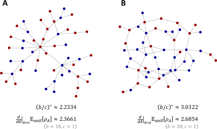
Figure 3: Two heterogeneous population structures of size $N=50$ evolving based on death-Birth updating. The population structure depicted in B is unequivocally better for the evolution of cooperation than that of A when $b=10$ and $c=1$ because selection results in a greater improvement to a rare cooperator’s fixation probability. This result holds despite the fact that the critical benefit-to-cost ratio of B is greater than it is for A, which means that the condition under which cooperators can thrive on B is stricter than that of A. It follows that a comparison between population structures based on which one is better for the evolution of cooperation cannot be made based on the critical ratios alone.

9 Discussion

In this study, we have analyzed the fixation probability of a mutant type under weak selection, for a broad class of evolutionary models and arbitrary initial conditions. The main result, Theorem 2, gives a first-order expansion of the fixation probability of $A$, $\rho_{A}\left(\bm{\xi}\right)$, in the selection intensity $\delta$, for any initial configuration, $\bm{\xi}$. This expansion has three main ingredients: (i) reproductive value, $\pi_{i}$, which quantifies the expected contribution of $i$ to future generations; (ii) neutral sojourn times, $\eta_{I}^{\bm{\xi}}$, which may be interpreted in terms of the mean number of steps in which all individuals in $I$ have type $A$ prior to absorption, given that the initial state of the population is $\bm{\xi}$; and (iii) Fourier coefficients, $c_{I}^{ij}$, of first-order effects of the probability that $i$ replaces $j$ in one update step.

It follows from Theorem 2 that the complexity of calculating this first-order expansion is $O\left(N^{3\left(D+1\right)}\right)$, where $D$ is the degree of the process. Actually, by the work of Le Gall (2012), this complexity is (in theory) $O\left(N^{2.373\left(D+1\right)}\right)$. This bound can be further improved in some cases by taking into account structural properties of the population, as we observed in the case of death-Birth updating on a regular graph. In any case, for fixed degree $D$, the system size exhibits polynomial growth in $N$, whereas the number of states in the evolutionary process grows exponentially in $N$.

The neutral sojourn times, $\eta_{I}^{\bm{\xi}}$ and variants thereof, play a central role in our method. Their interpretation is therefore a question of interest. From Eq. (36), we can see that $-\eta_{I}^{\bm{\xi}}=\left\langle\mathbf{x}_{I}-\widehat{x}\right\rangle_{\bm{\xi}}^{\circ}$ is a measure of the tendency for all individuals in $I$ have type $A$, under neutral drift from initial state $\bm{\xi}$. In the case of a uniform initial distribution $\mu_{A}$ (Example 1), $\eta_{I}^{\mu_{A}}$ is proportional to the expected time for the coalescent process $\mathcal{C}$ to reach a singleton set (coalesce) starting from set $I$.

The utility of our framework is illustrated by the application to evolutionary dynamics on graphs in Sections 7 and 8. In particular, Proposition 4 provides the weak-selection expansion of fixation probabilities for the donation game with arbitrary graph and initial configuration. This result unifies and generalizes the main results of Chen et al. (2016) (who considered only regular graphs) as well as Allen et al. (2017) (who considered only uniform initialization).

From these results, one can derive many of the well-known results on critical benefit-to-cost ratios for cooperation to be favored in social dilemmas (Ohtsuki et al., 2006; Taylor et al., 2007; Chen, 2013; Allen and Nowak, 2014; Fotouhi et al., 2018). Moreover, they provide more information than just when weak selection favors a particular trait; they also determine how much, based on the magnitude of $\frac{d}{d\delta}\Big{|}_{\delta=0}\rho_{A}$, which can lead to more nuanced comparisons of population structures based on their ability to promote a trait (Section 8.3). The magnitude of $\frac{d}{d\delta}\Big{|}_{\delta=0}\rho_{A}$ has been explored considerably less than its sign, and our results allow this question to be explored for quite a large class of evolutionary update rules, population structures, and initial configurations.

Our results on fixation probabilities apply to finite populations of a given size. It would be interesting to connect these results to the considerable body of theory for large populations (Kimura, 1962; Roze and Rousset, 2003; Traulsen et al., 2006; Cox and Durrett, 2016; Chen, 2018), by analyzing the large-population ($N\to\infty$) asymptotics of our results such as Eq. (34). However, a number of challenges arise. First, unless one places a bound on the degree of the process, the number of terms in first-order part of Eq. (34) grows exponentially with $N$. Second, since Eq. (34) is itself an expansion for weak selection ($\delta\ll 1$), one must consider the relationship between $N$ and $\delta$ as $N\to\infty$ and $\delta\to 0$. These two limits are known to be non-interchangeable, even in the relatively simple case of two-player games in a well-mixed population (Sample and Allen, 2017). However, neither of these challenges appears insurmountable, and addressing them is an important goal for future work.

References

- Adlam et al. (2015) B. Adlam, K. Chatterjee, and M. A. Nowak. Amplifiers of selection. Proceedings of the Royal Society A: Mathematical, Physical and Engineering Science, 471(2181):20150114, 2015. doi: 10.1098/rspa.2015.0114.
- Allen and McAvoy (2019) B. Allen and A. McAvoy. A mathematical formalism for natural selection with arbitrary spatial and genetic structure. Journal of Mathematical Biology, 78(4):1147–1210, 2019. doi: 10.1007/s00285-018-1305-z.
- Allen and Nowak (2014) B. Allen and M. A. Nowak. Games on graphs. EMS Surveys in Mathematical Sciences, 1(1):113–151, 2014. doi: 10.4171/emss/3.
- Allen and Tarnita (2014) B. Allen and C. E. Tarnita. Measures of success in a class of evolutionary models with fixed population size and structure. Journal of Mathematical Biology, 68(1-2):109–143, 2014. doi: 10.1007/s00285-012-0622-x.
- Allen et al. (2015) B. Allen, C. Sample, Y. Dementieva, R. C. Medeiros, C. Paoletti, and M. A. Nowak. The Molecular Clock of Neutral Evolution Can Be Accelerated or Slowed by Asymmetric Spatial Structure. PLOS Computational Biology, 11(2):e1004108, 2015. doi: 10.1371/journal.pcbi.1004108.
- Allen et al. (2017) B. Allen, G. Lippner, Y.-T. Chen, B. Fotouhi, N. Momeni, S.-T. Yau, and M. A. Nowak. Evolutionary dynamics on any population structure. Nature, 544(7649):227–230, 2017. doi: 10.1038/nature21723.
- Allen et al. (2019) B. Allen, G. Lippner, and M. A. Nowak. Evolutionary games on isothermal graphs. Nature Communications, 10(1):5107, 2019. doi: 10.1038/s41467-019-13006-7.
- Allen et al. (2020) B. Allen, C. Sample, R. Jencks, J. Withers, P. Steinhagen, L. Brizuela, J. Kolodny, D. Parke, G. Lippner, and Y. A. Dementieva. Transient amplifiers of selection and reducers of fixation for death-Birth updating on graphs. PLOS Computational Biology, 16(1):e1007529, 2020. doi: 10.1371/journal.pcbi.1007529.
- Antal et al. (2006) T. Antal, S. Redner, and V. Sood. Evolutionary Dynamics on Degree-Heterogeneous Graphs. Physical Review Letters, 96(18), 2006. doi: 10.1103/physrevlett.96.188104.
- Blume (1993) L. E. Blume. The Statistical Mechanics of Strategic Interaction. Games and Economic Behavior, 5(3):387–424, 1993. doi: 10.1006/game.1993.1023.
- Boros and Hammer (2002) E. Boros and P. L. Hammer. Pseudo-Boolean optimization. Discrete Applied Mathematics, 123(1-3):155–225, 2002. doi: 10.1016/s0166-218x(01)00341-9.
- Broom and Rychtář (2008) M. Broom and J. Rychtář. An analysis of the fixation probability of a mutant on special classes of non-directed graphs. Proceedings of the Royal Society A: Mathematical, Physical and Engineering Sciences, 464(2098):2609–2627, 2008. doi: 10.1098/rspa.2008.0058.
- Broom et al. (2011) M. Broom, J. Rychtář, and B. T. Stadler. Evolutionary Dynamics on Graphs - the Effect of Graph Structure and Initial Placement on Mutant Spread. Journal of Statistical Theory and Practice, 5(3):369–381, 2011. doi: 10.1080/15598608.2011.10412035.
- Chen (2013) Y.-T. Chen. Sharp benefit-to-cost rules for the evolution of cooperation on regular graphs. The Annals of Applied Probability, 23(2):637–664, 2013. doi: 10.1214/12-aap849.
- Chen (2018) Y.-T. Chen. Wright-fisher diffusions in stochastic spatial evolutionary games with death–birth updating. The Annals of Applied Probability, 28(6):3418–3490, 2018. doi: 10.1214/18-aap1390.
- Chen et al. (2016) Y.-T. Chen, A. McAvoy, and M. A. Nowak. Fixation Probabilities for Any Configuration of Two Strategies on Regular Graphs. Scientific Reports, 6(1), 2016. doi: 10.1038/srep39181.
- Cox (1989) J. T. Cox. Coalescing random walks and voter model consensus times on the torus in . Annals of Probability, 17(4):1333–1366, 1989. doi: 10.1214/aop/1176991158.
- Cox and Durrett (2016) J. T. Cox and R. Durrett. Evolutionary games on the torus with weak selection. Stochastic Processes and their Applications, 126(8):2388–2409, 2016. doi: 10.1016/j.spa.2016.02.004.
- Cuesta et al. (2017) F. A. Cuesta, P. G. Sequeiros, and Á. L. Rojo. Suppressors of selection. PLOS One, 12(7):e0180549, 2017. doi: 10.1371/journal.pone.0180549.
- Cuesta et al. (2018) F. A. Cuesta, P. G. Sequeiros, and Á. L. Rojo. Evolutionary regime transitions in structured populations. PLOS One, 13(11):e0200670, 2018. doi: 10.1371/journal.pone.0200670.
- Débarre et al. (2014) F. Débarre, C. Hauert, and M. Doebeli. Social evolution in structured populations. Nature Communications, 5, 2014. doi: 10.1038/ncomms4409.
- Der et al. (2011) R. Der, C. L. Epstein, and J. B. Plotkin. Generalized population models and the nature of genetic drift. Theoretical Population Biology, 80(2):80–99, 2011. doi: 10.1016/j.tpb.2011.06.004.
- Ewens (2004) W. J. Ewens. Mathematical Population Genetics. Springer New York, 2004. doi: 10.1007/978-0-387-21822-9.
- Fisher (1930) R. A. Fisher. The Genetical Theory of Natural Selection. Clarendon Press, 1930. doi: 10.5962/bhl.title.27468.
- Fotouhi et al. (2018) B. Fotouhi, N. Momeni, B. Allen, and M. A. Nowak. Conjoining uncooperative societies facilitates evolution of cooperation. Nature Human Behaviour, 2(7):492–499, 2018. doi: 10.1038/s41562-018-0368-6.
- Fudenberg and Imhof (2006) D. Fudenberg and L. A. Imhof. Imitation processes with small mutations. Journal of Economic Theory, 131(1):251–262, 2006. doi: 10.1016/j.jet.2005.04.006.
- Grabisch et al. (2000) M. Grabisch, J.-L. Marichal, and M. Roubens. Equivalent Representations of Set Functions. Mathematics of Operations Research, 25(2):157–178, 2000. doi: 10.1287/moor.25.2.157.12225.
- Haldane (1927) J. B. S. Haldane. A mathematical theory of natural and artificial selection, part V: Selection and mutation. In Mathematical Proceedings of the Cambridge Philosophical Society, volume 23, pages 838–844. Cambridge University Press, 1927. doi: 10.1017/S0305004100015644.
- Hammer and Rudeanu (1968) P. L. Hammer and S. Rudeanu. Boolean Methods in Operations Research and Related Areas. Springer Berlin Heidelberg, 1968. doi: 10.1007/978-3-642-85823-9.
- Hauert and Doebeli (2004) C. Hauert and M. Doebeli. Spatial structure often inhibits the evolution of cooperation in the snowdrift game. Nature, 428(6983):643–646, 2004. doi: 10.1038/nature02360.
- Hindersin and Traulsen (2014) L. Hindersin and A. Traulsen. Counterintuitive properties of the fixation time in network-structured populations. Journal of The Royal Society Interface, 11(99), 2014. doi: 10.1098/rsif.2014.0606.
- Hindersin and Traulsen (2015) L. Hindersin and A. Traulsen. Most Undirected Random Graphs Are Amplifiers of Selection for Birth-Death Dynamics, but Suppressors of Selection for Death-Birth Dynamics. PLOS Computational Biology, 11(11):e1004437, 2015. doi: 10.1371/journal.pcbi.1004437.
- Hindersin et al. (2016) L. Hindersin, M. Möller, A. Traulsen, and B. Bauer. Exact numerical calculation of fixation probability and time on graphs. Biosystems, 150:87–91, 2016. doi: 10.1016/j.biosystems.2016.08.010.
- Imhof and Nowak (2006) L. A. Imhof and M. A. Nowak. Evolutionary game dynamics in a Wright-Fisher process. Journal of Mathematical Biology, 52(5):667–681, 2006. doi: 10.1007/s00285-005-0369-8.
- Kaveh et al. (2015) K. Kaveh, N. L. Komarova, and M. Kohandel. The duality of spatial death-birth and birth-death processes and limitations of the isothermal theorem. Royal Society Open Science, 2(4):140465–140465, 2015. doi: 10.1098/rsos.140465.
- Kimura (1962) M. Kimura. On the Probability of Fixation of Mutant Genes in a Population. Genetics, 47(6):713–719, 1962.
- Kingman (1982) J. F. C. Kingman. The coalescent. Stochastic Processes and their Applications, 13(3):235–248, 1982. doi: 10.1016/0304-4149(82)90011-4.
- Le Gall (2012) F. Le Gall. Faster Algorithms for Rectangular Matrix Multiplication. In 2012 IEEE 53rd Annual Symposium on Foundations of Computer Science. IEEE, 2012. doi: 10.1109/focs.2012.80.
- Lessard and Ladret (2007) S. Lessard and V. Ladret. The probability of fixation of a single mutant in an exchangeable selection model. Journal of Mathematical Biology, 54(5):721–744, 2007. doi: 10.1007/s00285-007-0069-7.
- Lieberman et al. (2005) E. Lieberman, C. Hauert, and M. A. Nowak. Evolutionary dynamics on graphs. Nature, 433(7023):312–316, 2005. doi: 10.1038/nature03204.
- Liggett (1985) T. M. Liggett. Interacting Particle Systems. Springer New York, 1985. doi: 10.1007/978-1-4613-8542-4.
- Maciejewski (2014) W. Maciejewski. Reproductive value in graph-structured populations. Journal of Theoretical Biology, 340:285–293, 2014. doi: 10.1016/j.jtbi.2013.09.032.
- Maciejewski et al. (2014) W. Maciejewski, F. Fu, and C. Hauert. Evolutionary game dynamics in populations with heterogenous structures. PLoS Computational Biology, 10(4):e1003567, 2014. doi: 10.1371/journal.pcbi.1003567.
- McAvoy and Hauert (2016) A. McAvoy and C. Hauert. Structure coefficients and strategy selection in multiplayer games. Journal of Mathematical Biology, 72(1):203–238, 2016. doi: 10.1007/s00285-015-0882-3.
- McAvoy et al. (2020) A. McAvoy, B. Allen, and M. A. Nowak. Social goods dilemmas in heterogeneous societies. Nature Human Behaviour, 4(8):819–831, 2020. doi: 10.1038/s41562-020-0881-2.
- McCandlish et al. (2015) D. M. McCandlish, C. L. Epstein, and J. B. Plotkin. Formal properties of the probability of fixation: Identities, inequalities and approximations. Theoretical Population Biology, 99:98–113, 2015. doi: 10.1016/j.tpb.2014.11.004.
- Möller et al. (2019) M. Möller, L. Hindersin, and A. Traulsen. Exploring and mapping the universe of evolutionary graphs identifies structural properties affecting fixation probability and time. Communications Biology, 2(1):137, 2019. doi: 10.1038/s42003-019-0374-x.
- Monk et al. (2014) T. Monk, P. Green, and M. Paulin. Martingales and fixation probabilities of evolutionary graphs. Proceedings of the Royal Society A: Mathematical, Physical and Engineering Sciences, 470(2165):20130730–20130730, 2014. doi: 10.1098/rspa.2013.0730.
- Moran (1958) P. A. P. Moran. Random processes in genetics. Mathematical Proceedings of the Cambridge Philosophical Society, 54(01):60, 1958. doi: 10.1017/s0305004100033193.
- Nathanson et al. (2009) C. G. Nathanson, C. E. Tarnita, and M. A. Nowak. Calculating Evolutionary Dynamics in Structured Populations. PLoS Computational Biology, 5(12):e1000615, 2009. doi: 10.1371/journal.pcbi.1000615.
- Nowak and May (1992) M. A. Nowak and R. M. May. Evolutionary games and spatial chaos. Nature, 359(6398):826–829, 1992. doi: 10.1038/359826a0.
- Nowak et al. (2004) M. A. Nowak, A. Sasaki, C. Taylor, and D. Fudenberg. Emergence of cooperation and evolutionary stability in finite populations. Nature, 428(6983):646–650, 2004. doi: 10.1038/nature02414.
- Nowak et al. (2009) M. A. Nowak, C. E. Tarnita, and T. Antal. Evolutionary dynamics in structured populations. Philosophical Transactions of the Royal Society B: Biological Sciences, 365(1537):19–30, 2009. doi: 10.1098/rstb.2009.0215.
- Ohtsuki (2014) H. Ohtsuki. Evolutionary dynamics of -player games played by relatives. Philosophical Transactions of the Royal Society B: Biological Sciences, 369(1642):20130359–20130359, 2014. doi: 10.1098/rstb.2013.0359.
- Ohtsuki et al. (2006) H. Ohtsuki, C. Hauert, E. Lieberman, and M. A. Nowak. A simple rule for the evolution of cooperation on graphs and social networks. Nature, 441(7092):502–505, 2006. doi: 10.1038/nature04605.
- Patwa and Wahl (2008) Z. Patwa and L. M. Wahl. The fixation probability of beneficial mutations. Journal of The Royal Society Interface, 5(28):1279–1289, 2008. doi: 10.1098/rsif.2008.0248.
- Pavlogiannis et al. (2018) A. Pavlogiannis, J. Tkadlec, K. Chatterjee, and M. A. Nowak. Construction of arbitrarily strong amplifiers of natural selection using evolutionary graph theory. Communications Biology, 1(1), 2018. doi: 10.1038/s42003-018-0078-7.
- Peña et al. (2016) J. Peña, B. Wu, and A. Traulsen. Ordering structured populations in multiplayer cooperation games. Journal of The Royal Society Interface, 13(114):20150881, 2016. doi: 10.1098/rsif.2015.0881.
- Rousset (2003) F. Rousset. A Minimal Derivation of Convergence Stability Measures. Journal of Theoretical Biology, 221(4):665–668, 2003. doi: 10.1006/jtbi.2003.3210.
- Roze and Rousset (2003) D. Roze and F. Rousset. Selection and drift in subdivided populations: a straightforward method for deriving diffusion approximations and applications involving dominance, selfing and local extinctions. Genetics, 165(4):2153–2166, 2003.
- Sample and Allen (2017) C. Sample and B. Allen. The limits of weak selection and large population size in evolutionary game theory. Journal of Mathematical Biology, 75(5):1285–1317, 2017. doi: 10.1007/s00285-017-1119-4.
- Santos and Pacheco (2005) F. C. Santos and J. M. Pacheco. Scale-free networks provide a unifying framework for the emergence of cooperation. Physical Review Letters, 95(9):098104, 2005. doi: 10.1103/physrevlett.95.098104.
- Santos et al. (2008) F. C. Santos, M. D. Santos, and J. M. Pacheco. Social diversity promotes the emergence of cooperation in public goods games. Nature, 454(7201):213–216, 2008. doi: 10.1038/nature06940.
- Sigmund (2010) K. Sigmund. The calculus of selfishness. Princeton University Press, 2010. doi: 10.1515/9781400832255.
- Szabó and Fáth (2007) G. Szabó and G. Fáth. Evolutionary games on graphs. Physics Reports, 446(4-6):97–216, 2007. doi: 10.1016/j.physrep.2007.04.004.
- Tarnita and Taylor (2014) C. E. Tarnita and P. D. Taylor. Measures of Relative Fitness of Social Behaviors in Finite Structured Population Models. The American Naturalist, 184(4):477–488, 2014. doi: 10.1086/677924.
- Tarnita et al. (2009) C. E. Tarnita, H. Ohtsuki, T. Antal, F. Fu, and M. A. Nowak. Strategy selection in structured populations. Journal of Theoretical Biology, 259(3):570–581, 2009. doi: 10.1016/j.jtbi.2009.03.035.
- Taylor et al. (2004) C. Taylor, D. Fudenberg, A. Sasaki, and M. A. Nowak. Evolutionary game dynamics in finite populations. Bulletin of Mathematical Biology, 66(6):1621–1644, 2004. doi: 10.1016/j.bulm.2004.03.004.
- Taylor (1990) P. D. Taylor. Allele-Frequency Change in a Class-Structured Population. The American Naturalist, 135(1):95–106, 1990. doi: 10.1086/285034.
- Taylor et al. (2007) P. D. Taylor, T. Day, and G. Wild. Evolution of cooperation in a finite homogeneous graph. Nature, 447(7143):469–472, 2007. doi: 10.1038/nature05784.
- Tkadlec et al. (2019) J. Tkadlec, A. Pavlogiannis, K. Chatterjee, and M. A. Nowak. Population structure determines the tradeoff between fixation probability and fixation time. Communications Biology, 2, 2019. doi: 10.1038/s42003-019-0373-y.
- Tkadlec et al. (2020) J. Tkadlec, A. Pavlogiannis, K. Chatterjee, and M. A. Nowak. Limits on amplifiers of natural selection under death-birth updating. PLOS Computational Biology, 16(1):e1007494, 2020. doi: 10.1371/journal.pcbi.1007494.
- Traulsen and Hauert (2010) A. Traulsen and C. Hauert. Stochastic Evolutionary Game Dynamics. In Reviews of Nonlinear Dynamics and Complexity, pages 25–61. Wiley-Blackwell, 2010. doi: 10.1002/9783527628001.ch2.
- Traulsen et al. (2006) A. Traulsen, J. M. Pacheco, and L. A. Imhof. Stochasticity and evolutionary stability. Physical Review E, 74(2):021905, 2006. doi: 10.1103/physreve.74.021905.
- Van Cleve (2015) J. Van Cleve. Social evolution and genetic interactions in the short and long term. Theoretical Population Biology, 103:2–26, 2015. doi: 10.1016/j.tpb.2015.05.002.
- Voorhees (2013) B. Voorhees. Birth-death fixation probabilities for structured populations. Proceedings of the Royal Society A: Mathematical, Physical and Engineering Sciences, 469(2153):20120248, 2013. doi: 10.1098/rspa.2012.0248.
- Wakeley (2016) J. Wakeley. Coalescent Theory: An Introduction. Macmillan Learning, 2016.
- Wright (1931) S. Wright. Evolution in Mendelian populations. Genetics, 16:97–159, 1931.