Development and testing of an unstructured mesh method for whole plasma gyrokinetic simulations in realistic tokamak geometry
Abstract
In this work, we have formulated and implemented a mixed unstructured mesh-based finite element (FE)–Fourier decomposition scheme for gyrokinetic simulations in realistic tokamak geometry. An efficient particle positioning (particle-triangle mapping) scheme for the charge deposition and field scattering using an intermediate grid as the search index for triangles has been implemented and a significant speed-up by a factor of is observed as compared with the brute force scheme for a medium-size simulation. The TRIMEG (TRIangular MEsh based Gyrokinetic) code has been developed. As an application, the ion temperature gradient (ITG) mode is simulated using the simplified gyrokinetic Vlasov-Poisson model. Our simulation and that using the ORB5 code for the DIII-D Cyclone case show reasonable agreement. As an additional application, ITG simulations using an ASDEX Upgrade equilibrium have been performed with density and temperature gradient profiles similar to the Cyclone case. Capabilities of the TRIMEG code for simulations with realistic experimental equilibria in the plasma core and in the whole plasma volume with open field lines are demonstrated.
I Introduction
Gyrokinetic simulations play an important role in predicting the transport level due to neoclassical physics or turbulence lee1983gyrokinetic ; lin1995gyrokinetic ; lin1998turbulent ; wang2015distinct ; ku2009full ; jenko2000electron ; dorland2000electron . One of the leading methods is the particle-in-cell (PIC) method. Numerous PIC codes, such as GTC lin1995gyrokinetic , GEM parker2000electromagnetic , ORB5 jolliet2007global , have been developed for simulations in the core of the tokamak plasmas. Edge plasma simulations have attracted significant attention in recent years due to their connection to, e.g., the high confinement regime of tokamak plasmas; the prediction of the divertor heat-flux width of ITER chang2017gyrokinetic ; edge localized mode (ELM) control huysmans2007mhd . In order to simulate the edge physics, besides comprehensive physics models qin2006general ; scott2006edge , numerical schemes such as finite element methods for unstructured meshes in XGC ku2009full ; ferraro2010ideal , GTS wang2015distinct and GTC/GTC-X nishimura2006finite ; bao2019global and multiple patches of structured meshes in JOREK huysmans2007mhd have been developed in order to treat the open field line (OFL) region. While whole plasma simulations for neoclassical transport, ELMs and micro-turbulence have been reported and various numerical schemes have been developed for treating the OFL geometry ku2009full ; chang2017gyrokinetic ; huysmans2007mhd ; nishimura2006finite ; de2019kinetic ; vugt2019kinetic , there is still space to understand the features of different schemes, such as the particle-in-Fourier method (cf. [19; 20] and references therein), and thus to optimize the efficiency and the fidelity of the whole volume simulation.
In this work, we developed the mixed unstructured mesh based finite element–Fourier decomposition scheme, i.e., the mixed particle-in-cell-particle-in-Fourier (PIC-PIF) scheme, for gyrokinetic simulations in general tokamak geometry, including the OFL region. In addition, an efficient particle positioning scheme for the charge deposition and the field gathering using an intermediate grid as the search index for triangles has been implemented. This work is organized as follows. In Section II, the physics model and numerical schemes are given. In Section III, we perform convergence/scaling studies and simulations of ion temperature gradient (ITG) modes using (I) the concentric circular magnetic geometry and the DIII-D cyclone parameters and (II) the AUG realistic magnetic equilibrium and analytical density and temperature profiles. In IV, conclusions and an outlook are given.
II Physics model and numerical methods
In the following, we will define the normalization in Section II.1. In Sections II.2–II.4, we will describe the three basic classes in the code, namely, the equilibrium, particle and field classes. We then describe the numerical methods in Section II.5. While the equations of motion for the guiding center, the weight equation, and the gyrokinetic Poisson equation (in the long wavelength limit) in this work are the same as or are the simplified version of other codes such as ORB5 jolliet2009gyrokinetic ; lanti2019orb5arxiv , the mixed unstructured mesh-based finite element-Fourier decomposition scheme makes our work different from ORB5. In ORB5, the OFL region is not included in either the particle pusher or the field solver. The mixed approach in this work thus also serves as a potential candidate for the extension of the present codes such as ORB5 towards whole plasma volume simulations. The details related to the finite element and unstructured meshes are described in another work for circular tokamak geometry lu2019mixed and will be omitted in this work.
II.1 Normalization
Normalization units are defined and physics quantities are normalized to the normalization units. The length unit is . The velocity unit is , where , is the reference temperature, is the the mass of hydrogen, the subscripts ‘’ and ‘’ indicate “normalization” and “hydrogen” respectively. For each particle species s, is used as the velocity unit for the particle initialization according to a Maxwellian distribution function while unit conversion to the normalization unit is performed in the equations of motion for the guiding center and the field equation. The time unit is . The magnetic field unit is .
II.2 The coordinates and the equilibrium
In the right-handed coordinates and , where is the poloidal flux function, using the EFIT convention, the magnetic field is represented as
| (1) |
where is the poloidal current function. In the coordinates, the safety factor is defined as , where . The equilibrium variables are constructed using B-splines in the plane of the coordinates. Equilibrium variables such as , , and their derivatives in and directions can be obtained using the B-spline subroutines.
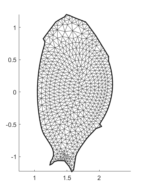
The hybrid coordinates and are used. On the one hand, the user specified computation grids are aligned along the magnetic flux surface using the coordinate, or, if the OFL region is included, along the plasma boundary; the refinement grids are generated when the Delaunay refinement algorithm is called for the generation of the unstructured meshes shewchuk2002delaunay . The refinement grids using the Delaunay algorithm are not necessarily along the magnetic flux surface but it is a widely used technique for the improvement of the mesh quality. Two cases of the grids and the unstructured meshes for the simulations in Section III are shown in Fig. 1. More details about the finite element for the unstructured meshes are in another work lu2019mixed . On the other hand, in order to treat the open field line geometry, the equations for the field and particles are solved in coordinates. In coordinates, the equilibrium magnetic field is expressed as
| (2) |
TRIMEG relies on the B-Spline subroutines for the interpolation of and accurately and keeps the error in at a low level. For simulations in this manuscript, we use as the grid numbers in R and Z directions for the equilibrium construction. In the relevant simulation domain, the error in is well below with the upper limit of . The parallel derivative is
| (3) |
where is the perturbed electrostatic scalar potential, , and .
The field-aligned coordinates are constructed as another option for the calculation of the parallel derivatives in addition to Eq. 3. Along the magnetic field line , the auxiliary Clebsch coordinates are determined by
| (4) | |||||
| (5) | |||||
| (6) |
where labels a magnetic field line and can be taken as at for convenience and is the coordinate along . The parallel derivative using these Clebsch coordinates is
| (7) |
For parallel derivatives of high (toroidal mode number) field-aligned modes, Eq. 7 can provide high accuracy compared with Eq. 3.
Since or coordinates are used for solving all equations in the code except when the grids are initialized according to , and the safety factor defined in does not appear explicitly but , and are used directly in our equations, the singularity of the at the X point does not appear in any equation solved in TRIMEG. The auxiliary coordinates maintain the high accuracy of the parallel derivative calculation for high field-aligned modes and are similar to the flux-coordinate independent approach hariri2013flux ; stegmeir2016field . Discussions related to the flux coordinates and singularity of the safety factor at the X point can be found in [27] and references therein.
II.3 Particles
II.3.1 Equations of motion
In this work, we focus on electrostatic simulations. In order to describe the particle guiding center motion, we follow the canonical Hamiltonian equations white1990canonical . Using as the guiding center coordinates, the equations of motion are as follows,
| (8) | |||||
| (9) |
where , , is the charge number, is the Hamiltonian, and . The equations of motion above are equivalent to those adopted in XGC ku2009full ,
| (10) | |||||
| (11) |
where is related to the higher order corrections.
The variables can be written as
| (12) | |||||
| (13) |
where the subscripts and indicate the motion of the guiding center in equilibrium and that due to the electrostatic field. In coordinates, the contravariant components of the velocity are calculated for different terms.
-
1.
Magnetic drift
(14) (15) (16) The dominant terms of the equations of motion are obtained by omitting the terms of the order of and of , where , . In coordinates, the dominant terms in the equations of motion are
which, noticing that , where is the unit vector in the toroidal direction, and , can be further reduced to,
(17) -
2.
drift . Generally, drift is contributed from the equilibrium scalar potential and the perturbed scalar potential , i.e., . In this work, we only consider the latter one, i.e.,
(18) (19) (20) where indicates a gyro average. In TRIMEG, the four point gyro average scheme is adopted. For the calculation of , where indicates or its derivative in or direction, and are calculated and the average value is obtained. The dominant term is
(21) where and are the unit vectors in the and directions.
-
3.
Parallel acceleration
(22) The dominant term is
(23)
The simplification of other terms such as and is trivial and is omitted.
II.3.2 Weight equation
The gyrokinetic Vlasov equation for the evolution of the perturbed distribution function is
| (24) |
where
The weight of the markers is defined to represent the perturbed distribution function,
| (25) | |||||
where and are the total numbers of the physical particles and numerical markers respectively and the subscript is the marker index. Defining as the phase space volume occupied by the marker , Eq. 25 yields
| (26) |
and Eq. 24 gives
| (27) |
The above definition is the same as that in ORB5 jolliet2007global ; lanti2019orb5arxiv . However, in this work, for the sake of simplicity, we load the markers with the distribution function the same as that of the physical particles, i.e.,
| (28) |
then
| (29) |
where is the gyro angle. Equations 27, 28 and 29 yield
| (30) |
The perturbed density in a small volume is calculated from the marker weight in
| (31) |
where is the volume averaged density. For unstructured meshes, the volume is centered around a vertex and is calculated using , where is a triangular prism which extends along the direction. Using the particle-in-Fourier method in the toroidal direction, we have for each toroidal mode number ,
| (32) |
where is the projection of in the plane.
II.4 Field equation
The gyrokinetic Poisson equation with the long wavelength approximation is adopted in this work, i.e.,
| (33) |
Generally, the electron response is dominated by the adiabatic response. Thus, the electron response can be decomposed into the adiabatic and non adiabatic (NA) parts, i.e.,
| (34) |
where is the non-zonal component, i.e., , is the poloidal harmonic with , where is the poloidal mode number. Notice that the Fourier decomposition is used in the direction but the finite element method is used in the plane.
For , with the subscript omitted,
| (35) |
For ,
| (36) |
In this work, we focus on the modes while the studies involving components such as the geodesic acoustic mode will be reported in another separate work lu2019mixed .
II.5 Numerical methods
II.5.1 General description
This gyrokinetic Poisson-Vlasov system is implemented in Fortran. The field equation is solved using the finite element method for unstructured meshes. The sparse matrix corresponding to the gyrokinetic Poisson equation is solved using PETSc (Portable, Extensible Toolkit for Scientific Computation) balay2019petsc . The Runge-Kutta fourth order integrator is implemented for particles and coupled to the field solver. The Runge–Kutta fourth-order method is given by the following steps,
where , , is the time interval and is solved from Eq. 33 with obtained using for .
II.5.2 Particle positioning (deposition/gathering) scheme
When calculating the toroidal component of the charge density perturbation in Eq. 32 using marker weights in the so-called “charge deposition” stage, or when interpolating the field value at the particle position using the grid field value during the “field gathering” stage, the marker-triangle mapping, i.e., the particle positioning, needs to be treated. For the brute force particle position scheme, each triangle is checked for each marker whether the triangle contains the marker, which leads to a scale computational cost, where and are the marker and triangle numbers respectively. In this work, rectangular grids (“boxes”) are constructed in space and the box-triangle index is built when there is overlap between a box and a triangle . The mapping , is stored in the dynamically growing arrays for each box . For a given marker , the box which contains Marker is first found, i.e., the mapping is identified. Then using the box-triangle mapping , the corresponding triangle is identified. The computational cost is for markers, where is a constant number.
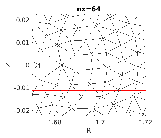
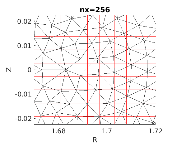
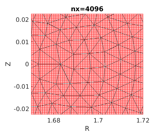
The intermediate boxes are generated in the simulation domain with given and , where and are the rectangular grid numbers in and directions respectively. One limit is , where is the radial grid number of the unstructured meshes. For (the box number is one), the positioning scheme is identical to the brute force scheme. The other limit is , for which the box size is much smaller than the triangle size. A typical case between these two limit cases is that with . These three cases are shown in Fig. 2. The computational speed-up versus the box size or will be studied in Sec. III.
III Numerical results
III.1 Parameters and simplifications for the simulation
In this section, two experimental cases are discussed. For numerical studies and benchmarks in Sections III.2 and III.3, the DIII-D Cyclone case is adopted, for which the parameters are the same as those in the benchmark work gorler2016intercode . The geometry with concentric circular magnetic flux surfaces is assumed. The nominal safety factor profile isgorler2016intercode
| (37) |
where . In Sections III.2 and III.3, an ad hoc equilibrium model is adopted. By assuming the following form of the safety factor profile,
| (38) |
where , the poloidal flux function can be obtained analytically bottino2007nonlinear ; lu2019mixed . The values of and the magnetic shear are matched to Eq. 37 at , i.e., , , where and are calculated at using Eq. 37. The temperature and density profiles indicated by and the corresponding normalized logarithmic gradients indicated by are given by
| (39) | |||||
| (40) |
where the subscript ‘c’ denotes the center of the gradient and the values of , etc are in Table 1.
For the studies using the realistic geometry in Section III.4, the ASDEX Upgrade (AUG) case with shot number 34924 at 3.600s is chosen. This is a typical discharge for the study of energetic particle and turbulence physics lauber2018strongly . In the simulation, we use the experimental equilibrium but use the analytical density and temperature profiles in Eq. 40, with the radial coordinate replaced with , where and are the poloidal magnetic flux function at the magnetic axis and at the last closed surface respectively. The purpose of this study is to test the capability of treating the realistic geometry with minimum technical complexity. The fully self consistent treatment of the density/temperature profile and the equilibrium will be addressed in another work.
Since our purpose is to study the mixed PIC-PIF scheme and the particle search scheme in this work and address the basic ITG mode problem in the whole plasma geometry with minimum complexity, we have made the following simplifications.
- 1.
-
2.
The equilibrium variation of , and in the gyrokinetic Poisson equation, Eq. 33, is ignored.
-
3.
The ITG instability drive in Eq. 40 for the weight equation is kept but the equilibrium variation in , and is omitted.
-
4.
A single toroidal harmonic is simulated without the nonlinear terms, even though the dominant nonlinear term for the ITG saturation is implemented in TRIMEG.
-
5.
The Dirichlet boundary condition is adopted for the gyrokinetic Poisson equation with at the boundary. The “absorbing boundary condition” for markers are adopted, i.e., the markers hitting the boundary are removed from the system.
-
6.
Adiabatic electron approximation is adopted, i.e., in Eq. 34.
-
7.
As the initial condition, markers with Maxwellian distribution are loaded in the simulation domain. Markers hitting the wall are removed (absorbing boundary condition). Since in this work, we only performed linear simulations, the marker distribution does not change after all absorbed markers are removed.
This simplified model can be replaced with a more comprehensive one by either future development of the TRIMEG code, or by implementing the finite element solver for unstructured meshes and the PIC-PIF scheme in other codes such as ORB5 and GTC.
| 0.5 | 0.36 | 180 | 1 | 1 | 6.69 | 2.23 | 0.3 |
III.2 Convergence and scaling studies
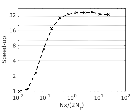
The effects of the rectangular box size on the computational cost in the particle positioning scheme are studied using a medium size case whose radial grid number is and the total marker number is 25.6 million. The brute force scheme () serves as the baseline and the speed-up for other values of is shown in Fig. 3. There is an optimal value of the box size with respect to the triangle size in the range of . The speed-up for are ; larger than those for other values of . For , each box contains a large number of triangles, as shown in Fig. 2 (left) and identifying the particle-triangle mapping consumes a significant amount of computing time. For , the particle positioning in the charge deposition and field gathering can cost of the total computing time. As increases and becomes larger than 1, the particle positioning consumption is reduced and the cost of the charge deposition and the field gathering is comparable to the particle pusher. For , the memory cost for storing the box-triangle mapping increases but without significant CPU cost, and thus only slows down the simulation slightly. Even as changes from 1024 to 8192, the speed-up decreases from 36.3 to 32.7, by only around .
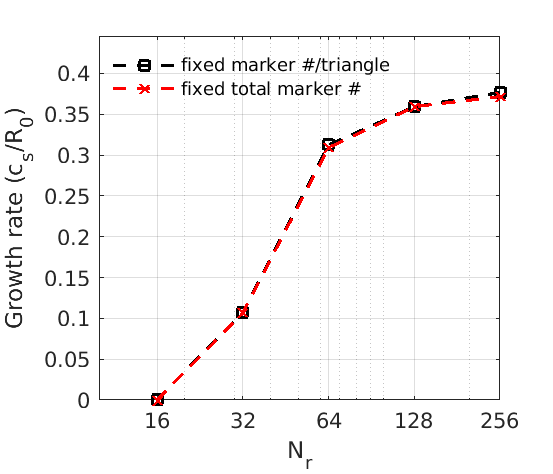
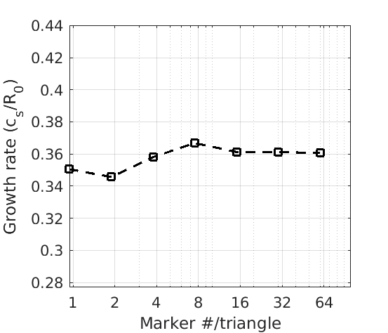
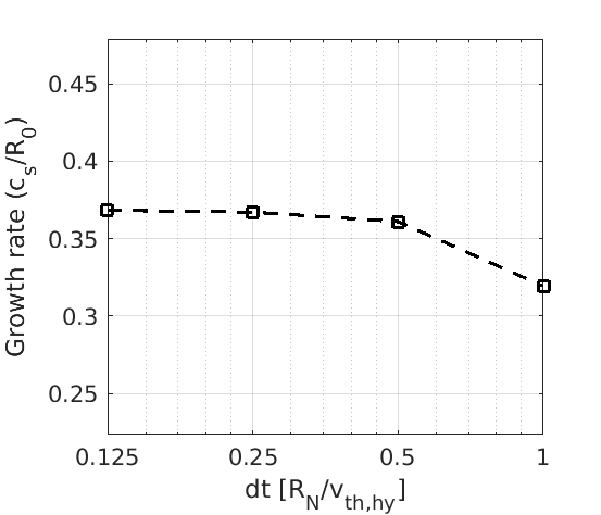
The convergence of the simulation results in terms of growth rate with respect to the radial grid number, the marker number per triangle and the time step size is studied. The convergence with respect to , marker number and time step size is shown in Fig. 4. For this mode, as shown in the left frame, from , the simulation starts to converge. The corresponding poloidal grid number per wave length . Note that the poloidal grid spacing is set to be close to the radial grid spacing. For the linear studies in this work, the mode structure is elongated along the radial direction and the minimum value of is determined by the grid number per wave length in poloidal direction, i.e., . In the middle frame, the results start to converge when the marker number per triangle . In the right frame, the simulation starts to converge for and becomes numerically unstable for .
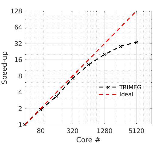
The parallel performance is tested for evaluating the scaling properties. The speed-up for the simulation with million markers with different numbers of cores is analyzed and shown in Fig. 5. Its comparison with the ideal scaling shows the good strong scaling for small to moderate core numbers (core number ). For even larger core numbers, the consumption of the field solver parallel communication can increase since the field solver is distributed over all cores. As a result, the deviation of the speed-up curve away from the ideal scaling becomes significant as the core number is larger than 1280.
III.3 ITG simulation using Cyclone parameters
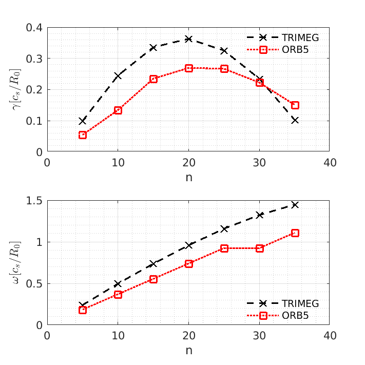
Following the convergence and scaling studies in Section III.2, ITG mode simulations using the Cyclone case parameters are performed. The growth rate and the frequency are shown in Fig. 6 and are compared with the ORB5 results noticing , where is the major radius. The agreement between the TRIMEG results and the ORB5 results is reasonable, noting the simplifications in TRIMEG as discussed in Sec. III.1. Nevertheless, considering the spatial scale separation between the equilibrium profile variation spatial scale , the mode structure radial envelope width and the single poloidal harmonic width , i.e., lu2012theoretical , the simulation from TRIMEG already captures the leading order solution. More comprehensive physics models will be implemented in the future.
III.4 ITG simulation using AUG equilibrium in the core plasma and in the whole plasma geometry
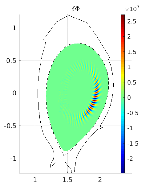
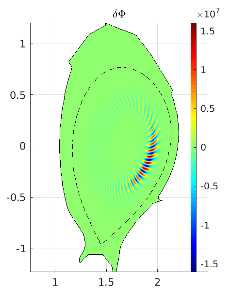
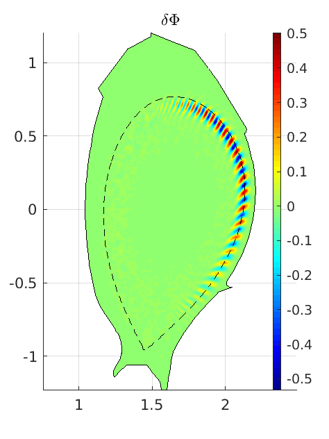
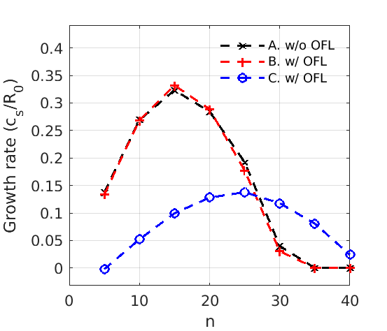
In this section, we perform simulations of ITG modes using the AUG equilibrium described in Section III.1. The main purpose is to demonstrate the capability of treating the realistic magnetic equilibrium from an experiment using TRIMEG. Three cases are defined in Table 2. The simulations without and with the open field line region are performed and compared as shown in Fig. 7 and Fig. 8. For Cases (A) and (B), the open field line plays a weak role on the core ITG mode due to the narrow envelope of the radial mode structure. As a result, the 2D mode structures and the growth rate are almost identical between these two cases. For Case C, the local variables at such as , , and the minor radius that determine the mode growth rate are different from (A) and (B). As a result, the growth rate curve is shifted due to the change in the finite Larmor radius / finite orbit width effects () and other effects. While the convergence of the simulation for the whole plasma volume is achieved, a benchmark with other codes with the treatment of the whole plasma geometry will be studied in the future. Missing physics in the TRIMEG code includes, but is not limited to, the fully nonlinear collision operator hager2016fully ; a more realistic boundary condition such as a sheath boundary condition cohen2004sheath ; boesl2019gyrokinetic ; the radial electric field consistent with neoclassical physics; and zonal flow physics. In addition, more comprehensive gyrokinetic/gyrofluid models for the edge also need to be considered scott2006edge ; qin2006general .
| Case | OFL | ||
|---|---|---|---|
| A | w/o | 0.5 | 0.3 |
| B | w/ | 0.5 | 0.3 |
| C | w/ | 1.0 | 0.1 |
IV Conclusion
In this work, the TRIMEG code has been developed based on the mixed unstructured mesh based FEM-Fourier decomposition scheme and the intermediate grid for the particle position. The parallel scalability of charge deposition and field gathering has been achieved and strong scaling up to moderate core numbers has been demonstrated. The benchmark with ORB5 using the DIII-D Cyclone test case shows reasonable agreement in terms of growth rate and frequency. The capability of treating the whole plasma volume is demonstrated by using an AUG magnetic equilibrium with an X-point and analytical density and temperature profiles. Futher development of the TRIMEG code for specific physics studies such as the mode structure symmetry breaking lu2017symmetry ; lu2018mode ; lu2018kinetic ; lu2019theoretical and for more comprehensive simulations including the wave-particle and wave-wave nonlinearities and multiple species will be explored in the future.
Acknowledgments
Simulations were performed on MPCDF computing systems. Suggestions from ORB5, EUTERPE, HMGC, GTC and GTS groups, discussion with B.D. Scott, D. Coster, A. Bierwage and support by National Natural Science Foundation of China under Grant No. 11605186 are appreciated by ZL. ZL thanks X. Wang for naming the code TRIMEG. Support by the ENR projects “NAT” and “MET” is acknowledged. This work has been carried out within the framework of the EUROfusion Consortium and has received funding from the Euratom research and training programme 2014-2018 and 2019-2020 under grant agreement No 633053. The views and opinions expressed herein do not necessarily reflect those of the European Commission.

References
- (1) WW Lee. Phys. Fluids, 26(2):556, 1983.
- (2) Z Lin, WM Tang, and WW Lee. Phys. Plasmas, 2(8):2975, 1995.
- (3) Z Lin, TS Hahm, WW Lee, WM Tang, and RB White. Science, 281(5384):1835, 1998.
- (4) WX Wang, S Ethier, Y Ren, S Kaye, J Chen, E Startsev, and Z Lu. Nucl. Fusion, 55(12):122001, 2015.
- (5) S Ku, CS Chang, and PH Diamond. Nucl. Fusion, 49(11):115021, 2009.
- (6) F Jenko, W Dorland, M Kotschenreuther, and BN Rogers. Phys. Plasmas, 7(5):1904, 2000.
- (7) W Dorland, F Jenko, Mike Kotschenreuther, and BN Rogers. Electron temperature gradient turbulence. Phys. Rev. Lett., 85(26):5579, 2000.
- (8) SE Parker, Y Chen, and CC Kim. Comput. Phys. Commun., 127(1):59–70, 2000.
- (9) S Jolliet, A Bottino, P Angelino, R Hatzky, TM Tran, BF Mcmillan, O Sauter, K Appert, Y Idomura, and L Villard. Comput. Phys. Commun., 177(5):409, 2007.
- (10) CS Chang, S Ku, A Loarte, V Parail, F Koechl, M Romanelli, R Maingi, JW Ahn, T Gray, J Hughes, et al. Nucl. Fusion, 57(11):116023, 2017.
- (11) GTA Huysmans and O Czarny. Nucl. Fusion, 47(7):659, 2007.
- (12) H Qin, RH Cohen, WM Nevins, and XQ Xu. Contrib. Plasma Phys., 46(7):477, 2006.
- (13) BD Scott. Contrib. Plasma Phys., 46(7):714, 2006.
- (14) NM Ferraro, SC Jardin, and PB Snyder. Phys. Plasmas, 17(10):102508, 2010.
- (15) Y Nishimura, Z Lin, JLV Lewandowski, and S Ethier. J. Comput. Phys., 214(2):657, 2006.
- (16) J Bao, CK Lau, Z Lin, HY Wang, DP Fulton, S Dettrick, and T Tajima. Phys. Plasmas, 26(4):042506, 2019.
- (17) S De, T Singh, A Kuley, J Bao, Z Lin, GY Sun, S Sharma, and A Sen. Phys. Plasmas, 26(8):082507, 2019.
- (18) D. C. van Vugt, G. T. A. Huijsmans, M. Hoelzl, and A. Loarte. Phys. Plasmas, 26(4):042508, 2019.
- (19) J Ameres. Stochastic and Spectral Particle Methods for Plasma Physics. PhD thesis, Technische Universität München, 2018.
- (20) N Ohana, A Jocksch, E Lanti, AL Scheinberg, S Brunner, C Gheller, and L Villard. In 17th European Fusion Theory Conference, 2017.
- (21) S Jolliet. Gyrokinetic particle-in-cell global simulations of ion-temperature-gradient and collisionless-trapped-electron-mode turbulence in tokamaks. EPFL thesis, 2009.
- (22) E Lanti, N Ohana, N Tronko, T Hayward-Schneider, A Bottino, BF McMillan, A Mishchenko, A Scheinberg, A Biancalani, P Angelino, et al. arXiv preprint arXiv:1905.01906, 2019.
- (23) ZX Lu, Ph Lauber, X Wang, A Bottino, A Mishchenko, and J Chen. The mixed unstructured fem-fourier decomposition scheme as a fast linear solver for studies of tokamak plasma waves and instabilities. to be submitted, 2019.
- (24) JR Shewchuk. Computational geometry, 22(1):21, 2002.
- (25) F Hariri and M Ottaviani. Comput. Phys. Commun., 184(11):2419–2429, 2013.
- (26) A. Stegmeir, D. Coster, O. Maj, K. Hallatschek, and K. Lackner. The field line map approach for simulations of magnetically confined plasmas. Comput. Phys. Commun., 198:139, 2016.
- (27) ZX Lu, F Zonca, and A Cardinali. Phys. Plasmas, 19(4):042104, 2012.
- (28) RB White. Phys. Fluids B, 2(4):845, 1990.
- (29) S Balay, S Abhyankar, M Adams, J Brown, P Brune, K Buschelman, L Dalcin, A Dener, V Eijkhout, W Gropp, et al. Petsc users manual. 2019.
- (30) T Görler, N Tronko, WA Hornsby, A Bottino, R Kleiber, C Norscini, V Grandgirard, F Jenko, and E Sonnendrücker. Phys. Plasmas, 23(7):072503, 2016.
- (31) A Bottino, AG Peeters, R Hatzky, S Jolliet, BF McMillan, TM Tran, and L Villard. Phys. Plasmas, 14(1):010701, 2007.
- (32) P Lauber, B Geiger, G Papp, GI Pokol, A Biancalani, X Wang, Z Lu, P Pölöskei, A Bottino, F Palermo, et al. Strongly non-linear energetic particle dynamics in ASDEX Upgrade scenarios with core impurity accumulation. In 27th IAEA Fusion Energy Conference (FEC 2018), 2018.
- (33) R Hager, ES Yoon, S Ku, EF D’Azevedo, PH Worley, and CS Chang. J. Comput. Phys., 315:644, 2016.
- (34) RH Cohen and DD Ryutov. Contrib. Plasma Phys., 44(1):111, 2004.
- (35) MH Boesl, A Bergmann, A Bottino, D Coster, E Lanti, N Ohana, and F Jenko. arXiv preprint arXiv:1908.00318, 2019.
- (36) ZX Lu, E Fable, WA Hornsby, C Angioni, A Bottino, Ph Lauber, and F Zonca. Phys. Plasmas, 24(4):042502, 2017.
- (37) ZX Lu, X Wang, Ph Lauber, and F Zonca. Phys. Plasmas, 25(1):012512, 2018.
- (38) ZX Lu, X Wang, Ph Lauber, and F Zonca. Nucl. Fusion, 58(8):082021, 2018.
- (39) ZX Lu, X Wang, Ph Lauber, E Fable, A Bottino, W Hornsby, T Hayward-Schneider, F Zonca, and C Angioni. Plasma Phys. Controlled Fusion, 61(4):044005, 2019.