UFIFT-QG-19-05 , CCTP-2019-8

The Inflaton Effective Potential for General $\epsilon$

A. Kyriazis^1∗, S. P. Miao^2⋆, N. C. Tsamis^1† and R. P. Woodard^3‡

¹ Institute of Theoretical Physics & Computational Physics,
Department of Physics, University of Crete,
GR-710 03 Heraklion, HELLAS

² Department of Physics, National Cheng Kung University,
No. 1 University Road, Tainan City 70101, TAIWAN

³ Department of Physics, University of Florida,
Gainesville, FL 32611, UNITED STATES

ABSTRACT

We develop an analytic approximation for the coincidence limit of a massive scalar propagator in an arbitrary spatially flat, homogeneous and isotropic geometry. We employ this to compute the one loop corrections to the inflaton effective potential from a quadratic coupling to a minimally coupled scalar. We also extend the Friedmann equations to cover potentials that depend locally on the Hubble parameter and the first slow roll parameter.

PACS numbers: 04.50.Kd, 95.35.+d, 98.62.-g

^∗ e-mail: ph4845@edu.physics.uoc.gr

^⋆ e-mail: spmiao5@mail.ncku.edu.tw

^† e-mail: tsamis@physics.uoc.gr

^‡ e-mail: woodard@phys.ufl.edu

1 Introduction

Certain models of scalar-driven inflation,

$$\mathcal{L}=\frac{R\sqrt{-g}}{16\pi G}-\frac{1}{2}\partial_{\mu}\varphi\partial_{\nu}\varphi g^{\mu\nu}\sqrt{-g}-V(\varphi)\sqrt{-g}\;.$$ (1)

are still consistent with the data from cosmological perturbations [1]. However, these models must be strongly fine-tuned in order to make inflation start, to make the potential nearly flat, and to remain predictive by avoiding the formation of a multiverse [2]. The resulting controversy [3, 4, 5] within the community of inflationary cosmologists has been described as a schism [6].

We have become worried about another sort of fine-tuning problem associated with coupling the inflaton to ordinary matter in order to make re-heating efficient. As always with such a coupling, the 0-point motion of quantum matter engenders Coleman-Weinberg [7] corrections to the inflaton potential. These corrections are dangerous to inflation because they are not Planck-suppressed [8]. Nor can they be completely subtracted off by allowed counterterms because they depend in a complex way on the Hubble parameter for de Sitter [9], which is the only background on which they have been computed. If one simply assumes that the constant Hubble parameter of de Sitter becomes the instantaneous Hubble parameter in the evolving geometry of inflation then there are two allowed subtraction schemes:

1. Remove a function of just the inflaton [10]; or

2. Remove a function of the inflaton and the Ricci scalar [11].

Neither of these schemes leads to acceptable results, and no more general metric dependence is permitted by locality, invariance and stability [12].

The weak point in these studies is the assumption that the constant Hubble parameter of de Sitter computations goes over to the instantaneous Hubble parameter of inflation. Our purpose in this paper is to understand how $V_{\rm eff}(\varphi)$ depends on the geometry of inflation,

$$ds^{2}=-dt^{2}+a^{2}(t)d\vec{x}\!\cdot\!d\vec{x}\qquad\Longrightarrow\qquad H\equiv\frac{\dot{a}}{a}\quad,\quad\epsilon\equiv-\frac{\dot{H}}{H^{2}}\;.$$ (2)

In this geometry the inflaton $\varphi_{0}(t)$ depends only on time and the nontrivial Einstein equations are,

$$3H^{2} = 8\pi G\Bigl{[}\frac{1}{2}\dot{\varphi}_{0}^{2}+V(\varphi_{0})\Bigr{]}\;,$$ (3)

$$-(3\!-\!2\epsilon)H^{2} = 8\pi G\Bigl{[}\frac{1}{2}\dot{\varphi}_{0}^{2}-V(\varphi_{0})\Bigr{]}\;.$$ (4)

The inflaton itself evolves according to the equation,

$$\ddot{\varphi}_{0}+3H\dot{\varphi}_{0}+V^{\prime}(\varphi_{0})=0\;.$$ (5)

For definiteness, we couple the inflaton $\varphi$ to a massless, minimally coupled scalar $\phi$, with conformal and quartic counterterms,

$$\Delta\mathcal{L}=-\frac{1}{2}\partial_{\mu}\phi\partial_{\nu}\phi g^{\mu\nu}\sqrt{-g}-\frac{h^{2}}{4}\phi^{2}\varphi^{2}\sqrt{-g}-\frac{\delta\xi}{2}\varphi^{2}R\sqrt{-g}-\frac{\delta\lambda}{4!}\varphi^{4}\sqrt{-g}\;.$$ (6)

Then the derivative of the one loop correction to the inflaton potential $V_{\rm eff}(\varphi)$ can be expressed in terms of the coincidence limit of the $\phi$ propagator in the inflationary background,

$$\frac{\partial V_{\rm eff}}{\partial\varphi}=\Biggl{[}\delta\xi R+\frac{1}{6}\delta\lambda\varphi^{2}+\frac{1}{2}h^{2}i\Delta(x;x)\Biggr{]}\varphi\;.$$ (7)

This coincidence limit can be expressed as the inverse Fourier transform (regulated in $D$ spacetime dimensions) of the $\phi$ plane wave mode functions $u(t,k,M)$,

$$i\Delta(x;x)=\int\!\!\frac{d^{D-1}k}{(2\pi)^{D-1}}\,\Bigl{|}u(t,k,M)\Bigr{|}^{2}\;.$$ (8)

The mode functions obey the equations,

$$\ddot{u}+(D\!-\!1)H\dot{u}+\Bigl{(}M^{2}+\frac{k^{2}}{a^{2}}\Bigr{)}u=0\quad,\quad u\dot{u}^{*}-\dot{u}u^{*}=\frac{i}{a^{D-1}}\;,$$ (9)

where the $\phi$ mass is $M^{2}=\frac{1}{2}h^{2}\varphi_{0}^{2}$. Hence we seek to study how the amplitude of a massive scalar mode function depends upon the geometry of inflation.

In section 2 we numerically evaluate $|u(t,k,M)|^{2}$ for a simple model of inflation to identify three distinct phases of evolution. We also demonstrate the validity of analytic approximations for these phases. In section 3 we apply the analytic approximations to compute the coincident propagator (8) and fully renormalize the effective potential. The resulting potential mostly depends locally on the instantaneous Hubble and first slow roll parameters but also has a small nonlocal part. Section 4 extends the usual Friedmann equations to cover Lagrangians which depend locally on $H$ and $\epsilon$. Our conclusions comprise section 5.

2 Approximating the Amplitude

This section is the heart of the paper. In it we first change from co-moving time to the number of e-foldings and re-scale the various parameters to make them dimensionless, then evolution equations are given for the inflationary geometry and for the logarithm of the norm-squared mode function. Next we survey the three phases of evolution, and graphically demonstrate the validity of approximate functional forms. The section closes with an analytic derivation of the approximations.

2.1 Dimensionless Evolution Equation

It is best to measure time using the number of e-foldings $n\equiv\ln[a(t)/a(t_{i})]$ since the start of inflation at $t=t_{i}$. The variable $n$ is preferable to $t$ both because $n$ is dimensionless and because it is less sensitive to dramatic changes which take place in the time scale of events as inflation progresses [13]. Derivatives obey,

$$\frac{d}{dt}=H\frac{d}{dn}\qquad,\qquad\frac{d^{2}}{dt^{2}}=H^{2}\Bigl{[}\frac{d^{2}}{dn^{2}}-\epsilon\frac{d}{dn}\Bigr{]}\;.$$ (10)

Just as dots denote differentiation with respect to $t$ we use primes to stand for differentiation with respect to $n$. It is convenient to factor the dimensions out of the inflaton, the Hubble parameter and the inflaton potential,

$$\psi(n)\equiv\sqrt{8\pi G}\,\varphi_{0}(t)\quad,\quad\chi(n)\equiv\sqrt{8\pi G}\,H(t)\quad,\quad U(\psi)\equiv(8\pi G)^{2}V(\varphi_{0})\;.$$ (11)

Of course the first slow roll parameter $\epsilon(n)=-\chi^{\prime}/\chi$ is already dimensionless. Using these variables we can re-express the scalar evolution equation (5) as,

$$\psi^{\prime\prime}+(3\!-\!\epsilon)\psi^{\prime}+\frac{U^{\prime}(\psi)}{\chi^{2}}=0\;.$$ (12)

And the geometrical quantities follow from (3-4),

$$\chi^{2}=\frac{U}{3\!-\!\frac{1}{2}{\psi^{\prime}}^{2}}\qquad,\qquad\epsilon=\frac{1}{2}{\psi^{\prime}}^{2}\;.$$ (13)

The numerical evolution of the mode functions requires specialization to a particular model of inflation. For simplicity we have chosen the quadratic potential $U(\psi)=\frac{1}{2}c^{2}\psi^{2}$, even though it is no longer consistent with the data. Producing the correct amplitude of scalar density perturbations in this model requires $c\simeq 7.1\times 10^{-6}$ [1], and we can get about 50 e-foldings of inflation with initial value $\psi_{0}=15$. The slow roll approximation for this model gives,

$$\psi(n)\simeq\sqrt{\psi_{0}^{2}\!-\!4n}\quad,\quad\chi(n)\simeq\frac{c}{\sqrt{6}}\sqrt{\psi_{0}^{2}\!-\!4n}\quad,\quad\epsilon(n)\simeq\frac{2}{\psi_{0}^{2}\!-\!4n}\;.$$ (14)

Figure 1 compares the slow roll approximations (14) with exact numerical evolution of (12-13).

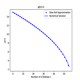
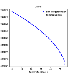
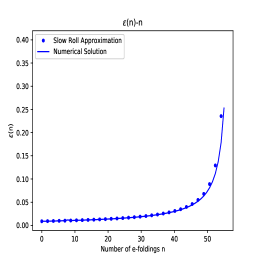
Figure 1: These graphs show the quantities $\psi(n)$, $\chi(n)$ and $\epsilon(n)$ for $U=\frac{1}{2}c^{2}\psi^{2}$ (with $c=7.126\times 10^{-6}$), starting from $\psi_{0}=15$ and $\psi_{0}^{\prime}=-\frac{2}{\psi_{0}}$. In each case numerical results for (12-13) are plotted as solid lines with the slow roll approximations (14) overlaid in large dots.

Because there is no perceptible difference we evolved the mode functions using the slow roll expressions (14).

We scale out the dimensions of the wave number and the $\phi$ mass, as well as taking the logarithm of the norm-squared of the mode functions,

$$\kappa\equiv\sqrt{8\pi G}\,k\quad,\quad\mu\equiv\sqrt{8\pi G}\,M\quad,\quad\mathcal{M}(n,\kappa,\mu)\equiv\ln\Biggl{[}\frac{|u(t,k,M)|^{2}}{\sqrt{8\pi G}}\Biggr{]}\;.$$ (15)

After some manipulations (for all the details when $M=0$, see [14, 15]) the mode equation and the Wronskian (9) can be combined to give a single, nonlinear equation for $\mathcal{M}(n,\kappa,\mu)$,

$$\mathcal{M}^{\prime\prime}+\frac{1}{2}{\mathcal{M}^{\prime}}^{2}+(3\!-\!\epsilon)\mathcal{M}^{\prime}+\frac{2\kappa^{2}e^{-2n}}{\chi^{2}}+\frac{2\mu^{2}}{\chi^{2}}-\frac{\exp[-6n-2\mathcal{M}]}{2\chi^{2}}=0\;.$$ (16)

In the far ultraviolet the physical wave number is much large than either the Hubble parameter or the mass and the mode function has the WKB form,

$$\frac{k}{a}\gg\Bigl{\{}H,M\Bigr{\}}\quad\Longrightarrow\quad u(t,k,M)\simeq\frac{1}{\sqrt{2ka^{2}(t)}}\,\exp\Biggl{[}-ik\!\!\int_{t_{i}}^{t}\!\!\frac{dt^{\prime}}{a(t^{\prime})}\Biggr{]}\;.$$ (17)

The WKB form (17) implies initial conditions for $\mathcal{M}(n,\kappa,\mu)\simeq-\ln(2\kappa)-2n$,

$$\mathcal{M}(0,\kappa,\mu)=\ln\Bigl{[}\frac{1}{2\kappa}\Bigr{]}\qquad,\qquad\mathcal{M}^{\prime}(0,\kappa,\mu)=-2\;.$$ (18)

2.2 Phases of $\mathcal{M}(n,\kappa,\mu)$

The amplitude function $\mathcal{M}(n,\kappa,\mu)$ exhibits a number of different behaviors which depend upon how the physical wave number $\kappa e^{-n}$ and the mass $\mu$ relate to the Hubble parameter $\chi(n)$. Two key wave numbers $n_{\kappa}$ and $n_{\mu}$ are defined by the relations,

$${\rm Horizon\ Crossing} \Longrightarrow \kappa\equiv e^{n_{\kappa}}\chi(n_{\kappa})\;,$$ (19)

$${\rm Mass\ Domination} \Longrightarrow \mu\equiv\frac{3}{2}\chi(n_{\mu})\;.$$ (20)

For some parameter choices Horizon Crossing and/or Mass Domination may occur before the start of inflation, or after its end (at $n_{e}$), and it may of course be that $n_{\mu}<n_{\kappa}$. However, under the “normal” assumption that $0<n_{\kappa}<n_{\mu}<n_{e}$ we distinguish three phases of evolution:

1. Ultraviolet, for $0\leq n\mathrel{\raise 1.29167pt\hbox{$<$\kern-7.5pt\lower 4.30554pt\hbox{$\sim$}}}n_{\kappa}+4$;

2. Steady Decline, for $n_{\kappa}+4\mathrel{\raise 1.29167pt\hbox{$<$\kern-7.5pt\lower 4.30554pt\hbox{$\sim$}}}n\leq n_{\mu}$; and

3. Oscillatory Decline, for $n_{\mu}\leq n\leq n_{e}$.

During the first phase $\mathcal{M}(n,\kappa,\mu)$ is well approximated by,

$$\mathcal{M}_{1}(n,\kappa,\mu)\equiv\ln\Biggl{[}\frac{1}{2\kappa e^{(D-2)n}}\!\times\!\frac{\pi}{2}\!\times\!z(n,\kappa)\!\times\!\Bigl{|}H^{(1)}_{\nu(n,\mu)}\Bigl{(}z(n,\kappa)\Bigr{)}\Bigr{|}^{2}\Biggr{]}\;,$$ (21)

where the argument $z(n,\kappa)$ and the index $\nu(n,\mu)$ are,

$$z(n,\kappa)\equiv\frac{\kappa e^{-n}}{[1\!-\!\epsilon(n)]\chi(n)}\;\;,\;\;\nu^{2}(n,\mu)\equiv\frac{1}{4}\Biggl{[}\frac{D\!-\!1\!-\!\epsilon(n)}{1\!-\!\epsilon(n)}\Biggr{]}^{2}-\Biggl{[}\frac{\mu}{[1\!-\!\epsilon(n)]\chi(n)}\Biggr{]}^{2}.$$ (22)

We shall always choose $\kappa$ so as to make $n_{\kappa}>0$, but we explore various choices of $\mu$. For relatively large masses, such as the cases of $\mu=10\chi(0)$ and $\mu=2\chi(0)$ which are shown in Figure 2, the system is mass dominated ($n_{\mu}<0$) from the beginning of inflation and expression (21) is an excellent approximation throughout inflation.

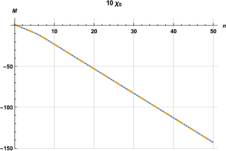
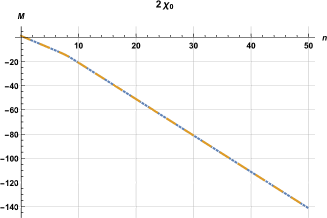
Figure 2: Both plots concern $\kappa=3800\chi_{0}$ (with $n_{\kappa}\simeq 8.32$) and $\omega^{2}(n,\mu)<0$ throughout inflation. The left hand graph compares the numerical result for $\mathcal{M}(n,\kappa,\mu)$ (in blue dots) with the approximation $\mathcal{M}_{1}(n,\kappa,\mu)$ (in long yellow dashes) given in expression (21) for $\mu=10\chi_{0}$. The right hand makes the same comparison for $\mu=2\chi_{0}$.

For smaller values of $\mu$ the onset of mass domination occurs after horizon crossing and the ultraviolet approximation (21) breaks down. This is shown for the case of $\mu=1.2\chi(0)$ in Figure 3.

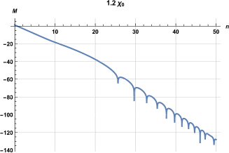
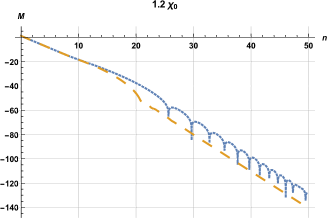
Figure 3: Both plots concern $\kappa=3800\chi_{0}$ (with $n_{\kappa}\simeq 8.32$) and $\mu=1.2\chi_{0}$ (with $n_{\mu}\simeq 20.25$). The left hand graph shows the numerical result for $\mathcal{M}(n,\kappa,\mu)$. The right hand graph compares this (in blue dots) with the approximation $\mathcal{M}_{1}(n,\kappa,\mu)$ (in long yellow dashes) given in expression (21).

In these cases it is useful to define differential frequency functions which are real on either side of mass domination,

$$\omega^{2}(n,\mu)\equiv\frac{9}{4}-\frac{\mu^{2}}{\chi^{2}(n)}\qquad,\qquad\Omega^{2}(n,\mu)\equiv\frac{\mu^{2}}{\chi^{2}(n)}-\frac{9}{4}\;.$$ (23)

If we define $n_{2}\equiv n_{\kappa}+4$, a good approximation for the second phase is,

$$\mathcal{M}_{2}(n,\kappa,\mu)=\mathcal{M}_{2}-3(n\!-\!n_{2})$$ (24)

$$+2\ln\Biggl{\{}\cosh\Biggl{[}\int_{n_{2}}^{n}\!\!\!dn^{\prime}\,\omega(n^{\prime},\mu)\Biggr{]}+\Bigl{(}\frac{\mathcal{M}_{2}^{\prime}\!+\!3}{2\omega(n_{2},\mu)}\Bigr{)}\sinh\Biggl{[}\int_{n_{2}}^{n}\!\!\!dn^{\prime}\,\omega(n^{\prime},\mu)\Biggr{]}\Biggr{\}}.\qquad$$

Defining $n_{3}\equiv n_{\mu}+4$ gives a good approximation for the third phase,

$$\mathcal{M}_{3}(n,\kappa,\mu)=\mathcal{M}_{3}-3(n\!-\!n_{3})$$ (25)

$$+2\ln\Biggl{\{}\Biggl{|}\cos\Biggl{[}\int_{n_{3}}^{n}\!\!\!dn^{\prime}\,\Omega(n^{\prime},\mu)\Biggr{]}+\Bigl{(}\frac{\mathcal{M}_{3}^{\prime}\!+\!3}{2\Omega(n_{3},\mu)}\Bigr{)}\sin\Biggl{[}\int_{n_{3}}^{n}\!\!\!dn^{\prime}\,\Omega(n^{\prime},\mu)\Biggr{]}\Biggr{|}\Biggr{\}}.\qquad$$

Figure 4 demonstrates the validity of these approximations for $\mu=1.2\chi(0)$.

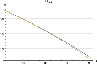
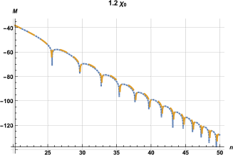
Figure 4: Like the previous figure, these plots deal concern $\kappa=3800\chi_{0}$ (with $n_{\kappa}\simeq 8.32$) and $\mu=1.2\chi_{0}$ (with $n_{\mu}\simeq 20.25$). The left hand graph compares the numerical result for $\mathcal{M}(n,\kappa,\mu)$ (in blue dots) with the “Steady Decline” approximation $M_{2}(n,\kappa,\mu)$ (in long yellow dashes) given in expression (24). The right hand graph compares $\mathcal{M}(n,\kappa,\mu)$ (in blue dots) with the “Oscillatory Decline” approximation $\mathcal{M}_{3}(n,\kappa,\mu)$ (in long yellow dashes) given in expression (25).

Making $\mu$ smaller postpones the onset of mass domination so late that the third phase comes near the end of inflation. Figure 5 shows this for $\mu=0.6\chi(0)$, which corresponds to $n_{\mu}\simeq 47.25$.

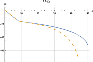
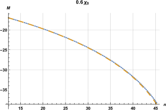
Figure 5: Both plots concern $\kappa=3800\chi_{0}$ (with $n_{\kappa}\simeq 8.32$) and $\mu=0.6\chi_{0}$ (with $n_{\mu}\simeq 47.25$). The left hand graph compares $\mathcal{M}(n,\kappa,\mu)$ (in blue dots) with the approximation $\mathcal{M}_{1}(n,\kappa,\mu)$ (in long yellow dashes) given in expression (21). The right hand graph compares $\mathcal{M}(n,\kappa,\mu)$ (in blue dots) with the approximation $M_{2}(n,\kappa,\mu)$ (in long yellow dashes) given in expression (24).

For very small values of $\mu$ the onset of mass domination never comes and only the first two phases are necessary. Figure 6 shows this for $\mu=0.1\chi(0)$, which would correspond to $n_{\mu}\simeq 56$ if slow roll inflation persisted that long.

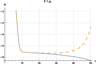
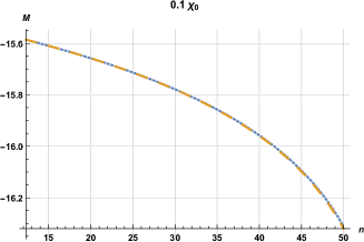
Figure 6: Both plots concern $\kappa=3800\chi_{0}$ (with $n_{\kappa}\simeq 8.32$) and $\mu=0.1\chi_{0}$ (with $n_{\mu}>50$). The left hand graph compares $\mathcal{M}(n,\kappa,\mu)$ (in blue dots) with the approximation $\mathcal{M}_{1}(n,\kappa,\mu)$ (in long yellow dashes) given in expression (21). The right hand graph compares $\mathcal{M}(n,\kappa,\mu)$ (in blue dots) with the approximation $M_{2}(n,\kappa,\mu)$ (in long yellow dashes) given in expression (24).

Because the coincidence limit (8) involves an integration over $\kappa=\sqrt{8\pi G}\times k$ it is crucial to determine how $\mathcal{M}(n,\kappa,\mu)$ depends on $\kappa$. This $\kappa$ dependence is manifest in the ultraviolet approximation (21), but there is no explicit $\kappa$ dependence in either of the later approximations (24) and (25). However, these approximations do depend on integration constants $\mathcal{M}_{2,3}$ and $\mathcal{M}_{2,3}^{\prime}$ which represent the values of $\mathcal{M}(n,\kappa,\mu)$ and its first derivative with respect to $n$ at $n_{2}=n_{\kappa}+4$ and $n_{3}=n_{\mu}+4$. It turns out that only $\mathcal{M}(n_{2,3},\kappa,\mu)$ depend significantly on $\kappa$. We can see this numerically by making plots of $\Delta\mathcal{M}(n,\mu)\equiv\mathcal{M}(n,\kappa_{1},\mu)-\mathcal{M}(n,\kappa_{2},\mu)$ for fixed wave numbers. Figure 7 gives three such plots for relatively small values of $\mu$ that would require more than just the ultraviolet phase. Because $\Delta\mathcal{M}(n,\mu)$ rapidly freezes in to a constant after horizon crossing we see that the two later phases inherit their $\kappa$ dependence from the ultraviolet phase,

$$\mathcal{M}_{2}(n,\kappa,\mu) = \mathcal{M}_{1}(n_{2},\kappa,\mu)+f_{2}(n,\mu)\;,$$ (26)

$$\mathcal{M}_{3}(n,\kappa,\mu) = \mathcal{M}_{1}(n_{2},\kappa,\mu)+f_{3}(n,\mu)\;.$$ (27)

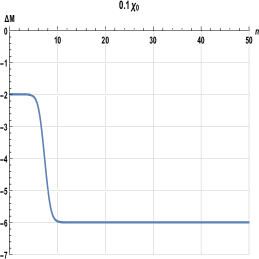
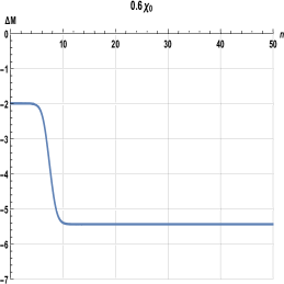
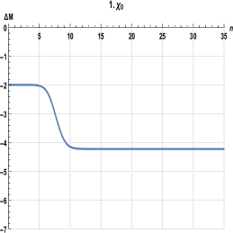
Figure 7: The left hand graph gives the difference of $\mathcal{M}(n,\kappa,\mu)$ between $\kappa=3800\chi_{0}$ (with $n_{\kappa}\simeq 8.32$) and $\kappa=520\chi_{0}$ (with $n_{\kappa}\simeq 6.31$) for $\mu=0.1\chi_{0}$. The middle and right hand graphs show the same difference for the cases of $\mu=0.6\chi_{0}$ and $\mu=\chi_{0}$, respectively.

Figure 8 gives three plots of $\Delta\mathcal{M}(n,\mu)$ for the intermediate values of $\mu$ over which the other phases drop out.

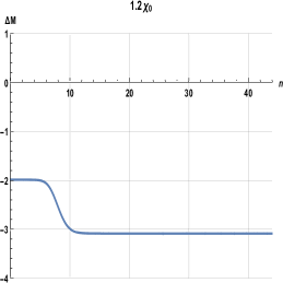
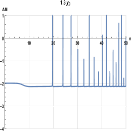
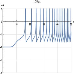
Figure 8: The left hand graph gives the difference of $\mathcal{M}(n,\kappa,\mu)$ between $\kappa=3800\chi_{0}$ (with $n_{\kappa}\simeq 8.32$) and $\kappa=520\chi_{0}$ (with $n_{\kappa}\simeq 6.31$) for $\mu=1.2\chi_{0}$. The middle and right hand graphs show the same difference for the cases of $\mu=1.3\chi_{0}$ and $\mu=1.35\chi_{0}$, respectively.

All three phases occur for $\mu=1.2\chi(0)$, and the difference is constant after horizon crossing. As $\mu$ is increased the difference exhibits a complex behavior, but one that is captured by the ultraviolet approximation (21). Figure 9 continues the progression to even larger values of $\mu$ for which the ultraviolet approximation suffices.

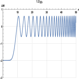
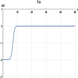
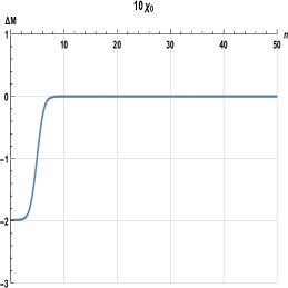
Figure 9: The left hand graph gives the difference of $\mathcal{M}(n,\kappa,\mu)$ between $\kappa=3800\chi_{0}$ (horizon crossing at $n_{\kappa}\simeq 8.32$) and $\kappa=520\chi_{0}$ (horizon crossing at $n_{\kappa}\simeq 6.31$) for $\mu=1.5\chi_{0}$. For this case the average post-horizon difference has become centered on zero while the fluctuations have become symmetric and more frequent yet. The middle and right hand graphs show the same difference for the cases of $\mu=2\chi_{0}$ and $\mu=10\chi_{0}$. The difference remains centered on zero with negligibly small oscillations.

2.3 Analytic Derivations

We had of course to set the spacetime dimension to $D=4$ in order to construct the various graphs of the previous sub-section. However, obtaining a reliable ultraviolet form requires generalizing the evolution equation (16) to general $D$,

$$\mathcal{M}^{\prime\prime}+\frac{1}{2}{\mathcal{M}^{\prime}}^{2}+(D\!-\!1\!-\!\epsilon)\mathcal{M}^{\prime}+\frac{2\kappa^{2}e^{-2n}}{\chi^{2}}+\frac{2\mu^{2}}{\chi^{2}}-\frac{\exp[-2(D-1)n-2\mathcal{M}]}{2\chi^{2}}=0\;.$$ (28)

Our initial motivation for the $\mathcal{M}_{1}(n,\kappa,\mu)$ approximation (21) was the Hubble effective potential [16] that would be relevant for constant $\epsilon(n)$ and the case where the mass parameter $\mu=\frac{h}{\sqrt{2}}\psi(n)$ is proportional to the Hubble parameter $\chi(n)$. To see that $\mathcal{M}_{1}(n,\kappa,\mu)$ is generally valid in the ultraviolet, we make the change of variables,

$$\mathcal{M}(n,\kappa,\mu)\equiv\mathcal{M}_{1}(n,\kappa,\mu)+g(n,\kappa,\mu)\equiv-\ln(2\kappa)-(D\!-\!2)n+\Delta\mathcal{M}_{1}+g\;.$$ (29)

Substituting (29) in (28) gives,

$$g^{\prime\prime}+\frac{{g^{\prime}}^{2}}{2}+\Bigl{(}1\!-\!\epsilon\!+\!\Delta\mathcal{M}_{1}^{\prime}\Bigr{)}g^{\prime}+\frac{2\kappa^{2}e^{-2\Delta\mathcal{M}_{1}}}{\chi^{2}e^{2n}}\Bigl{[}1-e^{-2g}\Bigr{]}=-\Delta\mathcal{M}_{1}^{\prime\prime}-\frac{{\Delta\mathcal{M}_{1}^{\prime}}^{2}}{2}$$ (30)

$$-(1\!-\!\epsilon)\Delta\mathcal{M}_{1}^{\prime}+2\Bigl{[}\Bigl{(}\frac{D}{2}\!-\!1\Bigr{)}\Bigl{(}\frac{D}{2}\!-\!\epsilon\Bigr{)}-\frac{\mu^{2}}{\chi^{2}}\Bigr{]}+\frac{2\kappa^{2}}{\chi^{2}e^{2n}}\Bigl{[}e^{-2\Delta\mathcal{M}_{1}}-1\Bigr{]}\;.\qquad$$

Now make the large $z$ expansion for $\Delta\mathcal{M}_{1}(n,\kappa,\mu)$,

$$e^{\Delta\mathcal{M}_{1}}=\frac{\pi}{2}z\Bigl{|}H^{(1)}_{\nu}(z)\Bigr{|}^{2}=1+\frac{(\nu^{2}\!-\!\frac{1}{4})}{2z^{2}}+\frac{3(\nu^{2}\!-\!\frac{1}{4})(\nu^{2}\!-\!\frac{9}{4})}{8z^{4}}+O\Bigl{(}\frac{1}{z^{6}}\Bigr{)}\;.$$ (31)

Substituting (31) into (30) and solving for $g(n,\kappa,\mu)$ in the ultraviolet regime of $\kappa\gg\chi(n)e^{n}$ implies the expansion,

$$g=\frac{1}{8}\Biggl{[}2\epsilon(5-3\epsilon)\frac{\mu^{2}}{\chi^{2}}+\Bigl{(}\frac{D}{2}-1\Bigr{)}\Bigl{[}(D+5-7\epsilon)\epsilon^{\prime}+\epsilon^{\prime\prime}\Bigr{]}\Biggr{]}\Bigl{(}\frac{\chi e^{n}}{\kappa}\Bigr{)}^{4}+O\Biggl{(}\Bigl{(}\frac{\chi e^{n}}{\kappa}\Bigr{)}^{6}\Biggr{)}.$$ (32)

This proves that the $\mathcal{M}_{1}(n,\kappa,\mu)$ approximation to $\mathcal{M}(n,\kappa,\mu)$ is valid until a few e-foldings before horizon crossing. (The graphical analysis of the previous subsection establishes that it is actually valid for some e-foldings after horizon crossing.) Combining expressions (8) and (32) also shows that the $\mathcal{M}_{1}(n,\kappa,\mu)$ approximation correctly captures the ultraviolet divergences of the coincident propagator and we can set $D=4$ in considering the later approximations.

The $\mathcal{M}_{2}(n,\kappa,\mu)$ approximation pertains after horizon crossing when the 4th and 6th terms of (16) have red-shifted into insignificance. Dropping these terms, and recalling the definition (23) of the frequency $\omega^{2}(n,\mu)$ we have,

$$\mathcal{M}^{\prime\prime}+\frac{1}{2}{\mathcal{M}^{\prime}}^{2}+(3\!-\!\epsilon)\mathcal{M}^{\prime}+\frac{9}{2}-2\omega^{2}\simeq 0\;.$$ (33)

Only derivatives of $\mathcal{M}$ appear in equation (33), and there is no explicit dependence on $\kappa$. Hence $\mathcal{M}^{\prime}$ can only depend on $\kappa$ through the initial condition at $n_{2}=n_{\kappa}+4$, and Figures 7-9 reveal no such dependence. We are therefore led to the change of variable,

$$\mathcal{M}^{\prime}(n,\mu)\simeq-3+2\omega(n,\mu)\tanh\Bigl{[}\alpha(n,\mu)\Bigr{]}$$ (34)

Substituting (34) in (33) leads to the relation,

$$2\omega\alpha^{\prime}{\rm sech}^{2}(\alpha)-2\omega^{2}{\rm sech}^{2}(\alpha)-\frac{9\epsilon}{2\omega}\tanh(\alpha)+3\epsilon\simeq 0\;.$$ (35)

Ignoring the last 2 terms, and imposing the correct initial condition at $n=n_{2}$ implies,

$$\mathcal{M}^{\prime}(n,\mu)\simeq-3+2\omega\tanh\Bigl{[}\alpha_{2}+\!\int_{n_{2}}^{n}\!\!\!dn^{\prime}\,\omega(n^{\prime},\mu)\Bigr{]}\;,\;\alpha_{2}=\tanh^{-1}\Bigl{[}\frac{\mathcal{M}_{2}^{\prime}\!+\!3}{2\omega_{2}}\Bigr{]}\;.$$ (36)

Integrating and using the $\kappa$-dependent initial condition gives,

$$\mathcal{M}(n,\kappa,\mu)\simeq\mathcal{M}_{2}-3(n\!-\!n_{2})+2\ln\Biggl{[}\frac{\cosh[\alpha_{2}+\int_{n_{2}}^{n}dn^{\prime}\omega(n^{\prime},\mu)]}{\cosh(\alpha_{2})}\Biggr{]}\;.$$ (37)

Breaking up the sum in the argument of the hyperbolic cosine leads to the $\mathcal{M}_{2}(n,\kappa,\mu)$ approximation (24). Because the term that was neglected in passing from (35) to (36) diverges when $\omega(n,\mu)$ vanishes, one expects the approximation to break down near $n=n_{\mu}$. This is just discernible in Figure 4.

The $\mathcal{M}_{3}(n,\kappa,\mu)$ approximation pertains after $\omega^{2}(n,\mu)=-\Omega^{2}(n,\mu)$ has changed from positive to negative. Although the 4th term in (16) continues to be negligible, the 6th term becomes significant over very brief intervals when $\mathcal{M}(n,\kappa,\mu)$ falls suddenly. Modeling this correctly is challenging because the intervals over which the 6th term matters are so short. The simplest approach turns out to be ignoring 6th term, and accounting for its brief impact with a judicious absolute value.

If $n>n_{\mu}$, and we continue to ignore the 4th and 6th terms in (16), the appropriate equation for $\mathcal{M}(n,\kappa,\mu)$ is,

$$\mathcal{M}^{\prime\prime}+\frac{1}{2}{\mathcal{M}^{\prime}}^{2}+(3\!-\!\epsilon)\mathcal{M}^{\prime}+\frac{9}{2}+2\Omega^{2}\simeq 0\;.$$ (38)

The appropriate substitution is,

$$\mathcal{M}^{\prime}(n,\mu)\simeq-3+2\Omega(n,\mu)\tan\Bigl{[}\beta(n,\mu)\Bigr{]}$$ (39)

Making this substitution brings equation (38) to the form,

$$2\Omega\beta^{\prime}\sec^{2}(\beta)+2\Omega^{2}\sec^{2}(\beta)+\frac{9\epsilon}{2\Omega}\tan(\beta)+3\epsilon\simeq 0\;.$$ (40)

If we ignore the final term then the solution is,

$$\mathcal{M}^{\prime}(n,\mu)\simeq-3+2\Omega\tan\Bigl{[}\beta_{3}-\!\int_{n_{3}}^{n}\!\!\!dn^{\prime}\,\Omega(n^{\prime},\mu)\Bigr{]}\;,\;\beta_{3}=\tan^{-1}\Bigl{[}\frac{\mathcal{M}_{3}^{\prime}\!+\!3}{2\Omega_{3}}\Bigr{]}\;.$$ (41)

Integrating this expression, and supplying the aforementioned absolute value gives,

$$\mathcal{M}(n,\kappa,\mu)\simeq\mathcal{M}_{3}-3(n\!-\!n_{3})+2\ln\Biggl{[}\Biggl{|}\frac{\cos[\beta_{3}-\int_{n_{3}}^{n}dn^{\prime}\Omega(n^{\prime},\mu)]}{\cos(\beta_{3})}\Biggr{|}\Biggr{]}\;.$$ (42)

Breaking up the argument of the cosine gives expression (25) for $\mathcal{M}_{3}(n,\kappa,\mu)$.

3 Computing the Inflaton Effective Potential

The point of developing approximate analytic forms for $\mathcal{M}(n,\kappa,\mu)$ like expressions (21), (24) and (25) is to compute the derivative of the effective potential (7) through the coincident propagator (8). That is the purpose of this section. We first decompose the integration into ultraviolet, for which expression (21) pertains, and infrared, for which expressions (24) and (25) apply. Only the ultraviolet part requires dimensional regularization, whereas the $\kappa$ dependence of the infrared part can be factored out, and expressed in terms of $\mathcal{M}_{1}(n,\kappa,\mu)$, using relations (26-27).

The graphical analysis of section 2.2 shows that a reasonable point for the transition between the $\mathcal{M}_{1}$ and the $\mathcal{M}_{2}$ approximations is about 4 e-foldings after horizon crossing. This corresponds to a wave number $K(n)$,

$$K(n)\equiv\frac{e^{n-4}\chi(n\!-\!4)}{\sqrt{8\pi G}}\quad\Longrightarrow\quad\begin{cases}{\rm UV:}&k>K(n)\\ {\rm IR:}&k<K(n)\end{cases}\;.$$ (43)

This distinction allows us to approximate the coincident propagator (8) as,

$$i\Delta(x;x) = \frac{2\sqrt{8\pi G}}{(4\pi)^{\frac{D-1}{2}}\Gamma(\frac{D-1}{2})}\int_{0}^{\infty}\!\!\!\!dk\,k^{D-2}\,e^{\mathcal{M}(n,\kappa,\mu)}\;,$$ (45)

$$\simeq \frac{2\sqrt{8\pi G}}{(4\pi)^{\frac{D-1}{2}}\Gamma(\frac{D-1}{2})}\int_{0}^{\infty}\!\!\!\!dk\,k^{D-2}\,e^{\mathcal{M}_{1}(n,\kappa,\mu)}$$

$$\hskip 56.9055pt+\frac{\sqrt{8\pi G}}{2\pi^{2}}\int_{0}^{K(n)}\!\!\!\!dk\,k^{2}\Biggl{[}e^{\mathcal{M}_{2,3}(n,\kappa,\mu)}-e^{\mathcal{M}_{1}(n,\kappa,\mu)}\Biggr{]}\;.\qquad$$

We define the first term on the right hand side of (45) as $i\Delta_{1}(x;x)$, and the second term as $i\Delta_{\rm IR}(x;x)$.

We compute $i\Delta_{1}(x;x)$ using expression (21) with integral 6.574 #2 of [17],

$$i\Delta_{1}(x;x)=\frac{[(1\!-\!\epsilon)H]^{D-2}}{(4\pi)^{\frac{D}{2}}}\times\frac{\Gamma(\frac{D-1}{2}\!+\!\nu)\Gamma(\frac{D-1}{2}\!-\!\nu)}{\Gamma(\frac{1}{2}\!+\!\nu)\Gamma(\frac{1}{2}\!-\!\nu)}\times\Gamma\Bigl{(}1\!-\!\frac{D}{2}\Bigr{)}\;,$$ (46)

where $\nu(n,\mu)$ is given in expression (22). Writing $D=4-\delta$ and expanding key terms gives,

$$i\Delta_{1}(x;x)=\frac{[(1\!-\!\epsilon)H]^{D-2}}{(4\pi)^{\frac{D}{2}}}\Bigl{[}\Bigr{(}\frac{D\!-\!3}{2}\Bigr{)}^{2}-\nu^{2}\Bigr{]}$$ (48)

$$\hskip 85.35826pt\times-\frac{2}{\delta}\Biggl{\{}1-\Bigl{[}\psi\Bigl{(}\frac{1}{2}+\nu\Bigr{)}+\psi\Bigl{(}\frac{1}{2}-\nu\Bigr{)}\Bigr{]}\frac{\delta}{2}+O(\delta^{2})\Biggr{\}},\qquad$$

$$\hskip 14.22636pt=\frac{[(1\!-\!\epsilon)H]^{D-4}}{(4\pi)^{\frac{D}{2}}}\Biggl{\{}-\frac{1}{4}\Bigl{(}\frac{D\!-\!2}{D\!-\!1}\Bigr{)}R+M^{2}-\frac{\delta}{2}\Bigl{(}1\!-\!\frac{\delta}{2}\Bigr{)}(1\!-\!\epsilon)^{2}H^{2}\Biggr{\}}$$

$$\hskip 113.81102pt\times\Biggl{\{}-\frac{2}{\delta}+\psi\Bigl{(}\frac{1}{2}+\nu\Bigr{)}+\psi\Bigl{(}\frac{1}{2}-\nu\Bigr{)}+O(\delta)\Biggr{\}},\qquad$$

where $R=(D-1)(\frac{D}{2}-2\epsilon)H^{2}$ is the Ricci scalar. Comparison with expression (7) reveals that the conformal and quartic counterterms are,

$$\delta\xi = \frac{h^{2}s^{D-4}}{(4\pi)^{\frac{D}{2}}}\times\frac{(D\!-\!2)}{4(D\!-\!1)(D\!-\!4)}+\frac{h^{2}\delta\xi_{\rm fin}}{32\pi^{2}}\;,$$ (49)

$$\delta\lambda = \frac{h^{4}s^{D-4}}{(4\pi)^{\frac{D}{2}}}\times-\frac{3}{D\!-\!4}+\frac{h^{4}\delta\lambda_{\rm fin}}{64\pi^{2}}\;,$$ (50)

where $s$ is the mass scale of dimensional regularization and $\delta\xi_{\rm fin}$ and $\delta\lambda_{\rm fin}$ represent arbitrary finite renormalizations. Substituting expressions (48-50) into (7) and taking the unregulated limit gives the $\mathcal{M}_{1}(n,\kappa,\mu)$ contribution to the effective potential,

$$\Bigl{(}\frac{\partial V_{\rm eff}}{\partial\varphi}\Bigr{)}_{1}=\frac{h^{2}\varphi}{32\pi^{2}}\Biggl{\{}(1\!-\!\epsilon)^{2}H^{2}+\delta\xi_{\rm fin}R+\frac{1}{12}\delta\lambda_{\rm fin}h^{2}\varphi^{2}$$ (51)

$$\hskip 14.22636pt+\Bigl{[}-\frac{1}{6}R+\frac{1}{2}h^{2}\varphi^{2}\Bigr{]}\Biggl{[}\psi\Bigl{(}\frac{1}{2}\!+\!\nu\Bigr{)}+\psi\Bigl{(}\frac{1}{2}\!-\!\nu\Bigr{)}+\ln\Bigl{[}\frac{(1\!-\!\epsilon)^{2}H^{2}}{s^{2}}\Bigr{]}\Biggr{]}\Biggr{\}},\qquad$$

where the unregulated limit of the index is,

$$\nu=\frac{\sqrt{(\frac{3-\epsilon}{2})^{2}-z}}{1\!-\!\epsilon}\qquad,\qquad z\equiv\frac{h^{2}\varphi^{2}}{2H^{2}}\;.$$ (52)

Integrating with respect to $\varphi$ allows us to express the $\mathcal{M}_{1}$ contribution in terms of the instantaneous values of $H$, $\epsilon$ and $z$,

$$\Bigl{(}V_{\rm eff}\Bigr{)}_{1}=$$ (53)

$$\frac{H^{4}}{32\pi^{2}}\Biggl{\{}(1\!-\!\epsilon)^{2}z+6\delta\xi_{\rm fin}(2\!-\!\epsilon)z+\frac{\delta\lambda_{\rm fin}z^{2}}{12}-\Bigl{[}(2\!-\!\epsilon)z-\frac{z^{2}}{2}\Bigr{]}\ln\Bigl{[}\frac{(1\!-\!\epsilon)^{2}H^{2}}{s^{2}}\Bigr{]}$$

$$+\!\!\int_{0}^{z}\!\!\!dx\,(-2\!+\!\epsilon\!+\!x)\Biggl{[}\psi\Biggl{(}\!\frac{1}{2}+\frac{\sqrt{(\frac{3-\epsilon}{2})^{2}-x}}{1\!-\!\epsilon}\Biggr{)}\!+\psi\Biggl{(}\!\frac{1}{2}-\frac{\sqrt{(\frac{3-\epsilon}{2})^{2}-x}}{1\!-\!\epsilon}\Biggr{)}\Biggr{]}\!\Biggr{\}}.\qquad$$

It remains to evaluate expression (45) for $i\Delta_{\rm IR}(x;x)$. Note from relations (26-27), and the slow roll approximation for the post-horizon amplitude, that dependence on the mass parameter $\mu$ factors out of the integration over wave number $k$,

$$i\Delta_{\rm IR}(x;x) = \frac{\sqrt{8\pi G}}{2\pi^{2}}\int_{0}^{K(n)}\!\!\!\!dk\,k^{2}e^{\mathcal{M}_{1}(n_{\kappa}+4,\kappa,\mu)}\times\Bigl{\{}e^{f_{2,3}(n,\mu)}-e^{f_{1}(n,\kappa,\mu)}\Bigr{\}}\;,\qquad$$ (54)

$$\simeq \frac{1}{4\pi^{2}}\int_{0}^{K(n)}\!\!\frac{dk}{k}H^{2}(t_{k})\times\Bigl{\{}e^{f_{2,3}(n,\mu)}-e^{f_{1}(n,\kappa,\mu)}\Bigr{\}}\;,$$ (55)

where $f_{i}\equiv\mathcal{M}_{i}(n,\kappa,\mu)-\mathcal{M}_{1}(n_{\kappa}\!+\!4,\kappa,\mu)$. Now change variables from $k$ to $n_{\kappa}$ using $dk/k=(1-\epsilon)dn_{\kappa}$,

$$i\Delta_{\rm IR}(x;x)\simeq\frac{1}{4\pi^{2}}\int_{0}^{n-4}\!\!\!\!dn_{\kappa}\frac{[1\!-\!\epsilon(n_{\kappa})]\chi^{2}(n_{\kappa})}{8\pi G}\times\Bigl{\{}e^{f_{2,3}(n,\mu)}-e^{f_{1}(n,e^{n_{\kappa}}\chi(n_{\kappa}),\mu)}\Bigr{\}}\;.$$ (56)

Note the distinction between the integration over $n_{\kappa}$ and the multiplicative factor which depends on the local e-folding $n$. This means that $i\Delta_{\rm IR}(x;x)$ is not even a local function of the inflationary geometry. The factors of $e^{f_{2}(n,\mu)}$ and $e^{f_{3}(n,\mu)}$ also depend nonlocally on the geometry,

$$e^{f_{2}(n,\mu)} = e^{-3(n-n_{2})}\frac{\cosh^{2}[\alpha_{2}+\int_{n_{2}}^{n}dn^{\prime}\omega(n^{\prime},\mu)]}{\cosh^{2}(\alpha_{2})}\;,$$ (57)

$$e^{f_{3}(n,\mu)} = e^{f_{2}(n,\mu)}\times\frac{\cos^{2}[\beta_{3}-\int_{n_{3}}^{n}dn^{\prime}\Omega(n^{\prime},\mu)]}{\cos^{2}(\beta_{3})}\;.$$ (58)

Expression (56) gives the nonlocal contribution to the coincident propagator. To find the corresponding contribution to the effective potential one substitutes this in expression (7) and then integrates with respect to the inflaton field $\varphi$, not excepting the dependence on $\mu^{2}=8\pi G\times\frac{1}{2}h^{2}\varphi^{2}$. Note that although the result depends nonlocally on the geometry, it is local in the inflaton. Obtaining an explicit result is not possible owing to the complicated $\mu$-dependence of the functions $f_{2}(n,\mu)$ and $f_{3}(n,\mu)$, however, under the (expected) assumption that expressions (57-58) are small, the result is,

$$\Bigl{(}V_{\rm eff}\Bigr{)}_{IR}\simeq\frac{1}{4}h^{2}\varphi^{2}\times-\frac{1}{4\pi^{2}}\int_{0}^{n-4}\!\!\!\!dn^{\prime}[1\!-\!\epsilon(n^{\prime})]H^{2}(n^{\prime})\;.$$ (59)

We recognize (59) as a negative contribution to the inflaton mass-squared. How significant it is depends on the classical model of inflation. For the quadratic potential we have been assuming, with our initial conditions, the correction (59) would subtract off a fraction $\frac{75h^{2}}{16\pi^{2}}\simeq\frac{1}{2}h^{2}$ of the inflaton mass. This could make significant changes to the inflaton’s evolution, but these could be compensated by increasing the bare mass. The consequences for the geometry are more difficult to estimate but two features are obvious:

• Nonlocal corrections can contaminate late time physics, when scales should be small, with information from very early times, when scales were large; and

• Nonlocal corrections cannot be subtracted off using local actions.

4 Modified Friedmann Equations

The purpose of this section is to derive the nontrivial equations for a gravitational Lagrangian whose specialization to the geometry of inflation (2) takes the form $L(a,\dot{a},\ddot{a})=a^{3}f(H,\epsilon)$. If we knew the Lagrangian for a general metric then first varying with respect to $g^{\mu\nu}$ and afterwards specializing to (2) would give two nontrivial equations, one from the variation with respect to $g^{ij}$ and the other from the variation with respect to $g^{00}$. However, specializing the geometry first gives only one equation. The famous theorem of Palais [18] assures us that this equation is correct, and we know from the fact that $g_{ij}=a^{2}\delta_{ij}$ that this equation is proportional to the variation with respect to $g^{ij}$. We begin by deriving this equation, then we reconstruct the $g^{00}$ equation using conservation. The section closes by checking that our results agree for the special cases of no dependence upon $\epsilon$ and also $F(R)$ models.

For a Lagrangian of the form $L(a,\dot{a},\ddot{a})=a^{3}f(H,\epsilon)$ the Euler-Lagrange equation is,

$$\frac{\partial L}{\partial a}-\frac{d}{dt}\Bigl{(}\frac{\partial L}{\partial\dot{a}}\Bigr{)}+\frac{d^{2}}{dt^{2}}\Bigl{(}\frac{\partial L}{\partial\ddot{a}}\Bigr{)}=a^{2}\Bigl{[}3f-H\frac{\partial f}{\partial H}-(1\!-\!\epsilon)\frac{\partial f}{\partial\epsilon}\Bigr{]}$$ (61)

$$\hskip 71.13188pt-\frac{d}{dt}\Biggl{\{}a^{2}\Bigl{[}\frac{\partial f}{\partial H}+\frac{2(1\!-\!\epsilon)}{H}\frac{\partial f}{\partial\epsilon}\Bigr{]}\Biggr{\}}+\frac{d^{2}}{dt^{2}}\Biggl{\{}a^{2}\Bigl{[}-\frac{1}{H^{2}}\frac{\partial f}{\partial\epsilon}\Bigr{]}\Biggr{\}},\quad$$

$$=a^{2}\Biggl{[}3f\!-\!\Bigl{(}\frac{d}{dt}\!+\!3H\Bigr{)}\frac{\partial f}{\partial H}\!-\!3(3\!+\!\epsilon)\frac{\partial f}{\partial\epsilon}\!-\!2(3\!+\!\epsilon)\frac{1}{H}\frac{d}{dt}\frac{\partial f}{\partial\epsilon}\!-\!\frac{1}{H^{2}}\frac{d^{2}}{dt^{2}}\frac{\partial f}{\partial\epsilon}\Biggr{]}.\quad$$

Because $g_{ij}=a^{2}\delta_{ij}$ for the geometry (2) we recognize the $g^{ij}$ equation as,

$$f\!-\!\Bigl{(}\frac{1}{3}\frac{d}{dt}\!+\!H\Bigr{)}\frac{\partial f}{\partial H}\!-\!(3\!+\!\epsilon)\frac{\partial f}{\partial\epsilon}\!-\!\Bigl{(}2\!+\!\frac{2}{3}\epsilon\Bigr{)}\frac{1}{H}\frac{d}{dt}\frac{\partial f}{\partial\epsilon}\!-\!\frac{1}{3H^{2}}\frac{d^{2}}{dt^{2}}\frac{\partial f}{\partial\epsilon}=0\;.$$ (62)

The conservation of stress-energy implies that (62) and the missing $g^{00}$ equation obey,

$$3H\Biggl{\{}\Bigl{(}g^{ij}\;{\rm Eqn}\Bigr{)}+\Bigl{(}g^{00}\;{\rm Eqn}\Bigr{)}\Biggr{\}}=\frac{d}{dt}\Bigl{(}g^{00}\;{\rm Eqn}\Bigr{)}\;.$$ (63)

We also want the $g^{00}$ equation to contain one fewer time derivative than (62). A little thought reveals the solution to be,

$$-f+H\frac{\partial f}{\partial H}+\Bigl{[}3\!+\!\epsilon+\frac{1}{H}\frac{d}{dt}\Bigr{]}\frac{\partial f}{\partial\epsilon}=0\;.$$ (64)

Relations (64) and (62) are the desired generalizations of the first and second Friedmann equations, respectively.

Relations (64) and (62) obey two important correspondence limits. The first comes from assuming that there is no dependence on $\epsilon$, as was considered in a previous study [10]. When $\frac{\partial f}{\partial\epsilon}=0$ our Friedmann equations agree with relations (15) and (14) from that study. The second limit is relevant to $F(R)$ models,

$$f(H,\epsilon)\longrightarrow F\Bigl{(}(12\!-\!6\epsilon)H^{2}\Bigr{)}\;.$$ (65)

In that limit we have,

$$\frac{\partial f}{\partial H}\longrightarrow(24\!-\!12\epsilon)H\!\times\!F^{\prime}\qquad,\qquad\frac{\partial f}{\partial\epsilon}\longrightarrow-6H^{2}\!\times\!F^{\prime}\;.$$ (66)

Substituting these relations into our first Friedmann equation (64) gives,

$$\Bigl{(}{\rm Eqn\ \ref{Feqn1}}\Bigr{)}\longrightarrow-F(R)+6(1\!-\!\epsilon)H^{2}F^{\prime}(R)-6H\frac{d}{dt}F^{\prime}(R)=0\;.$$ (67)

With (66) our second Friedmann equation (62) becomes,

$$\Bigl{(}{\rm Eqn\ \ref{Feqn2}}\Bigr{)}\longrightarrow+F(R)-(6\!-\!2\epsilon)H^{2}F^{\prime}(R)+4H\frac{d}{dt}F^{\prime}(R)+2\frac{d^{2}}{dt^{2}}F^{\prime}(R)=0\;.$$ (68)

Relations (67-68) can be recognized as the specialization the $F(R)$ field equations to the geometry (2) of inflation.

The Friedmann equation of general relativity ($3H^{2}=8\pi G\rho$) involves only first derivatives of the scale factor $a(t)$, whereas our generalization (64) involves three derivatives. Similarly, the $g_{ij}$ equation of general relativity ($-2\dot{H}-3H^{2}=8\pi Gp$) involves second derivatives of $a(t)$, whereas our generalization (62) involves four time derivatives. Classical theories that involve higher time derivatives have new degrees of freedom which are typically kinetically unstable [12]. The unique local and invariant modification of general relativity that avoids kinetic instabilities is $F(R)$ models (65) [12], but a glance at expression (53) reveals that the myriad factors of $H$ and $\epsilon$ in the effective potential are not limited to the combination $R=6(2-\epsilon)H^{2}$. This sounds like a major problem, and it probably is, but not in the direct way one might think. Quantum corrections to the effective action are typically not even local, and yet they introduce no new degrees of freedom nor any essential instability. The right way to understand these higher derivative or nonlocal quantum corrections is as perturbations to the existing solutions of the classical, lower-derivative theory [19]. Quantum corrections introduce no new degrees of freedom, they simply distort the evolution of the classical degrees of freedom. Unfortunately, the distortion from cosmological Coleman-Weinberg potentials is typically too large because these corrections are not Planck-suppressed. To avoid large distortions one must subtract most of the cosmological Coleman-Weinberg potential using a classical modification of the original model. Because the subtraction has the status of a modification to the classical action, it can induce new degrees of freedom and instabilities. A recent study of subtractions involving functions of the inflaton and the Ricci scalar reveals that the higher derivative degrees of freedom cause inflation to end after an infinitesimal number of e-foldings [11].

5 Epilogue

We have developed an analytic approximation for the logarithm of the amplitude of the norm-squared mode function for a massive, minimally coupled scalar in the presence of an arbitrary inflating background. Our result takes the form of a sequence of approximate forms that apply when the physical wave number dominates the Hubble parameter — expression (21) — when the Hubble parameter dominates the physical wave number and the mass — expression (24) — and after the mass dominates the Hubble parameter — expression (25). Section 2.2 contains many graphs which demonstrate the validity of these approximations for inflation with a quadratic potential, and section 2.3 gives analytic derivations which should apply for general models.

The quadratic dimensionless potential $U(\psi)=\frac{1}{2}c^{2}\psi^{2}$ was chosen for our detailed studies because the slow roll approximations (14) give simple, analytic expressions for the dimensionless Hubble parameter $\chi(n)$ and the first slow roll parameter $\epsilon(n)$. With the choice of $c\simeq 7.1\times 10^{-6}$ this model is consistent with observations of the scalar amplitude and the scalar spectral index [1]. However, the model is excluded by its high prediction of $r\simeq 0.14$ for the tensor-to-scalar ratio [1]. It is worth briefly considering how our analysis applies to the plateau potentials that are currently permitted by the data. Perhaps the simplest of these is the Einstein-frame version of the model proposed by Starobinsky [20], whose dimensionless potential is [21],

$$U(\psi)=\frac{3}{4}M^{2}\Bigl{(}1-e^{-\sqrt{\frac{2}{3}}\,\psi}\Bigr{)}^{2}\qquad,\qquad M^{2}=1.3\times 10^{-5}\;.$$ (69)

Starting from $\psi_{0}=5.3$ gives a little over 50 e-foldings of inflation, and the model is consistent with observations. A glance at Figure 10 reveals how this is achieved: the dimensionless Hubble parameter $\chi(n)$ is almost constant, implying a very small value of the first slow roll parameter $\epsilon(n)$.

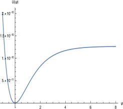
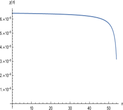
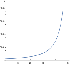
Figure 10: These graphs show the Starobinsky potential $U(\psi)$ of expression (69), as well as the dimensionless Hubble parameter $\chi(n)$ and the first slow roll parameter $\epsilon(n)$ for inflation starting from $\psi_{0}=5.3$.

All our approximations continue to apply to this model, but the extreme flatness of $\chi(n)$ restricts the range of dimensionless mass parameters $\mu$ for which $\chi(n)$ can make the transition from being greater than $\frac{2}{3}\mu$ to being less that is associated with the $\mathcal{M}_{3}(n,\kappa,\mu)$ approximation (25). This is shown in Figure 11, which compares $\mathcal{M}(n,\kappa,\mu)$ with the $\mathcal{M}_{1}(n,\kappa,\mu)$ approximation (21) for three different values of $\mu$.

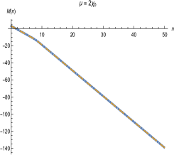
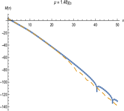
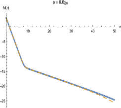
Figure 11: These graphs compare the numerical solution of $\mathcal{M}(n,\kappa,\mu)$ (in blue dots) with the $\mathcal{M}_{1}(n,\kappa,\mu)$ approximation (in long yellow dashes) for inflation driven by the Starobinsky potential (69).

When $\mu=2\chi_{0}$ the dimensionless Hubble parameter is always less than $\frac{2}{3}\mu$ and the $\mathcal{M}_{1}(n,\kappa,\mu)$ approximation remains valid throughout inflation. Indeed, the graph for $\mu=2\chi_{0}$ is almost identical to the $\mu=2\chi_{0}$ graph for the quadratic model in Figure 2. Only when $\mu$ is slightly smaller than $\frac{3}{2}\chi_{0}$ can the transition be made to happen during inflation, as it does for the case of $\mu=1.48\chi_{0}$ in Figure 11. For this case the transition comes at $n_{\mu}\simeq 28.2$, and one can see from the graph that all three approximations are required. When $\mu$ becomes even slightly smaller the transition does not occur during inflation. For example, the case of $\mu=1.4\chi_{0}$ corresponds to $n_{\mu}\simeq 46.7$. For smaller values of $\mu$ the $\mathcal{M}_{1}(n,\kappa,\mu)$ approximation applies until somewhat after horizon crossing, after which the $\mathcal{M}_{2}(n,\kappa,\mu)$ approximation pertains. The case of $\mu=0.6\chi_{0}$ is given in Figure 11, and is similar to what Figure 5 shows for the quadratic model with the same value of $\mu$.

The primary motivation for this work was to determine how Coleman-Weinberg corrections to the inflaton potential depend on the geometry of inflation so that previous studies of their effects [10, 11] can be extended. Our result consists of a local part (53) that depends on the instantaneous values of $H$ and $\epsilon$, and a nonlocal part — derived from integrating $\frac{1}{2}h^{2}\varphi$ times expression (56) — that depends on the past geometry. We emphasize that these approximations are independent of the classical potential and depend only on the coupling (6) between the inflaton $\varphi$ and the scalar $\phi$. It is also significant that the various factors of $H$ and $\epsilon$ in the local part (53) are not restricted to the Ricci scalar $R=6(2-\epsilon)H^{2}$. This fact, and the existence of the nonlocal correction, were predicted on the basis of indirect arguments [9].

Because the most general, stable subtraction is a local function of $\varphi$ and $R$, complete subtraction is impossible and there can no longer be any doubt that cosmological Coleman-Weinberg potentials make significant changes to inflation. Determining what those changes are requires understanding how cosmological Coelman-Weinberg potentials modify the Friedmann equations. Generalizing the Friedmann equations to include the nonlocal contributions is challenging, but those contributions should be small because the mass term suppresses the amplitude at late times. The Friedmann equations appropriate to the local part (53) are (64) and (62).

Although we have considered cosmological Coleman-Weinberg potentials from coupling the inflaton to a scalar (6), our results should be easily extendable to more general couplings. So we will finally be able to extend the old de Sitter results to a general inflationary background for the case of an inflaton which is Yukawa-coupled to fermions [22, 23], and to a charged inflaton which is coupled to a vector boson [24, 25]. It is also worth pointing out that our approximation seems to be valid even for a moderately time dependent inflaton $\varphi_{0}(t)$. Indeed, the crucial $\mathcal{M}_{1}$ approximation (21) was originally motivated by the exact result for $\phi_{0}(t)\propto H(t)$ [16] for constant $\epsilon$.

Finally, we should mention the impact of cosmological Coleman-Weinberg potentials on primordial perturbations, which are the principal observable from inflation. Slow roll approximations for the scalar and tensor power spectra can be expressed as functions of the e-folding $n$ at which a perturbation experiences horizon crossing, in terms of the dimensionless Hubble parameter $\chi(n)$ and first slow roll parameter $\epsilon(n)$,

$$\Delta^{2}_{\mathcal{R}}(n)\simeq\frac{1}{8\pi^{2}}\!\times\!\frac{\chi^{2}(n)}{\epsilon(n)}\qquad,\qquad\Delta^{2}_{h}(n)\simeq\frac{1}{8\pi^{2}}\!\times\!16\chi^{2}(n)\;.$$ (70)

The analogous slow roll approximations for the scalar spectral index and the tensor-to-scalar ratio are,

$$1-n_{s}(n)\simeq 2\epsilon(n)+\frac{\epsilon^{\prime}(n)}{\epsilon(n)}\qquad,\qquad r(n)\simeq 16\epsilon(n)\;.$$ (71)

Arbitrarily accurate analytic approximations are available [27, 28] if greater precision is required, and the same is true for the tri-spectrum of non-Gaussianity [29].

Cosmological Coleman-Weinberg potentials change the predictions (70-71) by changing the numerical values of the geometrical parameters $\chi(n)$ and $\epsilon(n)$ through the modified Friedmann equations (64) and (62). Unless the coupling constant $h$ is made so small as to preclude efficient re-heating, the changes induced by our result (53) are far too large for any viable classical model of inflation. This has long been apparent from the flat space limit $(V_{\rm eff})_{1}\rightarrow\frac{h^{4}\varphi^{4}}{256\pi^{2}}\ln(\frac{h^{2}\varphi^{2}}{2s^{2}})$ [7], which is also the large field limit. That term could be subtracted off, but the remainder after even the best possible subtractions still causes inflation to end too quickly [10, 11]. A more promising approach seems to be arranging cancellations between the positive cosmological Coleman-Weinberg potentials induced by coupling to bosonic fields and the negative potentials induced by coupling to fermions [30], although no solution has been devised yet.

If an acceptable cancellation can be found it will also be necessary to check for changes to the functional forms (70-71) of the inflationary observables. Because these results derive from the linearized field equations of perturbations about the cosmological background, they might show significant changes even if the Bose-Fermi cancellation kept changes to the background small. One would need to compute the 1PI (one-particle-irreducible) 2-point functions for the inflaton and for the metric in an inflationary background. Those computations would be challenging but it is encouraging that the results for de Sitter background have been obtained [31, 32, 33].

Acknowledgements

We are grateful for discussions and correspondence with A. Starobinsky. This work was partially supported by Taiwan MOST grant 107-2119-M-006-014 and 108-2112-M-006-004; by the European Union’s Seventh Framework Programme (FP7-REGPOT-2012-2013-1) under grant agreement number 316165; by the European Union’s Horizon 2020 Programme under grant agreement 669288-SM-GRAV-ERC-2014-ADG; by NSF grants PHY-1806218 and PHY-1912484; and by the Institute for Fundamental Theory at the University of Florida.

References

- [1] N. Aghanim et al. [Planck Collaboration], arXiv:1807.06209 [astro-ph.CO].
- [2] A. Ijjas, P. J. Steinhardt and A. Loeb, Phys. Lett. B 723, 261 (2013) doi:10.1016/j.physletb.2013.05.023 [arXiv:1304.2785 [astro-ph.CO]].
- [3] A. H. Guth, D. I. Kaiser and Y. Nomura, Phys. Lett. B 733, 112 (2014) doi:10.1016/j.physletb.2014.03.020 [arXiv:1312.7619 [astro-ph.CO]].
- [4] A. Linde, doi:10.1093/acprof:oso/9780198728856.003.0006 arXiv:1402.0526 [hep-th].
- [5] A. H. Guth et al. [33 co-authors], “A Cosmic Controversy,” (Letter to the Editor), Scientific American (May 10, 2017).
- [6] A. Ijjas, P. J. Steinhardt and A. Loeb, Phys. Lett. B 736, 142 (2014) doi:10.1016/j.physletb.2014.07.012 [arXiv:1402.6980 [astro-ph.CO]].
- [7] S. R. Coleman and E. J. Weinberg, Phys. Rev. D 7, 1888 (1973). doi:10.1103/PhysRevD.7.1888
- [8] D. R. Green, Phys. Rev. D 76, 103504 (2007) doi:10.1103/PhysRevD.76.103504 [arXiv:0707.3832 [hep-th]].
- [9] S. P. Miao and R. P. Woodard, JCAP 1509, no. 09, 022 (2015) doi:10.1088/1475-7516/2015/09/022, 10.1088/1475-7516/2015/9/022 [arXiv:1506.07306 [astro-ph.CO]].
- [10] J. H. Liao, S. P. Miao and R. P. Woodard, Phys. Rev. D 99, no. 10, 103522 (2019) doi:10.1103/PhysRevD.99.103522 [arXiv:1806.02533 [gr-qc]].
- [11] S. P. Miao, S. Park and R. P. Woodard, Phys. Rev. D 100, no.10, 103503 (2019) doi:10.1103/PhysRevD.100.103503 [arXiv:1908.05558 [gr-qc]].
- [12] R. P. Woodard, Lect. Notes Phys. 720, 403 (2007) doi:10.1007/978-3-540-71013-4_14 [astro-ph/0601672].
- [13] F. Finelli, G. Marozzi, A. A. Starobinsky, G. P. Vacca and G. Venturi, Phys. Rev. D 79, 044007 (2009) doi:10.1103/PhysRevD.79.044007 [arXiv:0808.1786 [hep-th]].
- [14] M. G. Romania, N. C. Tsamis and R. P. Woodard, JCAP 1208, 029 (2012) doi:10.1088/1475-7516/2012/08/029 [arXiv:1207.3227 [astro-ph.CO]].
- [15] D. J. Brooker, N. C. Tsamis and R. P. Woodard, Phys. Rev. D 93, no. 4, 043503 (2016) doi:10.1103/PhysRevD.93.043503 [arXiv:1507.07452 [astro-ph.CO]].
- [16] T. M. Janssen, S. P. Miao, T. Prokopec and R. P. Woodard, JCAP 0905, 003 (2009) doi:10.1088/1475-7516/2009/05/003 [arXiv:0904.1151 [gr-qc]].
- [17] I. S. Gradshteyn and I. M. Ryzhik, “Table of Integrals, Series and Products, 4th Edition,” (New York, Academic Press, 1965).
- [18] R. S. Palais, Commun. Math. Phys. 69, no. 1, 19 (1979). doi:10.1007/BF01941322
- [19] J. Z. Simon, Phys. Rev. D 41, 3720 (1990). doi:10.1103/PhysRevD.41.3720
- [20] A. A. Starobinsky, Adv. Ser. Astrophys. Cosmol. 3, 130-133 (1987) doi:10.1016/0370-2693(80)90670-X
- [21] D. J. Brooker, S. D. Odintsov and R. P. Woodard, Nucl. Phys. B 911, 318-337 (2016) doi:10.1016/j.nuclphysb.2016.08.010 [arXiv:1606.05879 [gr-qc]].
- [22] P. Candelas and D. J. Raine, Phys. Rev. D 12, 965 (1975). doi:10.1103/PhysRevD.12.965
- [23] S. P. Miao and R. P. Woodard, Phys. Rev. D 74, 044019 (2006) doi:10.1103/PhysRevD.74.044019 [gr-qc/0602110].
- [24] B. Allen, Nucl. Phys. B 226, 228 (1983). doi:10.1016/0550-3213(83)90470-4
- [25] T. Prokopec, N. C. Tsamis and R. P. Woodard, Annals Phys. 323, 1324 (2008) doi:10.1016/j.aop.2007.08.008 [arXiv:0707.0847 [gr-qc]].
- [26] A. Sivasankaran and R. P. Woodard, [arXiv:2007.11567 [gr-qc]].
- [27] D. J. Brooker, N. C. Tsamis and R. P. Woodard, Phys. Rev. D 96, no.10, 103531 (2017) doi:10.1103/PhysRevD.96.103531 [arXiv:1708.03253 [gr-qc]].
- [28] D. J. Brooker, N. C. Tsamis and R. P. Woodard, JCAP 04, 003 (2018) doi:10.1088/1475-7516/2018/04/003 [arXiv:1712.03462 [gr-qc]].
- [29] S. Basu, D. J. Brooker, N. C. Tsamis and R. P. Woodard, Phys. Rev. D 100, no.6, 063525 (2019) doi:10.1103/PhysRevD.100.063525 [arXiv:1905.12140 [gr-qc]].
- [30] S. P. Miao, L. Tan and R. P. Woodard, [arXiv:2003.03752 [gr-qc]].
- [31] E. O. Kahya and R. P. Woodard, Phys. Rev. D 76, 124005 (2007) doi:10.1103/PhysRevD.76.124005 [arXiv:0709.0536 [gr-qc]].
- [32] E. O. Kahya and R. P. Woodard, Phys. Rev. D 77, 084012 (2008) doi:10.1103/PhysRevD.77.084012 [arXiv:0710.5282 [gr-qc]].
- [33] N. C. Tsamis and R. P. Woodard, Phys. Rev. D 54, 2621 (1996) doi:10.1103/PhysRevD.54.2621 [hep-ph/9602317].