Attentive Deep Regression Networks for Real-Time Visual Face Tracking in Video Surveillance

Abstract

Visual face tracking is one of the most important tasks in video surveillance systems. However, due to the variations in pose, scale, expression, and illumination it is considered to be a difficult task. Recent studies show that deep learning methods have a significant potential in object tracking tasks and adaptive feature selection methods can boost their performance. Motivated by these, we propose an end-to-end attentive deep learning based tracker, that is build on top of the state-of-the-art GOTURN tracker, for the task of real-time visual face tracking in video surveillance. Our method outperforms the state-of-the-art GOTURN and IVT trackers by very large margins and it achieves speeds that are very far beyond the requirements of real-time tracking. Additionally, to overcome the scarce data problem in visual face tracking, we also provide bounding box annotations for the G1 and G2 sets of ChokePoint dataset and make it suitable for further studies in face tracking under surveillance conditions.

I Introduction

Video surveillance systems are widely deployed in both public and private places for the purpose of verifying or recognizing the individuals of interest. However, before the high level recognition or verification tasks, the faces have to be detected and tracked. Thus face tracking is one of the crucial tasks in video surveillance systems. Due to the variations in pose, scale, expression, and illumination it is considered to be a difficult task by itself.

While the current learning-based video surveillance face trackers as IVT [1], TLD [2] and DSCT [3], which are compared by Dewan et al. [4], perform up to certain degrees, they cannot run at speeds that are required for real-time tracking (above 25 FPS). Additionally, these learning-based methods cannot avoid the drifting problem caused by learning the background or occlusion. Although the color histogram-assisted face tracker HAKLT proposed by Lan et al. [5] can perform real-time tracking (above 100 FPS), it makes use of the semantically weak color information where any similarly colored distractor around the face can lead to tracking the wrong target. Importantly, none of the face trackers in these studies make use of the powerful hierarchical features that can serve very well in representing and thus tracking human faces under various harsh conditions.

Most recently, deep learning [6, 7] based approaches has yielded significant performance increase in a wide variety of computer vision tasks as image classification [8, 9], object detection [10], semantic segmentation [11, 12] and face verification [13]. Such great successes of deep learning based approaches is attributed mostly to their generalization capability and representation power. Despite the difficulties and challenges present in face tracking, and object tracking in general, deep learning based approaches have also shown state-of-the-art results in the recent visual object tracking (VOT) challenges. Starting from 2015, the deep learning based trackers have performed among the top in the VOT challenges [14, 15, 16, 17]. Further, the ones that are trained in an offline manner have reached speeds that surpass the real-time tracking requirements.

These deep learning based approaches use powerful hierarchical features that serve well in representing targets. However, different features may have different effects in tracking different objects. Using all of the features is neither efficient nor effective. Because of this, several adaptive feature selection methods have been developed [18, 19] and they have been shown to be useful in object tracking tasks.

Motivated by these, we propose an end-to-end attentive deep learning based tracker, that is built on top of the state-of-the-art GOTURN tracker [20], for the task of real-time visual face tracking under surveillance conditions. We choose the GOTURN tracker as our starting point due to its high performance and simple end-to-end form. Another very important property is its ability to run at 100 FPS, which makes it one of the fastest [21] trackers. Evaluation results show that our proposed tracker outperforms the state-of-the-art GOTURN and IVT trackers by very large margins. Furthermore, it runs at speeds ($\sim$140 FPS) that are very far beyond the requirements of real-time tracking. The main contributions of this letter are as follows:

• We show that a deep learning based generic object tracker can be trained to track faces under surveillance conditions. A thorough search of the relevant literature had yielded no published study on using deep learning methods for the task of visual face tracking under surveillance conditions.

• We take the state-of-the-art, real-time, single-target GOTURN tracker and improve it using three main extensions. Although we use this network for face tracking, it can also be used for any real-time single-target visual object tracking task without any further modification in the architecture. It just needs to be retrained with the domain specific dataset in an offline manner.

• We provide bounding box annotations for the G1 and G2 sets of the ChokePoint dataset [22] and make it suitable for further studies in visual face tracking under surveillance conditions. The original dataset only has person IDs and eye locations, making it incompatible with the task of visual tracking.

II Method

II-A Network Architecture

We propose a face tracking network named Attentive Face Tracking Network (AFTN) whose architecture is as in Fig. 1. The input to the network is a pair of 224$\times$224 RGB images that are cropped from the previous and current frames. These images act as the target object and the search region, respectively. The output is a tuple with three elements that describe the location and size of the target’s bounding box within the 224$\times$224 search region.

Figure 1: The network architecture of the proposed AFTN. After the features are extracted by the pretrained FENs, they are passed as input to the CANs to get weighted. After weighting, the weighted features are concatenated in the channel dimension via the FAN and then they are passed to the RN for regressing the bounding box of the current frame.

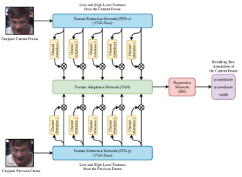
After choosing the GOTURN tracker [20] as our starting point, we extend it using three main extensions. First is the usage of all low and high level features in the tracking process. Making use of the lower level features has already been shown useful in the tracking literature [23, 24]. Second is the usage of a fusion network in the regression network which is adopted from the studies of Akkaya and Halici [25, 26]. Third is the usage of a channel attention mechanism as in the case of He et al. [18]. However, rather than using it for just the static channels of the last two layers, we use it to adaptively weight the dynamically changing channels from all of the layers. Readers who are interested in the detailed step-by-step building procedure of AFTN are referred to the MSc thesis [27] of Alver.

In detail, AFTN is composed of the following four parts:

II-A1 Feature Extraction Network (FEN)

The FENs are composed of convolutional (Conv) layers of the pretrained five-layer VGG-Face [28] network and they act as frozen feature extractors for the previous and current frames. While shallow layers of the FENs extract simple low-level features as edges and corners, the deeper layers extract more complex high-level features as the semantics of the target. Although these high-level features are very useful in tasks that require semantic information, their receptive fields in the input are very large, making them less precise in localizing targets. Therefore, we use both the high-level and low-level features together. Since it is not immediately clear which level features will serve well in tracking, we basically use all them and pass them as inputs to the channel attention networks for adaptive weighting.

II-A2 Channel Attention Network (CAN)

The CANs are simple two-layer multilayer perceptrons (MLP) that are used for weighting the input channels. The first fully connected (FC) layer has 36 units with ReLU activations and the following FC layer has a single unit with a 0.5 biased sigmoid activation corresponding to the weight coefficient for the input channel. These coefficients are then used for weighting the channels according to their importance in tracking. Since we use 5 different layers from the FENs, there are also 5 different CANs. CANs are trained during the offline training process.

II-A3 Feature Adaptation Network (FAN)

The FAN is used for concatenating all the weighted features in their channel dimension. It has no learnable parameters.

II-A4 Regression Network (RN)

The RN is composed of a Conv layer followed by three FC layers and it is used for regressing the target’s bounding box from the input concatenated features. The Conv layer is used as a fusion network for fusing the spatial and semantic information in the concatenated features. It has 256 1$\times$1 kernels with stride 1, zero-padding 0, batch norm with default parameters [29] and ReLU activations. The first two FC layers have 4096 units with ReLU activations and 0.5 dropout [30]. The last FC layer has 3 units with no activations corresponding to the bounding box annotation. As CANs, the RN is also trained during the offline training process.

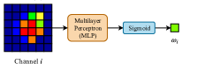
II-B Channel Attention Mechanism

For the task of tracking, some channels in the FENs may be unnecessary or even harmful, whereas some may be very useful. In order to automate this channel selection process, we use a channel attention mechanism with details in Fig. 2. Specifically, we first flatten the 6$\times$6 channels and then pass them through the CANs with biased sigmoid outputs to obtain their weight coefficients. Sigmoids have a bias to ensure that no channel is suppressed down to zero. Since the lower layers in the FENs have channels with sizes 54$\times$54 and 13$\times$13, we first max-pool them to match the 6$\times$6 size of the last layer and then pass them through the CANs. In more detail, for the 54$\times$54 channels, we use two cascaded pooling layers with kernel sizes 6$\times$6 and 3$\times$3 and strides 4 and 2. And for the rest of the 13$\times$13 channels, we use a pooling layer with kernel size 3$\times$3 and stride 2. After the weighting coefficients are obtained, the activations in the channels are multiplied with their corresponding weights. By this way, while the unnecessary features will get suppressed, the useful ones will get pushed up.

Figure 2: The channel attention mechanism that generates the weighting coefficient $\omega_{i}$ for the $i$-th channel.

II-C Dataset

In order to test our proposed face tracker, we use the G1 and G2 sets of the ChokePoint dataset [22]. This dataset contains 30 FPS sequences with frames of size 800$\times$600. However, the annotations provided with it are only the person IDs and eye locations that are not compatible with the task of visual tracking. Thus, we annotate the frames in the G1 and G2 sets with bounding boxes and make the ChokePoint dataset suitable for visual face tracking. This newly formed dataset consists of 432 different video sequences (216 in G1 and 216 in G2) each having only a single person present at a given time and 37,307 frames (16,665 in G1 and 20,652 in G2) with a face. The average length of a sequence is 95.6 frames for G1 and 77.1 frames for G2. For the evaluation, we use the baseline verification protocol for the ChokePoint dataset, where we first use G1 to train our network and use G2 to evaluate it and then do the reverse. In the end, we report the average performances of our trackers on the evaluation sets.

II-D Offline Training and Online Tracking

In the offline training phase, we randomly choose pairs of successive frames from our training dataset with a batch size of 50. We then crop these pair of frames using twice the size of the previous frame’s bounding box and resize them to 224$\times$224 (input size of VGG-Face). We also subtract the mean of the dataset that was used in training VGG-Face. Since we feed the cropped images to the network, we also transform the bounding box annotations of the 800$\times$600 images to the 224$\times$224 ones and use these transformed annotations in the training process. After these preprocessings, we feed the data batch to the network and compute the L1 loss between the ground-truth annotations and the predicted ones. We then backpropagate from this loss and use the Adam optimizer [32] with a constant learning rate of $1e-5$. The training is done for 10 epochs and PyTorch [33] is used for implementation. L2 regularization is applied to the weights with a penalty factor of $1e-3$. Importantly, the network is trained in a fully end-to-end manner.

In the online tracking phase, first, the initial two frames are read from the sequence and the same preprocessing steps in the offline training phase are applied. Then, both of the frames are fed to the network to obtain the bounding box of the current frame within the 224$\times$224 search region. This bounding box is then transformed back to its corresponding location in the 800$\times$600 frame. After this, the current frame is used as the previous frame and a new frame is read as the current frame. Using the predicted bounding box annotation from the previous step, the consecutive frames are again cropped-resized and fed to the network for regressing the bounding box in the newly read frame. This crop-resize-feed-read cycle continues for the rest of the frames and by this way tracking is performed.

II-E Evaluation Metrics

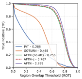
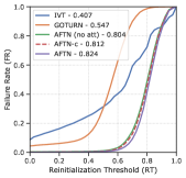
In order to compare the performance of trackers, we use the complementary accuracy and robustness measures that were proposed by C̆ehovin et al. [34, 35]. However, we use slightly different metrics to account for the accuracy and robustness. Specifically, rather than the average overlap, we use the equivalent area under the curve of the True Positive vs. Region Overlap Threshold (TP vs. ROT) plot to account for accuracy. And rather than the failure rate with a single threshold of 0, we use the area above the curve of the Failure Rate vs. Reinitialization Threshold (FR vs. RT) plot to account for robustness. This can be seen as an average of the failure rates for different RTs. These plots have the advantage of displaying the tracker’s performances for not only one, but for thresholds ranging from 0 to 1. In the end, we summarize a tracker’s accuracy and robustness by using the overall score which is just the average of the two. For the speed comparison, we use the FPS values of the trackers.

The TP vs. ROT plot for a sequence is obtained by running a tracker over the sequence and calculating the ratio of frames where the region overlap between the ground-truth and tracker’s bounding box is greater than the ROT. In this plot, the tracker gets reinitialized only if the region overlap becomes 0 (RT is 0). Similarly, the FR vs. RT plot is obtained by again running a tracker over the sequence and calculating the ratio of frames where the region overlap fails below the RT. In this plot, the tracker gets reinitialized if the region overlap falls below the RT.

III Results

The accuracy and robustness values of our proposed tracker (AFTN) are presented in Fig. 3 and Table I. For comparison, we also provide values of the IVT [1] (using the best hyperparameters proposed in the study and forcing it to output squares for fair comparison) and GOTURN [20] (using VGG-Face [28] in place of the AlexNet [36] and again forcing it to output squares for fair comparison) trackers. Among the other surveillance trackers available in the literature, we do not perform comparisons with TLD [2] and DSCT [3] trackers as Dewan et al. [4] have already shown that IVT performs better than the two. Finally, to examine the effect of the attention mechanism and the necessity of using of the previous frame, we also provide values of AFTN (no att) and AFTN-c, which are the versions of AFTN with no attention and no usage of the previous frame, respectively.

Figure 3: The TP vs. ROT (left) and FR vs. RT (right) plots for the IVT, GOTURN, AFTN (no att), AFTN-c and AFTN trackers. The accuracy and robustness values of the trackers are given next to their name in the legend.

TABLE I: Accuracy, robustness, overall scores and speeds of the trackers

Tracker	Accuracy	Robustness	Overall	Speed
IVT	0.288$\pm$0.054	0.407$\pm$0.063	0.348	12.9
GOTURN	0.465$\pm$0.107	0.547$\pm$0.065	0.506	118.6
AFTN (no att)	0.756$\pm$0.075	0.804$\pm$0.038	0.780	148.9
AFTN-c	0.767$\pm$0.079	0.812$\pm$0.036	0.790	183.4
AFTN	0.789$\pm$0.059	0.824$\pm$0.032	0.807	142.9

We see that the proposed AFTN outperforms both IVT and GOTURN by very large margins (overall score of 0.348, 0.506, and 0.807 for IVT, GOTURN, and AFTN, respectively). The IVT tracker performs even worse than the GOTURN tracker. This is expected as traditional trackers like IVT do not make use of the powerful hierarchical features present in deep learning based trackers. We also see that taking away the attention mechanism from AFTN results in a significant drop in the overall score (from 0.807 to 0.780). Lastly, we see that although not using the previous frame as input can cause a drop in the overall score (from 0.807 to 0.790), it can bring a significant jump in the speed (from 142.9 FPS to 183.4 FPS).

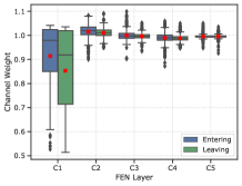
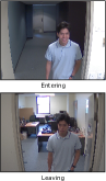
In order to show the effect of the channel attention mechanism, in Fig. 4 we provide detailed information on the average channel weights of AFTN for the entering and leaving scenarios of person with ID 18. First, we see that C1 features get suppressed more compared to the other levels. This is expected as lower level features may contain generic information that is not useful for tracking. We also see that more features from C1 are suppressed in the leaving scenario compared to the entering one (with means of 0.85 and 0.92, respectively). This is also expected as the leaving scenario contains more distracting office objects in the background and the lower level features in C1 contain information on them. It should be noted that the weights for other persons and sequences also show a similar distribution.

Figure 4: The average channel weights (left) of the AFTN in the entering and leaving scenarios of person with ID 18 (right). CX corresponds to the Xth Conv layer in the FENs. Red dots are the means.

In Table I, we also provide the speeds of the trackers with unoptimized codes. It is clear that all of the deep learning based trackers can run at speeds that are very far beyond the 25 FPS requirement for real-time tracking. This is mainly due to the following two aspects: the trackers are trained fully offline with no online updating involved and only a single forward pass is enough for inferring the bounding box annotations. The usage of GPUs, rather than CPUs, is another important aspect that significantly contributes to this. It should be noted that in order to make a fair speed comparison, we ran all trackers on a machine equipped with an Intel Core i7-4790K 8 Core 4.00 GHz CPU and a single NVIDIA GeForce GTX Titan X GPU. We also enabled the benchmark mode of PyTorch during tracking.

From Table I it is clear that the best performing trackers are AFTN and AFTN-c. Among these two, the former one has a higher overall score whereas the latter performs much faster. So which one of these two trackers should be used? If speed is a concern, then AFTN-c can be used as its overall score is comparable to AFTN. However, if the overall score is the major concern, then AFTN should be preferred as it has the highest overall score. So the choice of which tracker to use depends on the objective to maximize.

IV Conclusion

In this letter, we have proposed an attentive deep regression network, an extended version of the GOTURN tracker, for the task of real-time visual face tracking in video surveillance. Experimental results demonstrated that our proposed tracker outperforms the state-of-the-art GOTURN and IVT trackers by very large margins and it achieves speeds ($\sim$140 FPS) that are very far beyond the requirements of real-time tracking. Further, we demonstrated the usefulness of the attention mechanism by showing that not using it can result in a significant drop in the overall score. We also ran experiments to check the necessity of using the previous frame as input and showed that it might not be necessary if speed is the major concern. Additionally, we provided bounding box annotations for the G1 and G2 sets of the ChokePoint dataset and made it suitable for further studies in surveillance face tracking. As a final comment, we highlight the need for more empirical benchmarking studies in (surveillance) face tracking for the rapid advancement of the field.

References

- [1] D. A. Ross, J. Lim, R.-S. Lin, and M.-H. Yang, “Incremental learning for robust visual tracking,” Int. J. Comput. Vision, vol. 77, no. 1-3, pp. 125–141, May 2008. [Online]. Available: http://dx.doi.org/10.1007/s11263-007-0075-7
- [2] Z. Kalal, K. Mikolajczyk, and J. Matas, “Tracking-learning-detection,” IEEE Trans. Pattern Anal. Mach. Intell., vol. 34, no. 7, pp. 1409–1422, Jul. 2012. [Online]. Available: http://dx.doi.org/10.1109/TPAMI.2011.239
- [3] Q. Wang, Feng Chen, Wenli Xu, and M. Yang, “Online discriminative object tracking with local sparse representation,” in 2012 IEEE Workshop on the Applications of Computer Vision (WACV), Jan 2012, pp. 425–432.
- [4] M. A. A. Dewan, E. Granger, F. Roli, R. Sabourin, and G. L. Marcialis, “A comparison of adaptive appearance methods for tracking faces in video surveillance,” in 5th International Conference on Imaging for Crime Detection and Prevention (ICDP 2013), Dec 2013, pp. 1–7.
- [5] X. Lan, Z. Xiong, W. Zhang, S. Li, H. Chang, and W. Zeng, “A super-fast online face tracking system for video surveillance,” in 2016 IEEE International Symposium on Circuits and Systems (ISCAS), May 2016, pp. 1998–2001.
- [6] Y. LeCun, Y. Bengio, and G. Hinton, “Deep learning,” nature, vol. 521, no. 7553, p. 436, 2015.
- [7] J. Schmidhuber, “Deep learning in neural networks: An overview,” Neural Networks, vol. 61, pp. 85–117, 2015, published online 2014; based on TR arXiv:1404.7828 [cs.NE].
- [8] A. Krizhevsky, I. Sutskever, and G. E. Hinton, “Imagenet classification with deep convolutional neural networks,” in Advances in Neural Information Processing Systems, p. 2012.
- [9] K. Simonyan and A. Zisserman, “Very deep convolutional networks for large-scale image recognition,” CoRR, vol. abs/1409.1556, 2014.
- [10] R. B. Girshick, J. Donahue, T. Darrell, and J. Malik, “Rich feature hierarchies for accurate object detection and semantic segmentation,” 2014 IEEE Conference on Computer Vision and Pattern Recognition, pp. 580–587, 2014.
- [11] S. Hong, H. Noh, and B. Han, “Decoupled deep neural network for semi-supervised semantic segmentation,” in NIPS, 2015.
- [12] E. Shelhamer, J. Long, and T. Darrell, “Fully convolutional networks for semantic segmentation,” IEEE Trans. Pattern Anal. Mach. Intell., vol. 39, no. 4, pp. 640–651, Apr. 2017. [Online]. Available: https://doi.org/10.1109/TPAMI.2016.2572683
- [13] Y. Taigman, M. Yang, and L. Wolf, “L.: Deepface: Closing the gap to human-level performance in face verification,” in In: IEEE CVPR, 2014.
- [14] M. Kristan, J. Matas, A. Leonardis, M. Felsberg, L. Čehovin Zajc, G. Fernandez, and et al., “The visual object tracking vot2015 challenge results,” in Visual Object Tracking Workshop 2015 at ICCV2015, Dec 2015.
- [15] M. Kristan, A. Leonardis, J. Matas, M. Felsberg, R. Pflugfelder, L. Čehovin Zajc, T. Vojir, G. Häger, A. Lukežič, G. Fernandez, and et al., “The visual object tracking vot2016 challenge results,” Springer, Oct 2016. [Online]. Available: http://www.springer.com/gp/book/9783319488806
- [16] M. Kristan, A. Leonardis, J. Matas, M. Felsberg, R. Pflugfelder, L. Čehovin Zajc, T. Vojir, G. Häger, A. Lukežič, A. Eldesokey, G. Fernandez, and et al., “The visual object tracking vot2017 challenge results,” 2017. [Online]. Available: http://openaccess.thecvf.com/content_ICCV_2017_workshops/papers/w28/Kristan_The_Visual_Object_ICCV_2017_paper.pdf
- [17] M. Kristan, A. Leonardis, J. Matas, M. Felsberg, R. Pfugfelder, L. C. Zajc, T. Vojir, G. Bhat, A. Lukezic, A. Eldesokey, G. Fernandez, and et al., “The sixth visual object tracking vot2018 challenge results,” 2018.
- [18] A. He, C. Luo, X. Tian, and W. Zeng, “A twofold siamese network for real-time object tracking,” 2018 IEEE/CVF Conference on Computer Vision and Pattern Recognition, pp. 4834–4843, 2018.
- [19] Q. Wang, Z. Teng, J. Xing, J. Gao, W. Hu, and S. Maybank, “Learning attentions: Residual attentional siamese network for high performance online visual tracking,” in The IEEE Conference on Computer Vision and Pattern Recognition (CVPR), June 2018.
- [20] D. Held, S. Thrun, and S. Savarese, “Learning to track at 100 fps with deep regression networks,” in European Conference Computer Vision (ECCV), 2016.
- [21] S. Krebs, B. Duraisamy, and F. Flohr, “A survey on leveraging deep neural networks for object tracking,” 2017 IEEE 20th International Conference on Intelligent Transportation Systems (ITSC), pp. 411–418, 2017.
- [22] Y. Wong, S. Chen, S. Mau, C. Sanderson, and B. C. Lovell, “Patch-based probabilistic image quality assessment for face selection and improved video-based face recognition,” in IEEE Biometrics Workshop, Computer Vision and Pattern Recognition (CVPR) Workshops. IEEE, June 2011, pp. 81–88.
- [23] C. Ma, J.-B. Huang, X. Yang, and M.-H. Yang, “Hierarchical convolutional features for visual tracking,” in Proceedings of the 2015 IEEE International Conference on Computer Vision (ICCV), ser. ICCV ’15. Washington, DC, USA: IEEE Computer Society, 2015, pp. 3074–3082. [Online]. Available: http://dx.doi.org/10.1109/ICCV.2015.352
- [24] L. Wang, W. Ouyang, X. Wang, and H. Lu, “Visual tracking with fully convolutional networks,” 2015 IEEE International Conference on Computer Vision (ICCV), pp. 3119–3127, 2015.
- [25] I. B. Akkaya, “Mouse Face Tracking Using Convolutional Neural Networks,” M.Sc. Thesis, Department of Electrical and Electronics Engineering, Middle East Technical University, Ankara, Turkey, 2016.
- [26] I. B. Akkaya and U. Halici, “Mouse face tracking using convolutional neural networks,” IET Computer Vision, vol. 12, no. 2, pp. 153–161, 2018.
- [27] S. Alver, “Attentive Deep Regression Networks for Real-Time Visual Face Tracking in Video Surveillance,” M.Sc. Thesis, Department of Electrical and Electronics Engineering, Middle East Technical University, Ankara, Turkey, 2019.
- [28] O. M. Parkhi, A. Vedaldi, and A. Zisserman, “Deep face recognition,” in British Machine Vision Conference, 2015.
- [29] S. Ioffe and C. Szegedy, “Batch normalization: Accelerating deep network training by reducing internal covariate shift,” CoRR, vol. abs/1502.03167, 2015. [Online]. Available: http://arxiv.org/abs/1502.03167
- [30] N. Srivastava, G. Hinton, A. Krizhevsky, I. Sutskever, and R. Salakhutdinov, “Dropout: A simple way to prevent neural networks from overfitting,” Journal of Machine Learning Research, vol. 15, pp. 1929–1958, 2014. [Online]. Available: http://jmlr.org/papers/v15/srivastava14a.html
- [31] D. E. King, “Dlib-ml: A machine learning toolkit,” Journal of Machine Learning Research, vol. 10, pp. 1755–1758, 2009.
- [32] D. P. Kingma and J. Ba, “Adam: A method for stochastic optimization,” CoRR, vol. abs/1412.6980, 2014. [Online]. Available: http://arxiv.org/abs/1412.6980
- [33] A. Paszke, S. Gross, S. Chintala, G. Chanan, E. Yang, Z. DeVito, Z. Lin, A. Desmaison, L. Antiga, and A. Lerer, “Automatic differentiation in pytorch,” in NIPS-W, 2017.
- [34] L. Čehovin Zajc, M. Kristan, and A. Leonardis, “Is my new tracker really better than yours?” in WACV 2014: IEEE Winter Conference on Applications of Computer Vision. IEEE, Mar 2014. [Online]. Available: http://prints.vicos.si/publications/302
- [35] L. Cehovin, A. Leonardis, and M. Kristan, “Visual object tracking performance measures revisited,” IEEE Transactions on Image Processing, vol. 25, pp. 1261–1274, 2016.
- [36] A. Krizhevsky, I. Sutskever, and G. E. Hinton, “Imagenet classification with deep convolutional neural networks,” in Advances in Neural Information Processing Systems (NIPS 2012), 2012, p. 4.