Almost-rigidity of frameworks

Abstract

We extend the mathematical theory of rigidity of frameworks (graphs embedded in $d$-dimensional space) to consider nonlocal rigidity and flexibility properties. We provide conditions on a framework under which (I) as the framework flexes continuously it must remain inside a small ball, a property we call “almost-rigidity”; (II) any other framework with the same edge lengths must lie outside a much larger ball; (III) if the framework deforms by some given amount, its edge lengths change by a minimum amount; (IV) there is a nearby framework that is prestress stable, and thus rigid. The conditions can be tested efficiently using semidefinite programming. The test is a slight extension of the test for prestress stability of a framework, and gives analytic expressions for the radii of the balls and the edge length changes. Examples illustrate how the theory may be applied in practice, and we provide an algorithm to test for rigidity or almost-rigidity. We briefly discuss how the theory may be applied to tensegrities.

1 Introduction

Frameworks are graphs with fixed edge lengths embedded in a Euclidean space. Studied for their mathematical properties for decades, they also arise as models in a great many applications: from engineering macroscale structures, such as sculptures [tensegritree], play structures [Pietroni:2017epa], or the Kurilpa bridge in Brisbane [kurilpa]; to designing the microstructure of materials with novel properties [Paulose:2015hd, RayneauKirkhope:2017cy, Borcea:2017jf, bertholdi], to studying arrangements of jammed particles [Liu:2010jx, sticky, henkes], to understanding allostery in biology [Yan:2017cu, Rocks:2017bu]; to studying the properties of molecules [Whiteley:2005hj, Sartbaeva:2006ks, HolmesCerfon:2017hz]; to analyzing the structure of proteins [Jacobs:2001we]; to studying origami folding [Demaine:2007jh]. A question of interest in all of these areas is whether a framework is locally rigid, meaning the only continuous motions of the vertices that preserve the lengths of the edges are rigid-body motions. Mathematical rigidity theory provides various sufficient conditions under which a framework is guaranteed to be locally rigid. For so-called generic embeddings of the graph (roughly, random edge lengths), it is often sufficient to test a combinatorial property of the graph itself, but for specific embeddings the outcome of the tests depends on the particular edge lengths of interest.

A challenge that arises when applying these tests to the problems above, is that often one does not only wish to understand rigidity properties for a given, fixed set of edge lengths; one may wish to understand nearby configurations, or to allow the edge lengths to change. For example, in molecular dynamics, bonds between particles are never fixed at exactly one length, but rather they vibrate around that length, and this can change the geometry or topology of their configuration space. In engineering applications, one may design a framework on a computer to be rigid, but when one builds it the edges are always slightly different from the designed ones, so it may not be as rigid. Even when testing for rigidity on a computer, calculations can only be performed to finite precision, and even small rounding errors can change the outcome of a rigidity test.

Fortunately, the strongest sufficient condition for local rigidity, infinitesimal rigidity, is robust to small perturbations. However, a weaker but still important condition, called prestress stability, is not robust to any size of perturbation. Prestress stability has nothing to say about the rigidity or flexibility of nearby configurations, nor about how these might change if the edges can change lengths. In fact, as we show later, a prestress stable framework that is perturbed by even the smallest amount can become flexible.

Our main contribution is to introduce a theory aimed at understanding the rigidity properties of frameworks that are close to a framework of interest, and at controlling the edge changes for frameworks that undergo small deformations. We call this theory almost rigidity, because it allows us to talk about frameworks that are not perfectly rigid, but nevertheless cannot flex very far in configuration space. The theory extends the theory of prestress stability to extract quantitative information about nonlinear deformations of a framework near a rigid configuration.

Our contribution is laid out in four main theorems, labelled (I)–(IV), which are introduced informally here and stated more precisely in Section 3. The theorems are illustrated schematically in Figure 1. The theorems concern a framework, which is a pair $(p,\mathcal{E})$ such that $p=(p_{1},p_{2},\ldots,p_{n})^{T}\in\mathbb{R}^{dn}$ is the configuration of the framework, representing the positions of $n$ vertices in $d$-dimensional space, and $\mathcal{E}=\{(i_{1},j_{1}),\ldots,(i_{m},j_{m})\}$ lists the $m$ edges of a graph connecting the vertices. We show that when certain sufficient conditions are established for the framework, conditions that are similar to but less restrictive than the conditions for prestress stability [Connelly:1996vja], then:

1. There is a ball of radius $\eta_{1}$, such that if $p$ flexes continuously with fixed edge lengths to some other configuration $p^{\prime}$, then $|p^{\prime}-p|\leq\eta_{1}$, where $|\cdot|$ is the $l_{2}$-norm.

We call a framework satisfying the conditions of (I) almost-rigid, because it implies that even though the framework is flexible, it can’t flex very much (since $\eta_{1}$ is usually much smaller than a typical edge length.) So (I) is a form of rigidity in that it constrains a configuration to stay in a small region of configuration space.

1. There is a ball of radius $\eta_{2}>\eta_{1}$ such that if configuration $q$ has the same edge lengths as $p$, and $|q-p|>\eta_{1}$, then $|q-p|\geq\eta_{2}$.

This theorem is an extension of the concept of global rigidity, which concerns frameworks with exactly one embedding. When this theorem holds, there may be other embeddings of the framework (i.e. different from $p$), but if they are not sufficiently close to $p$, then they must lie sufficiently far away.

1. If $p$ is deformed continuously to some configuration $q$ with the same edge lengths as $p$ and such that $|q-p|>\eta_{2}$, there must be some point $q^{\prime}$ on the deformation path such that the vector of squared edge lengths, $e(q^{\prime})$, satisfies $|e(q^{\prime})-e(p)|\geq e_{\rm min}^{*}$.

This theorem gives a lower bound for how much we must stretch the edges of a framework to deform it into another, sufficiently distant, embedding with the same edge lengths.

1. There is a nearby framework $q$ with $|q-p|\leq\eta_{1}$, such that $q$ is rigid.

This last theorem may be used as a numerical test for rigidity, if we are in the unfortunate case when the framework of interest is rigid, but when represented on a computer it is flexible. We give examples of such frameworks in Section 2.2.

We give analytic expressions for $\eta_{1}$,$\eta_{2}$, and $e_{\rm min}^{*}$, that can be evaluated with linear algebra and semidefinite programming. The results in this paper can be applied without either testing exactly for zero, or determining in advance a cutoff value below which numerical quantities are treated as zero. Any observed measurement of a real configuration or numerical approximation to coordinates can be used to obtain a meaningful conclusion.

We prove Theorems (I)–(IV) by constructing an energy function, $H(q)$, that depends only on the edge lengths of a configuration $q$. We derive conditions under which $H(q)>H(p)$ for $q$ in an annulus, $|q-p|\in(\eta_{1},\eta_{2})$. This is sufficient to prove Theorems (I),(II). To prove Theorem (III) we calculate a lower bound for $H(q)-H(p)$ along any path across the annulus. For Theorem (IV), which depends on stronger conditions than the other theorems, we show that $H(q)$ has an isolated local minimum at $p_{\rm pss}$ sufficiently close to $p$, which is sufficient for $p_{\rm pss}$ to be locally rigid. The function $H(q)$ has a physical interpretation as an energy, since it is constructed by pretending the edges of the framework are springs and some of the springs are under tension or compression.

The rest of the paper proceeds as follows. First, we review various tests for local rigidity in Section 2, and give examples to show their limitations. We set up and state our main theorems in Section 3, and illustrate them on several examples in Section 4. The rest of the paper will be devoted to proving these theorems. To do this we develop some results concerning the shape of a general three-times continuously differentiable function near a point that is nearly a critical point, in Section 5. These results, which extend the second derivative test, may be of independent interest. In Section LABEL:sec:energyfunction we construct a particular energy function $H(q)$ associated with a framework $(p,\mathcal{E})$ and discuss its properties. Finally in Section LABEL:sec:theoremproofs we prove our main theorems by applying our general propositions from Section 5 to $H(q)$. We briefly explain how to extend these results to tensegrities in Section LABEL:sec:tens, and we conclude in Section LABEL:sec:conclusion.

Figure 1: Schematic of our Theorems presented in Section 3, concerning the configuration space $\mathcal{C}^{p}\subset\mathbb{R}^{dn}$ near a given framework $p\in\mathbb{R}^{dn}$. Framework $p$ may be flexible (solid black path), but Theorem I says that if it flexes continuously with fixed edge lengths, it stays within a ball of radius $\eta_{1}$. There may be other configurations with the same edge lengths as $p$ (dashed black line), but Theorem II says that if they are not in the ${\color[rgb]{0.7,0.11,0.11}\eta_{1}}$-ball, then they lie outside a ball of radius $\eta_{2}$ $>{\color[rgb]{0.7,0.11,0.11}\eta_{1}}$. To deform continuously from $p$ to some configuration $q$ outside the ball of radius $\eta_{2}$, Theorem III says that the $l_{2}$-norm of the list of squared edge lengths must change by at least an amount $e_{\rm min}^{*}$. Finally, Theorem IV says there is a configuration $p_{\rm pss}$ within the ball of radius $\eta_{1}$ that is prestress stable (and rigid). All of these results depend on verifying conditions on $p$, which generalize the test for prestress stability, and the results of this test gives analytic formulas for ${\color[rgb]{0.7,0.11,0.11}\eta_{1}}$, $\eta_{2}$, $e_{\rm min}^{*}$.

2 Review of mathematical rigidity theory

2.1 First-order rigidity, second-order rigidity, and prestress stability

Figure 2: Schematic illustrating different kinds of local rigidity and how they are related. Examples show frameworks with different kinds of rigidity. (A) First-order rigid in $\mathbb{R}^{2}$ (but flexible in $\mathbb{R}^{3}$.) (B) Prestress stable in $\mathbb{R}^{2}$. (C) Same as B, with two infinitesimal flexes plotted as arrows (green, yellow) and colors on the bars are proportional to values of the self-stress. Bright blue is the most positive (like a cable, that wants to shrink), and bright red the most negative (like a strut, that wants to expand.) (D) Same as B, but vertices 5, 6 have been perturbed vertically. This framework is flexible in $\mathbb{R}^{2}$, because vertices 5 and 6 can move up and down, but they can’t move by very much.

In this section we review the mathematical theory of local rigidity. We start from the definition that a framework $(p,\mathcal{E})$ with edge lengths $d_{ij}$ is locally rigid if it is an isolated solution (modulo translations and rotations) to the following system of algebraic equations:

$$f_{ij}(p):=|p_{i}-p_{j}|^{2}-d_{ij}^{2}=0\,\qquad(i,j)\in\mathcal{E}\,.$$ (2.1)

Testing for local rigidity is co-NP-hard in general [Demaine:2007jh, Abbott:2008tj]. This leads to the study of sufficient conditions for rigidity that are easier to test.

To motivate these conditions it is helpful to consider a continuous, analytic deformation $p(t)$ with $p(0)=p$ (we are abusing notation here), and trying to solve (2.1) locally. Taking $\frac{d}{dt}$ of (2.1) and evaluating at $t=0$ gives

$$(p_{i}-p_{j})\cdot(v_{i}-v_{j})=0\,\qquad(i,j)\in\mathcal{E}\,,$$ (2.2)

where $v=p^{\prime}(0)$ and $v_{i}\in\mathbb{R}^{d}$ are the components of $v$ corresponding to the $i$th vertex. A vector $v$ which solves (2.2) is called an infinitesimal flex. Physically, a vector $v\in\mathbb{R}^{dn}$ corresponds to a set of velocities for the vertices. It is an infinitesimal flex if, when the framework is deformed as $x\to x+\delta v$ for some small $\delta$, the edge lengths do not change at $O(\delta)$. An infinitesimal flex corresponding to an infinitesimal rigid-body motion is called a trivial flex; we write the subspace of trivial flexes $\mathcal{T}=\mathcal{T}(p)$. This space depends on the particular configuration, but we sometimes omit this dependence in the notation.

Another way to write (2.2) is

$$R(p)v=0\,,$$ (2.3)

where $R(p)\in\mathbb{R}^{m\times dn}$ is the rigidity matrix. If the $k$th edge is $(i_{k},j_{k})$, then the $k$th row of the rigidity matrix is constructed as $R_{k,(d-1)i_{k}+1:di_{k}}=p_{i_{k}}-p_{j_{k}}$, $R_{k,(d-1)j_{k}+1:dj_{k}}=-(p_{i_{k}}-p_{j_{k}})$, with zeros everywhere else.

If there are no solutions $v$ to (2.3) except trivial flexes, then we say that $(p,\mathcal{E})$ is first-order rigid (also called infinitesimally rigid.) An example of a framework that is first-order rigid is given in Figure 2 (A). A theorem from rigidity theory says that if $(p,\mathcal{E})$ is first-order rigid, then it is rigid [e.g. Asimow:1978ena]. Clearly, testing for first-order rigidity is efficient whenever computing the null space of a matrix is efficient.

A technical but important point is that in practice, to remove trivial flexes from consideration, one typically defines a subspace $\mathcal{C}$ to be a subspace complementary to $\mathcal{T}$, i.e. such that $\mbox{Span}\{\mathcal{C},\mathcal{T}\}=\mathbb{R}^{dn}$ and $\mathcal{C}\cap\mathcal{T}=\{0\}$. Some possibilities include setting $\mathcal{C}=\mathcal{T}^{\perp}$, or pinning (freezing the values of) $d(d+1)/2$ vertex coordinates [whitewhiteley, anchored], or letting $\mathcal{C}$ be a random $dn-d(d+1)/2$-dimensional subspace. Then a framework is first-order rigid if $\mbox{Null}(R(p))\cap\mathcal{C}$ is empty.

If $(p,\mathcal{E})$ is not first-order rigid, then it could be either rigid or flexible. To go further, take $\frac{d^{2}}{dt^{2}}$ of (2.1) and evaluate at $t=0$:

$$(p_{i}-p_{j})\cdot(a_{i}-a_{j})+(v_{i}-v_{j})\cdot(v_{i}-v_{j})=0\,\qquad(i,j)\in\mathcal{E}\,.$$ (2.4)

Here $a=p^{\prime\prime}(0)$ has the physical interpretation of the acceleration of the vertices. Another way to write (2.4) is

$$R(p)a=-R(v)v\,.$$ (2.5)

If there are no solutions $(v,a)$ with non-trivial flexes $v$ to the system (2.3),(2.5), then the framework $(p,\mathcal{E})$ is second-order rigid. A theorem from rigidity theory says that if $(p,\mathcal{E})$ is second-order rigid, then it is rigid [Connelly:1980joa]. Neither this theorem, nor the one for first-order rigidity, are trivial statements, because it could be that $p$ lies at a “cusp” in configuration space, so that there is a continuous deformation $p(t)$ but its first $k$ derivatives are zero, i.e. $p^{\prime}(0)=p^{\prime\prime}(0)=\cdots=p^{(k)}(0)=0$, $p^{(k+1)}\neq 0$ [Connelly:1994fz].

Testing for second-order rigidity seems to be difficult. To show second-order rigidity, one has to show that for each $v\in\mbox{Null}(R(p))\cap\mathcal{C}$, there is no solution $a$ to (2.5). If we fix $v$, then (2.5) becomes a linear system in $a$. Since the column span of $R(p)$ is orthogonal to $\mbox{Null}(R^{T}(p))$, either there is a solution or

$$\exists\omega\in\mbox{Null}(R^{T}(p)):\quad\;\omega^{T}R(v)v>0\,,$$ (2.6)

which witnesses that $R(v)v$ is not in the column span of $R(p)$. (This is the Fredholm alternative.)

In principle, one could show that there is no solution to (2.5) for any $v\in\mbox{Null}(R(p))\cap\mathcal{C}$, by finding an $\omega$ solving (2.6) for each such $v$, but without fixing $v$, this is a nonlinear problem with no known efficient algorithm to solve it.

Therefore one usually considers a version of rigidity that is stronger than second-order rigidity, but still weaker than first-order rigidity. Suppose that

$$\exists\omega\in\mbox{Null}(R^{T}(p)):\qquad\omega^{T}R(v)v>0\qquad\forall v\in\mbox{Null}(R(p))\cap\mathcal{C}\,.$$ (2.7)

That is, a single $\omega$ works for all $v$ in (2.6), so clearly (2.6) holds for each $v$. So, $(p,\mathcal{E})$ is second-order rigid, and hence rigid. A framework satisfying (2.7) is said to be prestress stable. An example of a framework that is prestress stable is given in Figure 2 (B). This figure also shows how the various flavours of local rigidity are nested within each other.

An important element in (2.7) is the vector $\omega$. Any vector $\omega\in\mathbb{R}^{m}$ is called a stress, and if in addition $\omega\in\mbox{Null}(R^{T}(p))$ it is called a self-stress (also called an equilibrium stress.) Physically, a stress is an assignment of tensions to the edges, so the edges behave like springs which are under tension or compression. It is a self-stress if the forces on the edges are balanced at each node, so the framework is local force equilibrium with that assignment of tensions. To see the connection between forces and the left null space of the rigidity matrix, write $(\omega^{T}R(p))_{i}=\sum_{j:(i,j)\in\mathcal{E}}\omega_{ij}(p_{i}-p_{j})$, where $\omega_{ij}$ is the component of $\omega$ associated with edge $(i,j)$. Since $\omega_{ij}(p_{i}-p_{j})$ is the force applied at vertex $i$ by the edge $(i,j)$, if $\omega$ is a self-stress, the sum of the forces at each vertex is zero.

One major advantage of prestress stability is that it is possible to test this property using semidefinite programming, which is efficient for many problems. To see how, observe that the term $\omega^{T}R(v)v$ is quadratic in velocities and linear in stresses. Therefore, we can write this term as $v^{T}\Omega(\omega)v$, where $\Omega(\omega)\in\mathbb{R}^{dn\times dn}$ is the stress matrix associated with a stress $\omega$, defined so that it acts on flexes as $u^{T}\Omega v=\sum_{(i,j)\in\mathcal{E}}\omega_{ij}(u_{i}-u_{j})\cdot(v_{i}-v_{j})$. Clearly the stress matrix is symmetric. Then, (2.7) can be written as

$$\exists\omega\in\mathcal{W}^{0}:\quad\;v^{T}\Omega(\omega)v>0\qquad\forall v\in\mathcal{V}^{0}\,,$$ (2.8)

where we defined the linear spaces of nontrivial infinitesimal flexes, and self-stresses respectively, as

$$\mathcal{V}^{0}=\mbox{Null}(R(p))\cap\mathcal{C}\,,\qquad\mathcal{W}^{0}=\mbox{Null}(R^{T}(p))\,.$$ (2.9)

That is, we must find a matrix $\Omega$ within a linear space of symmetric matrices, that is positive definite on a linear subspace. This is a convex problem, so may be solved using algorithms that have polynomial complexity and are often efficient in practice.

Here is one algorithm to solve it. Let $n_{v}=\mbox{dim}(\mathcal{V}^{0})$, $n_{w}=\mbox{dim}(\mathcal{W}^{0})$; we assume $n_{v},n_{w}\geq 1$. Let $I_{n_{v}}\in\mathbb{R}^{n_{v}\times n_{v}}$ be the identity matrix. Let $V$ be a matrix whose columns form an orthonormal basis of $\mathcal{V}^{0}$, and let $\{w_{i}\}_{i=1}^{n_{w}}$ be an orthonormal basis of $\mathcal{W}^{0}$. Let $M_{i}=V^{T}\Omega(w_{i})V$. Solve the following problem for unknown variables $t\in\mathbb{R}$, $a\in\mathbb{R}^{n_{w}}$, $X\in\mathbb{R}^{n_{v}\times n_{v}}$:

$$\underset{t,a,X}{\text{maximize}} t$$ (2.10)

subject to $$X=\sum_{i=1}^{n_{w}}a_{i}M_{i}-tI_{n_{v}},$$

$$X\succeq 0,$$

$$\left(\sum_{i=1}^{n_{w}}a_{i}^{2}\right)^{1/2}\leq 1.$$

The notation $A\succeq\lambda$ ($A\succ\lambda$) for a symmetric matrix $A$ means that $A-\lambda I$ is positive semidefinite (positive definite), where $I$ is the identity matrix with the same dimensions as $A$. Equivalently, $\lambda_{\rm min}(A)\geq\lambda$, where $\lambda_{\rm min}(A)$ is the smallest eigenvalue of a matrix $A$.

The above optimization program can be input nearly verbatim into standard convex optimization software; we use CVX for the examples in this paper [cvx, gb08]. The optimal stress and eigenvalue are extracted from the optimal solution $(t_{\rm opt},a_{\rm opt},X_{\rm opt})$ as

$$\omega=\sum_{i=1}^{n_{w}}(a_{\rm opt})_{i}w_{i}\,,\qquad\lambda_{0}=t_{\rm opt}\,.$$

The test is successful if $t_{\rm opt}>0$.

There are two special cases for which the convex optimization program (2.10) need not be run:

• If $n_{w}=1$, so there is only one self- stress $w_{1}$, then we merely check the eigenvalues of $M_{1}$. If they are all of the same sign, say with absolute values $0<\lambda_{1}\leq\lambda_{2}\leq\cdots$, then we set $\lambda_{0}=\lambda_{1}$, and $\omega=\mbox{sgn}(\lambda_{1})w_{1}$. If the eigenvalues are not all of the same sign, or if some are zero, the test is unsuccessful.

• If $n_{v}=1$, so there is only one infinitesimal flex, then each $M_{i}$ is a scalar. If one of the $M_{i}$ is nonezro, set $\lambda_{0}=\max_{i}|M_{i}|$, and set $\omega=\mbox{sgn}(M_{i})w_{i}$, where $i=\operatorname*{arg\,max}_{i}|M_{i}|$. If all the $M_{i}$ are zero, the test is unsuccessful.

2.2 A challenge in testing for prestress stability

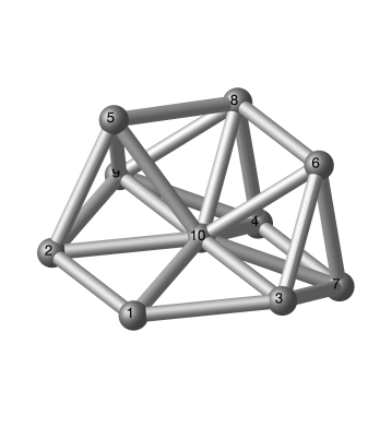
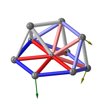
Figure 3: Left: A packing of $N=10$ unit spheres that has $3N-7=23$ contacts, fewer than the $3N-6$ needed generically to be rigid. Nevertheless, this packing is rigid. Middle: a representation of the packing as a framework, with vertices at the sphere centers and edges between spheres in contact. Right: the self-stress, as colors on bars, (blue is positive, like a cable that wants to shrink, and red is negative, like a strut that wants to expand), and the two infinitesimal flexes (yellow and green arrows.) The infinitesimal flexes are calculated assuming spheres 2,10,3 are pinned.

In this section we introduce two examples to illustrate a challenge that can occur in testing for rigidity when a prestress stable framework is perturbed.

2.2.1 Example 1

Consider framework (B) in Figure 2. This framework has 6 vertices, 9 edges, and 3 rigid-body degrees of freedom. When the vertices are placed generically (e.g. randomly), it has $6\times 2-3-8=1$ nontrivial degree of freedom, making it flexible. However, for the particular embedding in the figure, where vertices $1,5,6,2$ are colinear, the framework acquires one self-stress and a second non-trivial infinitesimal-flex (Figure 2(C)), and the corresponding stress matrix is positive definite on the flex space as in (2.7). Therefore, this framework is prestress stable, and hence rigid.

If we perturb this framework, however, it is no longer rigid. For example, in Figure 2(D), vertices 5,6 have been perturbed vertically by 5% of the length of edge 1-2, so they are no longer colinear with vertices 1,2. We calculated the left and right null spaces of the rigidity matrix $R(p)$ on a computer, and found the framework has a one-dimensional space of nontrivial flexes, and a zero-dimensional space of self-stresses. Therefore it cannot be prestress stable; indeed it flexible. This is true no matter how little vertices 5,6 are perturbed vertically; even a perturbation as small as $10^{-14}$ destroys the extra flex and stress (results from [whitewhiteley] give a formal proof.)

Notably, in this example, it is also clear that if vertices 1,2 are pinned (to remove the trivial Euclidean motions), then vertices 5,6 can move, but not very far. As the framework deforms, it remains “close to” the prestress stable configuration B, even though it never adopts this configuration. Yet, the rigidity test above is blind to the fact that the framework is constrained to move in a small region, nor can it detect there is a nearby prestress stable configuration.

This example is somewhat contrived, so we turn to a more physically motivated example with the same basic properties.

2.2.2 Example 2

Consider the cluster formed from $N=10$ unit spheres in 3 dimensions shown in Figure 3. Clusters such as these are of interest in materials science, since the arrangements of small groups of particles can explain certain macroscopic properties of materials, such as how they form gels and glassy phases [PatrickRoyall:2008fz, Manoharan:2015ko, Robinson:2019et]. This particular sphere cluster was discovered in [HolmesCerfon:2016wa], which presented a nearly complete dataset of rigid packings of $N\leq 14$ unit spheres.

The sphere cluster can be represented as a framework by putting a vertex at the center of each sphere, and an edge between spheres in contact. The induced framework has 10 vertices, so requires 30 variables to describe the positions of the vertices. It has 23 edges, and when the vertices are placed generically, this framework has 30-23=7 degrees of freedom. Of these, 6 correspond to rigid-body motions (three rotations and three translations), so generically this framework is flexible, with 1 nontrivial degree of freedom. Nevertheless, when this framework is formed from edges that are all unit length, it can be argued to be rigid (see [HolmesCerfon:2016wa].)

The numerical configuration of the framework that is plotted was found on a computer by solving (2.1) numerically with $d_{ij}=1$. Because computers have finite precision, the solver did not find the exact solution $p_{\rm true}$. Rather, it found an approximate solution $p$ such that

$$|f_{ij}(p)|=\big{|}|p_{i}-p_{j}|^{2}-d_{ij}^{2}\big{|}\leq\delta\,,\qquad(i,j)\in\mathcal{E}\,,$$ (2.11)

where $\delta>0$ is a numerical tolerance parameter, chosen to be $\delta=4\varepsilon\approx 9\times 10^{-16}$ where $\varepsilon\approx 2.2204\times 10^{-16}$ is machine precision. The numerical solution $p$ is a perturbation of $p_{\rm true}$, so it should behave like a generic embedding, and should be flexible. Indeed, we calculated the rigidity matrix $R(p)$ and found it has a one-dimensional right null space, and a zero-dimensional left null space, so $p$ cannot be prestress stable.

However, if we look at the singular values of $R(p)$, they tell a more nuanced story. The singular values in increasing order are

$$6.6\times 10^{-9},\;0.47,\;0.54,\;0.76,\;0.82,\;0.90,\;1.01,\;1.15,\;1.18,\;1.19,\;1.28,\;1.30,\;1.35,\;$$

$$1.45,\;1.48,\;1.59,\;1.66,\;1.72,\;1.77,\;1.86,\;1.90,\;2.22,\;2.33\,.$$

The smallest singular value, $\sigma_{0}=6.6\times 10^{-9}$, is many orders of magnitude smaller than the second-smallest, $0.47$. The right and left singular vectors corresponding to $\sigma_{0}$, call them $v$ and $w$ respectively, are “almost” a true flex and stress. That is, if we flex the framework in direction $v$, the edge lengths change at a rate proportional to $\sigma_{0}$, hence very little. Similarly, if we put the edges under tension according to stress $w$, the imbalance of forces at each node is proportional to $\sigma_{0}$, hence very small. Can the almost-flex and almost-stress be used to gain more information about how framework $p$ can actually flex?

A natural idea is to include the almost-flex $v$ and almost-stress $w$ in the test (2.8) for prestress stability. To this end we formed the “almost flex space” $\mathcal{V}=(\mbox{Null}(R(p))\oplus v)\ \cap\mathcal{C}$, and the “almost self-stress space” $\mathcal{W}=\mbox{Null}(R^{T}(p))\oplus w$. Then $\mbox{dim}(\mathcal{V})=2$, $\mbox{dim}(\mathcal{W})=1$. We performed test (2.8) using $\mathcal{V},\mathcal{W}$ in the place of $\mathcal{V}^{0},\mathcal{W}^{0}$, by forming the “almost” self-stress matrix $\Omega=\Omega(w)$ (setting $|w|=1$), and computing the eigenvalues of $V^{T}\Omega V$, where $V$ is an orthonormal basis of $\mathcal{V}$. We obtained

$$\mbox{eig}(V^{T}\Omega V)=\{0.33,0.46\}\,.$$

The almost-self-stress matrix $\Omega$ is positive definite on the almost-flex space $\mathcal{V}$.

Unfortunately, this test doesn’t show that $p$ is rigid, since $\mathcal{V}$, $\mathcal{W}$ are not true flexes and self-stresses. What then does it show?

One approach to answering this question (an approach we will not follow in this paper) would be to assume that $|p-p_{\rm true}|$ is sufficiently small, and in addition, that any sufficiently small singular values of $R(p)$ are perturbations of zero singular values of $R(p_{\rm true})$. Then, $v$ and $w$ are simply perturbations of a true flex $v_{\rm true}$ and a true stress $w_{\rm true}$ of $p_{\rm true}$. One can then use perturbation bounds from linear algebra to show that $|v-v_{\rm true}|$, $|w-w_{\rm true}|$ are both small, so the eigenvalues of $V^{T}\Omega V$ are close to those of $V^{T}_{\rm true}\Omega_{\rm true}V_{\rm true}$. Therefore, if $V^{T}\Omega V$ is sufficiently positive definite, then $V^{T}_{\rm true}\Omega_{\rm true}V_{\rm true}$ is also positive definite. Hence, $p_{\rm true}$ is prestress stable.

We will not pursue this approach here, because it requires making the unsatisfying assumption that all small singular values are actually perturbations from zero, an assumption which could never be verified in practice. Instead, we will take a more global approach, and ask what information we can extract from the set of small singular values of $R(p)$ about the amount by which a framework can deform, without making any assumptions about where these small singular values came from. This approach will allow us to prove statements about the rigidity and flexibility of nearby frameworks, and to make more global statements about how much the edges can deform while remaining close to $p$. We will introduce a new notion of rigidity that applies to frameworks that are only slightly flexible, such as the ones in our examples, a notion we call almost-rigidity.

3 Main results

In this section we present our main theorems. They are illustrated schematically in Figure 1.

3.1 Setup

We start with a framework $(p,\mathcal{E})$ and the corresponding rigidity matrix $R(p)$. We identify a subspace $\mathcal{C}\subset\mathbb{R}^{dn}$ that is complementary to the space $\mathcal{T}$ of trivial motions at $p$. We will almost always use $\mathcal{C}=\mathcal{T}^{\perp}$ in our examples, but the theory holds with more general choices of $\mathcal{C}$ (for example, by fixing coordinates of some of the points.) To remove trivial degrees of freedom, we restrict the framework’s configuration space to the affine space $\mathcal{C}^{p}$ defined by

$$\mathcal{C}^{p}=\{q\in\mathbb{R}^{dn}:q=p+v,v\in\mathcal{C}\}\,.$$ (3.1)

We would like $\mathcal{C}^{p}$ to be homeomorphic to the quotient space $\mathbb{R}^{dn}$ modulo the space of $d$-dimensional rotations and translations of the framework, which is a manifold almost everywhere. Although this cannot hold globally, we expect $\mathcal{C}^{p}$ to have this property in a sufficiently large neighborhood of $p$.

We aim to generalize the test (2.8) for prestress stability. Recall that this test required as input subspaces $\mathcal{V}^{0},\mathcal{W}^{0}$ containing the infinitesimal flexes and self-stresses, see (2.9). Suppose we enlargen these subspaces to $\mathcal{V}\subset\mathcal{C}$, $\mathcal{W}$, in such a way that $\mathcal{V}$ contains the infinitesimal flexes, $\mathcal{V}^{0}\subset\mathcal{V}$. We impose no condition on $\mathcal{W}$. We call $\mathcal{V}$ the almost-flex space and $\mathcal{W}$ the almost-self-stress space, because we have in mind that these spaces contain velocities and stresses that are almost, but not quite, infinitesimal flexes and self-stresses. That is, if $v\in\mathcal{V}$, $w\in\mathcal{W}$, we want $|R(p)v|$, $|w^{T}R(p)|$ to be “small” in some sense. One way to construct these subspaces is to choose a singular value $\sigma$ of $R(p)$, then build the spaces out of singular vectors corresponding to singular values less than or equal to $\sigma$, as

$$\mathcal{V}^{\sigma}=\{v\in\mathcal{C}:\frac{|R(p)v|}{|v|}\leq\sigma\}\,,\qquad\mathcal{W}^{\sigma}=\{w\in\mathbb{R}^{m}:\frac{|w^{T}R(p)|}{|w|}\leq\sigma\}\,.$$ (3.2)

Now, choose $\omega\in\mathcal{W}$ with stress matrix $\Omega=\Omega(\omega)$, such that $\Omega$ is positive definite on $\mathcal{V}$. That is, if $V$ is a matrix whose columns are an orthonormal basis of $\mathcal{V}$, we require that

$$V^{T}\Omega V\succ 0\,.$$ (3.3)

It is possible to find such an $\omega$, if it exists, by solving (2.8) using $\mathcal{V}$, $\mathcal{W}$ in place of $\mathcal{V}^{0}$, $\mathcal{W}^{0}$, with the algorithm given in (2.10).

We remark that we don’t actually need a subspace $\mathcal{W}$ for the theorems to hold in theory – we only need a stress solving (3.3). We introduce $\mathcal{W}$ because this lets us find $\omega$ in practice.

Let $\lambda_{0}$ be the minimum eigenvalue of $\Omega$ on $\mathcal{V}$, and let $\mu_{0}$ be the (possibly negative) minimum eigenvalue of $\Omega$ over all of $\mathcal{C}$:

$$\lambda_{0}=\lambda_{\rm min}(V^{T}\Omega V)\,,\qquad\mu_{0}=\lambda_{\rm min}(C^{T}\Omega C)\,.$$ (3.4)

Here $C$ is a matrix whose columns form an orthonormal basis of $\mathcal{C}$. Choose $\lambda\in(0,\lambda_{0})$, and let $\kappa$ be the solution to the following problem:

$$\min\kappa:\quad\text{s.t. }\quad C^{T}\Omega C+2\kappa C^{T}R(p)^{T}R(p)C\succeq\lambda\,.$$ (3.5)

The left-hand side of (3.5) will turn out to be half the Hessian at $p$ of the function $H:\mathbb{R}^{dn}\to\mathbb{R}$ that we use to prove our theorems, and the quantity $\kappa$ is the smallest number that makes this Hessian sufficiently positive definite. The solution to (3.5) exists and is nonnegative by Lemma LABEL:lem:AB in Section LABEL:sec:theoremproofs, applied with $A=\Omega$, $B=2R(p)^{T}R(p)$. It can be found efficiently by solving a convex optimization problem:

$$\underset{\kappa,X}{\text{minimize}} \kappa$$

subject to $$X=2\kappa C^{T}R^{T}(p)R(p)C+C^{T}\Omega C-\lambda I,\quad X\succeq 0.$$

Here $I\in\mathbb{R}^{(nd-d(d+1)/2)\times(nd-d(d+1)/2)}$ is the identity matrix.

To summarize the ingredients necessary to state our theorems: we start with $(p,\mathcal{E})$, and choose: (i) a subspace $\mathcal{C}$ complementary to the trivials (ii) an almost flex space $\mathcal{V}$, and (iii) an almost self-stress space $\mathcal{W}$. Then we find $\omega$ such that $\Omega$ solves (3.3), which in turn determines $\lambda_{0},\mu_{0}$. We choose $\lambda\in(0,\lambda_{0})$ and solve (3.5) for $\kappa$.

Two combinations of these numbers that will prove useful are

$$L=\left(\frac{\lambda}{8z\kappa}\right)^{1/2},\qquad\bar{\mu}=1-\frac{\mu_{0}}{\lambda}\,.$$ (3.6)

Here $z$ is the maximum adjacency of the graph, i.e. the maximum number of edges coming out of any vertex. The quantity $L$ will turn out to have the dimensions of length, as we discuss in Section LABEL:sec:energyfunction, while $\bar{\mu}$ is dimensionless.

Our theorems will be proved by constructing a function $H:\mathbb{R}^{nd}\to R$ that depends on the ingredients above and is physically motivated. Writing $q_{ij}^{2}=|q_{i}-q_{j}|^{2}$ for the squared edge length between vertices $i,j$ of configuration $q$, the function is

$$H(q)=\sum_{(i,j)\in\mathcal{E}}\frac{1}{2}\kappa(q_{ij}^{2}-p_{ij}^{2})^{2}+\omega_{ij}q_{ij}^{2}\,.$$ (3.7)

(See equation (LABEL:H) and surrounding discussion for more details.) We call $H$ an energy function, because it is constructed by pretending the edges of the framework are spring-like with spring constant $\kappa$, and the edges are under tension $\omega$. The tensions are such that the associated stress matrix $\Omega$ is not positive definite on all of $\mathcal{C}$, so these tensions induce forces that cause the energy to decrease along some flexes $v\in\mathcal{C}$; in other words $\nabla H(p)\neq 0$. The minimization problem (3.5) that gives $\kappa$ asks us to increase the stiffness of the springs just enough so that even if the energy does decrease in some directions initially, the springs stretch enough so that after a short distance the energy rapidly increases and becomes positive again; in other words $\nabla\nabla H(p)$ is sufficiently positive definite.

3.2 Theorems

We are now ready to state our main theorems. They are proved in Section LABEL:sec:theoremproofs.

Theorem I.

Given a framework $(p,\mathcal{E})$ and $\mathcal{C},\mathcal{V},\omega,\lambda,L,\bar{\mu}$ as in the setup above. Define a radius

$$\eta_{1}=\frac{4|\omega^{T}R(p)|}{\lambda}$$ (3.8)

and define

$$D=\frac{\eta_{1}}{L}\left(\bar{\mu}^{1/2}+\frac{\eta_{1}}{L}\right)\,.$$ (3.9)

Suppose

$$D<\frac{1}{2}\,.$$ (3.10)

Then any continuous path $q(t)\in\mathcal{C}^{p}$ with $q(0)=p$ which preserves the edge lengths of $p$ remains within a distance $\eta_{1}$ of $p$: $|q(t)-p|\leq\eta_{1}$.

When Theorem I holds, $(p,\mathcal{E})$ may be flexible, but as it deforms it has to stay in a small ball of radius $\eta_{1}$. We say that a $p$ satisfying the conditions of Theorem I is almost-rigid.

Remark 3.1.

In the case that $\omega$ is actually a self-stress, then $\omega^{T}R(p)=0$, $\eta_{1}=0$, and this ball shrinks down to a single point. The stress solves (2.8) so the framework is prestress stable. In this sense, our notion of almost-rigidity is a generalization of prestress-stability.

In this theorem, $\eta_{1}$ shows that $\omega$ should be an almost-stress in order for $\eta_{1}$ to be small. Additionally, if we do not include almost-flexes in our chosen space $\mathcal{V}$, then $\kappa$, and thus $D$ will be large.

The proof of this theorem will be based on studying the landscape of a certain fictitious energy function. A critical point of this energy that passes the second-derivative test will be prestress-stable. A point that is not critical, but has sufficiently well behaved second and third derivatives, will still behave almost like an energy minimum.

Our second theorem studies configurations that have the same edge lengths as $p$. For example, if $(p,\mathcal{E})$ is the framework in Figure 2 (A), and $q$ is the same configuration but where vertex 4 is on top of vertex 2, then $q$ has the same edge lengths as $p$. Clearly, $q$ is not achievable as a continuous, edge-length preserving deformation of $p$.

Theorem II.

Given the setup in Theorem I and suppose that (3.10) holds. Define

$$\eta_{2}=\begin{cases}L\,\frac{(\bar{\mu}+4)^{1/2}-\bar{\mu}^{1/2}}{2}-\eta_{1}&\text{if }D<\frac{1}{4}+\frac{1}{8}\left(\bar{\mu}^{1/2}(\bar{\mu}+4)^{1/2}-\bar{\mu}\right)\\ L\,\frac{(\bar{\mu}+2)^{1/2}-\bar{\mu}^{1/2}}{2}&\text{otherwise.}\end{cases}$$ (3.11)

Then $\eta_{2}>\eta_{1}$, and any configuration $q\in\mathcal{C}^{p}$ with the same edge lengths as $p$ such that $|q-p|>\eta_{1}$, must additionally satisfy $|q-p|\geq\eta_{2}$.

The upper bound for $D$ in the first case of (3.11) is an increasing function of $\bar{\mu}$, which equals $1/4$ for $\bar{\mu}=0$, and asymptotes to $1/2$ as $\bar{\mu}\to\infty$.

When Theorem II holds, any configuration $q$ with the same edge lengths as $p$ that is not within $\eta_{1}$ of $p$, must be sufficiently far away from it, at least a distance of $\eta_{2}$ away. Therefore, there is an annulus around $p$ with radii $(\eta_{1},\eta_{2})$ where all configurations have edge lengths distinct from those of $p$.

Remark 3.2.

It is tempting to ask whether $\eta_{2}=\infty$, which would imply global rigidity if $\eta_{1}=0$ or perhaps “almost global rigidity” if $\eta_{1}>0$. Unfortunately, we doubt this will happen, and if it does it wouldn’t be useful. We can only have $\eta_{2}=\infty$ when $\kappa=0$, which is only possible when $\Omega(\omega)$ is positive definite everywhere on $\mathcal{C}$. If $\omega$ is a self-stress then $\Omega(\omega)$ is never positive definite since it gives a zero inner product along scaling transformations, which are not ruled out by $\mathcal{C}$. If $\omega$ is only an almost-stress, then $\eta_{1}$ should be large, because in this case $H$ is quadratic and has a global minimum at $q=0$. Therefore, $\eta_{1}$ must be at least $2|p|$ to ensure the $\eta_{1}$-ball contains the level set $H(q)=H(p)$, and this is likely too large to be useful. Another way to see this, is that the reflection of $p$ has the same edge lengths but is not a continuous edge-preserving deformation of it. Therefore if $\eta_{2}=\infty$, then the $\eta_{1}$-ball must be large enough to contain this reflection.

In what follows, we write $q_{ij}:=q_{i}-q_{j}\in\mathbb{R}^{d}$ for the vector between vertices $(i,j)$, and write $q_{ij}^{2}:=q_{ij}\cdot q_{ij}$ for the squared length of that vector.

Theorem III.

Given the setup in Theorem I, and suppose that

$$D\quad<\quad\frac{1}{9}\left(\frac{8}{3}+\bar{\mu}^{1/2}\Big{(}\bar{\mu}+\frac{8}{3}\Big{)}^{1/2}-\bar{\mu}\right)\,.$$ (3.12)

Define

$$\eta_{3}=\frac{L}{2}\Big{(}\Big{(}\bar{\mu}+\frac{8}{3}\Big{)}^{1/2}-\bar{\mu}^{1/2}\Big{)}\,.$$ (3.13)

Then $\eta_{3}>(3/2)\eta_{1}$. Suppose $q\in\mathcal{C}^{p}$, let $|q-p|=\eta$, and suppose $\frac{3}{2}\eta_{1}<\eta\leq\eta_{3}$. Let $e(q)=(q_{ij}^{2})_{(i,j)\in\mathcal{E}}$ be the vector of squared edge lengths at configuration $q$. Then $|e(q)-e(p)|\geq e_{\rm min}(\eta)$, where $|\cdot|$ is the $l_{2}$-norm, and

$$e_{\rm min}(\eta)=\begin{cases}\sqrt{\big{(}\frac{|\omega|}{\kappa}\big{)}^{2}+\frac{2}{3}\frac{\lambda}{\kappa}\eta^{2}\big{(}1-\frac{3}{2}\frac{\eta_{1}}{\eta}\big{)}}\;-\;\frac{|\omega|}{\kappa}&\text{ if }\kappa>0\\ \frac{1}{3}\frac{\lambda}{|\omega|}\eta^{2}\big{(}1-\frac{3}{2}\frac{\eta_{1}}{\eta}\big{)}&\text{ if }\kappa=0\,.\end{cases}$$ (3.14)

Furthermore, if $p$ is deformed continuously to some configuration $q\in\mathcal{C}^{p}$ with the same edge lengths as $p$ but such that $|q-p|>(3/2)\eta_{1}$, so that $|q-p|>\eta_{2}$ (by Theorem II), then there is some point $q^{\prime}$ on the deformation path at which $|e(q^{\prime})-e(p)|\geq e_{\rm min}^{*}$, given by

$$e_{\rm min}^{*}=e_{\rm min}(\eta_{3})\,.$$ (3.15)

Condition (3.12) is similar to (3.10), but with a different right-hand side. The right-hand side of (3.12) is an increasing function of $\bar{\mu}$, equal to $8/27$ when $\bar{\mu}=0$ and asymptoting to $12/27$ as $\bar{\mu}\to\infty$, ever so slightly smaller than the constant $1/2$ on the right-hand side of (3.10).

The first part of Theorem III gives a specific lower bound on the amount the edges of $p$ have to deform, in order to adopt a specific configuration within a distance $\eta\in((3/2)\eta_{1},\eta_{3})$ from $p$. It holds under a slightly stronger condition than Theorems I and II, since the upper bound for $D$ in (3.12) is never quite 1/2. Usually $D$ will be much smaller than its upper bound, and then comparing (3.11), (3.13), we see that $\eta_{2}>\eta_{3}$. There could be small regions of parameter space where $\eta_{2}<\eta_{3}$, since the theorems were proved using slightly different assumptions, however we have not come across these regions in our examples.

If instead we want to know how far $q$ is from $p$, given that $e(q)$ is close to $e(p)$, an upper bound on this distance is given by the following corollary.

Corollary 3.3.

Suppose the conditions of Theorem III hold, and suppose $\epsilon=|e(q)-e(p)|<e_{\rm min}^{*}$, where $e_{\rm min}^{*}$ is given in (3.15). Define

$$\eta_{\rm max}(\epsilon)=\frac{3}{4}\eta_{1}+\sqrt{\Big{(}\frac{3}{4}\eta_{1}\Big{)}^{2}+3\frac{|\omega|}{\lambda}\epsilon+\frac{3}{2}\frac{\kappa}{\lambda}\epsilon^{2}}\,.$$ (3.16)

Then either $|q-p|<\eta_{\rm max}(\epsilon)$, or $|q-p|>\eta_{3}$, where $\eta_{3}$ is given in (3.13).

Proof.

Since $\epsilon=|e(q)-e(p)|<e_{\rm min}(\eta_{3})$, and $e_{\rm min}(\eta)$ is a continuous increasing function of $\eta$ such that $e_{\rm min}(\eta)=0$ at $\eta=(3/2)\eta_{1}$, there is some value of $\eta>(3/2)\eta_{1}$ such that $e_{\rm min}(\eta)=\epsilon$; one can verify that $\eta_{\rm max}(\epsilon)$ is this value, for both $\kappa>0$ and $\kappa=0$; furthermore $\eta_{\rm max}(\epsilon)>(3/2)\eta_{1}$. Now suppose that $|q-p|\in(\eta_{\rm max}(\epsilon),\eta_{3}]$. Then by Theorem III, $|e(q)-e(p)|\geq e_{\rm min}(\epsilon)$, a contradiction. ∎

This corollary describes an even more robust form of almost-rigidity. In this situation, we know that even if the edge lengths are allowed to change a little, the configuration can still not change very much.

If a framework is almost rigid, it is natural to wonder whether there is a nearby framework that is rigid. Our final theorem gives conditions when this is the case.

Theorem IV.

Given the setup in Theorem I, and let

$$D_{\rm pss}=\frac{\eta_{1}}{L}\left(\bar{\mu}^{1/2}+\frac{3}{2}\frac{\eta_{1}}{L}+\frac{1}{2}\frac{|p|}{L}\right)\,.$$ (3.17)

Suppose that

$$D_{\rm pss}<\frac{1}{2}\,.$$ (3.18)

Then there exists a framework $(p_{\rm pss},\mathcal{E})\in\mathcal{C}^{p}$ with the same edge lengths as $p$, such that $|p_{\rm pss}-p|<\eta_{1}$ and $p_{\rm pss}$ is prestress stable.

Condition (3.18) is similar to condition (3.10) required to show the existence of $\eta_{1}$, but it is stronger. The main difference is the third term in $D_{\rm pss}$, proportional to $|p|$. One can minimize this term by translating $p$ so its center of mass lies at the origin, however, this term could still pose a problem for large frameworks. It will require $\eta_{1}$ to be small, typically much smaller than needed in Theorem I, in order to show the existence of a nearby prestress stable framework.

We end with two corollaries that apply the theorems to specific cases. Our first corollary handles first-order rigid clusters.

Corollary 3.4.

Suppose that $(p,\mathcal{E})$ is first-order rigid. Let $\sigma_{0}$ be the smallest nonzero singular value of $R(p)C$, where $C$ is a matrix whose columns form an orthonormal basis of $\mathcal{C}$. Then any other configuration $q\in\mathcal{C}^{p}$ with the same edge lengths as $p$ must remain at least a distance of

$$\eta_{2}=\frac{\sigma_{0}}{2z^{1/2}}\frac{\sqrt{5}-1}{2}\;\;\approx\;\;0.618\frac{\sigma_{0}}{2z^{1/2}}$$ (3.19)

from $p$. Furthermore, to deform the framework continuously from $p$ to any other configuration $q\in\mathcal{C}^{p}$ with the same edge lengths as $p$, there must be some point $q$ on the deformation path at which the vector of squared edge lengths, $e(q)$, has changed by at least

$$|e(q)-e(p)|\;\;\geq\;\;e_{\rm min}^{*}=\sigma_{0}^{2}\frac{((11/3)^{1/2}-1)}{2\sqrt{3}z^{1/2}}\;\;\approx\;\;0.528\frac{\sigma_{0}^{2}}{2z^{1/2}}\,.$$ (3.20)

It is possible that $R(p)C$ has zero singular values but no null space, for example if the framework is overconstrained. This is why we require $\sigma_{0}$ to be the smallest nonzero singular value, and not just the smallest singular value.

Proof.

Choose

$$\omega=0\,,\qquad\kappa=1\,,\qquad\lambda=2\sigma_{0}^{2}\,.$$ (3.21)

Then (3.5) holds with these choices. Since $\eta_{1}=0$, (3.10) holds. Therefore we may apply Theorem II, calculating $\eta_{2}$ using the first case in (3.11). We have, by (3.6) and because $\mu_{0}=0$,

$$L=\frac{\sigma_{0}}{2z^{1/2}}\,,\qquad\bar{\mu}=1\,,$$ (3.22)

so we obtain (3.19) for the outer radius.

For second statement, notice that (3.12) holds, and therefore we may apply Theorem III to say that if $|q-p|=\eta_{3}$, where

$$\eta_{3}=\frac{\sigma_{0}}{2z^{1/2}}\frac{((11/3)^{1/2}-1)}{2}\;\;\approx\;\;0.457\frac{\sigma_{0}}{2z^{1/2}}\,,$$

then

$$|e(q)-e(p)|\geq e_{\rm min}(\eta_{3})=\frac{2}{\sqrt{3}}\sigma_{0}\eta_{3}\,.$$

Since $\eta_{3}<\eta_{2}$, any continuous path from $p$ to some configuration $q\in\mathcal{C}$ such that $|q-p|\geq\eta_{2}$, must have some point $q^{\prime}$ on the path such that $|q^{\prime}-p|=\eta_{3}$, at which point $|e(q^{\prime})-e(p)|\geq\frac{2}{\sqrt{3}}\sigma_{0}\eta_{3}$, the lower bound given in (3.20). ∎

Our next corollary gives the asymptotic behaviour of $\eta_{\rm max}(\epsilon)$ for small $\epsilon$. The asymptotic relation $f(\epsilon)\sim g(\epsilon)+O(\epsilon^{m})$ as $\epsilon\to 0$ means $\limsup_{\epsilon\to 0}\frac{|f(\epsilon)-g(\epsilon)|}{\epsilon^{m}}<\infty$.

Corollary 3.5.

Suppose that $p$ satisfies the conditions of Theorem III, and that $q\in\mathcal{C}^{p}$ is such that $\epsilon=|e(q)-e(p)|<e_{\rm min}^{*}$, where $e_{\rm min}^{*}$ is defined in (3.15). If $|q-p|<\eta_{3}$, where $\eta_{3}$ is defined in (3.13), then $|q-p|<\eta_{\rm max}(\epsilon)$, where $\eta_{\rm max}(\epsilon)$ has the following behaviour as $\epsilon\to 0$:

• If $p$ is first-order rigid, then

  $$\eta_{\rm max}(\epsilon)=\frac{\sqrt{3}}{2\sigma_{0}}\epsilon\,,$$

  where $\sigma_{0}$ is the smallest nonzero singular value of $R(p)C$;

• If $p$ is prestress stable but not first-order rigid, then

  $$\eta_{\rm max}(\epsilon)=\sqrt{\frac{3|\omega|}{\lambda}}\epsilon^{1/2}\left(1+\frac{\kappa}{2|\omega|}\epsilon\right)^{1/2}\sim\sqrt{\frac{3|\omega|}{\lambda}}\epsilon^{1/2}+O(\epsilon^{3/2})\qquad\text{as }\quad\epsilon\to 0\,.$$

This corollary is useful when solving for a rigid framework $(p,\mathcal{E})$ on a computer, given the desired edge lengths. One does this by numerically solving (2.1) for a given a set of edge lengths $\{d_{ij}\}_{(i,j)\in\mathcal{E}}$. Since (2.1) is nonlinear, we cannot typically find the exact solution $p_{\rm true}$, assuming this exists, but rather we find an approximate solution $p$ that satisfies (2.11), where $\delta$ is a desired numerical tolerance. The edge lengths can be made very close to the desired edge lengths by controlling $\delta$, but how close can we expect $p$ to be to the true solution $p_{\rm true}$, as a function of $\delta$?

The difference in squared edge lengths between the approximate and true solutions satisfies $|e(p)-e(p_{\rm true})|<m\delta\sim O(\delta)$, where $m$ is the number of edges. Therefore, if $p_{\rm true}$ is first-order rigid, and we believe we are close enough to it, then $|p-p_{\rm true}|\sim O(\delta)$. However, if $p_{\rm true}$ is only prestress stable, but not first-order rigid, then we expect $|p-p_{\rm true}|\sim O(\delta^{1/2})$ in general. If $\delta\ll 1$, the error is much bigger for a framework that is not first-order rigid. For example, if $\delta=10^{-8}$, then we may expect about 8 digits of precision for the configuration of a first-order rigid framework, but only 4 digits of precision for that of a prestress stable framework.

Proof.

Straightforward application of Corollary 3.3 gives that $|q-p|<\eta_{\rm max}(\epsilon)$. Consider the specific form of $\eta_{\rm max}(\epsilon)$ for each of the cases. If $p$ is first-order rigid, then $\omega=0$, $\kappa=1$, $\lambda=2\sigma_{0}^{2}$, $\eta_{1}=0$, as in the proof of Corollary 3.4. Directly evaluating $\eta_{\rm max}(\epsilon)$ leads to the given result.

If $p$ is prestress stable but not first-order rigid, then $\eta_{1}=0$ but $\omega\neq 0$. Again we may directly evaluate $\eta_{\rm max}(\epsilon)$ under this condition. ∎

4 Examples

Now we give some examples to show how the theorems in Section 3 may be applied.

In all of these examples we chose $\mathcal{C}=\mathcal{T}^{\perp}$, unless otherwise stated. The choice of $\mathcal{V},\mathcal{W}$ depends on the example, but we generally construct them using singular vector subspaces as in (3.2). With these choices, we find $\omega$ using the algorithm given in (2.10). This sets $\lambda_{0},\mu_{0}$; we then must choose $\lambda\in(0,\lambda_{0})$. While we could optimize over $\lambda$ to choose the value that maximizes the lengthscale $L$ for each example (see (3.6)), we instead fix its value, and address the sensitivity of our results to $\lambda$ in Section 4.4. Finally, we solve (3.5) for $\kappa$.

4.1 Revisiting the introductory examples

We now apply our theory to the examples from Section 2.2.

4.1.1 Example 2

Consider the underconstrained cluster of $N=10$ unit spheres from Section 2.2.2. We found that $V^{T}\Omega V\geq 0.33=\lambda_{0}$, i.e. the almost-stress was positive definite on the almost-flex space. To apply our theory we chose $\lambda=\lambda_{0}/2$ and solved (3.5) to find $\kappa=3.26$, giving a lengthscale of $L=0.0265$. The minimum eigenvalue of the stress matrix on the whole space is $\mu_{0}=\lambda_{\rm min}(\Omega)=-2.25$, so $\bar{\mu}=14.7$.

From these numbers we can compute the various radii. The inner radius is $\eta_{1}=1.6\times 10^{-7}$. The left-hand side of (3.10) is $D=2.3\times 10^{-7}<0.5$, so Theorem I applies. Therefore, as the numerically-computed framework $p$ flexes continuously along some path $p(t)\in\mathcal{C}^{p}$, it must remain within a distance $\eta_{1}$ from $p$:

$$|p(t)-p|\leq 1.6\times 10^{-7}\,.$$

This is an extremely small radius of containment, much smaller than either of the lengthscales $|p|=2.97$, or the edges, which are all unit length. Even though $p$ is not locally rigid, it is still rigid in a broader sense, in that it is confined to a very small region in configuration space.

Theorem II also applies, and gives an outer radius $\eta_{2}=0.0065$. This means that any other framework $q\in\mathcal{C}$ with the same edge lengths as $p$, that is not within a distance of $\eta_{1}$ of $p$, must be at least this distance from $p$,

$$|q-p|\geq 0.0065\,.$$

This is significantly further than the distance $\eta_{1}$ that $p$ can naturally flex.

We found $\eta_{3}=0.0044159$, and $e_{\rm min}^{*}=1.07\times 10^{-6}$. This means that to continuously deform the framework from $p$ to a configuration that is a distance of at least $\eta_{3}$ from $p$, such as a configuration with the same edge lengths, there must be some point $q$ on the path at which the squared edge lengths deform by at least $\Big{(}\sum_{(i,j)\in\mathcal{E}}(q_{ij}^{2}-p_{ij}^{2})^{2}\Big{)}^{1/2}\geq 1.07\times 10^{-6}$. Writing $q_{ij}^{2}-p_{ij}^{2}=(|q_{ij}|-|p_{ij}|)(|q_{ij}|+|p_{ij}|)\approx 2(|q_{ij}|-|p_{ij}|)\approx 2\Delta l$, where $\Delta l$ is a typical change in edge length, shows that each edge must change on average by at least

$$\Delta l\approx\frac{e_{\rm min}^{*}}{\sqrt{4\cdot 23}}\approx 10^{-7}\,.$$

This barrier is not particularly large compared to the actual edge lengths; our theory gives a minimum bound for the change in edge lengths, but does not say how close this bound is to the true barrier.

What do these calculations tell us about the actual framework we are interested in? We calculated $D_{\rm pss}=0.00036<0.5$ in (3.18), so Theorem IV applies and says there is a prestress stable framework $p_{\rm pss}$ that is very close to $p$: $|p_{\rm pss}-p|\leq 1.6\times 10^{-7}$. Of course, we don’t know that $p_{\rm pss}$ has the desired edge lengths, although we do know they will all be very close to unit length. The existence of a nearby prestress stable framework follows without making any assumptions on whether the small singular values of $R(p)$ are perturbations of a zero singular value or not.

What happens when we solve for the cluster with a less stringent edge length tolerance? We perturbed our starting cluster by a random amount, and then solved (2.11) using different values of $\delta$. For each perturbation and each $\delta$, we computed $\eta_{1},\eta_{2},e_{\rm min}^{*}$. Figure 4 shows the average of each quantity at each fixed $\delta$ over 20 random perturbations, as well as the estimated error bars. The inner radius is a straight line with slope $1/2$ on a log-log plot; a best-fit line to the data gives $\eta_{1}=e^{\delta/2+2}$. The outer radius $\eta_{2}$ and edge length barrier $e_{\rm min}^{*}$ are nearly constant with $\delta$, until $\delta\gtrapprox 10^{-8}$, after which they decrease rapidly (data points where they drop below zero are not shown.)

We also calculated $D$, $D_{\rm pss}$ in (3.10), (3.18), also shown in Figure 4. Since $D$ crosses $0.5$ at about $\delta=10^{-3}$, the various radii are only meaningful up to this point. The constant $D_{\rm pss}$ required to show there is a nearby prestress stable framework crosses two orders of magnitude earlier, at about $\delta=10^{-9}$. These numbers give a sense of how accurately one must solve (2.11), in order for the theorems to apply.

4.1.2 Example 1

We also applied the theory to the example in Section 2.2.1, Figure 2 (B), and obtained radii of a similar order of magnitude (See Table 1.) When we perturbed the framework, by moving vertices 5,6 vertically by $\pm h$ respectively, we obtained a small enough $D$ for the theorems to hold when the vertical perturbation was around $h=5\times 10^{-4}$ or less. This is a limitation of our theory, since geometrical arguments would show that the framework is constrained to a small ball under much larger perturbations.

For this example, we can calculate the maximum distance the framework can flex analytically, assuming that vertex 1 is pinned to the origin, and the horizontal coordinate of vertex 4 is pinned. (This effectively pins vertices 1,2,3,4.) For $h=10^{-4}$, we calculated $\eta_{1}=1.4\times 10^{-3}$ for the pinned framework, and the maximum distance it can actually flex when pinned is $10^{-4}$. Note that $\eta_{1}$ is larger than this distance, as it must be, but not too much larger.

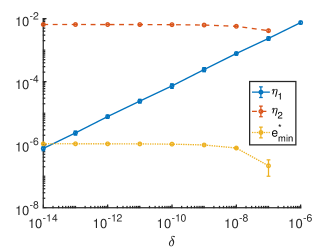
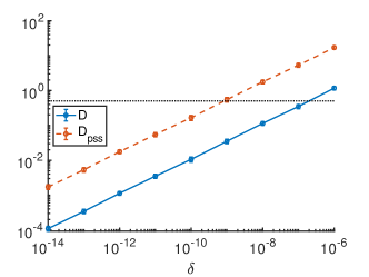
Figure 4: Characteristic lengthscales and theorem constants for the cluster of $N=10$ spheres shown in Figure 3 and discussed in Section 2.2. The cluster was randomly perturbed and then (2.11) was solved with varying tolerance parameters $\delta$ for the squared edge lengths. The graphs show the average of each quantity and estimated error bars (one standard deviation) over 20 independent perturbations at each value of $\delta$.

image	comments	theorem lengthscales
	(a) 6 vertices, 8 edges ($<$ isostatic) (see Figure 2 (B))	$\eta_{1}=0$ $\eta_{2}=0.014$, $\eta_{3}=0.0093$ $e_{\rm min}^{*}=5.7\times 10^{-6}$
	(b) 10 vertices, 23 bonds ($<$ isostatic), unit edges solved on computer to tolerance $\delta=9\times 10^{-16}$ 1 flex, 1 almost-flex, 1 almost-stress (see Figure 3)	$\eta_{1}=1.6\times 10^{-7}$ $\eta_{2}=0.0065$, $\eta_{3}=0.0044$ $e_{\rm min}^{*}=1.1\times 10^{-6}$

Table 1: Lengthscales from Theorems I-III calculated for our introductory examples (Section 2.2), using $\lambda=\lambda_{0}/2$.

4.2 A collection of examples

image	comments	theorem lengthscales
	(c) square, first-order rigid, unit height distance to other embeddings = 1.222 1.22 (fold), 2 (reflect)	$\eta_{1}=0$ $\eta_{2}=0.16$, $\eta_{3}=0.12$ $e_{\rm min}^{*}=0.12$
	(d) tetrahedron, unit edges first-order rigid distance to reflection = 1.06	$\eta_{1}=0$ $\eta_{2}=0.18$, $\eta_{3}=0.13$ $e_{\rm min}^{*}=0.15$
	(e) octahedron, unit edges first-order rigid	$\eta_{1}=0$ $\eta_{2}=0.15$, $\eta_{3}=0.11$ $e_{\rm min}^{*}=0.13$
	(f) polytetrahedron, unit edges first-order rigid	$\eta_{1}=0$ $\eta_{2}=0.078$, $\eta_{3}=0.057$ $e_{\rm min}^{*}=0.037$
	(g) isostatic (9 vertices, 21 edges), unit edges solved numerically to tolerance $\delta=9\times 10^{-16}$ 1 almost-flex, 1 almost-stress	$\eta_{1}=1.7\times 10^{-7}$ $\eta_{2}=0.0145$, $\eta_{3}=0.0099$ $e_{\rm min}^{*}=4.3\times 10^{-6}$
	(h) isostatic (6 vertices, 9 edges) prestress stable, not first-order rigid unit height	$\eta_{1}=0$ $\eta_{2}=0.13$, $\eta_{3}=0.096$ $e_{\rm min}^{*}=8.9\times 10^{-4}$
	(i) Siamese dipyramid, first embedding. 12 vertices, unit edges	$\eta_{1}=0$ $\eta_{2}=0.0064$, $\eta_{3}=0.0047$ $e_{\rm min}^{*}=3.0\times 10^{-4}$
	(j) Siamese dipyramid, second embedding. Distance to first embedding = 0.49.	$\eta_{1}=0$ $\eta_{2}=0.0068$, $\eta_{3}=0.0050$ $e_{\rm min}^{*}=3.3\times 10^{-4}$
	(k) $K_{3,4}$ (7 vertices, 12 edges), vertices on a circle globally rigid for generic $p$ this $p$ is prestress stable, not first-order rigid	$\eta_{1}=0$ $\eta_{2}=0.027$, $\eta_{3}=0.019$ $e_{\rm min}^{*}=1.3\times 10^{-5}$

Table 2: Some frameworks and their lengthscales given by Theorems I-III, calculated using $\lambda=\lambda_{0}/2$.

Table 2 shows $\eta_{1},\eta_{2},\eta_{3},e_{\rm min}^{*}$ for a collection of frameworks with different properties, that we discuss in turn.

4.2.1 Small first-order rigid frameworks

Examples (c)-(f) in Table 2 are all first-order rigid, so $\eta_{1}=0$. They have significantly larger values of $\eta_{2}$, $e_{\rm min}^{*}$ than for our introductory examples, which were not first-order rigid. For Examples (c) and (d), a two-dimensional square with a diagonal edge and a three-dimensional tetrahedron, we calculated the distance to the other embeddings of each framework (i.e. those with the same edge lengths), using the Kabsch algorithm to find the minimum distance over rigid body motions [Kabsch]. The distance is larger than $\eta_{2}$, as it must be, about 7-10 times larger for these examples.

4.2.2 An isostatic framework that is not first-order rigid

   

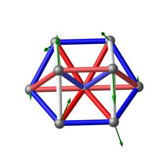
Figure 5: Left, Middle: Isostatic frameworks that are prestress stable but not first-order rigid. Each has a single infinitesimal flex (green arrows) and a single self-stress (colors on bars, where blue is positive and red is negative.) Right: $K_{3,4}$ with vertices on a circle. For generic configurtations, it has one self-stress and is globally rigid. When the vertices lie on a circle, it acquires an infinitesimal flex (green arrows) and extra self-stress. The self-stress plotted is the one that makes the framework prestress stable.

Next consider Example (g) in Table 2. This has unit edges and can be formed by putting spheres with unit diameters in contact. It has 9 vertices and 21 edges, so generically it should be first-order rigid, since the number of variables required to describe the configuration, $9\times 3=27$, equals the number of edges plus the number of rigid-body degrees of freedom. We say such a configuration is isostatic. In three dimensions a graph with $N$ vertices is isostatic when it has $3N-6$ edges, and in two dimensions it is isostatic when it has $2N-3$ edges.

However, for this particular configuration, there is an additional infinitesimal flex and self-stress; the infinitesimal flex corresponds to “twisting” the two halves of the framework relative to each other (Figure 5; see also [Kallus:2017hi].) One can argue that the framework with perfect unit edges is prestress stable; in fact, it is the smallest packing of identical spheres that is prestress stable but not first-order rigid [HolmesCerfon:2016wa].

When we represent the framework on a computer, we don’t obtain perfect unit edge lengths, so the numerically represented framework $p$ should behave like a generic configuration, and hence should be first-order rigid. Indeed, we solved (2.11) for $p$ using a tolerance of $\delta=4\epsilon\approx 9\times 10^{-16}$ and a random initial condition. The singular values of $R(p)$ were

$$1.62\times 10^{-9},\;0.61,\;0.67,\;0.78,\;0.87,\;1.02,\;1.06,\;1.14,\;1.19,\;1.30,\;1.31,\;1.35,\;1.41,\;$$

$$1.59,\;1.61,\;1.75,\;1.75,\;1.79,\;1.99,\;2.04,\;2.26.$$

The smallest singular value is $\sigma_{0}=1.62\times 10^{-9}>0$, so $p$ is first-order rigid, i.e. $\eta_{1}=0$. We applied Corollary 3.4 to calculate the other radii using this singular value, and found the outer radius to be $\eta_{2}=2.8\times 10^{-10}$, and the edge length barrier to be $e_{\rm min}^{*}=6\times 10^{-19}$, both of which are minuscule.

Can we do better, by using the almost-flex $v$ and almost-self-stress $w$ in our test? We repeated the test, choosing $\mathcal{V}=\mathcal{V}^{\sigma_{0}}$, $\mathcal{W}=\mathcal{W}^{\sigma_{0}}$ (see (3.2).) With these choices, $\eta_{1}>0$ (see Table 2 (g)), so the cluster is not provably rigid using this test. However, $D_{\rm pss}=8.6\times 10^{-5}<0.5$, so there is a nearby prestress stable cluster. The other lengthscales are $\eta_{2}=0.0145$, $e_{\rm min}^{*}=4.3\times 10^{-6}$, much bigger than they were using the first-order test above. In this case, although we know that the perturbed $p$ is rigid, from our first test, the utility of $\eta_{1}$ in the second test is to constrain the distance to nearby configurations with the same edge lengths. It could be the case – and probably is – that there is a nearby rigid configuration with the same edge lengths as the perturbed $p$, however, this nearby configuration must lie within $\eta_{1}$ of $p$; any other configuration is at least a distance of $\eta_{2}$ away, hence, much further. This example illustrates how one can choose $\mathcal{V}$, $\omega$ in different ways to prove different kinds of statements.

Example (h) in Table 2 is an isostatic cluster in two dimensions which is also prestress stable, but not first-order rigid.

4.2.3 Siamese dipyramid

Next we consider a polyhedron that is provably rigid (as a polyhedron), but, such that physical models of it “feel” flexible: they can be deformed by some finite amount, without any noticeable stretching or bending of the faces. This family of examples, called Siamese dipyramids, was introduced to the mathematics literature by Goldberg [Goldberg:1978df], and partially analyzed recently by Gorkavyy & Fesenko [Gorkavyy:2018gp]. The authors built our own physical model of a Siamese dipyramid using cardboard for the faces and scotch tape for the hinges, and it did not feel at all rigid; we could deform it significantly without noticeably bending or creasing the cardboard or ripping the hinges.

We consider Siamese dipyramids with $N=12$ nodes and unit edge lengths. There are two such examples, shown in Table 2 (i),(j), where they are plotted as frameworks, with nodes at the vertices of the polyhedron and edges at the boundaries of the faces. The two examples differ in the widths of the pac-man-like discs that make them up: in example (i), the discs are the same width, so the framework can be superimposed on itself by a reflection and a rotation by $\pi/2$. In example (j), one disc has been flattened and one has been thickened. See [Gorkavyy:2018gp] for a description of how to construct these examples.

We were curious if our theory could give insight into why these examples feel so flexible. We treated each example as a framework and calculated the various lengthscales. For example (i), call its configuration $p_{1}$, the smallest singular value of $R(p_{1})$ was $\sigma_{0}=0.0546$. Since $\sigma_{0}>0$, the framework is first-order rigid, however the singular value is significantly smaller than for a typical first-order rigid cluster. The outer radius and energy barrier are correspondingly small, $\eta_{2}=0.00638$, $e_{\rm min}^{*}=2.98\times 10^{-4}$; the outer radius in particular is much smaller than for the other first-order rigid examples we have considered, and smaller even than for some of the prestress stable sphere clusters. The constants for example (j), call its configuration $p_{2}$, were of a similar magnitude, $\sigma_{0}=0.0579$, $\eta_{2}=0.00676$, $e_{\rm min}^{*}=3.35\times 10^{-4}$. Such small outer radii and edge length barriers suggest the two embeddings could be close to each other in configuration space, and that one can deform these examples without changing the edge lengths by much.

We calculated the actual distance between the configurations (using the Kabsch algorithm to find the minimum distance over rigid body motions) and found it to be about $|p_{1}-p_{2}|\approx 0.49$, significantly larger than either value of $\eta_{2}$. Therefore, although $\eta_{2}$ may be correlated with how rigid or flexible a structure feels in practice, it does not quantitatively predict the location of other embeddings.

4.2.4 $K_{3,4}$

The example above showed that the radii in our theory can correlate with how flexible a framework “feels”, at least qualitatively. To show that feeling flexible does not always correlate with having another solution nearby, consider the graph $K_{3,4}$ in $\mathbb{R}^{2}$, See Table 2 (k). This graph is generically globally rigid: for a generic configuration, there is only one embedding of the graph in the given dimension. That $K_{3,4}$ is generically globally rigid in dimension $2$ follows from the classification of such graphs in [jacksonjordan].

However, when the vertices lie on a circle, the the $K_{3,4}$ framework acquires an extra infinitesimal flex and self-stress (Figure 5.) We took the vertices on a regular heptagon on the unit circle, and calculated the various lengthscales, see Table 2. When we perturb the vertices by small random amounts, these numbers don’t change much, however for a random perturbation the resulting framework is globally rigid. Therefore, even though its outer radius is only $\eta_{2}=0.027$, there is actually no other embedding with the same edge lengths at all.

4.3 Clusters of unit spheres

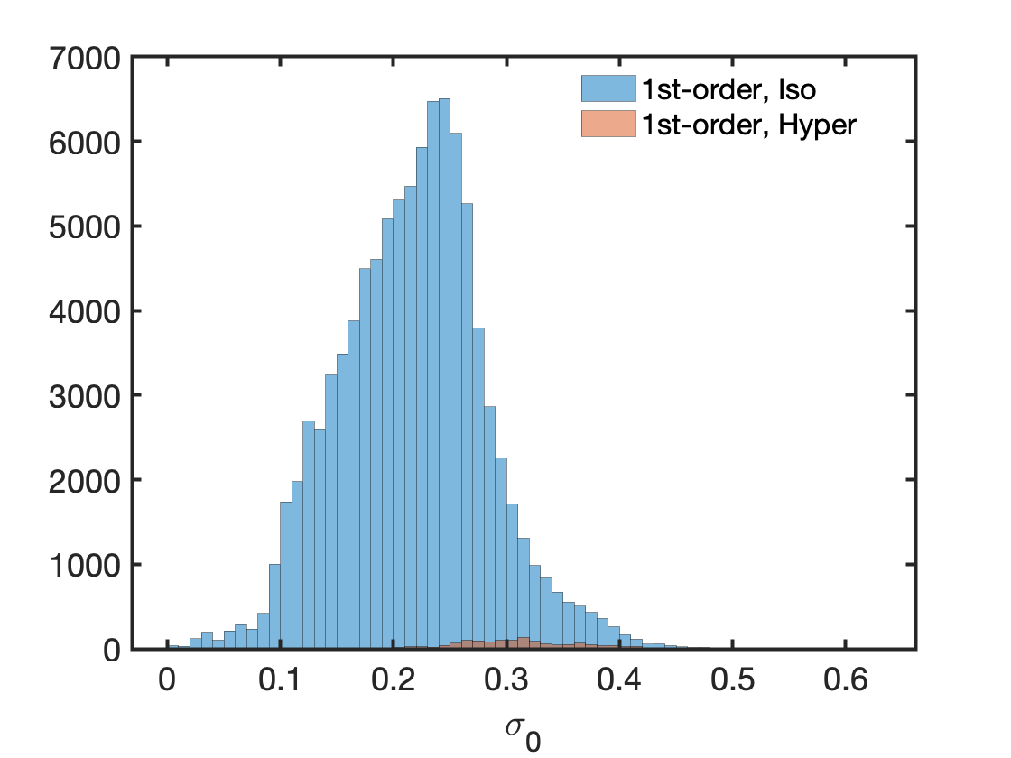
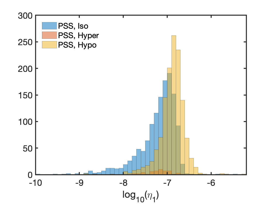
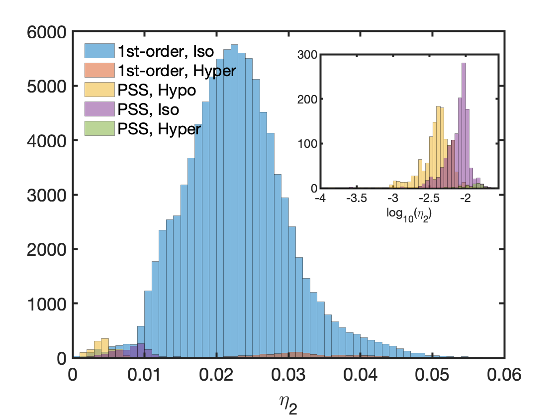
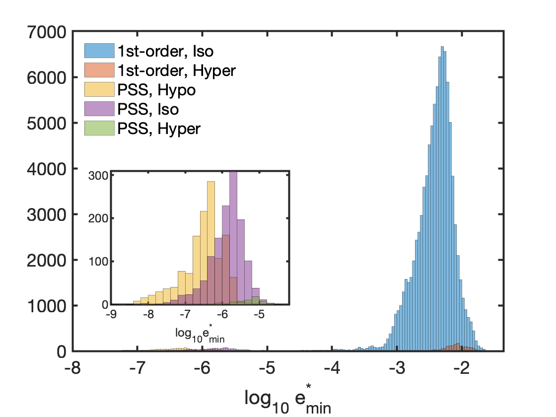
Figure 6: Lengthscales calculated for frameworks made from rigid clusters of $N=13$ identical spheres. The histograms are calculated for each type of cluster, indicated in the legends: “1st-order” (first-order rigid), “PSS” (prestress stable but not first-order rigid), “Iso” (isostatic, $3N-6$ edges), “Hyper” (hypostatic/overconstrained, $>3N-6$ edges), “Hypo” (hypostatic/underconstrained, $<3N-6$ contacts.)

For a more global picture of how the lengthscales behave for different types of frameworks, we turn to the set of rigid frameworks made from $N=13$ unit spheres in contact. A list of 98,529 such frameworks was presented in [HolmesCerfon:2016wa]; this list is thought to be nearly complete. The clusters were found by solving (2.11) numerically for different edge sets $\mathcal{E}$, using a tolerance of $\delta\approx 9\times 10^{-16}$.

Figure 6 shows a histogram of the smallest singular value $\sigma_{0}$ for all first-order rigid clusters in the dataset. The average was $0.22$ with standard deviation $0.066$, so most singular values were close to the mean. However, the largest observed value was $\sigma_{0}=0.626$, and the smallest was $\sigma_{0}=0.00106$, so even within the first-order rigid clusters, the lengthscales $\eta_{2},e_{\rm min}^{*}$ can vary by more than two orders of magnitude.

We calculated $\eta_{1},\eta_{2},e_{\rm\min}^{*}$ for all clusters, using a cutoff of $10^{-7}$ for the singular values to build $\mathcal{V},\mathcal{W}$, and choosing $\lambda=0.8\lambda_{0}$. Figure 6 shows the histograms of values, grouped by type of cluster: first-order rigid or not, and number of edges: hypostatic ($<3N-6$ edges), isostatic ($3N-6$ edges), hyperstatic ($>3N-6$ edges.) We see that hyperstatic first-order rigid clusters on average have slightly higher lengthscales than isostatic first-order rigid clusters. Non-first-order rigid clusters have values of $\eta_{2}$ that are about one to two orders of magnitude smaller than first-order rigid clusters, and values of $e_{\rm min}^{*}$ that are about 3-4 orders of magnitude smaller. Within the non-first-order rigid clusters, these values are on average slightly smaller for hypostatic clusters, and slightly larger for hyperstatic clusters. Figure 6 also shows the values of $\eta_{1}$ for the non-first-order rigid clusters, which are nonzero presumably because of numerical tolerance in solving (2.11) and because we include small singular vectors in our tests. We expect the distribution of $\eta_{1}$-values reflects the distribution of tolerances with which we solve (2.11), since our numerical solver does not produce exactly the same error for each framework.

To verify that the theorems do indeed apply, we calculated $D$, $D_{\rm pss}$ from (3.9), (3.17). The 20 largest values of $D$ were:

$$0.61,\;0.27,\;0.042,\;0.027,\;0.016,\;0.0035,\;0.0020,\;0.0018,\;0.0014,\;0.0009,\;0.0008,\;0.0007,\;$$

$$0.0006,\;0.0004,\;0.0003,\;0.0003,\;0.0003,\;0.0003,\;0.0003,\;0.0003,\ldots$$

All clusters but one had values of $D$ less than $0.5$, and therefore Theorems I, II apply. The cluster with the largest value of $D$ (cluster 45601 in the dataset), for which the theorems don’t apply, was isostatic, with one small flex $v$ and one small stress $w$ with singular value $\sigma_{0}=1.37\times 10^{-10}$, and the corresponding inner product was $v^{T}\Omega(w)v=2.03\times 10^{-4}$. Since this inner product is so tiny, the cluster had a small outer radius $\eta_{2}=1.7\times 10^{-6}$, and a large eigenvalue factor, $\bar{\mu}=14569$, which causes $D$ to be large. We computed $D$ with different values of $\lambda$, but it never fell under the threshhold for the theorems. The cluster with the second-largest $D$-value (cluster 10386) was structurally similar to the one with the largest $D$. It had a similarly large value of $\bar{\mu}$, but nevertheless its $D$-value fell under the threshhold. The authors built these clusters out of magnetic rods and ball-bearings, and they both felt very floppy.

The 20 largest values of $D_{\rm pss}$ were

$$23.7,\;10.2,\;4.5,\;1.4,\;0.48,\;0.15,\;0.11,\;0.11,\;0.092,\;0.055,\;0.050,\;0.020,\;0.018,\;$$

$$0.015,\;0.014,\;0.013,\;0.013,\;0.013,\;0.011,\;0.011,\ldots$$

All but four clusters had $D_{\rm pss}<0.5$. Therefore, Theorem IV guarantees that there is a nearby prestress stable cluster for all but these four clusters.

4.4 $L$ vs $\lambda/\lambda_{0}$

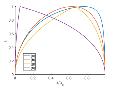
Figure 7: Lengthscale $L$ from (3.6) for examples (a),(c),(g),(h) in Table 2, as a function of $\lambda$. All curves have been scaled so their maximum value is 1.

Implementing the theory requires choosing a value $\lambda\in(0,\lambda_{0})$. Larger values of $\lambda$ lead to smaller $\eta_{1}$ (see (3.8)), which is usually desirable. However, $\lambda$ also changes the lengthscale $L$ (see (3.6)) which sets $\eta_{2},e_{\rm min}^{*}$, and it does so in a nontrivial way, since $\kappa$ also depends on $\lambda$.

We computed $L(\lambda)$ for different values of $\lambda$ for examples (a),(b),(g),(h) in Tables 1, 2. Figure 7 shows that there is no common features to the dependence. Although we must have $L(\lambda)=0$ for $\lambda=0,1$, the maximum of $L(\lambda)$ could be anywhere: for the first three examples it is somewhere in the interval $(0.6,0.8)$, but for the last example it is near $\lambda\approx 0.055$. However, $L(\lambda)$ does not change by more than about a factor of 2, within the range $\lambda\in(0.2,0.8)$. Interestingly, $L(\lambda)$ does not appear to always be a differentiable function of $\lambda$.

5 Properties of a function that is “almost” at a critical point

This section collects general results about a three-times continuously differentiable function that almost but doesn’t quite pass the second derivative test. These results will be used to prove the theorems in Section 3, but they may additionally be of independent interest.

Consider a function $H\in C^{3}(\mathbb{R}^{n})$, which we think of as an energy. The number $n$ in this section can be any dimension and does not have to be related to frameworks. Let $\mathbb{S}^{n-1}=\{v\in\mathbb{R}^{n}:|v|=1\}$ be the the unit sphere in $\mathbb{R}^{n}$. When we write $|v|=1$, we always mean $v\in\mathbb{S}^{n-1}$. Let the $k$th directional derivative in direction $v\in\mathbb{S}^{n-1}$ evaluated at point $q$ be $H^{(k)}|_{q}(v)$. This derivative can be evaluated using the chain rule as

$$H^{(k)}|_{q}(v)=\frac{d^{k}}{dt^{k}}\Bigg{|}_{t=0}H(q+tv)\,.$$ (5.1)

We sometimes write the first and second derivatives as $H^{\prime}|_{q}(v)=\nabla H(q)\cdot v$, $H^{\prime\prime}|_{q}(v)=v^{T}\nabla\nabla H(q)v$. Let $B_{r}(p)$ be the open ball of radius $r$ centered at $p$, and let $\bar{B}_{r}(p)$ be its closure.

We are interested in the setting where $|\nabla H(p)|$ is sufficiently small, $\nabla\nabla H(p)$ is sufficiently positive definite, and $|H^{\prime\prime\prime}|_{p+rv}(v)|$ is not too large for $r$ within a certain range, in a way to be defined precisely later. These assumptions imply that $p$ is “almost” a positive definite critical point, and that the third derivative doesn’t alter the positive definiteness of the Hessian in a sufficiently large ball. Under appropriate assumptions we will show three main propositions, which are stated informally as:

1. There is a radius $\eta_{1}$ such that any continuous path starting at $p$ on which the energy doesn’t increase, cannot leave the ball of radius $\eta_{1}$.

2. There is a radius $\eta_{2}>\eta_{1}$ such that the energy is positive on the annulus $(\eta_{1},\eta_{2})$. Hence, any continuous path on which the energy is not larger than $H(p)$, and such that the path contains no points in the ball of radius $\eta_{1}$, must lie entirely outside the ball of radius $\eta_{2}$.

3. A continuous path from $p$ to a point $q$ with $|q-p|=\eta$ must cross an energy barrier of at least $\Delta H_{\rm min}(\eta)$, a function of $\eta$ given explicitly from the properties of the energy.

The numbering of the propositions parallels the numbering of the theorems they will be used to prove.

Proving these propositions is technical so we do this in steps. We start by studying the behaviour of cubic univariate polynomials as the cubic coefficient varies, in Section 5.1. We show that for a polynomial $at^{3}+bt^{2}+ct$, where $b,c$ are fixed with $b>0$, and $a$ varies within limits, there is a fixed interval in $|t|$ over which the polynomial remains positive. The argument is detailed but not deep; the main theoretical tool is the quadratic formula.

Next, in Section 5.2, we study multivariate cubic functions. We use the results about cubic univariate polynomials to study the behaviour of the function along lines in different directions, to obtain an interval that is independent of direction over which the function is positive on each line. The main ideas behind the more general propositions are contained in this section, so these propositions should be possible to understand from reading this section only.

A reader undaunted by technical detail can then continue to Section LABEL:sec:energypropositionsgeneral, which considers arbitrary functions that are three-times continuously differentiable. By Taylor-expanding a function along each direction we obtain a cubic univariate polynomial with a varying cubic term, to which we may apply results from Section 5.1. The additional challenge here is that the bounds on the cubic term, and hence the estimates of the interval over which the function is positive, depend on the distance to which the Taylor expansion is valid, which in turn depend on the interval of positivity that we calculate. Therefore, we have to be careful to avoid circular definitions.

5.1 Cubic univariate function

We start with some lemmas regarding the behaviour of cubic univariate functions as the cubic term varies.

Lemma 5.1.

Consider the function

$$g(t,a)=at^{3}+bt^{2}+ct\,.$$ (5.2)

Suppose $b>0$ and $c\neq 0$, and let $t_{*}=\frac{2|c|}{b}$. Let $\bar{a}$ be a number such that $0<\bar{a}<\frac{b^{2}}{4|c|}$, and let $t_{1}^{+}(a)=\frac{b}{2|a|}(1+\sqrt{1-4|ac|/b^{2}})$. Then

$$g(t,a)>0\qquad\forall\>(t,a)\;\text{ such that }\;|t|\in[t_{*},t_{1}^{+}(\bar{a})),\quad|a|\leq\bar{a}\,,$$ (5.3)

and furthermore this interval is non-empty.

The consequences of this Lemma are illustrated in Figure 8.

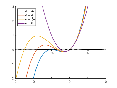
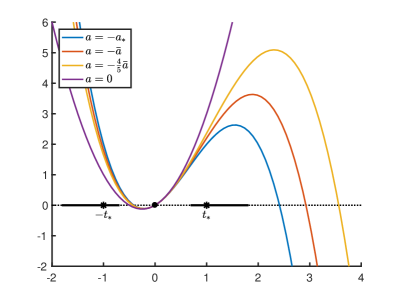
Figure 8: Example polynomials $g(t,a)=at^{3}+bt^{2}+ct$ from Lemma 5.1, with $b=2,c=1$, and varying $a$ as indicated in the legend. Here $a_{*}=b^{2}/4c$, $t_{*}=2c/b$, and we chose $\bar{a}=0.8a_{*}$. The intervals for $t$ from (5.5) where $g(t,a)$ is positive for all $-\bar{a}\leq a\leq\bar{a}$ are shown in solid black lines. Left: $0\leq a\leq a_{*}$. For $0<a<a_{*}$, both roots $t_{1}(a)$, $t_{2}(a)$ (see (5.4)) are negative and $-t_{*}$ lies between them, so the polynomials are positive in some interval surrounding $-t_{*}$, as well as for all $t>0$. Right: $-a_{*}\leq a\leq 0$. For $a<0$, the smallest root is negative and satisfies $-t_{*}<t_{1}(a)<0$, so the polynomials are positive in an interval surrounding $-t_{*}$. The largest root is positive, $t_{2}(a)>0$, and decreases as $a$ decreases but does not hit $t_{*}$ until $a$ is well below $-\bar{a}$ (even $-a_{*}$), so there is also an interval surrounding $t_{*}$ where the polynomials are positive.

Proof.

We can assume without loss of generality that $c>0$, since $g(t,a;c)=g(-t,-a;-c)$ (including here the dependence of $g$ on parameter $c$) and the conditions and statement of the lemma only depend on $|t|$, $|a|$, $|c|$.

For fixed $a$, the solutions to the cubic polynomial equation $g(t,a)=0$ are $t=\{0,t_{1}(a),t_{2}(a)\}$, where

$$t_{1}(a)=\frac{-b-\sqrt{b^{2}-4ac}}{2a},\qquad t_{2}(a)=\frac{-b+\sqrt{b^{2}-4ac}}{2a}\,.$$ (5.4)

Notice that, for $a>0$ (and $c>0$), $t_{1}^{+}(a)=|t_{1}(a)|$, so our argument will proceed by analyzing the behaviour of $t_{1}(a)$. Let $a_{*}=b^{2}/4|c|$ be the critical value of $a$ where the discriminant of the roots above vanishes. The two varying roots above are imaginary for $a>a_{*}$, real for $a\leq a_{*}$, and at the critical value they are equal, $t_{1}(a_{*})=t_{2}(a_{*})=-t_{*}$. In addition we have that for $0<a\leq a_{*}$ the varying roots are both negative, $t_{1}(a),t_{2}(a)<0$.

We will establish the following result (which is actually stronger than (5.3)):

$$g(t,a)>0\quad\text{ for }(t,a)\text{ such that }|t|\in(|t_{2}(\bar{a})|,|t_{1}(\bar{a})|),\;\;|a|\leq\bar{a}\,.$$ (5.5)

This will imply (5.3) after two short calculations. First, we must verify that $t_{*}\in(|t_{2}(\bar{a})|,|t_{1}(\bar{a})|)$. We do this by checking that $t_{1}(\bar{a})<-t_{*}<t_{2}(\bar{a})$. Differentiating the quadratic equation $at^{2}+bt+c=0$ implicitly with respect to $a$ gives $\partial_{a}t_{i}=\frac{-t^{2}_{i}}{2at_{i}+b}$. Substituting the expressions for each root gives

$$\partial_{a}t_{2}=\frac{-t_{2}^{2}}{\sqrt{b^{2}-4ac}}\quad<0,\qquad\partial_{a}t_{1}=\frac{-t_{1}^{2}}{-\sqrt{b^{2}-4ac}}\quad>0\,.$$

Since $\bar{a}<a_{*}$ we have $t_{2}(\bar{a})>t_{2}(a_{*})=-t_{*}$, $t_{1}(\bar{a})<t_{1}(a_{*})=-t_{*}$.

Second, we compute directly that $|t_{1}(\bar{a})|-t_{*}=\frac{\delta+\sqrt{\delta}}{2\bar{a}/b}$, where $\delta=1-4|\bar{a}c|/b^{2}>0$ by assumption. Therefore $\left[t_{*},t_{*}+\frac{\delta+\sqrt{\delta}}{2\bar{a}/b}\right)\subset(|t_{2}(\bar{a})|,|t_{1}(\bar{a})|)$ so result (5.5) implies result (5.3).

Now we turn to showing (5.5). Our argument follows the sketch in Figure 8. We consider the two cases $0\leq a\leq\bar{a}$ and $-\bar{a}\leq a<0$ in turn, and for each case, consider $t>0$ and $t<0$ separately.

First consider $a\geq 0$ (Figure 8, left.) When $t>0$ the cubic function $g(t,a)$ is a sum of nonnegative monomials, at least one of which is strictly positive (namely $bt^{2}>0$), so the cubic is positive, and (5.5) holds for $a\geq 0$, $t>0$. It remains to consider $t<0$. For $0<a<a_{*}$, the roots $t_{1}(a),t_{2}(a)$ are both negative and the cubic function is positive in between them, i.e. $g(t,a)>0$ for $t\in(t_{1}(a),t_{2}(a))$. Therefore since $0<\bar{a}<a_{*}$, it is true that $g(t,\bar{a})>0$ for $t\in(t_{1}(\bar{a}),t_{2}(\bar{a}))$. To extend this fixed interval to other values of $a$, we calculate $\partial_{a}g(t,a)=t^{3}<0$. Therefore $g(t,a)$ strictly increases as $a$ decreases, so $g(t,a)>0$ for $t\in(t_{1}(\bar{a}),t_{2}(\bar{a}))$ whenever $a\leq\bar{a}$, establishing (5.5) for $a\leq\bar{a}$ and $t<0$. Note the latter argument includes the case $a<0$.

Next consider $a<0$ (Figure 8, right). We have already established (5.5) for $t<0$, so we need only consider $t>0$. Since $t_{2}(a)>0$, we see that $g(t,a)>0$ for $t\in(0,t_{2}(a))$, and $g(t,a)<0$ for $t>t_{2}(a)$. By direct calculation we find $g(|t_{1}(\bar{a})|,-\bar{a})=2c>0$, so $g(t,-\bar{a})>0$ for $t\in(0,|t_{1}(\bar{a})|]$. Again we consider how $g$ varies with $a$, to find $\partial_{a}g(t,a)=t^{3}>0$ for $t>0$. Therefore $g(t,a)>0$ for all $t\in(0,|t_{1}(\bar{a})|]$, $a\geq-\bar{a}$. Therefore (5.5) holds for $a<0,t>0$ also. ∎

We need a similar lemma to deal with the case when $c=0$.

Lemma 5.2.

Consider again the cubic function (5.2) but now suppose $c=0$, in addition to $b>0$. Let $0<\bar{a}<\infty$. Then

$$g(t,a)>0\qquad\forall\>(t,a)\text{ such that }|t|\in(0,\frac{b}{\bar{a}})\,,\quad|a|\leq\bar{a}\,.$$ (5.6)

Proof.

We factor $g(t,a)=at^{2}(t+\frac{b}{a})$. As a function of $t$, this has a single root at $t=-\frac{b}{a}$ and a double root at $t=0$. If $a>0$ then $g(t,a)$ is negative for $t<-\frac{b}{a}$ and positive otherwise. If $a<0$ then $g(t,a)$ is negative for $t>-\frac{b}{a}$ and positive otherwise. If $a=0$ then $g(t,a)>0$ for all $t\neq 0$. Therefore $g(t,a)>0$ for all $|t|\in(0,b/a)$, and taking the intersection of the intervals over all $|a|\leq\bar{a}$ gives (5.6). ∎

We need one more lemma which will be used to construct an energy barrier.

Lemma 5.3.

Consider the cubic function (5.2) with $b>0$ and where $\bar{a}\geq 0$ is any nonnegative real number. Then for $t>0$,

$$g(\pm t,a)\quad\geq\quad f(t)\equiv-\bar{a}t^{3}+bt^{2}-|c|t\qquad\text{for }\;|a|\leq\bar{a}\,.$$ (5.7)

Proof.

For $a\geq-\bar{a}$,

$$g(t,a)-f(t)=(a+\bar{a})t^{3}+(c+|c|)t\;\;\geq\;\;0\,.$$

For $a\leq\bar{a}$,

$$g(-t,a)-f(t)=(\bar{a}-a)t^{3}+(|c|-c)t\;\;\geq\;\;0\,.$$

Therefore for $|a|\leq\bar{a}$, both $g(t,a)\geq f(t)$, and $g(-t,a)\geq f(t)$, hold. ∎

5.2 Cubic energy function