Towards Online Observability-Aware Trajectory Optimization for Landmark-based Estimators

Abstract

As autonomous systems increasingly rely on onboard sensing for localization and perception, the parallel tasks of motion planning and state estimation become more strongly coupled. This coupling is well-captured by augmenting the planning objective with a posterior-covariance penalty – however, prediction of the estimator covariance is challenging when the observation model depends on unknown landmarks, as is the case in Simultaneous Localization and Mapping (SLAM). This paper addresses these challenges in the case of landmark- and SLAM-based estimators, enabling efficient prediction (and ultimately minimization) of this performance metric. First, we provide an interval-based filtering approximation of the SLAM inference process which allows for recursive propagation of the ego-covariance while avoiding the quadratic complexity of explicitly tracking landmark uncertainty. Secondly, we introduce a Lie-derivative measurement bundling scheme that simplifies the recursive “bundled” update, representing significant computational savings for high-rate sensors such as cameras. Finally, we identify a large class of measurement models (which includes orthographic camera projection) for which the contributions from each landmark can be directly combined, making evaluation of the information gained at each timestep (nearly) independent of the number of landmarks. This also enables the generalization from finite sets of landmarks $\{\ell^{(n)}\}$ to distributions, foregoing the need for fully-specified linearization points at planning time and allowing for new landmarks to be anticipated. Taken together, these contributions allow SLAM performance to be accurately and efficiently predicted, paving the way for online, observability-aware trajectory optimization in unknown space.

1 Introduction

In the last decade, significant progress has been made to enable basic autonomy for low-SWaP (Size, Weight, and Power) systems. Thanks to recent algorithmic advances, such systems can navigate purely from onboard sensors and avoid dependence on dedicated infrastructure such as GPS or motion-capture, allowing operation in a wider range of environments. However, commonly-used sensors such as IMUs, laser scanners, and cameras have nonlinear observation models and/or limited field-of-view (FoV), and therefore the observability of the estimated state will fundamentally depend on the system trajectory. Furthermore, these sensors can have time-varying latent parameters (e.g., IMU biases, rigid-body calibrations) and environmental dependencies (e.g., the presence or absence of high-gradient corner features). Thus, even with a good initialization point, estimation quality can degrade to catastrophic levels if the chosen trajectory or environment does not provide sufficient information.

In this paper, we are interested in discovering well-observable motions accounting for the (possibly latent) distribution of landmarks over receding time-horizons. This motivates continuous optimization techniques leveraging a full-DoF system model, and efficient evaluation requires a compact representation of the SLAM inference process. In focusing on receding time-horizons, we are willing to neglect certain aspects of SLAM such as global loop closure in favor of computational efficiency and applicability to real-world scenarios where the map is not fully known at planning time.

When formulating the uncertainty-aware planning problem, we follow the common approach [21, 3, 24, 25, 11, 27] of representing uncertainty as a Gaussian distribution about a nominal trajectory. This representation is deterministic and compactly parameterizable, and is therefore amenable to optimization based on trajectory sampling [21, 3, 24], motion-primitives [9, 14, 8, 27], or continuous optimization [11, 25]. Of these, sampling-based approaches are not well-suited for systems with more than a few degrees of freedom, and motion-primitive solutions do not address the fundamental issue of ensuring trajectories are well-observable in the first place. In the space of continuous trajectory optimization, existing approaches have only been demonstrated with relatively simple sensor models [20, 22, 25] or scale poorly to large numbers of landmarks [11].

In order to avoid the computational challenges associated with explicit covariance prediction and minimization, heuristic approaches maximize an observability or (in the case of landmark-based systems) visibility metric. For example, [5, 16, 1] identify and enumerate non-observable configurations to hand-design a discrete set of “well-observable” maneuvers for use in online planning. More recently, [19] leverages a reinforcement learning framework to select a sequence of primitive maneuvers in a manual calibration routine. Working from a continuous optimization framework, [15, 20] design trajectories which maximize observability metrics based on the Local Observability Gramian (LOG). For landmark-based systems with limited FoV (e.g., visual SLAM), explicit visibility-based metrics have been used by [10] and [18] in real-time planning frameworks, with some success. However, LOG and visibility objectives are ultimately heuristic and therefore may select high-energy (expensive) trajectories with little corresponding estimation improvement [22].

Nevertheless, direct posterior-covariance minimization is challenging, particularly in the case of SLAM. Landmark-based systems such as visual SLAM can estimate tens or hundreds of landmarks simultaneously, and linearization points of to-be-discovered landmarks are generally unknown at planning time. Besides having to compute and accumulate the contribution from each of these landmarks (linear complexity), explicit representation of the belief state requires either reasoning over random factor graphs or maintaining the joint covariance matrix over the ego-state and map, both of which are intractable in online application. Furthermore, high-rate sensors such as cameras can produce many measurements over the time-horizon in consideration, furthermore contributing to the complexity of direct covariance analysis. While [14] and [8] introduce some sparsification and incremental-update techniques to partially mitigate the cost of graph-based evaluation with large maps, they require known landmark linearization points and are applicable only in the case of finite action sets.

1.1 Contributions

In this work, we address these challenges to enable efficient posterior-covariance prediction and minimization for a general class of landmark-based observation models.

• Measurement bundling: To avoid the prohibitive complexity of forward-simulating the SLAM estimation process during motion planning, Section 3 describes a compact, filtering-based approximation that avoids representation of the landmark uncertainty entirely. We refer to this simplified framework as the Structureless Interval Information Filter (SIIF), as it “bundles” measurements according to pre-specified time intervals and marginalizes out the uncertain map state from each “interval update.”

• A Lie-Taylor update approximation: The exact or “explicit” form of the SIIF update represents the full history of discrete-time process noise within the interval and requires multiple rounds of state integration, resulting in non-trivial computation. To simplify implementation and reduce computation, Section 4.2 introduces an approximate form of the interval update based on continuous-time Lie derivatives. This provides significant computational speedups (particularly in the case of high-rate sensors like cameras) while preserving the observability characteristics of the system.

• Handling large numbers of unknown landmarks: In general, the information contribution from each landmark must be computed individually, rendering the SIIF update expensive when landmarks number in the hundreds and ill-posed when linearization points are unavailable. Fortunately, we identify a convenient (and useful) class of sensor models for which the total information against a landmark distribution can be computed directly. From a purely computational perspective, this facilitates scaling to large clouds of hundreds or even thousands of landmarks, and ultimately allows planning against predictive models of feature density in the environment. As compared to [28], which only applies to a particular observation and visibility model of known landmarks, our decomposition applies to a much more general class of models which includes orthographic camera projection.

In Section 6 we numerically validate our measurement bundling approximation, demonstrating significant computational improvement with low approximation error. Moreover, we evaluate our full trajectory generation pipeline over a large number of random trials, demonstrating more effective estimation improvement than heuristic methods (in a Pareto sense). Although a fully online planning implementation is still in-work, the improvements and results herein suggest that real-time performance should be attainable.

2 Preliminaries

We assume the system state $x$ lies on an $n_{x}$-dimensional manifold $X$ with dynamics given by the stochastic ODE

$$\mathop{}\!\mathrm{d}x(t)=f\big{(}x(t),u(t)\big{)}\mathop{}\!\mathrm{d}t+\tens{G}_{c}\big{(}x(t),u(t)\big{)}\mathop{}\!\mathrm{d}\vec{w}(t).$$ (1)

The input $u(t)$ is confined to a set $\mathcal{U}$, and $\vec{w}(\cdot)$ is a standard Brownian noise process. We assume measurements are acquired by a collection of homogeneous sensors

$${\vec{z}^{(n)}}=h(x;\ell^{(n)})+{\vec{\nu}^{(n)}}\quad\in\mathbb{R}^{m},$$ (2)

each corrupted by an independent Gaussian noise ${\vec{\nu}^{(n)}}$ and parameterized by a latent environmental variable $\ell^{(n)}$ (i.e., a landmark). We assume that these measurements are acquired synchronously with frequency $1/\Delta t$. Without loss of generality, each ${\vec{\nu}^{(n)}}$ is assumed to have identity covariance.

We are interested in the setting where state $x(t)$ and landmarks $\{\ell^{(n)}\}$ are all uncertain, and that the system controller must operate from an estimated state $\vec{\hat{x}}(t)$. It is worth noting that our framework avoids making any implementation-specific assumptions with regard to this “estimator,” aside from the fact that it is constrained to operate as a function of the observation history and initializes from a Gaussian prior with mean $\vec{\hat{x}}_{0}$ and covariance $\tens{P}_{0}$. For the purposes of planning well-observable trajectories, this paper will apply a local Linear-Time-Varying (LTV) assumption which simplifies computation of the “optimal” error covariance as a deterministic function of the underlying trajectory. It is worth emphasizing that under this framework, the posterior error covariance $\tens{P}(T)$ reflects the intrinsic (local) observability properties of the trajectory in implementation-agnostic way.

2.1 Local Linear-Time-Varying (LTV) dynamics

Let $\big{(}x(\cdot),u(\cdot)\big{)}$ define a nominal (noise-free) state/control trajectory pair, that is it obeys $\dot{x}=f(x,u)$. The small-perturbation dynamics can then be approximated by linearizing $f$ and $h$ about $(x,u)$ and the landmark linearization points $\{\ell^{(n)}\}$. This gives a stochastic LTV system

$$\mathop{}\!\mathrm{d}{\vec{\delta x}}(t) \approx\Big{(}\tens{A}_{c}(t){\vec{\delta x}}(t)+\tens{B}_{c}(t){\vec{\delta u}}(t)\Big{)}\mathop{}\!\mathrm{d}t+\tens{G}_{c}(t)\mathop{}\!\mathrm{d}\vec{w}(t)$$ (3a)

$${\vec{\delta}{\vec{z}^{(n)}}}(t) \approx\tens{H}\big{(}x(t);\ell^{(n)}\big{)}{\vec{\delta x}}(t)+\tens{L}\big{(}x(t);\ell^{(n)}\big{)}{\vec{\delta l}^{(n)}}+{\vec{\nu}^{(n)}}(t)$$ (3b)

where we have the dropped the explicit dependence on the linearization point $\big{(}x(t),u(t),\ell^{(n)}\big{)}$ for clarity. Note that the local observation model (3b) depends not only on the state deviation ${\vec{\delta x}}(t)$ but also the deviation of the landmark ${\vec{\delta l}^{(n)}}$.

The estimator error covariance $\tens{P}(t)$ is defined with respect to an assumed error state $\vec{e}(t)=\vec{\hat{x}}(t)\boxminus x(t)$, where the $\boxminus$ operator reflects a generalized “difference” operator on the manifold $X$. Crucially, for reasons that will be elaborated later, we specifically avoid representing the landmark deviations in $\vec{e}(t)$, which would have quadratic complexity implications on the matrix $\tens{P}(t)$. This will be accomplished via a marginalization approach similar in spirit to the MSCKF [17], and is motivated by the fact that we seek an efficient proxy for estimator performance (capturing “observability” as a function of a trajectory) rather than an actual estimator implementation.

2.2 Trajectory Optimization

This paper focuses on deterministic, continuous optimal control problems of the form

$$\min_{u(\cdot)} \qquad J_{c}(u)+\lambda J_{\text{obs}}(u)$$ (4)

subject to: $$\qquad\dot{x}(t)=f\big{(}x(t),u(t)\big{)}\qquad x(0)=x_{0}$$ (5)

$$\qquad u(t)\in\mathcal{U}\qquad x(t)\in X_{\text{safe}}$$

where we have augmented a “conventional” cost functional $J_{c}$, representing a min-energy or min-time objective, with auxiliary penalty $J_{\text{obs}}$ capturing the effects of uncertainty. Note that the dynamics constraint (5) is defined via a noise-free, nominal model.

Note that irrespective of the choice of $J_{\text{obs}}$, the presence of nonlinear dynamics is generally sufficient to imply that only numeric, local solutions are available in practice. Thus, choice of a non-convex $J_{\text{obs}}$ does not usually make (4) fundamentally harder to solve. However, it is critical that $J_{\text{obs}}$ be differentiable so that gradient-based methods can still be applied, and that such gradients can be efficiently computed.

2.3 Choices of Uncertainty Metric $J_{\text{obs}}$

At a high level, a good choice of uncertainty term $J_{\text{obs}}$ should produce a multi-objective optimization which smoothly and efficiently trades expedience (captured by $J_{c}$) for estimation performance. A number of choices for $J_{\text{obs}}$ have been proposed in the literature, but they generally fall into one of three classes.

2.3.1 Maximizing landmark visibility:

A common heuristic in the case of landmark-based estimators (i.e. visual-inertial odometry) is to maximize some visibility metric [10, 18]. While this encourages onboard sensors to be pointed towards informative parts of the environment, it does not explicitly capture the observability properties of the system.

2.3.2 Maximizing the Observability Gramian or Fisher-information:

From a control-theoretic perspective, [15] and [20] propose maximization of metrics based on the Local Observability Gramian (LOG). The LOG is equivalent to the Fisher information up to a constant scaling. Because $\tens{\Lambda}\succeq 0$ is singular for trajectories about which the system is locally unobservable, [15] and [20] propose maximization of the smallest eigenvalue $s_{1}(\tens{\Lambda})\geq 0$.

However, there are some challenges to direct maximization. Each row and column of $\tens{\Lambda}$ corresponds to a different estimated state variable, and can refer to quantities as varied as positions, velocities, and IMU biases. Maximization of individual sub-matrices (e.g., the position block) as proposed by [20] maintains consistent units of measurement, but is information-theoretically equivalent to conditioning on all other states (treating them all as known) and fundamentally neglects key observability properties of the system. Joint maximization, on the other hand, requires some scaling method; two different statistical approaches are presented in [20] and [19]. Ultimately, direct maximization of $\tens{\Lambda}$ is heuristic and, as pointed out by [22], can produce expensive trajectories (with respect to $J_{c}$) that yield little improvement in actual estimation error.

2.3.3 Minimizing posterior covariance:

Following a number of existing works [21, 24], we propose minimization of the posterior estimator covariance $\tens{P}(t)\succeq 0$. In contrast to the Fisher information or LOG, the posterior covariance of the EKF captures uncertainty in both the system dynamics and sensing. Furthermore, sub-blocks of $\tens{P}_{k}$ represent the marginal covariances over those variables, capturing the effects of all other unknown states. Minimization over the trajectory allows the optimization to smoothly trade-off between minimizing uncertainty and conventional planning costs, even to the extent of allowing $\tens{\Lambda}_{k}$ singular at some instances. Moreover, this trade-off can naturally take into account the initial uncertainty $\tens{P}_{0}$.

In particular, if $\tens{Y}$ is chosen to select the sub-block of $\tens{P}_{k}$ corresponding to the estimated position ${}^{w}\vec{\hat{p}}_{k}$, then

$$J_{\text{obs}}(u)\triangleq\sum_{{\bar{k}}=1}^{{\bar{K}}}\mathrm{tr}\mathop{}\!\big{(}\tens{Y}\tens{P}_{\bar{k}}\tens{Y}^{\top}\big{)}=\sum_{{\bar{k}}=1}^{\bar{K}}\mathbb{E}\mathop{}\!||{}^{w}\vec{\hat{p}}_{\bar{k}}-{}^{w}\vec{p}_{\bar{k}}||_{2}^{2}.$$ (6)

That is, this choice of $J_{\text{obs}}$ explicitly minimizes the mean-squared estimator error over position (with well-defined units of m²). In a sense, minimizing the posterior covariance is similar to maximizing $\tens{\Lambda}$, but warped and scaled correctly by the dynamics and prior uncertainty of the system.

3 Approximating the SLAM Estimation Process

In order to solve the optimal control problem over the continuum of possible control inputs, we require an efficient means of computing posterior covariance as a function of a nominal trajectory. This section outlines our approximation and how it differs from existing work, and introduces the proposed Structureless Interval Information Filter (SIIF) framework that will be elaborated in the rest of the paper.

A key aim of this paper is to efficiently approximate the covariance dynamics corresponding to the locally-LTV system (3), in order to enable observability-aware trajectory generation. Note that, if it were not for the dependence on the environmental features $\{\ell^{(n)}\}$, these dynamics would be given by the familiar Kalman Filter (KF) equations. While the point (mean) state estimate evolves according to the realized observations (and is therefore unknown at planning time), the error covariance evolves deterministically as a function of the underlying, linearizing trajectory .

3.1 Challenges in the SLAM case

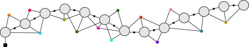
(a) Typical SLAM factor graph

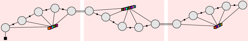
(b) Our Structureless Interval Filter (SIIF) approximation

Figure 1: The original SLAM factor graph includes both pose and landmark variables over the trajectory, and its structure depends on FoV constraints and (potentially unknown) landmark locations. Even when the graph is fully known at planning time, exact computation of the posterior covariance is expensive, prohibiting the multiple evaluations required for online observability-aware planning. In contrast, our SIIF approximation breaks up the trajectory into time intervals and discards inter-interval loop closures, Then connectivity can be generalized by enforcing a landmark visibility weighting within the Jacobians themselves, and landmarks can then be marginalized out over each interval. This produces a compressed sequence of structureless, “bundled” measurements allowing the covariance to be propagated efficiently according to a recursive update law, as described in Section 4.

When sensors do depend on landmarks as in (2) – the setting assumed in this paper – predicting and optimizing estimator performance over trajectories becomes fundamentally more challenging. This is because the locations of landmarks are usually uncertain (the case assumed in SLAM), and indeed often completely unknown at planning time. Of course, a number of filtering approaches such as MonoSLAM [6] and ROVIO [2] account for landmark uncertainty by including the landmark error $\{{\vec{\delta l}^{(n)}}\}$ in the error state. However, this augmentation comes at a quadratic cost with the number of landmarks and is clearly intractable when numerous rapid evaluations are required for online optimization.

A popular alternative to filtering approaches instead views the estimation problem over the entire trajectory (i.e., in batch) as a factor graph, as in Fig. 1a. In a factor graph, variable nodes represent unknowns such as robot poses and landmark locations, and factor nodes represent measurements or priors. Significant work over the last decade has produced efficient estimation techniques over factor graphs, particularly leveraging sparsity [7, 12, 8, 14] to minimize computation. However, these techniques assume full knowledge of the graph, which ultimately depends on sensor field-of-view (FoV) and therefore on both the trajectory and locations of landmarks. When landmark locations are unknown, observability-aware trajectory optimization could then be viewed as an optimization over (random) graphs – a clearly unsuitable formulation in the context of online, continuous trajectory optimization .

3.2 The SIIF Formulation

To avoid the complexities of the graph-theoretic view, we adopt a “structureless” filtering formulation similar to the MSCKF [17]. In order to properly account for landmark uncertainty across timesteps without augmenting the error state vector, we develop a bundled filter update over time intervals. As illustrated in Fig. 1b, this can be visualized by explicitly partitioning the factor graph according to these a priori time intervals and then marginalizing the landmarks. The resulting estimation problem can be solved algorithmically via a recursive, bundled updating procedure we refer to as the interval filter.

It is crucial to note here that for the purpose of optimizing observability-aware trajectories, we are only concerned with efficiently representing the estimation process, and are not actually producing an estimate. To accomplish this we only require a (deterministic) model of covariance propagation over time and do not need to produce an actual state estimate (as this would require access to “future” observations). Moreover, the interval filtering model proposed in Fig. 1b is clearly sub-optimal, as it decouples inter-interval connections and loop closures (thus discarding information). Nevertheless, it will be seen that the computational and algorithmic benefits of this approximation are significant, and the resulting model is sufficient to capture the “short-horizon” observability characteristics of SLAM for the purposes of planning. Furthermore, this will enable generalization to the case where landmark locations are only known in a distributional sense, and thus estimator performance can be predicted well beyond known space.

The remainder of this paper details how this interval filter is propagated, how landmarks can be anticipated into the future, and how the resulting covariance estimate can be used in planning. Section 4 describes how measurements over each interval can be bundled and the landmarks marginalized out. Additionally, it proposes a Lie-derivative-based approximation which greatly simplifies Jacobian formation in the case of high-rate sensors such as cameras. Section 5 defines a privileged class of sensor models (those with Jacobians affine in the landmark $\vec{l}^{(n)}$), and describes how information contributions from all landmarks can be aggregated directly without explicit (linear-time) summation. Besides expediting computation, this allows for generalization to distributions of landmarks, allowing natural reasoning about where new landmarks might be discovered. Finally, Section 6 gives some preliminary planning results demonstrating that significant covariance reduction can indeed be achieved for popular systems such as quadrotor-equipped VIO, and that heuristic alternatives are often ineffective.

4 The SIIF Update

For high-rate sensors such as cameras, simulation of the EKF update (and subsequent gradient back-propagation) at measurement rate can be intractable for real-time planning. For this reason, we propose a computationally-efficient method to “bundle” multiple high-rate measurements into a single update. In contrast to the traditional Kalman Filter, which proceeds one measurement timestep at a time, our approximate filter operates on larger “chunks” of time, incorporating batches of observations according to user-specified interval length $K>1$. The overall planning horizon is comprised of ${\bar{K}}$ such intervals, accounting for a total of $K{\bar{K}}$ individual measurement timesteps. Besides reducing the total number of “updates” required to model high-rate sensors, this allows for landmark uncertainty to be marginalized away within each interval, avoiding the need to track landmark uncertainty across intervals. This marginalization is information-theoretically “lossy” but yields significant computational and algorithmic benefits while capturing the fundamental observability characteristics of the system, particularly over short horizons.

Without loss of generality, assume that measurements are collected every $\Delta t$ seconds and consider a single time interval $[0,T=K\Delta t]$ for some $K>1$. Let $\mathcal{T}=\{t_{0}=0,t_{1},t_{2},\ldots,t_{k}=T\}$ refer to the set of corresponding $(K+1)$ evenly-spaced timesteps. Following a conventional filtering paradigm, assume we are given a prior estimate $\vec{\hat{x}}_{0}$ with corresponding error $\vec{e}_{0}\sim\mathcal{N}(\vec{0},\tens{P}_{0}=\tens{S}_{0}^{-1})$. From here, we seek an update equation or algorithm that ingests the proceeding batch of linearized observations $\big{(}{\vec{\tilde{z}}_{1}^{(n)}},{\vec{\tilde{z}}_{2}^{(n)}},\ldots,{\vec{\tilde{z}}_{K}^{(n)}}\big{)}$ and outputs a posterior estimate $\vec{\hat{x}}_{K}$. However, it is worth pointing out that for the purposes of planning, we do not actually need to do inference (that is, compute the point estimate $\vec{\hat{x}}_{K}$). Rather, in this paper we focus solely on the covariance update, which as discussed in the previous section can indeed be considered a deterministic function of the nominal trajectory.

From the continuous-time LTV dynamics (3), we can produce a discrete-time error dynamics model

$$\vec{e}_{k+1} =\underbrace{\big{(}\tens{I}+\Delta t\tens{A}_{c}(x_{k},u_{k})\big{)}}_{\triangleq\tens{A}_{k}}\vec{e}_{k}+\underbrace{\sqrt{\Delta t}\tens{G}_{c}(x_{k},u_{k})}_{\triangleq\tens{G}_{k}}\vec{w}_{k}$$ (7)

$${\vec{\tilde{z}}_{k}^{(n)}} =\sigma(x_{k},\ell^{(n)})\underbrace{\tens{H}(x_{k};\ell^{(n)})}_{\triangleq\tens{H}_{k}^{(n)}}\vec{e}_{k}+\underbrace{\tens{L}(x_{k};\ell^{(n)})}_{\triangleq\tens{L}_{k}^{(n)}}\vec{\tilde{l}}^{({n})}+{\vec{\nu}_{k}^{(n)}}$$ (8)

where $\sigma(x;\ell^{(n)})\in[0,1]$ indicates the “visibility” of landmark $\ell^{(n)}$ from state $x$. When $\sigma(x;\ell^{(n)})=0$ (i.e., the landmark is out of view), and no information is obtained. Under evaluation, $\sigma$ takes “hard” values of $\{0,1\}$, but during optimization it will be useful to instead apply a smooth approximation as in [28]. A candidate choice of $\sigma$ tailored for use with pinhole camera models is given in Appendix A.

For the purposes of our interval filtering approximation, it will be useful to assume that visibility is constant over each interval – that is, we will replace (8) with

$${\vec{\tilde{z}}_{k}^{(n)}}\approx\sigma(x_{0},\ell^{(n)})\underbrace{\tens{H}(x_{k};\ell^{(n)})}_{\triangleq\tens{H}_{k}^{(n)}}\vec{e}_{k}+\underbrace{\tens{L}(x_{k};\ell^{(n)})}_{\triangleq\tens{L}_{k}^{(n)}}\vec{\tilde{l}}^{({n})}+{\vec{\nu}_{k}^{(n)}}.$$ (9)

Though clearly approximate, this will allow significant computational speedup and is intuitively reasonable for short interval lengths.

4.1 Overview: Update in information space

From (7) it is straightforward to write the error state trajectory over the interval

$$\begin{bmatrix}\vec{e}_{1}\\ \vec{e}_{2}\\ \vdots\\ \vec{e}_{K}\end{bmatrix}=\underbrace{\begin{bmatrix}\tens{A}_{0}\\ \tens{\Phi}^{1}_{0}\\ \vdots\\ \tens{\Phi}^{K-1}_{0}\end{bmatrix}}_{\triangleq\mathcal{A}(x_{0},u_{0})}\vec{e}_{0}+\underbrace{\begin{bmatrix}\tens{G}_{0}&&&&\\ \tens{A}_{1}\tens{G}_{0}&\tens{G}_{1}&&&&\\ \tens{\Phi}^{2}_{1}\tens{G}_{0}&\tens{A}_{2}\tens{G}_{1}&\tens{G}_{2}&&&\\ \vdots&\vdots&\vdots&\ddots&\end{bmatrix}}_{\triangleq\mathcal{G}(x_{0},u_{0})}\underbrace{\begin{bmatrix}\vec{w}_{0}\\ \vec{w}_{1}\\ \vec{w}_{2}\\ \vdots\\ \vec{w}_{K-1}\end{bmatrix}}_{\triangleq\mathcal{W}}$$ (10)

where the error state transition matrix $\tens{\Phi}^{k_{1}}_{k_{2}}\triangleq\tens{\Phi}(t_{k_{1}},t_{k_{2}})\approx\tens{A}_{k_{1}}\tens{A}_{k_{1}-1}\ldots\tens{A}_{k_{2}}$.

Using (9), the corresponding measurement innovations for each landmark $\ell^{(n)}$ can be written

$$\begin{bmatrix}{\vec{\tilde{z}}_{1}^{(n)}}\\ {\vec{\tilde{z}}_{2}^{(n)}}\\ \vdots\\ {\vec{\tilde{z}}_{K}^{(n)}}\end{bmatrix} =\sigma(x_{0};\ell^{(n)})\Bigg{(}\underbrace{\texttt{blkdiag}\!\begin{bmatrix}\tens{H}_{1}^{(i)}\\ \tens{H}_{2}^{(i)}\\ \vdots\\ \tens{H}_{K}^{(i)}\end{bmatrix}}_{\triangleq\mathcal{H}(x_{0},u_{0};\ell^{(n)})}\begin{bmatrix}\vec{e}_{1}\\ \vec{e}_{2}\\ \vdots\\ \vec{e}_{K}\end{bmatrix}+\underbrace{\begin{bmatrix}\tens{L}_{1}^{(i)}\\ \tens{L}_{2}^{(i)}\\ \vdots\\ \tens{L}_{K}^{(i)}\end{bmatrix}}_{\triangleq\mathcal{L}(x_{0},u_{0};\ell^{(n)})}\vec{\tilde{l}}^{({n})}\Bigg{)}+\underbrace{\begin{bmatrix}{\vec{\nu}_{1}^{(n)}}\\ {\vec{\nu}_{2}^{(n)}}\\ \vdots\\ {\vec{\nu}_{K}^{(n)}}\end{bmatrix}}_{\triangleq\mathcal{V}^{({n})}}$$ (11)

$$=\sigma_{0}^{(n)}\Big{(}\mathcal{H}^{({n})}\begin{bmatrix}\mathcal{A}&\mathcal{G}\end{bmatrix}\begin{bmatrix}\vec{e}_{0}\\ \mathcal{W}\end{bmatrix}+\mathcal{L}^{({n})}\vec{\tilde{l}}^{({n})}\Big{)}+\mathcal{V}^{({n})}$$ (12)

where for clarity we’ve introduced the shorthand $\mathcal{H}^{({n})}=\mathcal{H}(x_{0},u_{0};\ell^{(n)})$ and $\mathcal{L}^{({n})}(x_{0},u_{0};\ell^{(n)})$ and otherwise suppressed the $(x_{0},u_{0})$ dependence.

As shown by Mourikis et al.[17], the landmark error $\vec{\tilde{l}}^{({n})}$ can be marginalized out by computing the left-nullspace matrix ${\mathcal{Q}^{({n})}}$ subject to

$${\mathcal{Q}^{({n})}}^{\top}\mathcal{L}^{({n})}=\tens{0}\quad\text{ and }\quad{\mathcal{Q}^{({n})}}^{\top}{\mathcal{Q}^{({n})}}=\tens{I}.$$ (13)

Then left-multiplication of (12) by ${\mathcal{Q}^{({n})}}^{\top}$ produces a marginalized innovation

$$\mathcal{Z}^{({n})}_{\text{exp}}\triangleq\sigma_{0}^{(n)}\underbrace{{\mathcal{Q}^{({n})}}^{\top}\mathcal{H}^{({n})}\begin{bmatrix}\mathcal{A}&\mathcal{G}\end{bmatrix}}_{\triangleq\overline{\mathcal{H}}_{\text{exp}}(x_{0},u_{0};\ell^{(n)})}\begin{bmatrix}\vec{e}_{0}\\ \mathcal{W}\end{bmatrix}+{\mathcal{Q}^{({n})}}^{\top}\mathcal{V}^{({n})}$$ (14)

(14) allows us to interpret the sequence of measurements corresponding to $\ell^{(n)}$ as a large, joint measurement over $\vec{e}_{0}$ and $\mathcal{W}$. Note that by construction, the ${\mathcal{Q}^{({n})}}^{\top}\mathcal{V}^{({n})}$ term refers to an i.i.d. additive noise with unit covariance. This perspective allows the joint information over $(\vec{e}_{0},\mathcal{W})$ to be combined additively as

$$\tens{\Lambda}_{0}(x_{0},u_{0})=\underbrace{\begin{bmatrix}\tens{S}_{0}&\tens{0}\\ \tens{0}&\tens{I}\end{bmatrix}}_{\triangleq\tens{\Lambda}_{0}^{\text{prior}}}+\sum_{n=1}^{N}\sigma_{0}^{(n),2}\,\underbrace{\overline{\mathcal{H}}_{\text{exp}}(x_{0},u_{0};\ell^{(n)})^{\top}\overline{\mathcal{H}}_{\text{exp}}(x_{0},u_{0};\ell^{(n)})}_{\triangleq\tens{\Lambda}_{0}^{\mathcal{Z}}(x_{0},u_{0};\ell^{(n)})}.$$ (15)

In (15) we recall the functional dependence of the underlying Jacobians and the visibility score $\sigma$ on the nominal trajectory over the interval, which in turn is a deterministic function of $x_{0}$ and the control over the interval $u_{0}$. Furthermore, note that the information matrices involved are defined jointly over a single error state $\vec{e}_{0}$ and the interval-length process noise $\mathcal{W}$.

While (15) gives a convenient form for the information “update”, we still must propagate the uncertainty from initial state $\vec{e}_{0}$ to the error state at the end of the interval $\vec{e}_{K}$ and marginalize out the nuisance variable $\mathcal{W}$. Fortunately, we have from (7) we have

$$\begin{bmatrix}\vec{e}_{K}\\ \mathcal{W}\end{bmatrix}=\underbrace{\begin{bmatrix}\tens{\Phi}^{K}_{0}&\tens{\Phi}^{K}_{1}\tens{G}_{0}&\tens{\Phi}^{K}_{2}\tens{G}_{1}&\ldots&\tens{G}_{K-1}\\ \tens{0}&&\tens{I}&&\end{bmatrix}}_{\triangleq\tens{M}(x_{0},u_{0})}\begin{bmatrix}\vec{e}_{0}\\ \mathcal{W}\end{bmatrix}$$

and it is then straightforward to verify that

$$\tens{\Lambda}_{K}=\tens{M}^{-\top}\tens{\Lambda}_{0}\tens{M}^{-1}.$$ (16)

Note that inversion of $\tens{M}$ is possible so long as $\tens{\Phi}^{K}_{0}$ is invertible (a very mild condition), and can be significantly accelerated by leveraging the block sparsity pattern. From $\tens{\Lambda}_{K}$, the marginal covariance over $\vec{e}_{k}$ can be extracted via Schur complement

$$\tens{S}_{K}=[\tens{\Lambda}_{K}]_{\vec{e}_{K},\vec{e}_{K}}-[\tens{\Lambda}_{K}]_{\vec{e}_{K},\mathcal{W}}[\tens{\Lambda}_{K}]^{-1}_{\mathcal{W},\mathcal{W}}[\tens{\Lambda}_{K}]_{\mathcal{W},\vec{e}_{K}}.$$ (17)

Taken together, (10-17) describe an exact (up to the constant visibility assumption) information update under our “interval filter” paradigm. Crucially, we avoid ever explicitly representing the uncertainty over landmarks, and as long as the visibility function $\sigma(x_{0},u_{0})$ is a smooth function of the initial state and interval control, $\tens{S}_{K}=\tens{S}_{K}(x_{0},u_{0})$ will be also.

However, there are a few limitations of this “explicit” approach. First, dimensionality of the batch Jacobians in (10) and (12), and thus the dimensionality of $\mathcal{W}$ and $\tens{\Lambda}_{0}$, grows with the size of the interval, and this multi-step integration represents non-trivial computation. Secondly, and more relevant to the SLAM problem, evaluation of $\tens{\Lambda}_{0}$ according to (15) requires explicit formation and summation of information contributions from each of the $N$ landmarks. For observability-aware motion planning, this additionally requires knowledge of the linearization points $\{\ell^{(n)}\}$ at planning time, a restrictive assumption that prohibits anticipation into unknown space. The remainder of this section will address the first issue by introducing a Lie-derivative-based approximation of $\tens{\Lambda}^{\mathcal{Z}}_{0}(x_{0},u_{0};\ell^{(n)})$, and a generalization beyond the finite landmark set $\{\ell^{(n)}\}$ will be the subject of Section 5.

4.2 A Lie-Taylor approximation of $\tens{\Lambda}^{\mathcal{Z}}_{0}$

In this section we introduce a Taylor-style approximation of $\tens{\Lambda}^{\mathcal{Z}}_{0}$ based on the Lie derivatives of $h\big{(}x(t);\ell^{(n)}\big{)}$. This approach effectively approximates the batch Jacobians (10) and (12) in a fixed-dimensional representation (i.e., independent of interval length $K$). In doing so, the interval process noise $\mathcal{W}$ is approximated in a fixed-dimensional form – this is naturally desirable, as $\mathcal{W}$ is ultimately a “nuisance” variable modeling an abstract noise source, and “exact” representation is neither well-defined nor necessary. Ultimately, our approach here can be considered a stochastic extension of the approximation proposed in a slightly different context by Preiss et al.[20].

Let ${}^{{j}\!}L_{h}(x_{0},u_{0};\ell^{(n)})$ represent the $j$-th Lie derivative of $h\big{(}x(t);\ell^{(n)}\big{)}$ with respect to the nominal dynamics $f$ taken at $x(0)=x_{0}$. Then for small $t>0$, we can approximate the instantaneous measurement model as

$$h\big{(}x(t);\ell^{(n)}\big{)}\approx\sum_{j=0}^{r-1}\frac{t^{j}}{j!}{}^{{j}\!}L_{h}(x_{0},u_{0};\ell^{(n)})$$ (18)

using the first $r$ Lie derivatives taken at $x_{0}$.

However, the Lie derivatives $\{{}^{{j}\!}L_{h}\}$ take into account only the nominal dynamics and neglect any form of process uncertainty. To address this, we would like to find a finite-dimensional representation of Brownian noise process $\vec{w}(t)$ as it appears in the continuous diffusion (1). However, the continuous-time process $\vec{w}(t)$ is of course infinite-dimensional. Instead, we locally model the continuous-time error dynamics via a particular jump process with a “matching” discrete-time approximation. This effectively amounts to applying a fixed-dimensional process noise “all-at-once” as an instantaneous “jump” at $t_{0}$. More specifically, say that at time $t_{0}=0$,

$$\vec{e}_{0}^{+}=\vec{e}_{0}+\sqrt{t_{K}}\tens{\Phi}_{K}^{0}(x_{0},u_{0})\tens{G}_{c}(x_{0},u_{0})\vec{w}_{0}=\underbrace{\begin{bmatrix}\tens{I}\,&\,\sqrt{t_{K}}\tens{\Phi}_{K}^{0}\tens{G}_{c}\end{bmatrix}}_{\triangleq\tens{E}(x_{0},u_{0})}\begin{bmatrix}\vec{e}_{0}\\ \vec{w}_{0}\end{bmatrix}$$ (19)

where $\vec{w}_{0}\sim\mathcal{N}(\vec{0},\tens{I})$ as before. From our discrete-time dynamics (7) we can verify

$$\vec{e}_{K}\approx\tens{\Phi}_{0}^{K}\vec{e}_{0}+\sqrt{t_{K}}\tens{G}_{c}\vec{w}_{0}=\tens{\Phi}_{0}^{K}\vec{e}_{0}^{+},$$ (20)

suggesting that (19) is a reasonable perturbation model. Of course, the stochastic jump at $t_{0}$ is zero-mean, and therefore the linearization point $x_{0}^{+}=x_{0}$ is unaffected.

Now, from (18) we can write the instantaneous measurement Jacobian with respect to the perturbed initial error state $\vec{e}_{0}^{+}$ as a sum of the Jacobians of the corresponding Lie derivatives

$${\vec{\tilde{z}}_{k}^{(n)}} =\sigma_{0}^{(n)}\sum_{j=0}^{r-1}\frac{t_{k}^{j}}{j!}\begin{bmatrix}{}^{{j}\!}\tens{H}^{(n)}&{}^{{j}\!}\tens{L}^{(n)}\end{bmatrix}\begin{bmatrix}\vec{e}_{0}^{+}\\ \vec{\tilde{l}}^{({n})}\end{bmatrix}+{\vec{\nu}_{k}^{(n)}}$$

$$=\sigma_{0}^{(n)}\sum_{j=0}^{r-1}\frac{t_{k}^{j}}{j!}\begin{bmatrix}{}^{{j}\!}\tens{H}^{(n)}\tens{E}\,&\,{}^{{j}\!}\tens{L}^{(n)}\end{bmatrix}\begin{bmatrix}\vec{e}_{0}\\ \vec{w}_{0}\\ \vec{\tilde{l}}^{({n})}\end{bmatrix}+{\vec{\nu}_{k}^{(n)}}$$ (21)

where ${}^{{j}\!}\tens{H}^{(n)}={}^{{j}\!}\tens{H}(x_{0},u_{0};\ell^{(n)})$ and ${}^{{j}\!}\tens{L}^{(n)}={}^{{j}\!}\tens{L}(x_{0},u_{0};\ell^{(n)})$ are the Jacobians of the $i$-th Lie derivative with respect to $\vec{e}_{0}^{+}$, $\vec{\tilde{l}}^{({n})}$, respectively. Note that use of Lie derivatives as in (21) is particularly attractive because it avoids the need for explicit (and linearized) integration Jacobians as in (10).

As before, we need to combine the measurements $\{{\vec{\tilde{z}}_{k}^{(n)}}\}$ over the all $k$ and marginalize out the landmark error $\vec{\tilde{l}}^{({n})}$. Rather than doing this explicitly, first note that the total information over $(\vec{e}_{0}^{+},\vec{\tilde{l}}^{({n})})$ can be expressed

$$\,\sum_{k=1}^{K}\sum_{i=0}^{r-1}\sum_{j=0}^{r-1}\Big{(}\frac{t_{k}^{i}}{i!}\begin{bmatrix}{}^{{j}\!}\tens{H}^{(n)}&{}^{{j}\!}\tens{L}^{(n)}\end{bmatrix}\Big{)}^{\top}\Big{(}\frac{t_{k}^{j}}{j!}\begin{bmatrix}{}^{{j}\!}\tens{H}^{(n)}&{}^{{j}\!}\tens{L}^{(n)}\end{bmatrix}\Big{)}$$

$$=\begin{bmatrix}{}^{{j}\!}\tens{H}^{(n)}&{}^{{j}\!}\tens{L}^{(n)}\\ {}^{{j}\!}\tens{H}^{(n)}&{}^{{j}\!}\tens{L}^{(n)}\\ \vdots&\vdots\\ {}^{{j}\!}\tens{H}^{(n)}&{}^{{j}\!}\tens{L}^{(n)}\end{bmatrix}^{\top}\big{(}\tens{W}\otimes\tens{I}_{m\times m}\big{)}\begin{bmatrix}{}^{{j}\!}\tens{H}^{(n)}&{}^{{j}\!}\tens{L}^{(n)}\\ {}^{{j}\!}\tens{H}^{(n)}&{}^{{j}\!}\tens{L}^{(n)}\\ \vdots&\vdots\\ {}^{{j}\!}\tens{H}^{(n)}&{}^{{j}\!}\tens{L}^{(n)}\end{bmatrix}$$ (22)

where $\otimes$ represents the Kronecker product. The $r\times r$ coupling matrix $\tens{W}$ is defined element-wise as

$$\tens{W}(\mathcal{T})_{ij}=\frac{\lambda_{i+j}(\mathcal{T})}{i!j!}\quad\text{ and }\quad\lambda_{s}(\mathcal{T})\triangleq\sum_{k=1}^{K}(t_{k})^{s}$$ (23)

where indices $i,j$ run from 0 to $(r-1)$ (i.e., they are zero-indexed). The form (22) indicates that by expressing the measurement model as a finite sum of its Lie derivatives, the combination of measurements over the interval can be expressed as a stacked Jacobian of finite dimension. The magnitude and couplings between contributions from different derivatives is determined by the measurement timestamps $\mathcal{T}$ and captured by $\tens{W}(\mathcal{T})$, whereas the rank and observability structure of the information contribution are determined by ${}^{{j}\!}\tens{H}^{(n)}$ and ${}^{{j}\!}\tens{L}^{(n)}$. Crucially, the inclusion of higher-order derivatives generally increases the rank of the bundled measurement, capturing the fact that states that are unobservable under a single measurement may become observable over multiple sequential sensor readings.

Letting the marginalization matrix ${\mathcal{Q}^{({n})}}$ be defined according to

$${\mathcal{Q}^{({n})}}^{\top}(\tens{W}\otimes\tens{I})^{\frac{1}{2}}\begin{bmatrix}{}^{{j}\!}\tens{L}^{(n)}\\ {}^{{j}\!}\tens{L}^{(n)}\\ \vdots\\ {}^{{j}\!}\tens{L}^{(n)}\end{bmatrix}=\tens{0}\quad\text{ and }\quad{\mathcal{Q}^{({n})}}^{\top}{\mathcal{Q}^{({n})}}=\tens{I}$$ (24)

we can define a Lie-Taylor based measurement residual as

$$\mathcal{Z}^{({n})}_{\text{lie}}=\underbrace{{\mathcal{Q}^{({n})}}^{\top}(\tens{W}\otimes\tens{I})^{\frac{1}{2}}\begin{bmatrix}{}^{{j}\!}\tens{H}^{(n)}\\ {}^{{j}\!}\tens{H}^{(n)}\\ \vdots\\ {}^{{j}\!}\tens{H}^{(n)}\end{bmatrix}\tens{E}}_{\triangleq\overline{\mathcal{H}}_{\text{lie}}(x_{0},u_{0};\ell^{(n)})}\begin{bmatrix}\vec{e}_{0}\\ \vec{w}_{0}\end{bmatrix}+{\mathcal{Q}^{({n})}}^{\top}\mathcal{V}^{({n})}.$$ (25)

Note that $\tens{W}(\mathcal{T})$ is independent of $x_{0}$ and $\ell^{(n)}$, and thus the matrix square root is constant and can be pre-computed.

From (25) the information contribution $\tens{\Lambda}^{\mathcal{Z}}_{0}(x_{0},u_{0},\ell^{(n)})$ over $(\vec{e}_{0},\mathcal{W}=\vec{w}_{0})$ can be computed for each $\ell^{(n)}$, and the update and propagation can proceed as before. The overall update-propagation procedure for the interval filter is given in Algorithm 1.

Input: Nominal state and control $x_{0},u_{0}$

Input: $N$ landmark linearization points $\{\ell^{(n)}\}$

Input: Measurement timestamps $\mathcal{T}=\{t_{0},t_{1},\ldots,t_{K}\}$

Input: Prior info matrix $\tens{S}_{0}=\tens{P}_{0}^{-1}$ over $\vec{e}_{0}$

Output: Posterior info matrix $\tens{S}_{K}=\tens{P}_{K}^{-1}$ over $\vec{e}_{K}$

1

/* Build $\tens{\Lambda}_{0}$ */

$\tens{\Lambda}_{0}\leftarrow\begin{bmatrix}\tens{S}_{0}&\tens{0}\\ \tens{0}&\tens{I}\end{bmatrix}$

  // init joint info over $(\vec{e}_{0},\mathcal{W})$

2

/* For each landmark */

3 for $n$ in $\{1,2,\ldots,N\}$ do

4      

      $\sigma_{0}\leftarrow\sigma(x_{0},\ell^{(n)})$

        // compute visibility

5      

6      if $\sigma_{0}>0$ then

             /* Info contribution via explicit or Lie-Taylor method. */

7             $\tens{\Lambda}^{\mathcal{Z}}\leftarrow\textsc{ComputeInfoContribution}(\mathcal{T},x_{0},u_{0},\ell^{(n)})$

8            $\tens{\Lambda}_{0}\leftarrow\tens{\Lambda}_{0}+\sigma_{0}^{2}\tens{\Lambda}^{\mathcal{Z}}$

9       end if

10      

11 end for

12

/* Propagate and marginalize */

$\tens{\Lambda}_{K}\leftarrow\tens{M}^{-\top}\tens{\Lambda}_{0}\tens{M}^{-1}$

  // see (16), can be implemented sparsely

$\tens{S}_{K}\leftarrow\textsc{SchurComplement}(\tens{\Lambda}_{K})$

  // see (17)

13

Algorithm 1 Interval Filter Update

5 Handling Many Landmarks

The preceding discussion assumed a generic (albeit sufficiently differentiable) per-landmark observation function $h(x;\ell)$. Moreover, it is clear from Algorithm 1 that the measurement bundling and landmark marginalization approximations as stated will still assume an explicit (and finite) set of landmark linearization points $\{\ell^{(n)}\}$, and computation will still scale linearly with the landmark count $N$. However, it is often the case that hundreds of landmarks are being tracked and estimated, and independent computation of $\overline{\mathcal{H}}(x;\ell^{(n)})$ for each landmark can be prohibitive. The restriction to finite landmark sets is additionally limiting because it makes it difficult to model how future landmarks may discovered when planning into unknown space. Similar in spirit to [28], we would like to instead generalize the finite sum over landmarks in (15) into an evaluation against a more general landmark distribution.

5.1 A Convenient Class of Measurement Models

Consider the case when there exists a local parameterization of the landmark $\vec{l}\in\mathbb{R}^{n_{l}}$ such that the observation function $h(x;\ell)$ is affine in the $\vec{l}$. That is, assume $h$ can be written

$$h(x;\ell)=\vec{h}_{0}(x)+\sum_{i=1}^{n_{l}}l_{i}\vec{h}_{i}(x)=\sum_{i=0}l_{0}\vec{h}_{i}(x)$$ (26)

where for simplicity we “homogenize” the $\vec{l}$ vector by augmenting it with a fixed zero-index element $l_{0}=1$. From (26) it is straightforward to verify that the following conditions hold for all Lie derivatives $j$:

$${}^{{j}\!}\tens{H}(x;\ell)=\sum_{i=0}^{n_{l}}l_{i}{}^{{j}\!}_{i\!\!\!}\tens{H}(x)\quad\text{ and }\quad{}^{{j}\!}\tens{L}(x;\ell)={}^{{j}\!}\tens{L}(x)$$ (27)

These conditions, which refer to as the Jacobian conditions, in turn are sufficient to guarantee that the marginalizing operator ${\mathcal{Q}^{({n})}}(x)$ is independent of $\ell^{(n)}$, and that

$$\overline{\mathcal{H}}(x;\ell^{(n)})=\sum_{i=0}^{n_{l}}l_{i}{}_{i\!}\overline{\mathcal{H}}(x).$$ (28)

(28) implies that $\overline{\mathcal{H}}$ is affine, which allows us to write the sum-over-landmarks in (15) as

$$\sum_{n=1}^{N}\sigma^{2}(x;\ell^{(n)})\overline{\mathcal{H}}(x;\ell^{(n)})^{\top}\overline{\mathcal{H}}(x;\ell^{(n)}) =\sum_{i=0}^{n_{l}}\sum_{j=0}^{n_{l}}\eta_{ij}(x){}_{i\!}\overline{\mathcal{H}}(x)^{\top}{}_{j\!}\overline{\mathcal{H}}(x)$$ (29)

where the landmark mass coefficients

$$\eta_{ij}(x)=\sum_{n=1}^{N}\sigma^{2}(x;\ell^{(n)})l_{i}l_{j}$$ (30)

describe a visibility-weighted distribution of landmarks over the state space $X$.

Note that (29) only requires explicit formation of the $n_{l}+1$ affine coefficient matrices ${}_{i\!}\overline{\mathcal{H}}(x)$, rather than computing $\overline{\mathcal{H}}(x;\ell)$ separately for each of the $N$ landmarks. The $(n_{l}+1)^{2}$ distribution parameters $\eta_{ij}(x)$ then fully describe how much “landmark” is visible from a given state $x\in X$. If these “mass coefficients” were computable in constant-time, so would the total information $\tens{\Lambda}(x)$.

Fortunately, there exist useful observation models for which the affine condition (26) is met. In fact, any affine function of the relative landmark position (for example in the vehicle body frame) ${}^{b}\vec{l}={}^{w}\tens{R}_{b}^{\top}({}^{w}\vec{l}-{}^{w}\vec{p})$ has this property. While this category does not include perspective camera projection, it does include orthographic projection, which has often been used as a proxy [13]. This provides a convenient approximation for visual-SLAM systems, for which observability-based planning has already demonstrated benefit [27, 10, 18]. It is worth noting that the decomposition (29) is much more general than that proposed by [28], applying to any visibility function $\sigma(x;\ell)$ and the full class of affine observation models.

Input: Nominal state and control $x_{0},u_{0}$

Input: Landmark distribution $\mathcal{M}$

Input: Measurement timestamps $\mathcal{T}=\{t_{0},t_{1},\ldots,t_{K}\}$

Input: Prior info matrix $\tens{S}_{0}=\tens{P}_{0}^{-1}$ over $\vec{e}_{0}$

Output: Posterior info matrix $\tens{S}_{K}=\tens{P}_{K}^{-1}$ over $\vec{e}_{K}$

1

/* Build $\tens{\Lambda}_{0}$ */

2 $\vec{\eta}\leftarrow\textsc{ComputeMassCoefficients}(x_{0},\mathcal{M})$

$\tens{\Lambda}_{0}\leftarrow\begin{bmatrix}\tens{S}_{0}&\tens{0}\\ \tens{0}&\tens{I}\end{bmatrix}$

  // init joint info over $(\vec{e}_{0},\mathcal{W})$

3

4for $i,j$ in $\{0,1,\ldots,n_{l}\}$ do

       $\tens{\Lambda}_{0}\leftarrow\tens{\Lambda}_{0}+\eta_{ij}\,{}_{i\!}\overline{\mathcal{H}}(x_{0},u_{0})^{\top}{}_{j\!}\overline{\mathcal{H}}(x_{0},u_{0})$

        // accumulate affine components

5      

6 end for

7

/* Propagate and marginalize */

$\tens{\Lambda}_{K}\leftarrow\tens{M}^{-\top}\tens{\Lambda}_{0}\tens{M}^{-1}$

  // see (16), can be implemented sparsely

$\tens{S}_{K}\leftarrow\textsc{SchurComplement}(\tens{\Lambda}_{K})$

  // see (17)

8

Algorithm 2 Interval Filter Update (Affine Jacobians)

5.2 Interpretation of the Mass Coefficients

Intuitively, the mass coefficients $\eta_{ij}$ represent a visibility-weighted landmark distribution, and may be interpreted a number of ways.

An optimized implementation. When computing the SIIF update against a finite set of landmarks $\{\ell^{(n)}\}$, (29) allows the affine components ${}_{i\!}\overline{\mathcal{H}}(x_{0},u_{0})$ to be computed once for all landmarks and then directly combined.

Pre-computation and lookup. When $\sigma$ depends on a low-dimensional component of the state space $y=g(x)$, that is that $\sigma(x;\ell)=\sigma(y;\ell)$, this $y$-space can be discretized and corresponding values of the mass coefficients can be pre-computed. Then computation can be approximated by a lookup table. For example, the authors of [28] do exactly this for a particular choice of $\sigma$, discretizing over a workspace in $\mathbb{R}^{3}$.

A (possibly learned) prior. In many online robotics applications, landmarks are discovered and tracked in real-time as they enter the sensor’s FoV. As trajectories are often planned to the edge of (or beyond) the sensing horizon, planning strictly against the currently-estimated cloud may lead to myopic, undesirable behaviors such as “turning-back.” This is because the reliance on a finite landmark set $\{\ell^{(n)}\}$ in (15) affords no mechanism for anticipation of where new landmarks may appear. However, if $\vec{\eta}(x)$ is interpreted as (and replaced by) a predictive model over $X$, then the affine update (29) will naturally extend into into unknown space.

In this paper, we leave implementation of a predictive landmark model for future work. For now, our experimental results focus on demonstrating the computational advantages of the affine formulation.

6 Results

Our approach was evaluated in simulation on a VIO-equipped quadrotor analogous to that used in the EuRoC MAV dataset [4]. The 21-DoF estimator dynamics are assumed IMU-driven, with uncertain IMU biases and camera extrinsics calibration. The 12-DoF plant dynamics are driven by a commanded mass-normalized thrust $c$ and angular moments ${}^{b}\vec{\tau}$. The full dynamics are given below.

$$x=\begin{pmatrix}{}^{w}\vec{p}&{}^{w}\vec{v}&{}^{{w}\!}{q}_{b}&{}^{b}\vec{\omega}\end{pmatrix}\qquad u=\begin{pmatrix}c&{}^{b}\vec{\tau}\end{pmatrix}\qquad e=\begin{pmatrix}{}^{w\!}\tilde{\vec{p}}&{}^{w\!}\tilde{\vec{v}}&{}^{w\!}\tilde{\vec{q}}_{b}&{}^{b\!}\tilde{\vec{b}}_{a}&{}^{b\!}\tilde{\vec{b}}_{\omega}&{}^{c\!}\tilde{\vec{q}}_{b}&{}^{c\!}\tilde{\vec{t}}_{b}\end{pmatrix}$$

$$\begin{aligned} &\textbf{Plant dynamics:}\\ &\,\mathop{}\!\frac{\mathop{}\!\mathrm{d}}{\mathop{}\!\mathrm{d}t}{}^{w}\vec{p}={}^{w}\vec{v}\\ &\,\mathop{}\!\frac{\mathop{}\!\mathrm{d}}{\mathop{}\!\mathrm{d}t}{}^{w}\vec{v}={}^{w}\vec{a}=c{}^{{w}\!}{q}_{b}(\vec{e}_{3})+{}^{w}\vec{g}+\vec{\eta}_{a}\\ &\,\mathop{}\!\frac{\mathop{}\!\mathrm{d}}{\mathop{}\!\mathrm{d}t}{}^{{w}\!}{q}_{b}={}^{b}\vec{\omega}\\ &\,\mathop{}\!\frac{\mathop{}\!\mathrm{d}}{\mathop{}\!\mathrm{d}t}{}^{b}\vec{\omega}=\tens{J}^{-1}\big{(}{}^{b}\vec{\tau}+\vec{\eta}_{\tau}-[{}^{b}\vec{\omega}]_{\times}\tens{J}{}^{b}\vec{\omega}\big{)}\\ \\ &\textbf{IMU model:}\\ &\,{}^{b}\vec{\omega}_{m}={}^{b}\vec{\omega}+\vec{b}_{\omega}+\vec{\nu}_{\omega}\\ &\,{}^{b}\vec{a}_{m}={}^{{w}\!}{q}_{b}^{-1}({}^{w}\vec{a}-{}^{w}\vec{g})+\vec{b}_{a}+\vec{\nu}_{a}\end{aligned}\,\begin{aligned} &\textbf{Estimator dynamics:}\\ &\,\mathop{}\!\frac{\mathop{}\!\mathrm{d}}{\mathop{}\!\mathrm{d}t}{}^{w\!}\hat{\vec{p}}={}^{w\!}\hat{\vec{v}}\\ &\,\mathop{}\!\frac{\mathop{}\!\mathrm{d}}{\mathop{}\!\mathrm{d}t}{}^{w\!}\hat{\vec{v}}={}^{{w}\!}{\hat{q}}_{b}({}^{b}\vec{a}_{m}-{}^{\,\!}\hat{\vec{b}}_{a})+{}^{w}\vec{g}\\ &\,\mathop{}\!\frac{\mathop{}\!\mathrm{d}}{\mathop{}\!\mathrm{d}t}{}^{{w}\!}{\hat{q}}_{b}={}^{b}\vec{\omega}_{m}-{}^{\,\!}\hat{\vec{b}}_{\omega}\\ &\textbf{Error dynamics:}\\ &\,\mathop{}\!\frac{\mathop{}\!\mathrm{d}}{\mathop{}\!\mathrm{d}t}{}^{w\!}\tilde{\vec{p}}={}^{w\!}\tilde{\vec{v}}\\ &\,\mathop{}\!\frac{\mathop{}\!\mathrm{d}}{\mathop{}\!\mathrm{d}t}{}^{w\!}\tilde{\vec{v}}\approx-c{}^{w\!}\hat{{R}}_{b}\tens{E}_{3}{}^{w\!}\tilde{\vec{q}}_{b}-{}^{w\!}\hat{{R}}_{b}{}^{\,\!}\tilde{\vec{b}}_{a}-\vec{\nu}_{a}+\vec{\eta}_{a}\\ &\,\mathop{}\!\frac{\mathop{}\!\mathrm{d}}{\mathop{}\!\mathrm{d}t}{}^{w\!}\tilde{\vec{q}}_{b}=-{}^{\,\!}\tilde{\vec{b}}_{\omega}-\vec{\nu}_{\omega}\end{aligned}$$

The orthographic projection model given landmark position ${}^{w}\vec{l}(\ell)$ in $\mathbb{R}^{3}$ is

$$h(x,\ell)=\begin{bmatrix}\tens{I}_{2}&\tens{0}_{2\times 1}\end{bmatrix}\Big{(}{}^{c}\tens{R}_{b}{}^{w}\tens{R}_{b}^{\top}({}^{w}\vec{l}-{}^{w}\vec{p})+{}^{c}\vec{t}_{b}\Big{)}$$ (31)

where the rigid-body transform $({}^{c}\tens{R}_{b},{}^{c}\vec{t}_{b})$ describes the (uncertain) body-to-camera offset. In our simulation, the camera is forward-mounted and captures measurements at a rate of $1/\Delta t=50$ Hz.

6.1 Validation of Lie-Taylor Approximation

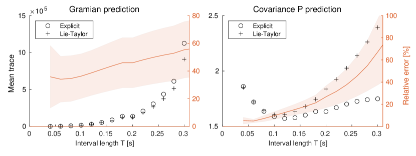
Figure 2: Numerical comparison between empirical and Lie-Taylor implementations for a single interval-filter update over varying interval lengths $T=K\Delta t$. The left plot shows results for the information Gramian $[\tens{\Lambda}^{\mathcal{Z}}(T)]_{\vec{e}_{0},\vec{e}_{0}}$ (the sub-block of the information matrix pertaining to initial ego-state $\vec{e}_{0}$), and the right plot does the same for the posterior covariance $\tens{P}(T)$ given $\tens{P}(0)=0.3\tens{I}$. Unsurprisingly, both the explicit and Lie-Taylor forms of $\tens{\Lambda}^{\mathcal{Z}}$ increase monotonically with $T$, as more measurements are included in the update. More interestingly, the relative error between ${\tens{\Lambda}^{\mathcal{Z}}}_{\text{exp}}$ and ${\tens{\Lambda}^{\mathcal{Z}}}_{\text{lie}}$ is near-constant over the horizon $T$. Moving to the covariance results in the right plot, note that the traces of the estimates track well for low $T$, but ultimately diverge exponentially as should be expected. Nevertheless, Lie-Taylor prediction of $\tens{P}(T)$ achieves reasonable accuracy over moderate intervals.

To evaluate the Lie-Taylor approximation described in Section 4, we can compare the approximation (25) with the explicit form (14). The results over varying interval length $T$ are plotted in Fig. 2, and show that while error of course grows with time, satisfactory approximation is achieved for time horizons corresponding to the accumulation of 10 or more measurements in either case. The computational advantage of our approximation is demonstrated in Table 1, in which computation times of the full $J_{\text{obs}}$ objective are compared.

6.2 Value of Posterior-Covariance Objective

We compared the performance of the posterior-covariance objective (6) to several heuristics:

• Maximizing landmark visibility: The method labeled max-visibility explicitly maximizes the total visibility along the trajectory, using the smooth visibility function given in (34)

  $$J_{\text{obs}}\triangleq\sum_{{\bar{k}}=1}^{{\bar{K}}}\sum_{n=1}^{N}\sigma\big{(}x(t_{k});\ell_{n}\big{)}.$$ (32)

• Max Fisher information: Following [20], max-gramian maximizes the smallest eigenvalue of the information Gramian (i.e., the Fisher information)

  $$J_{\text{obs}}\triangleq s_{1}\bigg{(}\sum_{{\bar{k}}=1}^{{\bar{K}}}\tens{Y}_{\vec{v}}[\tens{\Lambda}_{k}(x_{k},u_{k})]_{\vec{e}_{\bar{k}},\vec{e}_{\bar{k}}}\tens{Y}_{\vec{v}}^{\top}\bigg{)}.$$ (33)

  Because our sensor model (31) assumes unknown landmarks, absolute position is unobservable and therefore the position sub-matrix of $\tens{\Lambda}_{k}$ is always zero. Therefore we chose $\tens{Y}_{\vec{v}}$ to extract the velocity ${}^{w\!}\tilde{\vec{v}}$ sub-block of $\tens{\Lambda}_{k}$.

Additionally, we consider the efficacy of various approximations of the posterior-covariance during planning. For example, pc-exact uses the explicit form of the SIIF update (14), more accurately reflecting how estimator covariance is evaluated in practice. The method labeled pc-lie applies our Lie-Taylor approximation as given in (25) to computing $J_{\text{obs}}$, and pc-lie-cond takes the further approximation of assuming landmarks are fully known (that is, conditioning on rather than marginalizing out the landmark uncertainty).

These three posterior covariance methods, alongside the heuristics, were evaluated across a batch of 50 programmatically-generated motion-planning problems. In each trial, a random starting state and goal position is selected, and a corresponding baseline trajectory identified by minimizing $J_{c}$. Then this trajectory is refined under the augmented objective (4) via IPOPT [26], by replacing $J_{c}$ with $J_{\text{obs}}$ in the objective and constraining that the conventional cost $J_{c}$ may not increase beyond a fixed percentage ${r_{0}}$. As the tradeoff allowance ${r_{0}}$ is increased, the refined trajectory accepts larger increases in conventional cost $J_{c}$ for more significant reductions in the uncertainty objective $J_{\text{obs}}$. It is worth noting that while smooth FoV approximations (see App. A) may be used during optimization, the output trajectories are evaluated using the explicit measurement rollout (14) and hard visibility indicator $\mathbb{1}_{\text{vis}}(x;\ell)$. For our purposes here, pc-exact can be considered to define the Pareto front between observability and expedience.

Table 1: Averaged timing for SIIF covariance propagation on a consumer laptop over the full trajectory with $K=7$ and ${\bar{K}}=11$ (includes computation of analytic gradients required for optimization). As can be seen, our Lie-Taylor approximation represents a significant computational speedup, and exploitation of affine sensor models as in Alg. 2 allows for scaling to large numbers of landmarks.

Sensor	Bundling	$N=10$	$N=20$	$N=50$	$N=100$
Ortho cam	Explicit	265 [ms]	430 [ms]	966 [ms]	1862 [ms]
	Lie-Taylor	19 [ms]	33 [ms]	77 [ms]	151 [ms]
Ortho cam (affine)	Explicit	395 [ms]	406 [ms]	402 [ms]	420 [ms]
	Lie-Taylor	18 [ms]	17 [ms]	18 [ms]	17 [ms]

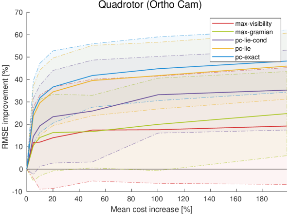
Figure 3: Each choice of $J_{\text{obs}}$ defines an effective trade-off curve between trajectory cost $J_{c}$ and estimation improvement (larger is better). We plot this curve by sweeping through the weighting parameter ${r_{0}}$ and aggregating results for a batch of random trials. Refinement based on heuristic objectives (see max-viz and max-gramian) or approximate sensor models (see pc-lie-cond) does not always yield significant estimation improvement. In contrast, minimization of the posterior covariance (via pc-lie or pc-exact) produces better estimation improvement for the same $J_{c}$ cost increase.

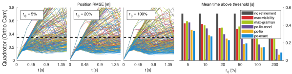
Figure 4: Evolution of the covariance traces shown for each refined trajectory, under varying settings of ${r_{0}}$. For a chosen “safety” threshold (dashed horizontal line), histograms of expected violation time are shown on the right. Without any refinement (black), uncertainty can grow without bound, but refinement under posterior-covariance objectives tend to keep uncertainty bounded, even for relatively low ${r_{0}}$. Other methods are significantly less effective at curbing uncertainty growth and ensuring safety.

Fig. 3 shows that our approximation pc-lie is nearly as effective as pc-exact in guiding the solver towards well-observable trajectories, achieving significant RMSE reductions at moderate marginal cost. Moreover, the heuristic objectives (max-viz and max-gramian) and incorrect sensor model (pc-lie-cond) are far less effective, often pushing the solver towards irrelevant and unhelpful solutions.

A central goal of observability-based planning is to avoid instances where uncertainty grows to dangerous or catastrophic levels. Fig. 4 plots position uncertainties along a large number of simulated trajectories for the two systems. Unrefined trajectories can develop large uncertainty, often well beyond safe levels, and heuristic refinement methods do not ensure good performance in all instances (even if they do well on average). In contrast, refinement via the pc-lie objective effectively moderates uncertainty growth across a variety of conditions, ensuring safety.

Note that our computational complexity results in Table 1 demonstrate that pc-lie is indeed far less expensive than pc-exact, while being nearly as effective in guiding the optimizer towards well-observable trajectories. This further validates our Lie-Taylor approximation and demonstrates its applicability for online trajectory generation.

7 Conclusions

Our results indicate that significant estimation improvement can be achieved by explicitly considering observability during trajectory generation. While posterior-covariance minimization is not novel in itself, we address several computational challenges that arise in the case of landmark-based estimators (i.e., visual SLAM). In doing so, we reduce algorithmic complexity from quadratic to near constant in the number of landmarks $N$, opening the door to online, real-time observability-aware planning. Furthermore, we identify a natural mechanism allowing for generic (and non-finite) landmark distributions, which ultimately enables extension of estimator performance prediction into unknown space.

In ongoing work, we are developing a real-time implementation capable of online motion planning for a VIO-enabled quadrotor. Furthermore, we hope to further explore the idea of learned landmark distributions.

Additionally, it is likely that orthographic projection will not ultimately provide an optimal analog for real-world cameras, which are usually modeled under perspective projection. Identifying a more accurate affine approximation of perspective projection is of direct interest, but for now is left as the subject of future work.

8 Acknowledgment

This work was supported by the Education Office at the Charles Stark Draper Laboratory, Inc. and by ARL DCIST under Cooperative Agreement Number W911NF-17-2-0181.

Appendix A Modeling Field-of-View

Because landmarks are often distributed non-uniformly, it is important that generated trajectories point sensors towards informative regions of the environment. For the purposes of continuous observability-aware optimization, we (similar to [28, 18]) seek a function $\sigma(x;\ell)\in[0,1]$ that smoothly interpolates the “hard” visibility indicator $\mathbb{1}_{\text{vis}}(x;\ell)\in\{0,1\}$.

As observed in Alg. 1 and 2, for our purposes we actually use the squared visibility $\sigma^{2}(x;\ell)$. One choice well-suited for a pinhole camera model is

$$\sigma^{2}(x,\ell)=\begin{cases}\frac{1}{2}\big{(}\cos a\theta+1\big{)}&|\theta|<\theta_{\text{max}}\\ 0&\text{else}\end{cases}$$ (34)

where

$$\theta=\cos^{-1}\left(\frac{\hat{\vec{e}}^{\top}{}^{c}\vec{l}}{{}^{c}\vec{l}^{\top}{}^{c}\vec{l}}\right)\qquad\in[0,\pi]$$ (35)

is the angle between the optical axis $\hat{\vec{e}}$ and the landmark vector ${}^{c}\vec{l}$ in the camera frame. The scaling parameter can be chosen $a=\pi/\theta_{\text{max}}$, ensuring that $\sigma^{2}$ is continuous and differentiable. In practice $\theta_{\text{max}}$ can be chosen to exactly match the (assumed conical) FoV of the sensor, or taken slightly larger to improve convergence of the optimization.

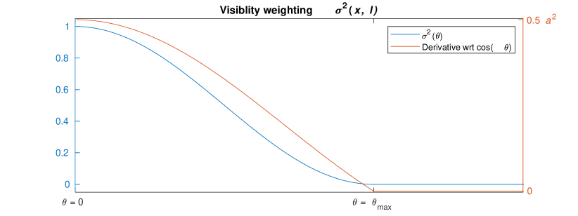
Figure 5: Our visibility weighting function (34) plotted against $\theta$ [blue]. The derivative $\frac{\partial\sigma^{2}(\cos\theta)}{\partial\cos\theta}$ is plotted as a function of $\theta$ in red, and both are clearly continuous (and bounded) over the entire domain $[0,\pi]$.

It may appear problematic that the inverse cosine $\cos^{-1}(y)$ is not differentiable in its argument at $y=\cos\theta=1\iff\theta=0$ (and its derivative in the open interval $\theta\in(0,\pi]$ is unbounded). Fortunately, the composite function $\sigma^{2}(y)$ is differentiable in $y$ for all $\theta\in[0,\pi]$ with bounded derivative, as shown in Fig. 5.

Appendix B Computing Gradients through Marginalization

As pointed out by Mourikis et al.[17], computing a left-nullspace matrix ${\mathcal{Q}^{({n})}}$ of $\mathcal{L}^{({n})}$ satisfying (13) can be accomplished via a partial SVD.

$$\mathcal{L}^{({n})}=\tens{U}\begin{bmatrix}\tens{\Sigma}_{1}\\ \tens{0}_{r\times n}\end{bmatrix}\tens{V}^{\top}\quad\implies\quad{\mathcal{Q}^{({n})}}=\tens{U}\begin{bmatrix}\tens{0}_{n\times r}\\ \tens{I}_{r}\end{bmatrix}$$ (36)

Then the linearized residual (12) can be made independent of landmark error $\vec{\tilde{l}}^{({n})}$ by application of ${\mathcal{Q}^{({n})}}^{\top}$. However, in a continuous optimization framework, we need to be able to compute gradients through this marginalization process.

While the SVD is differentiable in general [23], we identify a simpler form of $\mathop{}\!\mathrm{d}{\mathcal{Q}^{({n})}}$. Letting $\mathcal{L}^{({n})}$ have dimension $m\times n$ with $m>n$, then ${\mathcal{Q}^{({n})}}$ will have dimension $m\times(m-n)$. Letting $r=m-n$, then a suitable $\mathop{}\!\mathrm{d}{\mathcal{Q}^{({n})}}$ must also be $m\times r$ and satisfy differentiated forms of the constraints (13).

$$\mathop{}\!\mathrm{d}{\mathcal{Q}^{({n})}}^{\top}\mathcal{L}^{({n})}+{\mathcal{Q}^{({n})}}^{\top}\mathop{}\!\mathrm{d}\mathcal{L}^{({n})} =\tens{0}_{r\times n}$$ (37)

$$\mathop{}\!\mathrm{d}{\mathcal{Q}^{({n})}}^{\top}{\mathcal{Q}^{({n})}}+{\mathcal{Q}^{({n})}}^{\top}\mathop{}\!\mathrm{d}{\mathcal{Q}^{({n})}} =\tens{0}_{r\times r}$$ (38)

It is straightforward to verify that these conditions will be satisfied by any $\mathop{}\!\mathrm{d}{\mathcal{Q}^{({n})}}$ such that

$$\mathop{}\!\mathrm{d}{\mathcal{Q}^{({n})}} =\tens{U}\begin{bmatrix}\tens{Z}_{1}\\ \tens{Z}_{2}\end{bmatrix}$$ (39)

$$\tens{Z}_{1} =-\tens{\Sigma}_{1}^{-1}\tens{V}^{\top}\mathop{}\!\mathrm{d}\tens{H}_{\ell}^{\top}{\mathcal{Q}^{({n})}}$$ (40)

$$\tens{Z}_{2} =-\tens{Z}_{2}^{\top}\quad\text{(skew-symmetric)}$$ (41)

where the inverse of diagonal $\tens{\Sigma}_{1}$ is trivial to compute, and $\tens{Z}_{2}$ can conveniently be taken as $\tens{0}_{n\times n}$. In practice, this recipe is inexpensive to compute and straightforward to implement.

References

- [1] Arneberg, J., Tal, E., Karaman, S.: Guidance laws for partially-observable interception based on linear covariance analysis. In: Proc. IEEE Conf. Int. Rob. Sys. (IROS), pp. 4185–4191. IEEE (2018)
- [2] Bloesch, M., Burri, M., Omari, S., Hutter, M., Siegwart, R.: Iterated extended kalman filter based visual-inertial odometry using direct photometric feedback. The International Journal of Robotics Research 36(10), 1053–1072 (2017)
- [3] Bry, A., Roy, N.: Rapidly-exploring random belief trees for motion planning under uncertainty. In: Proc. IEEE Conf. Robot. Autom. (ICRA), pp. 723–730. IEEE (2011)
- [4] Burri, M., Nikolic, J., Gohl, P., Schneider, T., Rehder, J., Omari, S., Achtelik, M.W., Siegwart, R.: The euroc micro aerial vehicle datasets. Int. J. of Robotics Research (2016). 10.1177/0278364915620033. URL http://ijr.sagepub.com/content/early/2016/01/21/0278364915620033.abstract
- [5] Conticelli, F., Bicchi, A., Balestrino, A.: Observability and nonlinear observers for mobile robot localization. IFAC Proceedings Volumes 33(27), 663–668 (2000)
- [6] Davison, A.J., Reid, I.D., Molton, N.D., Stasse, O.: Monoslam: Real-time single camera slam. IEEE transactions on pattern analysis and machine intelligence 29(6), 1052–1067 (2007)
- [7] Dellaert, F., Kaess, M.: Square root sam: Simultaneous localization and mapping via square root information smoothing. Int. J. of Robotics Research 25(12), 1181–1203 (2006)
- [8] Elimelech, K., Indelman, V.: Scalable sparsification for efficient decision making under uncertainty in high dimensional state spaces. In: Proc. IEEE Conf. Int. Rob. Sys. (IROS), pp. 5668–5673. IEEE (2017)
- [9] Elisha, Y.B., Indelman, V.: Active online visual-inertial navigation and sensor calibration via belief space planning and factor graph based incremental smoothing. In: Proc. IEEE Conf. Int. Rob. Sys. (IROS), pp. 2616–2622. IEEE (2017)
- [10] Falanga, D., Foehn, P., Lu, P., Scaramuzza, D.: PAMPC: Perception-aware MPC for quadrotors. In: Proc. IEEE Conf. Int. Rob. Sys. (IROS), pp. 1–8. IEEE (2018)
- [11] Indelman, V., Carlone, L., Dellaert, F.: Planning in the continuous domain: A generalized belief space approach for autonomous navigation in unknown environments. Int. J. of Robotics Research 34(7), 849–882 (2015)
- [12] Kaess, M., Johannsson, H., Roberts, R., Ila, V., Leonard, J.J., Dellaert, F.: isam2: Incremental smoothing and mapping using the bayes tree. Int. J. of Robotics Research p. 0278364911430419 (2011)
- [13] Kanade, T., Morris, D.D.: Factorization methods for structure from motion. Philosophical Transactions of the Royal Society of London 356(1740), 1153–1173 (1998)
- [14] Kopitkov, D., Indelman, V.: No belief propagation required: Belief space planning in high-dimensional state spaces via factor graphs, the matrix determinant lemma, and re-use of calculation. Int. J. of Robotics Research 36(10), 1088–1130 (2017)
- [15] Krener, A.J., Ide, K.: Measures of unobservability. In: Conf. on Dec. and Control (CDC), pp. 6401–6406. IEEE (2009)
- [16] Mariottini, G.L., Morbidi, F., Prattichizzo, D., Vander Valk, N., Michael, N., Pappas, G., Daniilidis, K.: Vision-based localization for leader–follower formation control. IEEE Trans. Robotcs 25(6), 1431–1438 (2009)
- [17] Mourikis, A.I., Roumeliotis, S.I.: A multi-state constraint kalman filter for vision-aided inertial navigation. In: Proc. IEEE Conf. Robot. Autom. (ICRA), pp. 3565–3572. IEEE (2007)
- [18] Murali, V., Spasojevic, I., Guerra, W., Karaman, S.: Perception-aware trajectory generation for aggressive quadrotor flight using differential flatness. In: American Control Conference (ACC) (2019)
- [19] Nobre, F., Heckman, C.: Learning to calibrate: Reinforcement learning for guided calibration of visual–inertial rigs. Int. J. of Robotics Research (2019)
- [20] Preiss, J.A., Hausman, K., Sukhatme, G.S., Weiss, S.: Simultaneous self-calibration and navigation using trajectory optimization. Int. J. of Robotics Research (2018)
- [21] Prentice, S., Roy, N.: The belief roadmap: Efficient planning in belief space by factoring the covariance. Int. J. of Robotics Research 28(11-12), 1448–1465 (2009)
- [22] Rafieisakhaei, M., Chakravorty, S., Kumar, P.: The use of the observability gramian for partially observed path planning problems. In: Conf. on Dec. and Control (CDC), pp. 1523–1528. IEEE (2017)
- [23] Townsend, J.: Differentiating the singular value decomposition. https://j-towns.github.io/papers/svd-derivative.pdf (2016). Accessed: 2019-05-14
- [24] Van Den Berg, J., Abbeel, P., Goldberg, K.: LQG-MP: Optimized path planning for robots with motion uncertainty and imperfect state information. Int. J. of Robotics Research 30(7), 895–913 (2011)
- [25] Van Den Berg, J., Patil, S., Alterovitz, R.: Motion planning under uncertainty using iterative local optimization in belief space. Int. J. of Robotics Research 31(11), 1263–1278 (2012)
- [26] Wächter, A., Biegler, L.T.: On the implementation of an interior-point filter line-search algorithm for large-scale nonlinear programming. Mathematical programming 106(1), 25–57 (2006)
- [27] Zhang, Z., Scaramuzza, D.: Perception-aware receding horizon navigation for MAVs. In: Proc. IEEE Conf. Robot. Autom. (ICRA), pp. 2534–2541. IEEE (2018)
- [28] Zhang, Z., Scaramuzza, D.: Beyond point clouds: Fisher information field for active visual localization. In: Proc. IEEE Conf. Robot. Autom. (ICRA). IEEE (2019)