Steady waves in flows over periodic bottoms

Abstract

We study the formation of steady waves in two-dimensional fluids under a current with mean velocity $c$ flowing over a periodic bottom. Using a formulation based on the Dirichlet-Neumann operator, we establish the unique continuation of a steady solution from the trivial solution when a flat bottom is perturbed, except for a sequence of velocities $c_{k}$. The main contribution is the proof that at least two steady solutions exist close to a non-degenerate $S^{1}$-orbit of non-constant steady waves when a flat bottom is perturbed. Consequently, we obtain persistence of at least two steady waves close to a non-degenerate $S^{1}$-orbit of Stokes waves bifurcating from the velocities $c_{k}$.

1 Introduction

Stokes’ analysis of periodic water waves in a region of infinite depth heralded much interest in the field of fluid dynamics. In the early twentieth century, Nekrasov and Levi-Civita first rigorously proved the existence of the Stokes waves (two-dimensional $2\pi$-periodic gravity waves on water of infinite depth). Stokes waves are steady solutions when they are viewed in a reference frame moving with speed $c$. This result was extended to the case of finite flat bottoms by Struik. These waves appear as a bifurcation from the trivial solution for the velocities

$$c_{k}:=\left(g\frac{1}{\left|k\right|}\tanh(h\left|k\right|)\right)^{1/2},\qquad k\in\mathbb{N},$$

where $g$ is the acceleration of gravity and $h$ is the deepness of the bottom. Stokes conjectured that the primary branch from $c_{1}$ is limited by an extreme wave with a singularity at their crest forming a $2\pi/3$-angle. The first rigorous global bifurcation of traveling waves (Stokes waves) was presented in [17], but Stokes conjecture was proved only recently in [2] and [22].

For varying bottoms, the Euler equation is not invariant by translations anymore, i.e., the problem cannot be reduced to a steady wave in a moving reference frame. On the other hand, for $2\pi$-periodic bottoms $-h+b(x)$, steady waves exist in a stream current of mean velocity $c$ in a fixed reference frame. The formation of steady waves in two-dimensional flows for near-flat bottoms (with small $b$) has been studied previously in [12], [16], [20] and [23]. The first rigorous result in [12] proves the existence of one steady solution for bottoms with two extrema per period, except for the sequence of degenerate values $c_{k}$. Those results were extended in [16] to any near-flat bottom and to general bottoms in the case that $c$ is large enough. Under similar hypothesis, according to [20], the top of the fluid follows the bottom when $c>c_{\ast}$, but it inverts when $c<c_{\ast}$. Later on, the existence of steady solutions for a three-dimensional fluid was analyzed in [23].

The purpose of this work is to investigate further the existence of two-dimensional steady waves over a periodic bottom. We formulate the Euler equation as a Hamiltonian system similarly to [25]. The work [19] contains a short exposition of the different formulations of the Euler equation. We formulate the Hamiltonian using the Dirichlet-Neumann operator and a mean stream current with velocity $c$ analogously to the formulations in [6], [7] and [9]. Using this approach, in Theorem 10 we recover the result in [16] regarding the unique continuation of the trivial solution for small perturbations of bottom $b$, except for the sequence of velocities $c_{k}$.

The Hamiltonian for water waves in flat bottoms $b=0$ is $S^{1}$-invariant, where the group

$$S^{1}:=\mathbb{R}/2\pi\mathbb{Z}$$

acts by translations in the periodic domain $[0,2\pi]$. The $S^{1}$-invariance of the Hamiltonian implies that its Hessian at the trivial solution with velocity $c_{k}$ has a two-dimensional kernel. The paper [13] presents an analysis of the set of solutions near the bifurcation point $c=c_{k}$ by classifying the patterns of bifurcation according to the shape of the bottom, but only in the space of even surfaces and for even bottoms, which simplifies the problem because the kernel becomes one dimensional under these constraints. The analysis of the bifurcation diagram for general surfaces and small bottoms near $c=c_{k}$ is difficult because the kernel is two-dimensional, but the Hamiltonian is not $S^{1}$-invariant anymore. Indeed, even to determine the splitting of linear eigenvalues of the Hessian near the degenerate velocities $c_{k}$ is a challenging task; for example, this phenomenon is analyzed in [5]. On the other hand, our Hamiltonian formulation allows us to prove the persistence of solutions far from the degenerate velocities. Specifically,

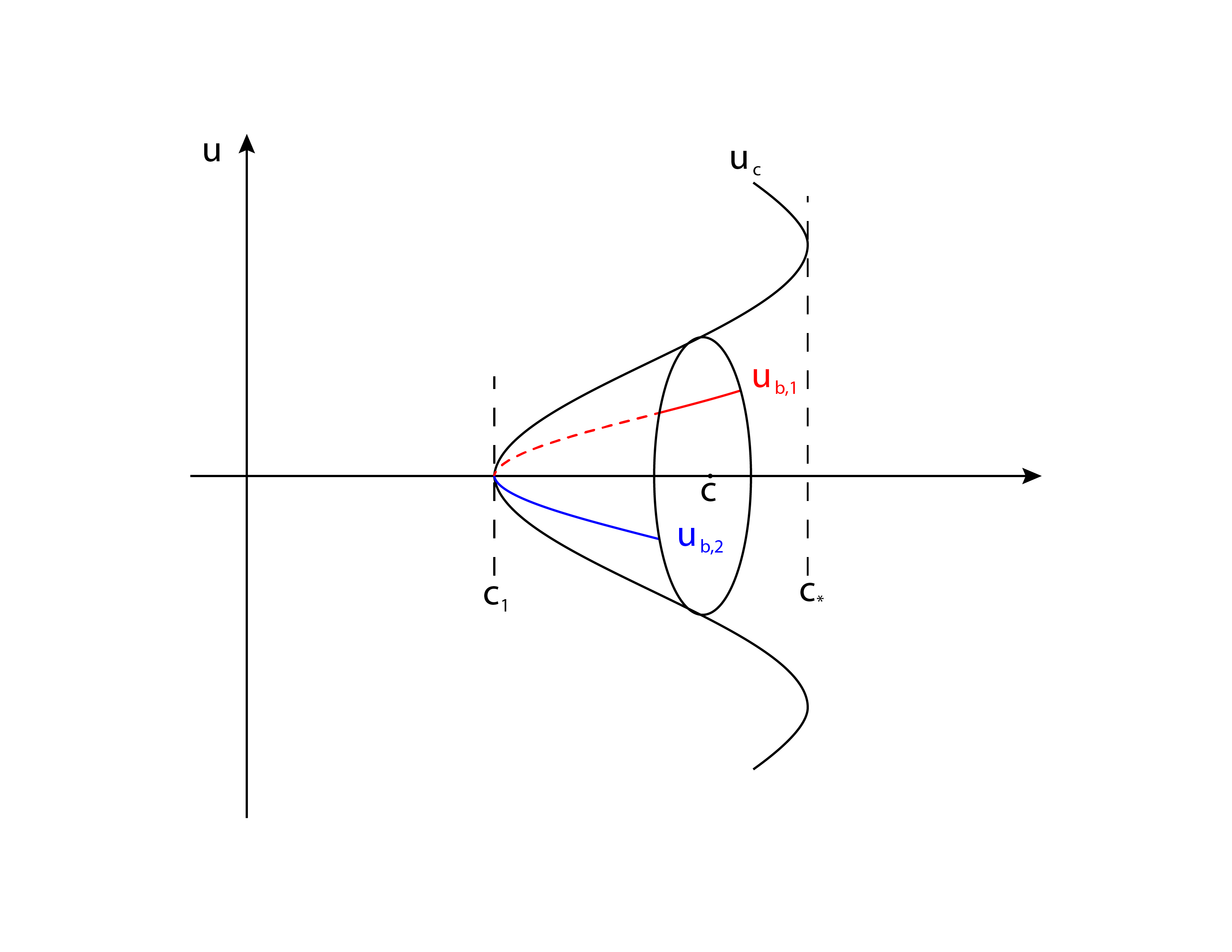
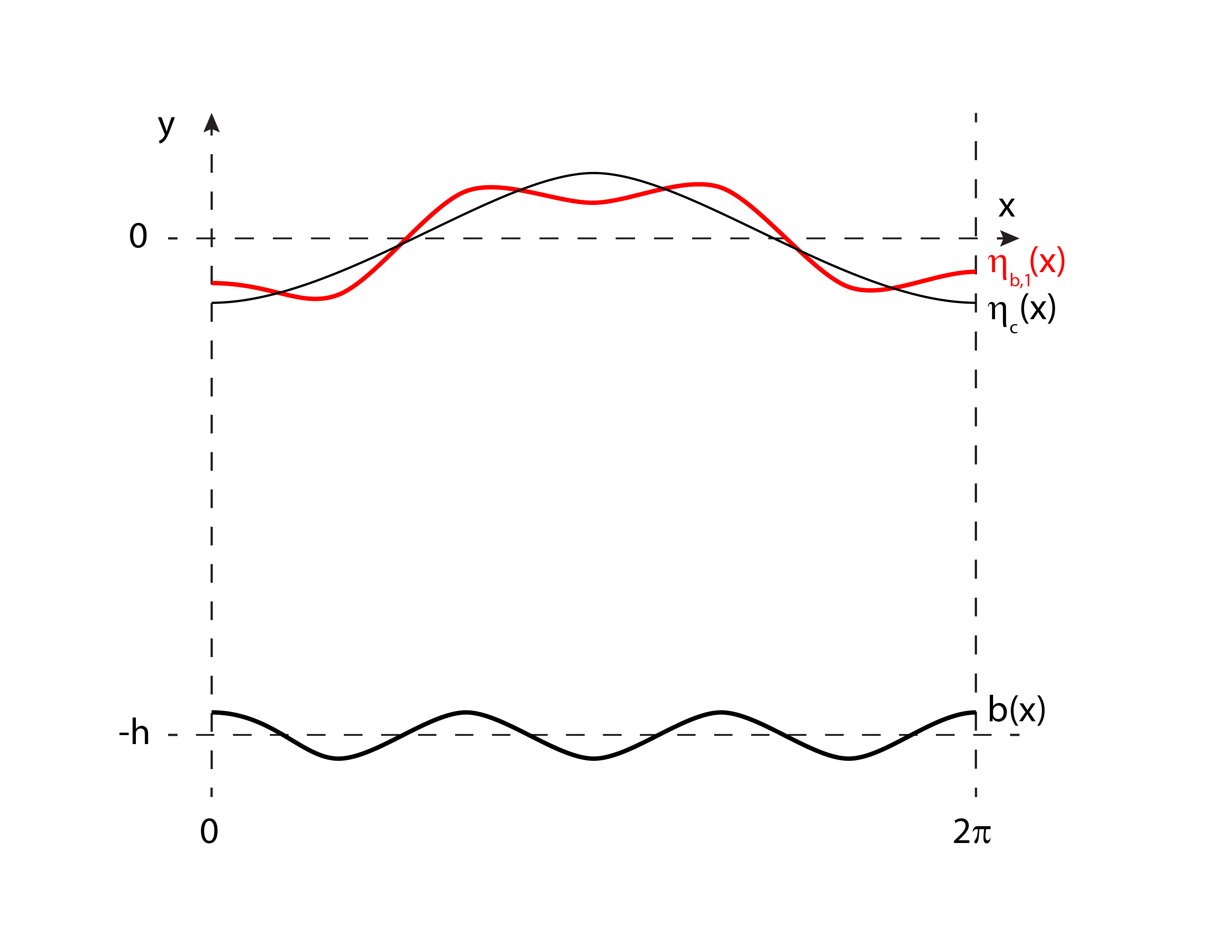
Figure 1: Left: Bifurcation diagram of the family of $S^{1}$-orbits of solutions $u_{c}$ (Stokes wave). At least two solutions $u_{b,1}$ (red) and $u_{b,2}$ (blue) persist when $b$ is small, except for degenerate values such as $c_{1}$ and $c_{\ast}$. Right: Illustration of the surface $\eta_{b,1}(x)$ (red)  near the surface $\eta_{c}(x)$ (Stokes wave).

Main Result. In Theorem 12 we prove that at least two steady waves exist close to the non-degenerate $S^{1}$-orbit (Definition 11) of a non-constant steady wave when a flat bottom is perturbed. Consequently, this theorem implies the persistence of at least two steady waves close to the primary branch of Stokes waves which are non-degenerate. This phenomenon is illustrated in Figure 1.

We will briefly discuss the non-degeneracy property of an $S^{1}$-orbit of the primary branch of Stokes waves. The appearance of a degenerate $S^{1}$-orbit in a branch of Stokes waves leads generically to the existence of bifurcation (Figure 1). For a fluid with infinite depth, the article [3] proves that the Morse index of solutions along the primary branch of Stokes waves bifurcating from $c_{1}$ diverges as the branch approaches the extremal wave (conjectured by Stokes). These analytic methods imply that the branch of Stokes waves, parameterized by $\lambda$, has a countable number of critical values $\left(\lambda_{j}\right)_{j\in\mathbb{N}}$ containing turning points (fold bifurcations) or harmonic bifurcations. The numerical evidence is that only turning points occur. Therefore, the results in [3] imply that the primary branch of Stokes waves is non-degenerate (in the subspace of even periodic functions) except for set of critical values $\left(\lambda_{j}\right)_{j\in\mathbb{N}}$.

To the best of our knowledge, the bifurcation from the branch of Stokes waves has not been established rigorously for a fluid with a flat bottom ($b=0$). The numerical computations in [8] indicate that only a countable set of turning points occur in the primary branch of Stokes waves arising from $c_{1}$. Given this numerical evidence, we conjecture that the $S^{1}$-orbits of the primary branch of Stokes waves, parameterized by $\lambda$, is non-degenerate except for a countable set of critical values $\left(\lambda_{j}\right)_{j\in\mathbb{N}}$. If this conjecture is true, our theorem proves the persistence of at least two steady waves close to the primary branch of Stokes waves, except for the hypothetical set of critical values $\left(\lambda_{j}\right)_{j\in\mathbb{N}}$.

A possible approach to prove this conjecture is to extend the methods in [3] to the Babenko formulation for a fluid with a flat bottom in [18]. But this challenging task is beyond the scope of our presentation. Our main contribution is to present a novel mathematical framework to prove the persistence of steady waves different to the ones studied previously from a flat surface. These steady waves can be found close to the Stokes waves or even its secondary bifurcations. These steady waves have been observed and described in the formation of dunes (out of phase waves) and in antidunes (in phase waves).

Theorem 12 is proved by applying a Lyapunov-Schmidt reduction in a Sobolev space of $2\pi$-periodic function to solve the normal components to a non-degenerate $S^{1}$-orbit. The result is obtained from the fact that the reduced Hamiltonian (defined in the domain $S^{1}$) has at least two critical points. The Hamiltonian formulation presented in this work can be used to study other problems of interest such as the existence of steady waves in more dimensions. However, for torus domains $\mathbb{T}^{n}$ it is necessary to consider surface tension to avoid the small divisor problem, see [7] for references. In such a case, one can apply Lusternik-Schnirelmann category to prove the persistence of at least $n+1$ solutions from a non-degenerate $\mathbb{T}^{n}$-orbit of steady waves (Stokes waves). Lusternik-Schnirelmann category has been used to prove the persistence of solutions in finite-dimensional Hamiltonian systems in [11].

The paper is organized as follows. In Section 2, we define the Hamiltonian using the Dirichlet-Neumann operator. In Section 3, we prove the continuation of the trivial solution for small $b$. In Section 4, we prove the persistence of at least two steady waves near a non-degenerate $S^{1}$-orbit of steady waves for small $b$.

2 Formulation for two-dimensional steady water waves

We study the problem of steady waves in the periodic domain $S^{1}=\mathbb{R}/2\pi\mathbb{Z}$. In this domain, we define the Sobolev space of $2\pi$-periodic functions,

$$H^{s}\left(S^{1};\mathbb{R}\right)=\left\{u(x)=\sum_{k\in\mathbb{Z}}u_{k}e^{ixk}\in L^{2}:\left|u\right|_{s}^{2}=\sum_{k\in\mathbb{Z}}\left(1+k^{2}\right)^{s}\left|u_{k}\right|^{2}<\infty\right\},\qquad s\geq 0\text{.}$$

The free surface of the fluid is represented by the curve $y=\eta(x)$, and the bottom of the fluid by $y=-h+b(x)$, where $b$ is a $2\pi$-periodic variation from the mean deep $-h$.

In the domain

$$D_{b,\eta}=\left\{\left(x,y\right)\in S^{1}\times\mathbb{R}:-h+b(x)<y<\eta(x)\right\}\text{,}$$ (1)

the Hamiltonian for the time-dependent Euler equation is given by $H=K+E$, where the kinetic and potential energy are

$$K=\int_{S^{1}}\left(\int_{-h+b}^{\eta}\frac{1}{2}\left|\nabla\phi\right|^{2}dy\right)dx,\qquad E=\int_{S^{1}}\frac{1}{2}g\eta^{2}~{}dx\text{.}$$

According to [24], the requirement that the functional $H$ is stationary with respect to independent variations $\delta\eta$ and $\delta\phi$ gives the set of equations

$$\Delta\phi = 0\text{ in }D_{b,\eta}\text{,}$$

$$\frac{\partial\phi}{\partial n} = n\cdot\nabla\phi=0\text{ in }\partial D_{b,\eta}\text{,}$$

and the kinematic boundary condition and Bernoulli condition at $y=\eta(x)$,

$$\partial_{t}\eta = \partial_{y}\phi-\partial_{x}\eta\cdot\partial_{x}\phi,$$

$$\partial_{t}\phi = -\frac{1}{2}\left|\nabla\phi\right|^{2}-g\eta,$$

see also [4] for details.

The Zakharov formulation assigns a Hamiltonian structure to the dynamics of waves. Zakharov discovered in [25] that a subtle aspect is the choice of the canonical variables $\xi(x,t)=\phi(x,\eta(x,t),t)$ and $\eta(x,t)$ for the phase space of the time-dependent Euler equation satisfying the kinematic boundary condition $\partial_{t}\eta=\delta_{\xi}H$ and the Bernoulli condition $\partial_{t}\xi=-\delta_{\eta}H$. In particular, the steady waves are critical points of the Hamiltonian $H(\eta,\xi)$ in the domain $D_{b,\eta}$.

Furthermore, if we look for critical points of $H(\eta,\xi)$ restricted by the constraint of zero excess of mass

$$m(\eta):=\int_{S^{1}}\eta(x)=0\in\mathbb{R}\text{,}$$

then these critical points satisfy instead the equations $\delta_{\xi}H=0$ and $\delta_{\eta}H+\lambda\delta_{\eta}m(\eta)=0$, where $\lambda$ is the Lagrange multiplier. Since $\delta_{\eta}m(\eta)=1$, the second equation is up to a constant the Bernoulli condition

$$\delta_{\eta}H+\lambda=\frac{1}{2}\left|\nabla\phi\right|^{2}+g\eta+\lambda=0.$$

Hereafter, we study the problem of steady waves as critical points of the Hamiltonian $H(\eta,\xi)$ restricted to the space of functions with zero excess of mass $\eta\in H_{0}^{s+1}$, where

$$H_{0}^{s}=\left\{\eta\in H^{s}:\int_{S^{1}}\eta(x)~{}dx=0\right\},\qquad s\geq 0.$$

2.1 Dirichlet-Neumann operator

To obtain an expression for the Hamiltonian $H(\eta,\xi)$ we require the Dirichlet-Neumann operator. Hereafter the symbols $N_{\eta}\cdot\nabla$ and $N_{b}\cdot\nabla$ represent the external normal derivatives (not normalized) at the top and bottom of the domain $D_{b,\eta}$,

$$N_{\eta}\cdot\nabla=\partial_{y}-\partial_{x}\eta\partial_{x},\qquad N_{b}\cdot\nabla=-\partial_{y}+\partial_{x}b\partial_{x}~{}.$$

Definition 1

The Dirichlet-Neumann operator is defined by

$$G(\eta;b)\xi=\left.N_{\eta}\cdot\nabla\Phi\right|_{y=\eta(x)},$$

where $\Phi$ is the unique harmonic function in $D_{b,\eta}$ that satisfies the boundary condition $\xi(x)=\Phi(x,\eta(x))$ at the top $y=\eta(x)$ and $N_{b}\cdot\nabla\Phi=0$ at the bottom $y=-h+b(x)$.

By the continuous embedding $H^{s+1}\hookrightarrow C^{1}(S^{1};\mathbb{R})$ with $s>1/2$, there is a constant $\gamma$ such that $\left|\cdot\right|_{C^{1}}\leq\gamma\left|\cdot\right|_{H^{s+1}}$. Therefore $\left|b\right|_{C^{0}}\leq\gamma\varepsilon$ if $\left|b\right|_{s+1}\leq\varepsilon$. The condition $\left|b\right|_{s+1}\leq\varepsilon$ and $\eta\geq-h+2\gamma\varepsilon$ imply that the bottom $y=-h+b(x)$ and the top $y=\eta(x)$ remain at a $\gamma\varepsilon$-distance,

$$\left|\eta-\left(-h+b\right)\right|_{C^{0}}\geq\left|h+\eta\right|_{C^{0}}-\left|b\right|_{C^{0}}\geq\gamma\varepsilon\text{.}$$ (2)

Proposition 2

By Theorem A.11 in [19], the Dirichlet-Neumann operator

$$G(\eta;b):H^{s+1}\rightarrow H^{s},\qquad s>1/2,$$

is analytic as a function of $(\eta;b)\in H_{0}^{s+1}\times H^{s+1}$ if $\left|b\right|_{s+1}\leq\varepsilon$ with $s>1/2$ and $\eta(x)>-h+2\gamma\varepsilon$ for $x\in S^{1}$.

2.2 The current of mean velocity $c$

We define the cylinder-like domain

$$D_{b}=\left\{\left(x,y\right)\in S^{1}\times\mathbb{R}:-h+b(x)<y\right\}.$$ (3)

Notation $b\lesssim a$ means that there is a positive constant $C$ such that $b\leq Ca$ for all $a>0$ sufficiently small.

In section 2.4 we prove the following estimate for the harmonic function $\Phi_{b}$.

Theorem 3

There is an $\varepsilon>0$ such that if $\left|b\right|_{s+1}\leq\varepsilon$ with $s>1/2$, then there is a unique harmonic function $\Phi_{b}\left(x,y\right):D_{b}\rightarrow\mathbb{R}$ with boundary conditions

$$\lim_{y\rightarrow\infty}\nabla\Phi_{b}(x,y)=0,\qquad\lim_{y\rightarrow\infty}\Phi_{b}(x,y)=0,$$ (4)

and

$$N_{b}\cdot\nabla\left(\Phi_{b}+x\right)=0~{},\qquad y=-h+b(x).$$ (5)

Furthermore, the function $\Phi_{b}\left(x,y\right)$ satisfies the estimate

$$\left|\Phi_{b}\right|_{C^{k}(\bar{D})}\lesssim\left|b\right|_{s+1}~{},\qquad k\in\mathbb{N}\text{,}$$ (6)

where $\bar{D}\subset D_{2\gamma\varepsilon}$ is a compact set.

If $b\in H^{s+1}$ with $s>1/2$, we define $\nabla\Psi_{c}=c(x+\Phi_{b})$ as the current of mean velocity $c$. The function $\Psi_{c}$ is the unique harmonic function in $D_{b}$ with boundary conditions

$$\lim_{y\rightarrow\infty}\nabla\Psi_{c}(x,y)=(c,0),\qquad\lim_{y\rightarrow\infty}\Psi_{c}(x,y)=cx,$$

and zero Neumann boundary condition at the bottom

$$N_{b}\cdot\nabla\Psi_{c}=0~{},\qquad y=-h+b.$$

Remark 4

Actually, the harmonic function $\Psi_{1}=x+\Phi_{b}$ generates the De Rham $1$-cohomology group $H^{1}(D_{b})=\mathbb{R}$ in the cylindrical domain $D_{b}$. Indeed, $H^{1}(D_{b})$ is generated by the form $\Omega=-\partial_{y}\Psi_{1}dx+\partial_{x}\Psi_{1}dy$ that is closed, $d\Omega=\Delta\Psi_{1}dx\wedge dy=0$, but not exact. The Hodge-Helmholtz decomposition [10] implies that any vector field $u$ defined in the domain $D_{b}$ with the boundary conditions $\lim_{y\rightarrow\infty}u=(c,0)$ and $N_{b}\cdot\nabla u=0$ at $y=-h+b(x)$ is decomposed into three components: a divergence-free (incompressible), a rotation-free (irrotational), and a harmonic (translational) component. The component $\nabla\Psi_{1}$ is harmonic in the sense that it is divergence-free $\nabla\cdot\nabla\Psi_{1}=\Delta\Psi_{1}=0$ and curl-free $\nabla^{\perp}\cdot\nabla\Psi_{1}=0$, where $\nabla^{\perp}=(-\partial_{y},\partial_{x})$. For more dimensions, the domain $D_{b}=\left\{\left(x,y\right)\in\mathbb{T}^{n}\times\mathbb{R}:-h+b(x)<y\right\}$ has $n$ translational fields $\nabla\Psi_{j}$ corresponding to the De Rham $1$-cohomology $H^{1}(D_{b})=\mathbb{R}^{n}$. Our analysis can be extended to torus domains of general dimension $\mathbb{T}^{n}$ by considering these $n$ fields $\nabla\Psi_{j}$ that represent the currents in the different directions of the domain $D_{b}$.

2.3 The gradient of the Hamiltonian

The kinetic energy for $\phi=\Phi+\Psi_{c}$ (where $\Phi$ is a perturbation of the current generated by $\Psi_{c}$) is given by

$$K=\int_{S^{1}}\int_{-h+b}^{\eta}\frac{1}{2}\left|\nabla\phi\right|^{2}dy~{}dx=\int_{S^{1}}\int_{-h+b}^{\eta}\frac{1}{2}\left|\nabla\Phi+\nabla\Psi_{c}\right|^{2}dy~{}dx.$$

We are ready to establish the formulation of the kinetic energy $K$ in terms of the variables $(\eta,\xi)\in H_{0}^{s+1}\times H^{s+1}$ and the parameters $b\in H^{s+1}$ and $c\in\mathbb{R}$.

Proposition 5

If $\eta$ has zero-average, then the kinetic energy in terms of the variables $\eta(x)$ and $\xi(x)=\Phi(x,\eta(x))$, where $\Phi$ is the harmonic function in Definition 1, is given by

$$K=\int_{S^{1}}\left(\frac{1}{2}\xi G(\eta;b)\xi+c\xi\left(N_{\eta}\cdot\nabla\Phi_{b}-\partial_{x}\eta\right)+\frac{c^{2}}{2}\eta+\frac{c^{2}}{2}\Phi_{b}\left(N_{\eta}\cdot\nabla\Phi_{b}-2\partial_{x}\eta\right)\right)dx+C,$$

where $\Phi_{b}$ and $N_{\eta}\cdot\nabla\Phi_{b}$ are functions evaluated at $y=\eta(x)$ and $C$ is a constant depending on $b\in H^{s+1}$ and $c\in\mathbb{R}$, but independent of $(\eta,\xi)$.

Proof. The kinetic energy is

$$K=\int_{D_{b,\eta}}\frac{1}{2}\nabla\Phi\cdot\nabla\left(\Phi+2\Psi_{c}\right)+\int_{D_{b,\eta}}\frac{1}{2}\left|\nabla\Psi_{c}\right|^{2}~{}.$$

Since $\Phi$ and $\Psi_{c}$ are harmonic functions, by the Divergence Theorem we have

$$K=\int_{\partial D_{b,\eta}}\frac{1}{2}\Phi\nabla\left(\Phi+2\Psi_{c}\right)\cdot N~{}dS+\int_{D_{b,\eta}}\frac{1}{2}\left|\nabla\Psi_{c}\right|^{2}\text{,}$$

where $N$ is the normal of $\partial D_{b,\eta}$. Since $\nabla\left(\Phi+2\Psi_{c}\right)$ is $2\pi$-periodic, then

$$K=\frac{1}{2}\int_{S^{1}}\left.\Phi N_{\eta}\cdot\nabla\left(\Phi+2\Psi_{c}\right)\right|_{y=\eta}+\left.\Phi N_{b}\cdot\nabla\left(\Phi+2\Psi_{c}\right)\right|_{y=-h+b}dx+\int_{D_{b,\eta}}\frac{1}{2}\left|\nabla\Psi_{c}\right|^{2}\text{.}$$

Given that $\Phi$ and $\Psi_{c}$ satisfy the Neumann boundary conditions at the bottom, while $N_{\eta}\cdot\nabla\Phi=G(\eta;b)\xi$ and $N_{\eta}\cdot\nabla\Psi_{c}=c(N_{\eta}\cdot\nabla\Phi_{b}-\partial_{x}\eta)$ at the top $y=\eta(x)$, the kinetic energy becomes

$$K=\int_{S^{1}}\frac{1}{2}\xi G(\eta;b)\xi+c\xi\left(\left(N_{\eta}\cdot\nabla\Phi_{b}\right)_{y=\eta}-\partial_{x}\eta\right)~{}dx+\int_{D_{b,\eta}}\frac{1}{2}\left|\nabla\Psi_{c}\right|^{2},$$

where

$$\int_{D_{b,\eta}}\frac{1}{2}\left|\nabla\Psi_{c}\right|^{2}=\int_{D_{b,\eta}}\frac{1}{2}c^{2}\left|\nabla(\Phi_{b}+x)\right|^{2}=\frac{c^{2}}{2}\int_{D_{b,\eta}}\left(\nabla\Phi_{b}\cdot\nabla\left(\Phi_{b}+2x\right)+1\right).$$

Since $\eta$ has zero average, then

$$\int_{D_{b,\eta}}1=\int_{S^{1}}(\eta(x)+h-b(x))~{}dx=2\pi\left(h-\int_{S^{1}}b\right).$$

Thus, by the Divergence Theorem, and the fact that $\nabla\left(\Phi_{b}+x\right)_{y=-h+b}=0$, we have

$$\int_{D_{b,\eta}}\frac{1}{2}\left|\nabla\Psi_{c}\right|^{2}=\frac{c^{2}}{2}\int_{S^{1}}\left(\eta(x)+\left(\Phi_{b}~{}N_{\eta}\cdot\nabla\left(\Phi_{b}+2x\right)\right)_{y=\eta}~{}+\left(\Phi_{b}~{}\partial_{x}b\right)_{y=-h+b}\right)dx+\pi hc^{2}.$$

The result follows with the constant

$$C:=\pi c^{2}\left(h-\int_{S^{1}}b\right)+\frac{c^{2}}{2}\int_{S^{1}}\partial_{x}b(x)\Phi_{b}(x,-h+b(x))dx\text{.}$$

 

Corollary 6

By dropping the constant $C$, the Hamiltonian in $(\eta,\xi)$-coordinates is given by

$$H(\eta,\xi;b,c)=K(\eta,\xi)+E(\eta)=\hat{H}(\eta,\xi)+\tilde{H}(\eta,\xi)\text{.}$$ (7)

Here,

$$\hat{H}(\eta,\xi;b,c) =\int_{S^{1}}\left(\frac{1}{2}\xi G(\eta;b)\xi-c\xi\partial_{x}\eta+\frac{1}{2}g\eta^{2}\right)~{}dx,$$

$$\tilde{H}(\eta,\xi;b,c) =\int_{S^{1}}\left(\frac{c^{2}}{2}\eta+c\xi N_{\eta}\cdot\nabla\Phi_{b}+\frac{c^{2}}{2}\Phi_{b}N_{\eta}\cdot\nabla\Phi_{b}-c^{2}\Phi_{b}\partial_{x}\eta\right)~{}dx,$$

where $\Phi_{b}$ and $N_{\eta}\cdot\nabla\Phi_{b}$ are functions evaluated at $y=\eta(x)$.

For a flat bottom with $b=0$ we have that $\tilde{H}(\eta,\xi;0,c)=0$, then the Hamiltonian becomes

$$H(\eta,\xi;0,c)=\hat{H}(\eta,\xi;0,c)=\int_{S^{1}}\left(\frac{1}{2}\xi G(\eta;0)\xi-c\xi\partial_{x}\eta+\frac{1}{2}g\eta^{2}\right)dx.$$

Therefore, for a flat bottom the Hamiltonian $H(\eta,\xi;0,c)$ is the same Hamiltonian that is used in [7] to study the existence of traveling waves arising from the trivial solution at speed $c_{k}$ (Stokes waves).

Remark 7

It is important to mention that the Euler equation is equivalent to the Hamiltonian system $\dot{\eta}=\partial_{\xi}H(u;b,c)$ and $\dot{\xi}=-\partial_{\eta}H(\eta,\xi;b,c)$ for the flat bottom $b=0$, see [7] for details. This is not true for $b\neq 0$ because $\eta$ and $\xi$ are not conjugated variables anymore. The conjugated variables can be obtained using the Legendre transformation in the Lagrangian $L=K-E$. Nevertheless, the solutions of $\nabla_{(\eta,\xi)}H(\eta,\xi;b,c)=0$ are steady solutions of the Euler equation.

In next proposition we define the space where the gradient of the Hamiltonian is well defined.

Proposition 8

The gradient map

$$\nabla_{(\eta,\xi)}H(\eta,\xi;b,c):H_{0}^{s+1}\times H_{0}^{s+1}\times H^{s+1}\times\mathbb{R}\rightarrow H_{0}^{s}\times H_{0}^{s}$$

is well defined if $\left|b\right|_{s+1}\leq\varepsilon$ with $s>1/2$ and $\eta>-h+2\gamma\varepsilon$.

Proof. By Corollary 6 and the computations in reference [5], we have that

$$\nabla_{(\eta,\xi)}\hat{H}(\eta,\xi;b,c)=\left(\begin{array}[]{c}c\partial_{x}\xi+g\eta+\frac{1}{2}\left|\partial_{x}\xi\right|^{2}-\frac{\left(G(\eta;b)\xi+\partial_{x}\eta\partial_{x}\xi\right)^{2}}{2(1+\left(\partial_{x}\eta\right)^{2})^{2}}\\ -c\partial_{x}\eta+G(\eta;b)\xi\end{array}\right).$$

We can compute the partial derivative

$$\partial_{\xi}\tilde{H}(\eta,\xi;b,c)=c\left(\partial_{y}\Phi_{b}(x,\eta)-\partial_{x}\eta\partial_{x}\Phi_{b}(x,\eta)\right).$$

Moreover, the partial derivative $\partial_{\eta}\tilde{H}(\eta,\xi;b,c)$ is a sum of products of $\xi$, $\eta$, $\partial_{x}\eta$, $\partial_{x}\xi$ and $\Phi_{b}$ and its derivatives evaluated at $y=\eta(x)$.

By Section 2.1. the Dirichlet–Neumann operator $G(\eta;b)$ is bounded from $H^{s+1}$ to $H^{s}$ because $\left|b\right|_{s+1}\leq\varepsilon$ with $s>1/2$ and $\eta>-h+2\gamma\varepsilon$. The analytic function $\Phi_{b}(x,y)$ satisfies the estimate of Theorem 3 at $y=\eta(x)$ because $\eta(x)>-h+2\gamma\varepsilon$ for any $x\in S^{1}$. Therefore, by the Banach Algebra property of $H^{s}$ for $s>1/2$ and the analyticity of $\Phi_{b}$ at $y=\eta(x)$, the gradient operator

$$\nabla_{(\eta,\xi)}H(\eta,\xi;b,c):H_{0}^{s+1}\times H_{0}^{s+1}\times H^{s+1}\times\mathbb{R}\rightarrow H_{0}^{s}\times H^{s},$$

is well defined. It only remains to prove that $\partial_{\xi}H\in H_{0}^{s}$. This fact follows from the Divergence Theorem,

$$\int_{S^{1}}\partial_{\xi}H~{}dx =\int_{S^{1}}\partial_{\xi}K~{}dx=\int_{S^{1}}G(\eta;b)\xi+c\left(N_{\eta}\cdot\nabla\Phi_{b}-\partial_{x}\eta\right)_{y=\eta}~{}dx$$

$$=\int_{S^{1}}\left(\nabla\Phi+\nabla\Psi_{c}\right)_{y=\eta}\cdot N_{\eta}~{}dx=\int_{D_{b,\eta}}\Delta\left(\Phi+\Psi_{c}\right)=0\text{.}$$

 

2.4 Estimates of the current of mean velocity $c$

Proof of Theorem 3. We obtain the estimates for the function $\Phi_{b}$ using the methods developed in [6] by means of the Green function $G$ in $D_{0}$. The fundamental solution of Laplace equation in the domain $(x,y)\in S^{1}\times\mathbb{R}$ is given by the Green function

$$G_{per}(x,y)=\frac{1}{4\pi}\ln\left(\sin^{2}x+\sinh^{2}y\right)\text{.}$$

Let $y^{\ast}=-y-2h$ be the image of $y$ reflected at the line $y=-h$. By the method of images, the Green function in the domain $D_{0}$ satisfying the Neumann boundary condition at the bottom $y=-h$ is given by

$$G(x-x^{\prime},y,y^{\prime}) =\frac{1}{4\pi}\ln\left(\sin^{2}(x-x^{\prime})+\sinh^{2}(y-y^{\prime})\right)$$

$$+\frac{1}{4\pi}\ln\left(\sin^{2}(x-x^{\prime})+\sinh^{2}(y+y^{\prime}+2h)\right).$$

The Green function $G$ is defined up to a constant. We normalized $G$ by the condition that

$$\lim_{y\rightarrow+\infty}G(x-x^{\prime},y,y^{\prime})=0\text{.}$$ (8)

Notice that by construction, the Green function $G(x-x^{\prime},y,y^{\prime})$ is analytic except for singularities at $x^{\prime}=x$ and $y^{\prime}=y$ or $y^{\prime}=2h-y$ (the reflection of $y$ at the line $y=-h$).

We use the Green function $G$ to obtain the estimates of the harmonic function $\Phi_{b}$ satisfying the boundary conditions (4) and (5). Explicitly, the boundary condition (5) is

$$N_{b}\cdot\nabla\Phi_{b}(x,-h+b(x))=-\partial_{x}b(x).$$

Using (8) and the fact that $\Phi_{b}$ and $G$ are $2\pi$-periodic, we have by Green’s identity that

$$\Phi_{b}(x,y) ={\scriptstyle\int_{D_{b}}\Phi_{b}(x^{\prime},y^{\prime})\Delta_{(x^{\prime},y^{\prime})}G(x-x^{\prime},y,y^{\prime})-G(x-x^{\prime},y,y^{\prime})\Delta_{(x^{\prime},y^{\prime})}\Phi_{b}(x^{\prime},y^{\prime})}$$ (9)

$$={\scriptstyle\int_{S^{1}}\left[\Phi_{b}(x^{\prime},y^{\prime})N_{b}\cdot\nabla_{(x^{\prime},y^{\prime})}G(x-x^{\prime},y,y^{\prime})-G(x-x^{\prime},y,y^{\prime})N_{b}\cdot\nabla\Phi_{b}(x^{\prime},y^{\prime})\right]_{y^{\prime}=-h+b(x^{\prime})}~{}}dx^{\prime}\text{.}$$

This Green identity reads

$$\Phi_{b}=-\mathcal{A}[b]+\mathcal{B}[b]\Phi_{b},$$

where

$$\mathcal{A}[b](x,y)=\int_{S^{1}}G(x-x^{\prime},y,-h+b(x^{\prime}))\partial_{x^{\prime}}b(x^{\prime})~{}dx^{\prime}\text{,}$$ (10)

and

$$\mathcal{B}[b]\Phi_{b}(x,y)=\int_{S^{1}}N_{b}\cdot\nabla_{(x^{\prime},y^{\prime})}G(x-x^{\prime},y,-h+b(x^{\prime}))\Phi_{b}(x^{\prime},-h+b(x^{\prime}))~{}dx^{\prime}.$$

We have explicitly that the Green function is

$$G(x-x^{\prime},y,-h+b(x^{\prime})) =\frac{1}{4\pi}\ln\left(\sin^{2}(x-x^{\prime})+\sinh^{2}(y+h-b(x^{\prime}))\right)$$

$$+\frac{1}{4\pi}\ln\left(\sin^{2}(x-x^{\prime})+\sinh^{2}(y+h+b(x^{\prime})\right),$$

and the normal derivative of the Green function is

$$N_{b}\cdot\nabla_{(x^{\prime},y^{\prime})}G(x-x^{\prime},y,-h+b(x^{\prime})) ={\scriptstyle-\frac{1}{2\pi}\frac{b^{\prime}(x^{\prime})\sin 2\left(x-x^{\prime}\right)}{\cosh 2\left(b(x^{\prime})-h-y\right)-\cos 2\left(x-x^{\prime}\right)}-\frac{1}{2\pi}\frac{b^{\prime}(x^{\prime})\sin 2\left(x-x^{\prime}\right)}{\cosh 2\left(b(x^{\prime})+h+y\right)-\cos 2\left(x-x^{\prime}\right)}}$$

$${\scriptstyle-\frac{1}{2\pi}\frac{\sinh 2\left(b(x^{\prime})-h-y\right)}{\cosh\left(b(x^{\prime})-h-y\right)-\cos\left(x-x^{\prime}\right)}-\frac{1}{2\pi}\frac{\sinh\left(b(x^{\prime})+h+y\right)}{\cosh\left(b(x^{\prime})+h+y\right)-\cos\left(x-x^{\prime}\right)}}\text{.}$$

Since $b\in C^{1}$, the function

$$N_{b}\cdot\nabla_{(x^{\prime},y^{\prime})}G(x-x^{\prime},y,-h+b(x^{\prime}))_{y=-h+b(x)}$$

has a singularity of order $\frac{1}{x^{\prime}-x}$. Notice that $\mathcal{B}[b]\Phi_{b}^{\ast}$ is defined by an integral that depends only on the values of $\Phi_{b}^{\ast}:\partial D_{b}\rightarrow\mathbb{R}$ at the bottom $\partial D_{b}=\left\{\left(x,-h+b(x)\right):x\in S^{1}\right\}$. Therefore, by applying Korn-Lichtenstein theorem to principal value of the integral $\mathcal{B}[b]\Phi_{b}^{\ast}$, we obtain that

$$\mathcal{B}[b]\Phi_{b}^{\ast}:Z\rightarrow Z,$$

where $Z=C^{0,\alpha}(\partial D_{b})$ is the space of Holder continuous functions in $\partial D_{b}$.

Furthermore, we used the Green function $G(x-x^{\prime},y,y^{\prime})$ with Neumann boundary condition at $y=-h$ to have

$$N_{b}\cdot\nabla_{(x^{\prime},y^{\prime})}G(x-x^{\prime},y,-h+b(x^{\prime}))|_{b=0}=0.$$

This fact implies that the operator norm of $\mathcal{B}[b]$ is bounded as follows,

$$\left\|\mathcal{B}[b]\right\|_{Z\rightarrow Z}\lesssim\left|b\right|_{C^{1}}\lesssim\left|b\right|_{s+1}\text{.}$$

On the other hand, the function $G(x-x^{\prime},y,-h+b(x^{\prime}))_{y=-h+b(x)}$ has a logarithmic singularity at $x^{\prime}=x$, which implies that the function in definition (10) is integrable in the classical sense and $\left|\mathcal{A}[b]\right|_{Z}\lesssim\left|b\right|_{C^{1}}$. Applying Neumann series to the operator $I-\mathcal{B}[b]$ for $\left|b\right|_{s+1}\leq\varepsilon$ with $\varepsilon<<1$, we obtain that $I-\mathcal{B}[b]$ is invertible and $\Phi_{b}^{\ast}=-\left(I-\mathcal{B}[b]\right)^{-1}\mathcal{A}[b]\in Z$ satisfies the estimate

$$\left|\Phi_{b}^{\ast}\right|_{Z}\lesssim\left|b\right|_{C^{1}}\lesssim\left|b\right|_{s+1}~{}.$$

The functions $G(x-x^{\prime},y,-h+b(x^{\prime}))$ and $N_{b}\cdot\nabla_{(x^{\prime},y^{\prime})}G(x-x^{\prime},y,-h+b(x^{\prime}))$ are analytic for any $(x,y)\in D_{b}$. This implies that $\mathcal{A}[b](x,y)$ and $\mathcal{B}[b]\Phi_{b}^{\ast}(x,y)$ are analytic functions for $(x,y)\in D_{b}$. By construction the function $\Phi_{b}(x,y):=\mathcal{B}[b]\Phi_{b}^{\ast}(x,y)+\mathcal{A}[b](x,y)$ extends $\Phi_{b}^{\ast}(x,y)$, is harmonic in $D_{b}$, and satisfies the boundary conditions (4) and (5). By (2) the bottom $y=-h+b(x)$ remains at a $\gamma\varepsilon$-distance from the domain $\bar{D}\subset D_{2\gamma\varepsilon}$ if $\left|b\right|_{s+1}\leq\varepsilon$. Thus, the fact that the functions $G(x-x^{\prime},y,-h+b(x^{\prime}))$ and $N_{b}\cdot\nabla_{(x^{\prime},y^{\prime})}G(x-x^{\prime},y,-h+b(x^{\prime}))$ are analytic in the compact set $(x,y)\in\bar{D}$ implies the estimates $\left|\mathcal{A}[b]\right|_{C^{k}(\bar{D})}\lesssim\left|b\right|_{s+1}$ and $\left|\mathcal{B}[b]\Phi_{b}\right|_{C^{k}(\bar{D})}\leq C\left|b\right|_{s+1}\left|\Phi_{b}^{\ast}\right|_{Z}$. Since $\left|\Phi_{b}^{\ast}\right|_{Z}\lesssim\left|b\right|_{s+1}$, from the identity $\Phi_{b}=-\mathcal{A}[b]+\mathcal{B}[b]\Phi_{b}^{\ast}$ we obtain that

$$\left|\Phi_{b}\right|_{C^{k}(\bar{D})}\lesssim\left|b\right|_{s+1}$$

 

Remark 9

We prove that if $\left|b\right|_{s+1}\leq\varepsilon$ with $s>1/2$, then there is a constant $C$ such that $\left|\Phi_{b}\right|_{C^{k}(\bar{D})}\leq C\left|b\right|_{s+1}$. If there is some $x_{0}\in S^{1}$ such that $b(x_{0})=2\gamma\varepsilon$, then the Green function $G(x-x_{0},y,-h+b(x_{0}))$ explodes as $(x,y)\rightarrow(x_{0},-h+2\gamma\varepsilon)\in\partial D_{2\gamma\varepsilon}$. This implies that the constant $C\rightarrow\infty$ as $\left|b\right|_{C^{0}}\rightarrow 2\gamma\varepsilon$. We used the condition $\left|b\right|_{s+1}\leq\varepsilon$ to guarantee that $b$ remains at a $\gamma\varepsilon$-distance from $\bar{D}\subset D_{2\gamma\varepsilon}$ and the constant $C$ obtained from $G(x-x_{0},y,-h+b(x_{0}))$ does not blow up.

There is an analytic expression of the Green function in terms of $b\in H^{s+1}$ given by

$$G(x-x^{\prime},y,-h+b(x^{\prime}))=\sum_{m=0}^{\infty}A_{m}[b](x,y,x^{\prime}),$$

where $A_{m}[b]$ is a homogeneous function of degree $m$ in $b$. Thus $\mathcal{A}[b]$ is given by

$$\mathcal{A}[b](x,y)=\sum_{m=0}^{\infty}\int_{S^{1}}A_{m}[b](x,y,x^{\prime})\partial_{x^{\prime}}b(x^{\prime})~{}dx^{\prime}\text{.}$$

For example, we have that

$$A_{0}[b](x,y,x^{\prime})=\frac{1}{2\pi}\ln\left(\sin^{2}(x-x^{\prime})+\sinh^{2}(y+h)\right),$$

and $A_{1}[b](x,y,x^{\prime})=0$. Similarly, the operator $\mathcal{B}[b]$ has an analytic expression in powers of $b$ given by

$$\mathcal{B}[b]\Phi_{b}=\sum_{m=0}^{\infty}\int_{S^{1}}B_{m}[b](x,y,x^{\prime})\Phi_{b}(x^{\prime},-h+b(x^{\prime}))dx^{\prime},$$

where $B_{m}[b]$ are homogeneous function of degree $m$ in $b$ such that

$$N_{b}\cdot\nabla_{(x^{\prime},y^{\prime})}G(x-x^{\prime},y,-h+b(x^{\prime}))=\sum_{m=0}^{\infty}B_{m}[b](x,y,x^{\prime}).$$

The Neumann boundary condition of the Green function $G(x-x^{\prime},y,y^{\prime})$ implies that $B_{0}[b]=0$. In our proof we do not require that $\mathcal{A}[b]$ and $\mathcal{B}[b]$ are analytic for $b\in H^{s+1}$, we only used that $B_{0}[b]=0$.

3 Continuation from the trivial solution

To simplify the notation, we denote

$$u=(\eta,\xi)\in X:=H_{0}^{s+1}\times H_{0}^{s+1},\qquad\nabla_{u}H(u;b,c)\in Y:=H_{0}^{s}\times H_{0}^{s}.$$ (11)

The gradient $\nabla H(u;0,c)$ has the trivial solution $u=0$. However, the Hamiltonian $H=\hat{H}+\tilde{H}$ depends on $b$ through the term $\tilde{H}(u;b,c)$ that represents the interaction with the bottom $b$. Since $\tilde{H}$ contains terms of order $u$, then $u=0$ is not a trivial solution for $b\neq 0$ anymore. In this section we prove that the trivial solution can be continued for small $b$ in the case that the Hessian $D^{2}H(0;0,c)$ is invertible. This happens except for certain values of $c$, denoted by $c_{k}$. We continue the solution for $c\neq c_{k}$ by an application of the Implicit Function Theorem.

From [9] and [7], the expansion of $\hat{H}(u;0,c)$ in power series is

$$\hat{H}(u;0,c)=\int_{S^{1}}\left(\frac{1}{2}\xi G(0;0)\xi-c\xi\partial_{x}\eta+\frac{1}{2}g\eta^{2}+h.o.t.\right)dx,$$

where the linear operator $G(0;0)\xi$ in Fourier components $\xi(x)=\sum_{k\in\mathbb{Z}}\xi_{k}e^{ikx}$ is given by

$$G(0;0)\xi=\sum_{k\in\mathbb{Z}}\left|k\right|\tanh(h\left|k\right|)\xi_{k}e^{ikx}.$$

Theorem 10

For each regular velocity $c$ such that $c\neq c_{k}$, where

$$c_{k}^{2}:=g\frac{1}{\left|k\right|}\tanh(h\left|k\right|),\qquad k\in\mathbb{Z}\backslash\{0\},$$

there is a unique steady wave $u_{b}\in X$ that is the continuation of the trivial solution $u=0$ for $b$ in a small neighborhood of $0\in H^{s+1}$.

Proof. The gradient map $\nabla H\$is well defined if $\left|b\right|_{s+1}\leq\varepsilon$ with $s>1/2$ and $\eta>-h+2\gamma\varepsilon$. We have that $\nabla H(0;0,c)=0$ for all $c\in\mathbb{R}$. Since $\Phi_{0}=0$ for $b=0$, then $\tilde{H}(0;0,c)=0$ and

$$D^{2}H(0;0,c)=D^{2}\hat{H}(0;0,c)=L(c)\text{,}$$

where

$$L(c):=\left(\begin{array}[]{cc}g&c\partial_{x}\\ -c\partial_{x}&G(0;0)\end{array}\right)\text{.}$$

Since $X$ and $Y$ do not have the $0$th Fourier component, the operator $L$ has the representation $L(c)u=\sum_{k\in\mathbb{Z}\backslash\{0\}}A_{k}u_{k}e^{ikx}$, where $u(x)=\sum_{k\in\mathbb{Z}\backslash\{0\}}u_{k}e^{ikx}$ and

$$A_{k}=\left(\begin{array}[]{cc}g&ick\\ -ick&\left|k\right|\tanh(h\left|k\right|)\end{array}\right).$$

For $k\in\mathbb{Z}\backslash\{0\}$ the matrix $A_{k}$ has determinant

$$\det A_{k}(c)=g\left|k\right|\tanh(h\left|k\right|)-(ck)^{2}\text{.}$$

Since $\det A_{k}(c)=0$ at $c=c_{k}$, then the operator $L(c)=D^{2}\hat{H}(0;0,c)$ is invertible if $c\neq c_{k}$ (see Theorem 3.1 in [7] for details). Therefore, for a fixed $c\neq c_{k}$, the implicit function theorem gives the unique solution $u_{b}(x)$ of the equation $\nabla H(u;b,c)=0$ in a neighborhood of $(u;b)=(0;0)$.   

This theorem recovers the continuation result in [16] for a near-flat bottom.

4 Continuation from non-degenerate steady waves

For a flat bottom $b=0$, the Hamiltonian $H(u;0,c)$ is $G$-invariant under the action

$$\varphi\cdot u(x)=u(x+\varphi),\qquad\varphi\in G:=\mathbb{R}/2\pi\mathbb{Z}.$$

Since the kernel of the Hessian $D^{2}H(0;0,c_{k})$ is a non-trivial $G$-representation, it has dimension two. The continuation of the trivial solutions for small $b$ and velocities $c_{k}$ is a challenging task due to the existence of the two-dimensional kernel. On the other hand, our Hamiltonian formulation allows us to prove the persistence of solutions for non-trivial $G$-orbits of solutions. This result can be applied to the branch of Stokes waves that arises from $(u;c)=(0;c_{k})$. The local bifurcation of Stokes waves is proved in [7] using the Hamiltonian $H(u;0,c)$. The global property of the bifurcation can be obtained using this setting and $G$-equivariant degree theory developed in [14].

Let $u_{c}=(\eta_{c},\xi_{c})\in X$ be a non-constant solution of $\nabla_{u}\hat{H}(u_{c};0,c)=0$. The $G$-orbit of $u_{c}\in X$ is the manifold

$$G(u_{c})=\{u_{c}(x+\varphi)\in X:\varphi\in G\}.$$

If $\partial_{x}u_{c}\in X$, then the orbit $G(u_{c})$ is a differential manifold and the tangent space to the orbit at $u_{c}$ is

$$T_{u_{c}}G(u_{c})=\{r\partial_{x}u_{c}\in X:r\in\mathbb{R}\}.$$

Since $H(u;0,c)$ is $G$-invariant, then $\nabla_{u}\hat{H}(\theta\cdot u_{c};0,c)=0$ for any $\theta\in G$. That is, the orbit $G(u_{c})$ is a set of critical points of $H$. Moreover, we have

$$0=\frac{d}{d\theta}\nabla_{u}\hat{H}(\theta\cdot u_{c};0,c)|_{\theta=0}=D_{u}^{2}\hat{H}(u_{c};0,c)\partial_{x}u_{c}\text{.}$$

Therefore, the function $\partial_{x}u_{c}$ is always in the kernel of the Hessian $D^{2}\hat{H}(u_{c};0,c)$.

Definition 11

We say that the $G$-orbit of a non-constant solution $u_{c}\in X$ of $\nabla_{u}\hat{H}(u;0,c)=0$ is non-degenerate if the Hessian $D^{2}H(u_{c};0,c)$ is a Fredholm operator and its kernel is generated by $\partial_{x}u_{c}\in X$,

$$\ker D^{2}H(u_{c};0,c)=T_{u_{c}}G(u_{c})\text{.}$$

The kernel of a self-adjoint operator is perpendicular to its range. Define the $L^{2}$-orthogonal complement to $\partial_{x}u_{c}\in L^{2}$ as

$$W=\{w\in L^{2}(S^{1};\mathbb{R)}:\left\langle w,\partial_{x}u_{c}\right\rangle_{L^{2}}=0\}.$$

If the $G$-orbit of a non-constant solution $u_{c}\in X$ is non-degenerate, then the orthogonal complement to the kernel of $D^{2}H(u_{c};0,c)$ is $W\cap X$ and the range is $W\cap Y$. Therefore, the Fredholm property implies that $D_{w}^{2}H(u_{c};0,c):W\cap X\rightarrow W\cap Y$ has a bounded inverse,

$$\left\|D_{w}^{2}H(u_{c};0,c)^{-1}\right\|_{W\cap Y\rightarrow W\cap X}\leq M.$$

We define the neighborhood $W_{0}$ of $0\in W\cap X$ as

$$W_{0}=\left\{w\in W\cap X:\left|w\right|_{X}<\delta\right\}.$$

Let $\mathcal{U}$ be a $\delta$-neighborhood of the orbit $G(u_{c})\subset X$. If $u_{c}$ is a function with minimal period $2\pi$, then one can consider the coordinates $\upsilon:G\times W_{0}\rightarrow\mathcal{U}$ given explicitly in Fourier components by

$$\upsilon(\theta,w)=\theta\cdot\left(u_{c}+w\right)=\sum_{k\in\mathbb{Z}}e^{i\theta k}\left(\hat{u}_{c,k}+\hat{w}_{k}\right)e^{ikx}.$$ (12)

This map is $G$-equivariant with the natural action of $G$ on $G\times W_{0}$ given by

$$\varphi\cdot(\theta,w)=(\varphi+\theta,w).$$

In the case that $u_{c}$ is a function with minimal period $2\pi/p$, this map is not bijective, but instead it is a covering map with fibers

$$\left\{(\zeta+\theta,w(t-\zeta)):\zeta\in\mathbb{Z}_{p}\right\}.$$

Theorem 12

Let $s>1/2$. If the $G$-orbit of a non-constant solution $u_{c}$ is non-degenerate, then there is an $\varepsilon>0$ such that for $\left|b\right|_{s+1}<\varepsilon$, the equation $\nabla H(u;b,c)=0$ has at least two solutions given by

$$u_{b,j}(x)=u_{c}(x+\theta_{j})+\mathcal{O}(\left|b\right|_{s+1}),$$

where $\theta_{j}\in G=\mathbb{R}/2\pi\mathbb{Z}$ represents a phase shift depending on $b$ and $\mathcal{O}(\left|b\right|_{s+1})\in$ $X$ is of order $\left|b\right|_{s+1}$. The two solutions are different (not related by a phase shift) if $b$ is not constant.

Proof. The map $\upsilon$ provides new coordinates $(\theta,w)$ of $\mathcal{U}$ for $(\theta,w)\in G\times W_{0}$. The Hamiltonian defined in the coordinates $(\theta,w)$ is given by

$$\mathcal{H}_{b}(\theta,w):=H(\upsilon(\theta,w);b,c):G\times W_{0}\rightarrow\mathbb{R}.$$

Notice that $\upsilon$ is a covering map when $u_{c}$ has minimal period $2\pi/p$, in this case $\mathcal{H}_{b}(\theta,w)$ is $\mathbb{Z}_{p}$-invariant with respect to the action $\zeta\cdot(\theta,w)=(\zeta+\theta,w(t-\zeta))$ of $\zeta\in\mathbb{Z}_{p}$.

The gradient map $\nabla H\$is well defined if $\left|b\right|_{s+1}\leq\varepsilon$ with $s>1/2$ and $\eta>-h+2\gamma\varepsilon$. Notice that $\eta_{c}>-h+2\gamma\varepsilon$ if $\varepsilon$ is small enough because $\eta$ is a continuous solution with $\eta_{c}>-h$. We denote by $\nabla_{w}\mathcal{H}_{b}:G\times W_{0}\rightarrow W\cap Y$ to the gradient taken with respect to the variables $w\in W_{0}$. By $G$-invariance of the Hamiltonian $\mathcal{H}_{0}(\theta,w)$ for $b=0$, we have that $\nabla_{w}\mathcal{H}_{0}(\varphi,0)=0$ for $\varphi\in G$. Furthermore, since $(0,0)\in G\times W_{0}$ corresponds to the point $u_{c}\in G(u_{c})$, the Hessian $D_{w}^{2}\mathcal{H}_{0}(0,0):W\cap X\rightarrow W\cap Y$ is invertible with the bound $M$. The fact that $G$ acts by isometries and $\mathcal{H}_{0}$ is $G$-invariant implies that the Hessian $D_{w}^{2}\mathcal{H}_{0}(\varphi,0):W\cap X\rightarrow W\cap Y$ is invertible for all $\varphi\in G$,

$$\left\|D_{w}^{2}\mathcal{H}_{0}(\varphi,0)^{-1}\right\|_{W\cap Y\rightarrow W\cap X}\leq M,\qquad\forall\varphi\in G\text{.}$$

We can make a Lyapunov-Schmidt reduction to express the normal variables $w\in W_{0}$ in terms of the variables along the orbit $\varphi\in G$. Specifically, since $D_{w}^{2}\mathcal{H}_{0}(\varphi,0)$ is invertible with bound $M$, the Implicit Function Theorem implies that there are open neighborhoods $\varphi\in U_{\varphi}\subset G$ and

$$0\in B_{\varepsilon_{\varphi}}:=\{b\in H_{0}^{s+1}:\left|b\right|_{s+1}<\varepsilon_{\varphi}\},$$

such that there is a unique map $w_{\varphi}:U_{\varphi}\times B_{\varepsilon_{\varphi}}\rightarrow W_{0}$ satisfying $\nabla_{w}\mathcal{H}_{b}(\theta,w_{\varphi}(\theta;b))=0$. By the compactness of $G$ we have that $\varepsilon:=\min_{\varphi\in G}\varepsilon_{\varphi}>0$. By uniqueness of $w_{\varphi}(\theta;b)$, we can glue the functions $w_{\varphi}(\theta;b)$ together to define the map $w(\theta;b)=w_{\varphi}(\theta;b):G\times B_{\varepsilon}\rightarrow W$. Thus $w:G\times B_{\varepsilon}\rightarrow W$ is the unique map that solves

$$\nabla_{w}\mathcal{H}_{b}(\theta,w(\theta;b))=0,\qquad\left|b\right|_{s+1}<\varepsilon.$$

We define the reduced Hamiltonian by

$$h_{b}(\theta)=\mathcal{H}_{b}(\theta,w(\theta;b)):G\rightarrow\mathbb{R}.$$

Since

$$\nabla_{\theta}h_{b}(\theta)=\partial_{w}\mathcal{H}_{b}(\theta,w(\theta;b))\partial_{\theta}w(\theta;b)+\partial_{\theta}\mathcal{H}_{b}(\theta,w(\theta;b))=\partial_{\theta}\mathcal{H}_{b}(\theta,w(\theta;b)),$$

the critical points of the reduced Hamiltonian $h_{b}$ correspond to the critical points of $\mathcal{H}_{b}$ for $\left|b\right|_{s+1}<\varepsilon$. Notice that $h_{b}(\theta)=\mathcal{H}_{b}(\theta,0)=H(u_{c}(x+\theta);b,c)$ is constant in $\theta$ only if $b$ is constant. Since $h_{b}:G\rightarrow\mathbb{R}$ is $\mathbb{Z}_{p}$-invariant, we obtain critical points by reducing the Hamiltonian $h_{b}$ to the quotient space $G/\mathbb{Z}_{p}\simeq S^{1}$. Therefore, the reduced function $h_{b}$ in $G/\mathbb{Z}_{p}$ has at least two different critical points when $b$ is not constant: one maximum $\theta_{1}$ and one minimum $\theta_{2}$. Furthermore, since the map $w(\theta;b)$ satisfies $w(\theta;0)=0$ for every $\theta\in G$, then $w(\theta_{j};b)=\mathcal{O}(\left|b\right|_{s+1})$ and

$$u_{b,j}(x):=\upsilon(\theta_{j},w(\theta_{j};b))=u_{c}(x+\theta_{j})+\mathcal{O}(\left|b\right|_{s+1}).$$

 

Remark 13

In the previous theorem, if the solution $u_{c}$ is $2\pi/p$-periodic and the bottom $b$ is $2\pi/q$-periodic, then the reduced Hamiltonian $h_{b}(\theta)$ is $\mathbb{Z}_{q}\times\mathbb{Z}_{p}$-invariant and the solutions of $\nabla H(u;b,c)=0$ appear in sets of $\mathbb{Z}_{q}$-orbits that consist of the $2\pi/q$-phase shifts of a steady wave $u_{b,j}$.

Remark 14

The Palais Theorem [21] proves, in the case of a compact group $G$ acting in a finite-dimensional Hilbert spaces $X$, that there is always a $G$-equivariant map $\upsilon:G\times_{G_{u_{c}}}W_{0}\rightarrow\mathcal{U}$, which is called the Palais-slice coordinate map, where $\mathcal{S}=\{\upsilon(0,w)\in\mathcal{U}:w\in W_{0}\}$ is called a slice and $\mathcal{U}$ a tube of the orbit $G(u_{c})$. The Palais Theorem is not applicable to infinite-dimensional Hilbert spaces, but in our case this map exists because action of $G$ is lineal. Indeed, if $u_{c}$ is a function with minimal period $2\pi$, then the isotropy $G_{u_{c}}$ is trivial and the Palais-slice coordinate $\upsilon:G\times W_{0}\rightarrow\mathcal{U}$ is given explicitly in Fourier components by the map (12). Other applications of Palais-slice coordinate to bifurcation in Hamiltonian systems can be found in [11] and references therein.

Remark 15

One can consider also local coordinates in neighborhoods $\mathcal{U}_{\theta}$ of $\theta\cdot u_{c}$ that will cover the $\delta$-neighborhood $\mathcal{U}$ of the compact orbit $G(u_{c})$. For instance, one of those local coordinate maps $\upsilon_{\theta}$ is given by

$$\upsilon_{\theta}(x)=\theta\cdot u_{c}+x:X_{0}\rightarrow\mathcal{U}_{\theta}$$

with $X_{0}=\left\{x\in X:\left|x\right|_{X}<\delta\right\}$. The application of these local coordinate maps to problems in PDEs can be found in [1] and [15], and references therein. The disadvantage of working with these local coordinate maps with respect to Palais-slice coordinates is that one loses track of the natural $G$-equivariance of the problem. Actually, the paper [15] proves in Lemma 4.3.3 using the Implicit Function Theorem that there is a unique map $\left(\tau,w\right):\mathcal{U}\rightarrow\mathbb{R}\times W$ such that for any $\upsilon_{\theta}(x)\in\mathcal{U}$ one has $\upsilon_{\theta}(x)=\tau\cdot u_{c}+w$ for some $\tau\in\mathbb{R}$ and $w\in W=\left\langle\partial_{x}u_{c}\right\rangle^{\perp}$, which is the representation that we give explicitly in (12).

Acknowledgements. W.C. was partially supported by the Canada Research Chairs Program and NSERC through grant number 238452–16. C.G.A was partially supported by a UNAM-PAPIIT project IN115019. We acknowledge the assistance of Ramiro Chavez Tovar with the preparation of the figures. C.G.A is indebted to M. Fontaine, P. Panayotaros, C.R. Barrera and R.M. Vargas-Magaña for discussions related to this project.

References

- [1] A. Ambrosetti and A. Malchiodi. Perturbation methods and semilinear elliptic problems on . Progress in Mathematics, 240. Birkhauser Verlag, Basel, 2006.
- [2] C. Amick, L. Fraenkel, J. Toland. On the Stokes conjecture for the wave of extreme form. Acta Math. 148 (1982) 193–214.
- [3] B. Buffoni, E. Dancer, J. Toland. The sub-harmonic bifurcation of Stokes waves. Arch. Rational Mech. Anal. 152 (2000) 241–271.
- [4] W. Craig. On the Hamiltonian for water waves. (arXiv:1612.08971).
- [5] W. Craig, M. Gazeau, C. Lacave, C. Sulem. Bloch Theory and Spectral Gaps for Linearized Water Waves. SIAM J. Math. Anal., 50(5) (2018) 5477–5501.
- [6] W. Craig, P. Guyenne, D. Nicholls, C. Sulem. Hamiltonian long-wave expansions for water waves over a rough bottom. Proc. R. Soc. Lond. Ser. A Math. Phys. Eng. Sci. 461 (2005) 839–873.
- [7] W. Craig, D. Nicholls. Traveling Two and Three Dimensional Capillary Gravity Water Waves. SIAM J. Math. Anal., 32(2) (2006) 323–359.
- [8] W. Craig , D. Nicholls. Traveling gravity water waves in two and three dimensions. European Journal of Mechanics B/Fluids 21 (2002) 615–641.
- [9] W. Craig, C. Sulem. Numerical simulation of gravity waves. J. Comput. Phys. 108 (1993) 73–83.
- [10] D.G. Ebin, J. Marsden. Groups of Diffeomorphisms and the Motion of an Incompressible Fluid. The Annals of Mathematics 92 (1970) p.102.
- [11] M. Fontaine, J. Montaldi. Persistence of stationary motion under explicit symmetry breaking perturbation. Nonlinearity 32(6) (2019).
- [12] R. Gerber. Sur les solutions exactes des équations du mouvement avec surface libre d’un liquide pesant. J. de Math. 34 (1955) 185-299.
- [13] T. Iguchi. On steady surface waves over a periodic bottom: relations between the pattern of imperfect bifurcation and the shape of the bottom. Wave Motion, 37 (2003), 219–239.
- [14] J. Ize and A. Vignoli. Equivariant degree theory, volume 8 of de Gruyter Series in Nonlinear Analysis and Applications. Walter de Gruyter & Co., Berlin, 2003.
- [15] T. Kapitula, K. Promislow. Spectral and Dynamical Stability of Nonlinear Waves. Applied Mathematical Sciences. Springer New York, 2013.
- [16] Yu. Krasovskii. The theory of steady state waves of large amplitude. Translated in: Soviet Physics Dokl. 5 (1960) 62-65.
- [17] Yu. Krasovskii. On the theory of steady-state waves of finite amplitude. U.S.S.R. Comput. Math. and Math. Phys. 1 (1961), 996–1018.
- [18] N. Kuznetsov, E. Dinvay. Babenko’s Equation for Periodic Gravity Waves on Water of Finite Depth: Derivation and Numerical Solution. Water Waves 1(2019) 41–70.
- [19] D. Lannes. The Water Waves Problem: Mathematical Analysis and Asymptotics. Mathematical surveys and monographs 188. American Mathematical Society, Providence, Rhode Island 2013.
- [20] N. Moiseev. On the flow of a heavy fluid over a wavy bottom. Prikl. Mat. Mekh. (Russian). 21 (1957) 15-20.
- [21] R. Palais. On the existence of slices for actions of non-compact Lie groups. Ann. of Math. 73 (1961) 295-323.
- [22] P. Plotnikov. Proof of the Stokes conjecture in the theory of surface waves. Dinamika Sploshn. Sredy 57 (1982) 41–76 (in Russian). English transl.: Stud. Appl. Math. 108 (2002) 217–244.
- [23] M. Shinbrot. Water waves over periodic bottoms in three dimensions. J. Inst. Maths Applies. 25 (1980) 367-385.
- [24] G. B. Whitham. Linear and Nonlinear Waves. John Wiley & Sons, Inc. 1999.
- [25] V. Zakharov. Stability of periodic waves of finite amplitude on the surface of a deep fluid. J. Appl. Mech. Tech. Phys. 9 (1968) 190–194.