Fallback Strategies in Operation Control of Microgrids with Communication Failures

Abstract

This paper proposes a model predictive control (MPC)-based energy management system to address communication failures in an islanded microgrid (MG). The energy management system relies on a communication network to monitor and control power generation in the units. A communication failure to a unit inhibits the ability of the MPC to change the power of the unit. However, this unit is electrically connected to the network and ignoring this aspect could have adverse effect in the operation of the microgrid. Therefore, this paper considers an MPC design that includes the electrical connectivity of the unit during communication failures. This paper also highlights the benefit of including the lower layer control behaviour of the MG to withstand communication failures. The proposed approaches are validated with a case study.

I Introduction

Reducing greenhouse emissions from the electrical sector leads to a worldwide increase in the installation of renewable energy sources (RES) [1]. RES are small-scale distributed units such as photovoltaic (PV) plants and wind turbines, characterised by intermittent generation. The volatility of RES has created new challenges for their integration into the power system. In this context, microgrids (MGs) are considered as an attractive solution to address the volatility of RES. An MG is a self-reliant, small-scale power system defined in a specified electrical region that manages its local load demands with its local DUs [2].

A typical MG comprises RES, storage units like battery plants and thermal units like diesel generators. The MG has an energy management system (EMS) to facilitate its economical and reliable operation. This EMS coordinates the charging/discharging schedule of the storage units and the switching of the thermal units, taking into account the RES generation and load demand. Model predictive control (MPC) is a popular control strategy used in the design of EMS [3, 4, 5].

Coordination by the EMS requires a communication infrastructure that allows to monitor and control the units [6]. The communication network is prone to various disruptions like sensor and software failures, problems in the communication interface or human errors that lead to disconnecting the network interface. These failures result in an interruption of the communication between the corresponding unit and the EMS. In the following, the loss of communication is referred to as communication failure (CF).

In recent years, the impact of communication loss on power systems has been recognised, e.g., [7, 8]. In [9], the impact of communication loss is measured through Monte Carlo simulation. In [10], the authors considered a combined model for the power and communication network to identify the critical links whose failure can lead to maximal disruption in the network. In [11], the authors stated that loss of communication results in loss of control and quantified the resulting loss as the difference between the minimum operation cost of the power system with and without CF. The main limitation of these works is that they neither discuss operation strategies during a CF nor do they account for RES generation.

In general, an EMS is equipped with a control mode that is concerned with failures, e.g., [12]. In [13], a fault-tolerant MPC-based EMS is proposed to ensure proper amount of energy in the storage devices such that the demand can be covered. However, the existing methods in literature do not distinguish between CFs and electrical failures in the system. Thereby, there is a lack of targeted strategies to address CF. A failure in the communication line does not necessarily imply an electrical disconnection of the corresponding unit. Particularly in remote MGs, disconnecting the units and rescheduling the power generation with the remaining units could be costly. A recent paper that addresses controller design with CFs is [14]. A decentralised control that can achieve near-optimal performance without any communication is proposed. However, this work does not take into account the storage dynamics and uncertainties of the RES.

There is ample research addressing control design with unreliable communication networks (see, e.g., [15]). The authors of [16] propose a Lyapunov-based MPC that considers data losses in the network, with the actuators using the last received optimal trajectory in the event of CF. A similar strategy is considered at the actuator during loss of communication in [17]. These methods can be included in the MPC for the MG. However, MGs employ a hierarchical control scheme (see, e.g., [18]) and not taking this into account could limit the benefits from the above approaches.

This paper focuses on developing a fallback strategy for CFs that considers the hierarchical control scheme of the MG in an MPC-based EMS. In particular, it concentrates on CFs to storage units because scheduling their charging/discharging is central for the economical operation and integration of RES. Furthermore, the storage units have predefined storage capacities which must not be violated.

The remainder of this paper is organized as follows. Section II introduces a combined model of the MG and the communication network. In Section III, the control objectives and the MPC formulation for the MG are proposed. Section IV describes the MPC problem with the fallback strategy when the CF occurs at a storage unit. Finally, we present a case study in Section V.

I-A Notation and mathematical preliminaries

The set of real numbers is denoted by $\mathbb{R}$, the set of nonpositive real numbers by $\mathbb{R}_{\leq 0}$ and the set of positive real numbers by $\mathbb{R}_{>0}$. The set of positive integers is denoted by $\mathbb{N}$ and the set of the first $n$ positive integers by $\mathbb{N}_{n}=\{1,2,\ldots,n\}$. The set of integers is denoted by $\mathbb{Z}$. Now $\mathbb{Z}_{[a,b]},a\leq b$ is the set $\{a,a+1,\ldots,b\}$ and $\mathbb{Z}_{[a,b]},a>b$ is the empty set. The cardinality of a set $\mathbb{A}$ is $|\mathbb{A}|$. For a vector or matrix $x$, the transpose is denoted by $x^{\mathsf{T}}$. For a vector $x\in\mathbb{R}^{n}$ with elements $x_{i}$ we define $\mathbf{1}^{\mathsf{T}}x=\sum_{i=1}^{n}x_{i}$. For $x\in\mathbb{R}$ and $\delta\in\{0,1\}$, we define $y=\delta\wedge x$ as: $y=x$ if $\delta=1$ and $y=0$ if $\delta=0$. When $x$ and $\delta$ are vectors, this operation is performed element-wise. For a given vector $x\in\mathbb{R}^{n}$, the diagonal matrix generated from it is denoted as $\operatorname{diag}(x)\in\mathbb{R}^{n\times n}$. For a set $A$, $A\backslash j=\{i\in A|i\neq j\}$.

II System model

This section introduces the discrete-time model of an islanded MG that explicitly defines the behaviour of the units with and without CF. The communication between the EMS and the units of the MG is two-way and it is assumed that both the EMS and the units can detect when the communication link fails. The sampling time of the MPC is several minutes and therefore this model is the steady-state model. It is based on our previous work in [5].

II-A MG description

An MG is an electrical system composed of DUs and loads. We assume that all DUs in an MG are either thermal units, storage units or RES. Let us denote the number of DUs and loads by $g$ and $l$. Each unit is labelled as $\acs{dg}_{i}$ with $i\in\mathbb{N}_{g}$. Furthermore, we define the index set of the thermal units as $T=\{i\mid i\in\mathbb{N}_{g},\acs{dg}_{i}$ is a thermal unit$\}$. Similarly, we define $S$ as the index set of storage units and $R$ as the index set of RES. In the same way, the loads are labelled as $\acs{dl}_{i},i\in\mathbb{N}_{l}=L$. Note that the number of thermal units, storage units and renewable units in an MG is $|T|$, $|S|$ and $|R|$ with $g=|T|+|S|+|R|$.

At a given time instance $k\in\mathbb{N}_{\geq 0}$, let us denote the uncertainty as $w(k)=[w_{\text{r}}(k)^{\mathsf{T}}~{}w_{l}(k)^{\mathsf{T}}]^{\mathsf{T}}$, where $w_{\text{r}}(k)\in\mathbb{R}_{\geq 0}^{|R|}$ is the available renewable infeed and $w_{l}(k)\in\mathbb{R}_{\leq 0}^{|L|}$ is the load demand. The power set-points provided by the EMS are denoted by $u(k)=[u_{\text{t}}(k)^{\mathsf{T}}~{}u_{\text{s}}(k)^{\mathsf{T}}~{}u_{\text{r}}(k)^{\mathsf{T}}]^{\mathsf{T}}$, where $u_{\text{t}}(k)\in\mathbb{R}_{\geq 0}^{|T|}$, $u_{\text{s}}(k)\in\mathbb{R}^{|S|}$ and $u_{\text{r}}(k)\in\mathbb{R}_{\geq 0}^{|R|}$ are the set-points of the thermal units, storage units and RES respectively. Similarly, the power output from the units is denoted by $p(k)=[p_{\text{t}}(k)^{\mathsf{T}}~{}p_{\text{s}}(k)^{\mathsf{T}}~{}p_{\text{r}}(k)^{\mathsf{T}}]^{\mathsf{T}}$, where $p_{\text{t}}(k)\in\mathbb{R}_{\geq 0}^{|T|},p_{\text{s}}(k)\in\mathbb{R}^{|S|}$ and $p_{\text{r}}(k)\in\mathbb{R}_{\geq 0}^{|R|}$. Each thermal unit can be switched on or off, which is represented by the binary variable $\delta_{\text{t}}(k)\in\{0,1\}^{|T|}$. In storage units, the energy level is denoted by $x(k)\in\mathbb{R}_{\geq 0}^{|S|}$.

II-A1 Communication network model

The communication status of a unit is defined by the binary variable $\zeta\in\{0,1\}$, where $\zeta=1$ represents active communication and $\zeta=0$ denotes a CF. When $\zeta=0$, the EMS can neither provide set-points to the unit nor can it receive new measurements from the unit. In such cases, the unit either disconnects from the MG or uses a default power set-point [19]. The power set-point of a unit with the communication status $\zeta$ is given as

$$\operatorname{com}(u,d,\zeta):=(1-\zeta)d+\zeta u$$ (1)

where $d$ is the default power and $u$ is the power set-point provided by the MPC. When $p$, $d$ and $\zeta$ are vectors, then $\operatorname{com}(\cdot,\cdot,\cdot)$ is element-wise.

At time step $k$, let us denote the communication status of all units as $\zeta(k)=[\zeta_{\text{t}}(k)^{\mathsf{T}}\zeta_{\text{s}}(k)^{\mathsf{T}}\zeta_{\text{r}}(k)^{\mathsf{T}}]^{\mathsf{T}}$, where $\zeta_{\text{t}}(k)\in\{0,1\}^{|T|}$, $\zeta_{\text{t}}(k)\in\{0,1\}^{|S|}$ and $\zeta_{\text{t}}(k)\in\{0,1\}^{|R|}$ are the communication status of the thermal, storage and renewable units, respectively.

In the RES, the power output $p_{\text{r}}(k)$ depends on the available power $w_{\text{r}}(k)$ and is given as

$$p_{\text{r}}(k)=\min(\operatorname{com}(u_{\text{r}}(k),d_{\text{r}}(k),\zeta_{\text{r}}(k)),w_{\text{r}}(k)).$$ (2a)

As a part of the hierarchical control scheme of the MG, there are local controllers at the storage and thermal units. The steady-state power of a storage unit is a sum of two parts: the power corresponding to the power set-point provided by the EMS and the power injected by the local controller [20]. This can be represented as

$$p_{\text{s}}(k)=\operatorname{com}(u_{\text{s}}(k),d_{\text{s}}(k),\zeta_{\text{s}}(k))+\chi_{s}\rho(k),$$ (2b)

where $\chi_{\text{s}}\in\mathbb{R}_{>0}^{|S|}$ is a positive gain vector and $\rho(k)\in\mathbb{R}$ is proportional to frequency deviation in MG. Note that the power injected by the local controller is independent of the communication status.

The power of the thermal units can be written similarly to the storage units. However, the thermal unit can generate power only when it is switched on. Therefore, the power is given as

$$p_{\text{t}}(k)= \operatorname{com}(\delta_{\text{t}}(k),\delta_{d}(k),\zeta_{\text{t}}(k))\wedge\chi_{t}\rho(k)$$

$$+\operatorname{com}(u_{\text{t}}(k),d_{\text{t}}(k),\zeta_{\text{t}}(k)),$$ (2c)

where $\chi_{\text{t}}\in\mathbb{R}_{>0}^{|T|}$ is a positive gain and $\delta_{d}(k)\in\{0,1\}^{|T|}$ is the default switch state. Here, the default power $d_{\text{t}}(k)$ is zero when the default switch state $\delta_{d}(k)=0$. In words, in case of a CF, the default switch state $\delta_{d}(k)$ determines if the local controller is active or inactive.

II-A2 Constraints on the units

In an MG, the power generated should match the load demand. At time step $k\in\mathbb{N}$, this condition is represented by the power balance equation

$$\mathbf{1}^{{}^{\mathsf{T}}}p_{\text{t}}(k)+\mathbf{1}^{{}^{\mathsf{T}}}p_{\text{s}}(k)+\mathbf{1}^{{}^{\mathsf{T}}}p_{\text{r}}(k)+\mathbf{1}^{{}^{\mathsf{T}}}w_{l}(k)=0.$$ (3)

In the above equation (3), the load demand $w_{l}(k)$ and the renewable power $p_{\text{r}}(k)$ are uncertain. The $\rho(k)$ in the steady-state power output of the storage unit (2b) and conventional unit (II-A1) ensures that these fluctuations are compensated.

The constraints on the power set-points and the power of the units are defined as:

$$p^{\text{min}}_{\text{s}} \leq p_{\text{s}}(k) \leq p^{\text{max}}_{\text{s}},$$ (4a)

$$p^{\text{min}}_{\text{r}} \leq p_{\text{r}}(k) \leq p^{\text{max}}_{\text{r}},$$ (4b)

$$\delta_{\text{t}}(k)\wedge p^{\text{min}}_{\text{t}} \leq p_{\text{t}}(k) \leq\delta_{\text{t}}(k)\wedge p^{\text{max}}_{\text{t}},$$ (4c)

with $$p^{\text{min}}_{\text{s}}\in\mathbb{R}^{|S|},p^{\text{min}}_{\text{r}}\in\mathbb{R}_{\geq 0}^{|R|},p^{\text{min}}_{\text{t}}\in\mathbb{R}_{>0}^{|T|} p^{\text{max}}_{\text{s}}\in\mathbb{R}^{|S|},p^{\text{max}}_{\text{r}}\in\mathbb{R}_{>0}^{|R|},p^{\text{max}}_{\text{t}}\in\mathbb{R}_{>0}^{|T|} d(k) u(k)$$ and . The default power set-point and power set-points in (2) must satisfy the above constraints.

The energy capacities of the storage units are represented by

$$x^{\text{min}} \leq x(k) \leq x^{\text{max}},$$ (4d)

with $x^{\text{min}}\in\mathbb{R}_{\geq 0}^{|S|}$, $x^{\text{max}}\in\mathbb{R}_{>0}^{|S|}$.

The dynamic model of the storage is given as

$$x(k+1)=x(k)-\operatorname{diag}(b_{\text{s}})p_{\text{s}}(k)$$ (4e)

where $b_{\text{s}}\in\mathbb{R}_{>0}^{|S|}$ is the charging efficiency vector. The charging efficiency depends on whether the storage is being charged or discharged and can be given as

$$b_{\text{s},i}=\begin{cases}\mathrm{T}_{\text{s}}\eta_{\text{s},i}&p_{\text{s},i}(k)<0\\ \mathrm{T}_{\text{s}}/\eta_{\text{s},i}&\text{otherwise}\end{cases}$$ (4f)

with the efficiency $\eta_{\text{s},i}\in(0,1]$ and the sampling time $\mathrm{T}_{\text{s}}\in\mathbb{R}_{>0}$.

The units in the MG are connected by an electrical network. Let us denote the number of power lines in this network as $m$. The power flow in these lines results in losses. However, we do not consider these losses in the network as they are small compared to the uncertainty in the MG. Then, the constraints of the electrical network can be given as

$$p_{\text{el}}^{\text{min}}\leq Hp(k)\leq p_{\text{el}}^{\text{max}}$$ (4g)

where $H\in\mathbb{R}^{m\times(g+l)}$ depends on the topology of the network (see, e.g., [21]) and $p_{\text{el}}^{\text{min}}\in\mathbb{R}^{m}$, $p_{\text{el}}^{\text{max}}\in\mathbb{R}^{m}$ are the line limits.

Note that although the losses are neglected, they can easily modelled either as localised losses or as quadratic losses with semidefinite relaxations [22]. These and other extensions can be easily included in the MPC formulation.

III Control problem of the MG

This section explains the MPC problem formulation for the MG.

III-A Operation cost

MPC determines the sequence of power set-points that minimises an objective function encompasses economical and safety objectives.

In case of thermal units, operation cost corresponds to fuel cost and switching cost. The fuel cost can be approximated by a quadratic function (see, e.g., [23]). The switching cost is included to penalise switching on and off. The cost for the thermal unit is then

$$\ell_{\text{t}}(p_{\text{t}},\delta_{\text{t}},\delta_{\text{t}}^{s})=a_{\text{t}}^{\mathsf{T}}\Delta\delta_{\text{t}}+a_{\text{t},1}^{\mathsf{T}}\delta_{\text{t}}+a_{\text{t},2}^{\mathsf{T}}p_{\text{t}}+p_{\text{t}}^{\mathsf{T}}\operatorname{diag}(a_{\text{t},3})p_{\text{t}},$$ (5a)

with weights $$a_{\text{t}}\in\mathbb{R}_{\geq 0}^{|T|},a_{\text{t},1},a_{\text{t},2},a_{\text{t},3}\in\mathbb{R}_{>0}^{|T|} \Delta\delta_{\text{t}}=|\delta_{\text{t}}-\delta_{\text{t}}^{s}| \delta_{\text{t}}^{s}=\delta_{\text{t}}(k-1)$$ and where .

For batteries, we consider cost that penalises high power charging and discharging and energy levels above or below a threshold that can negatively impact the lifespan of the battery. Let us denote the thresholds as $[x_{\text{s}}^{\text{min}},x_{\text{s}}^{\text{max}}]$. Now the cost of the storage is

$$\ell_{\text{s}}(p_{\text{s}},x)=p_{\text{s}}^{\mathsf{T}}\operatorname{diag}(a_{\text{s}})p_{\text{s}}+\Delta x^{\mathsf{T}}\operatorname{diag}(a_{\text{s},1})\Delta x,$$ (5b)

where $\Delta x=\max(x_{\text{s}}^{\text{min}}-x,0)+\max(x-x_{\text{s}}^{\text{max}},0)$, $a_{\text{s}}\in\mathbb{R}_{\geq 0}^{|S|}$ and $a_{\text{s},1}\in\mathbb{R}_{\geq 0}^{|S|}$.

Although RES do not have any fuel cost, the energy wasted from renewable units would potentially lead to conventional generation. Therefore, a cost incentivising its usage is included

$$\ell_{\text{r}}(p_{\text{r}})=-a_{\text{r}}^{\mathsf{T}}p_{\text{r}},$$ (5c)

where $a_{\text{r}}\in\mathbb{R}_{\geq 0}^{|R|}$ is a weight. Finally, the overal operation cost of the MG is then

$$\ell(p,\delta_{\text{t}},x,\delta_{\text{t}}^{s})=\ell_{\text{t}}(p_{\text{t}},\delta_{\text{t}},\delta_{\text{t}}^{s})+\ell_{\text{r}}(p_{\text{r}})+\ell_{\text{s}}(p_{\text{s}},x)$$ (5d)

III-B MPC problem

An MPC scheme uses the plant model to predict the future operation of the MG and to calculates a sequence of power set-points that minimises the operation cost. The MG model presented in Section II includes available renewable infeed $w_{\text{r}}$, load demand $w_{l}$ and the communication status $\zeta$.

In a certainty equivalence MPC design, the model uses forecasts of the available renewable infeed and the load, disregarding information on the quality of the forecasts(see, e.g., [3, 4]). At time step $k$, let us denote the forecasts for the available renewable infeed at $k+j$ as $\hat{w}_{\text{r}}(k+j|k)$ and load demand $\hat{w}_{l}(k+j|k)$. It is assumed that the communication status observed at time step $k$ holds over the future, i.e.,

$$\hat{\zeta}(k+j|k)=\zeta(k),j>0.$$

Finally, the $\rho(k)$ to ensure power balance (3) is zero as this MPC assumes exact information over the prediction horizon.

Let us denote the power set-points and the power output predicted by the MPC by $u(k+j|k)$, $p(k+j|k),j>0$ respectively. To simplify notation, we write this as $u(k+j)$, $p(k+j)$ respectively. For a prediction horizon $h\in\mathbb{N}$, the decision variables are $\mathbf{u}=[u(k)~{}\cdots~{}u(k+h)]$ and $\boldsymbol{\delta}=[\delta_{\text{t}}(k)~{}\cdots~{}\delta_{\text{t}}(k+h)]$ and the corresponding power is $\mathbf{p}=[p(k)~{}\cdots~{}p(k+h)]$.

The standard certainty equivalence MPC problem as in [3, 4] can be formulated as

Problem 1 (MPC with CF)

$$\min_{\mathbf{u},\boldsymbol{\delta}}\ V(\mathbf{p},\boldsymbol{\delta}),$$

where

$$V(\mathbf{p},\boldsymbol{\delta})=\textstyle\sum_{j=0}^{h}\gamma^{j}\ell(p(k+j),\delta_{\text{t}}(k+j),x(k+j),\delta(k-1)))$$

subject to (2), (3), (4), current energy levels $$x(k) \delta_{\text{t}}(k-1)$$ and previous switch statuses . Furthermore the forecasts of the available RES, load demand and communication status are

$$\begin{split}w_{\text{r}}(k+j)=\hat{w}_{\text{r}}(k+j),\\ w_{l}(k+j)=\hat{w}_{l}(k+j),\\ \zeta(k+j)=\hat{\zeta}(k+j).\end{split}$$ (6a)

In the above formulation, the power of the units (2) depends on $$\rho(k)$$. However, standard certainty equivalence formulation does not include local control. Here, this can be realised with the constraint

$$\rho(k+j)=0,$$ (6b)

for $$j\in\{0,1,\cdots,h\} \gamma\in(0,1]$$. Here is a discount factor.

In the above problem, when a CF occurs in a unit $i$, i.e., $\zeta_{i}(k)=0$, the unit produces the default power $p_{i}(k+j)=d_{i}(k+j)$. In MPC design with unreliable communication, the default power set-points are obtained from the MPC solution before the CF [16, 17]. At time step $k$, this is given as

$$d_{i}(k+j)=\begin{cases}u_{i}(k+j|k-c),j\in\mathbb{Z}_{[0,h-c]}\\ u_{i}(k-c+h|k-c),j\in\mathbb{Z}_{[h-c+1,h]}\end{cases}$$ (7)

$\forall i\in\mathbb{N}_{g}$, where $k-c$ is the last time instance before the CF has occurred. Finally, $u_{i}(\cdot|k-c)$ is the MPC solution obtained from Problem 1 at $k-c$.

IV Communication fall back strategies

The main limitations of Problem 1 are 1) knowledge of the current energy state of the battery depends on the communication network 2) this formulation does not include the local control behaviour of the battery and thermal units. Neglecting local control restricts the ability to modify the power output during CF. In this section, we extend the MPC formulation to include local control to address CFs. In particular, we formulate the problem for CFs in the storage units which is particulary challenging as the current energy levels are not directly available to the MPC.

IV-A Estimation of energy level of the battery

In Problem 1, when the communication to storage $i\in S$ has failed, then the corresponding $x_{i}$ is not available. However, this can be estimated from the default power set-points (7), power output of the units (2) and the power balance equation (3). In Problem (1), at time instance $k+1$, the previous used forecasts are $\hat{w}_{\text{r}}(k)$ and $\hat{w}_{l}(k)$. The actual previous renewable infeed and load are $w_{\text{r}}(k)$ and $w_{l}(k)$. Therefore, $\rho(k)$ that ensures power balance for the actual uncertainty is

$$\rho(k)=\frac{(\mathbf{1}^{{}^{\mathsf{T}}}\Delta w_{l}(k)+\mathbf{1}^{{}^{\mathsf{T}}}\Delta w_{\text{r}}(k))}{\chi},$$ (8a)

where

$$\begin{split}\Delta w_{l}(k)=&\hat{w}_{l}(k){-w_{l}(k)},\\ \Delta w_{\text{r}}(k)=&\min(\operatorname{com}(u_{\text{r}}(k),d_{\text{r}}(k),\zeta_{\text{r}}(k)),\hat{w}_{\text{r}}(k))\\ &{-\min(\operatorname{com}(u_{\text{r}}(k),d_{\text{r}}(k),\zeta_{\text{r}}(k)),w_{\text{r}}(k))},\\ \chi=&\mathbf{1}^{{}^{\mathsf{T}}}(\operatorname{com}(\delta_{\text{t}}(k),\delta_{d}(k),\zeta_{\text{t}}(k))\wedge\chi_{t})+\mathbf{1}^{{}^{\mathsf{T}}}\chi_{\text{s}}.\end{split}$$

Now the power output of the battery with CF is

$$p_{\text{s},i}(k)=d_{\text{s},i}(k)+\chi_{\text{s},i}\rho(k)$$ (8b)

and the resulting energy level is obtained by substituting this power in the storage dynamics given by Equation (4e) as

$$\hat{x}_{\text{s},i}(k+1)=x_{\text{s},i}(k)-b_{\text{s},i}p_{\text{s},i}(k)$$ (8c)

Remark IV.1

The advantage of the above estimation method is that it works independently of the number of storage units with CF. If the losses are included in the network model, $\rho(k)$ is obtained from solving the non-linear power equations.

Remark IV.2

An alternative estimation method can be used when there is at least one active thermal unit or a storage unit without CF. Then the estimate $\rho(k)$ is based on the power set-point and the actual power output at time $k$. This can be used to estimate the energy levels for the remaining storage units at $k+1$.

IV-B Enhanced MPC problem with CF

In Problem 1, the storage unit with CF follows the default power set-point irrespectively of the renewable infeed or the load demand. This can lead to violation of the energy limits of the storage or can make the whole MG unreliable. Therefore, we reformulate the previous MPC for CF such that the local control behaviour at the storage and thermal unit is taken into account. This allows to influence charging or discharging of the battery indirectly.

Let us define $\boldsymbol{\rho}=[\rho(k)~{}\cdots~{}\rho(k+h)]$, $h\in\mathbb{N}$. The MPC problem with CF can be formulated as

Problem 2 (Enhanced MPC with CF)

$$\min_{\mathbf{u},\boldsymbol{\delta},\boldsymbol{\rho}}\ V(\mathbf{p},\boldsymbol{\delta})$$

where $$V(\mathbf{p},\boldsymbol{\delta}) \delta_{\text{t}}(k-1)$$ is same as in Problem 1, subject to (2), (3), (4), (6a), previous switch status and current energy level for storage units given as

$$x_{\text{s},i}(k)=\begin{cases}x_{\text{s},i}(k),\text{ if }\zeta_{s,i}=1,\\ \text{ estimated from \eqref{eq:estimation:storage}},\text{ if }\zeta_{s,i}=0\end{cases}$$ (9a)

Remark IV.3

In Problem 2, the power set-points of the units are provided in a such a way that local control at the storage and thermal units achieves power balance. This is realised in the problem with $\boldsymbol{\rho}$ as a decision variable. Here we did not include any constraints on $\boldsymbol{\rho}$ that depend on the local control. However, one can include additional constraints on $\boldsymbol{\rho}$ easily.

Remark IV.4

Any feasible power set-points for Problem 1 are also feasible for Problem 2. Therefore, for given current state and forecasts, the soultion of Problem 2 cannot be worse than the solution of Problem (1).

IV-C Impact of communication failure

In [7], it is mentioned that CF could deteriorate the operation of the MG both in terms of feasible region and operation cost. It is worthwhile to discuss this deterioration caused by CF in Problem 2.

Proposition 1

Consider the case with a single CF in the system, occurring at a storage unit. Now, for given current energy levels and forecasts, the open-loop optimal solutions of Problem 2 with and without the above mentioned CF are equivalent.

Proof: It is sufficient to show that any power profile which is feasible without CF is also feasible with CF and vice-versa. Let us denote a feasible power profile without CF as $\mathbf{p}^{1}=[p^{1}(k)~{}\cdots~{}p^{1}(k+h)]$. Let us assume that the storage unit with CF is $q\in S$ and its corresponding default power set-points are $\mathbf{d}^{2}_{\text{s},q}=[d_{\text{s},q}^{2}(k)~{}\cdots~{}d_{\text{s},q}^{2}(k+h)]$. Now we need to show that $\mathbf{p}^{1}$ is feasible for the problem with CF. This is possible only if we can select the following $\rho(k+j)$ and find suitable power set-points for the units with communication:

$$\rho(k+j)=\nicefrac{{(p_{\text{s},q}^{1}(k)-d_{\text{s},q}^{2}(k))}}{{\chi_{\text{s},q}(k)}}.$$

In the remaining units without CF, there are no constraints on the power set-points. At any storage unit $q^{\prime}\in S\backslash q$, the power $p_{s,q^{\prime}}^{1}(k+j)$ can be generated by providing a set-point

$$u_{\text{s},q^{\prime}}^{2}(k+j)=p_{s,q^{\prime}}^{1}(k+j)-\chi_{\text{s},q^{\prime}}\rho(k+j).$$

Similarly, we can show how the thermal and RES units can generate the power output $p^{1}_{q^{\prime}}(k+j),\forall q^{\prime}\in R\cup T$. Therefore, $\mathbf{p}^{1}$ is also a feasible for the problem with CF.

For proving the vice-versa condition, consider now $\mathbf{p}^{1}$ as a feasible power profile with CF. Now in the problem without CF, picking $\rho(k+j)=0$ and $\mathbf{u}=\mathbf{p}^{1}$ would acheive this power profile. This concludes the proof that both cases are equivalent in terms of power profile and objective value.

V Case Study

This section presents a case study that analyses the performance of the MPC with CFs.

Figure 1: Microgrid considered in the case study.

TABLE I: Weights of cost function

Weight	Value		Weight	Value
$a_{\text{t}}$	$[0.43~{}~{}~{}0.67]^{\mathsf{T}}$		$a_{\text{s}}$	$[0.03~{}~{}~{}0.04]^{\mathsf{T}}~{}{}^{1}\!/_{\text{pu}^{2}}$
$a_{\text{t},1}$	$[0.335~{}~{}~{}0.475]^{\mathsf{T}}$		$a_{\text{s},1}$	$[50~{}~{}~{}50]^{\mathsf{T}}~{}{}^{1}\!/_{\text{puh}^{2}}$
$a_{\text{t},2}$	$[1.116~{}~{}~{}1.044]^{\mathsf{T}}~{}{}^{1}\!/_{\text{pu}}$		$a_{\text{r}}$	$[0.03~{}~{}~{}0.04]^{\mathsf{T}}~{}{}^{1}\!/_{\text{pu}^{2}}$
$a_{\text{t},3}$	$[1.685~{}~{}~{}0.778]^{\mathsf{T}}~{}{}^{1}\!/_{\text{pu}}$

TABLE II: Operation limits and unit parameters of the MG

Parameter	Value		Parameter	Value
$[p^{\text{min}}_{\text{t}}~{}p^{\text{max}}_{\text{t}}]$	$\begin{bmatrix}0.08&0.6\\ 0.17&1.0\end{bmatrix}~{}\text{pu}$		$[x^{\text{min}}~{}x^{\text{max}}]$	$\begin{bmatrix}0&2\\ 0&3\end{bmatrix}~{}\text{puh}$
$[p^{\text{min}}_{\text{s}}~{}p^{\text{max}}_{\text{s}}]$	$\begin{bmatrix}-1&1.0\\ -0.75&0.75\end{bmatrix}~{}\text{pu}$		$[x^{\text{min}}_{\text{s}}~{}x^{\text{max}}_{\text{s}}]$	$\begin{bmatrix}0.2&1.8\\ 0.3&2.7\end{bmatrix}~{}\text{puh}$
$[p^{\text{min}}_{\text{r}}~{}p^{\text{max}}_{\text{r}}]$	$\begin{bmatrix}0&2\\ 0&2\end{bmatrix}~{}\text{pu}$		$\chi_{\text{t}}$	$~{}[0.6~{}~{}~{}1]^{\mathsf{T}}$
$[p^{\text{min}}_{\text{el}}~{}p^{\text{max}}_{\text{el}}]$	$\begin{bmatrix}-1.0&1.0\end{bmatrix}~{}\text{pu}$		$\chi_{\text{s}}$	$~{}[0.5~{}~{}~{}1]^{\mathsf{T}}$
$x^{0}$	$~{}[1.3~{}~{}~{}0.8]^{\mathsf{T}}~{}\text{puh}$		$\eta_{\text{s}}$	$~{}[0.95~{}~{}~{}0.95]^{\mathsf{T}}$
$\delta^{0}_{\text{t}}$	$~{}[0~{}~{}~{}0]^{\mathsf{T}}$

In the case study, we consider the MG topology shown in Figure 1. It consists of two storage devices, two thermal generators, two RES and one load. The power profile for available renewable infeed was provided by [24] and a load profile that emulates realistic behaviour was applied (see Fig. 2).

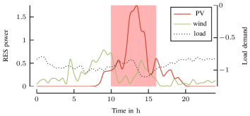
Figure 2: Power profiles of RES and the load demand. The highlighted part shows the CF period between $10.00$ to $16.00$.

The generator parameters were taken from [3] and transformed to per-unit (pu). The weights of the operational cost and the operational limits can be found in Tables I and II. In MPC, the sampling time is $T_{s}=30\,\mathrm{min}$, the prediction horizon is $h=12$ and the discount factor is $\gamma=0.95$. A naive forecaster provides the forecasts for the RES infeed and the load demand of the MG [25]. Finally, the MPC problem is implemented in Matlab^® 2017b with YALMIP [26] and solved with Gurobi 6.5. The analysis was carried out for a simulation period of one day. First, the closed-loop simulation for this period is performed with MPC without occurrence of any CF. The results are labelled as reference in Figures 3 and 4 and Table III. These results serve as reference for the evaluation of the scenarios with CFs.

Simulation with CF

The duration of the CF is selected as $6\,\mathrm{h}$, from $10.00$ to $16.00$, which is highlighted in Figure 2. It can be observed that RES have high infeed during this period and storage units ideally store the excess generation. Two communication failure scenarios are considered in this period:

1. Scenario I : CF at one storage unit - battery at bus $4$.

2. Scenario II : CF at both the storage units.

Closed-loop simulations are carried out for these scenarios with 1) MPC Problem 1, which is referred to as MPC and 2) MPC Problem 2 which is referred to as enhanced MPC. The energy of the batteries in scenario I and scenario II is shown in Figure 3 and Figure 4. The energy wasted from the RES and energy output from the thermal units during the closed-loop simulation for the above scenarios are summarised in Table III.

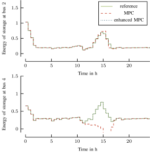
Figure 3: Closed-loop simulations in scenario I: Energy levels of storages with 1) reference 2) MPC 3) enhanced MPC.

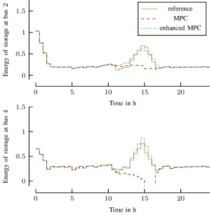
Figure 4: Closed-loop simulations in scenario II: Energy levels of storages with 1) reference 2) MPC 3) enhanced MPC.

In scenario I, the energy of the batteries with enhanced MPC coincides with the reference MPC (without CF). This is empirical evidence that the statement made on open-loop behaviour in Proposition 1 also applies to closed-loop behaviour. In the case with MPC, the storage at bus $4$ cannot be influenced during the CF period and only the storage at bus $2$ is utilised for storing energy. This effect can be noticed in the storage at bus $2$ whose energy level is higher than reference for some periods during the CF. Furthermore, from Table III it can be observed that the wasted RES energy and the thermal energy with both the reference and the enhanced MPC coincide. MPC leads to an increase in RES wastage that is compensated by the thermal units.

In scenario II, the energy of the batteries with enhanced MPC slightly differs from the reference. However, it can be noticed that the energies are close to the reference profile. In the case with MPC both the storages cannot be influenced and therefore their energy profiles deviate from the reference profile. Table III shows that the enhanced MPC results in a slightly increased wastage of RES energy and the thermal energy compared to scenario I. However, these values are lower than the MPC.

TABLE III: RES energy wastage and the thermal energy output in closed-loop simulation

	without CF	scenario I		scenario II
	reference	MPC	enhanced MPC	MPC	enhanced MPC
RES wastage energy ($\mathrm{puh}$)	2.68	3.16	2.68	3.85	2.73
thermal energy ($\mathrm{puh}$)	11.68	12.10	11.68	12.77	11.71

We can conclude that in scenario I, where the CF occurs at only one storage unit, the enhanced MPC results in the same power profiles as the reference. In both scenario I and scenario II, the enhanced MPC has a better performance than the MPC.

VI Conclusion

In this paper, we proposed an MPC formulation for the operation of an MG during communication failure. This formulation takes into account the hierarchical control layers of the MG. This allows to adjust the power output of a unit affected by communication failure. In particular, we formulated the problem when the communication failure occurs in storage units. In this case, we also discuss the estimation of the current energy level of the battery with communication failure. Finally, we show the benefits of the proposed approach with a numerical example.

The proposed approach assumes only communication failures and therefore a possible extension is to include electrical failures. Also, the current approach does not account for uncertainties in the forecasts and possible future communication failures. Including them in a robust framework is another future direction.

References

- [1] REN21 Secretariat, “Renewables 2018 global status report,” REN21, Paris, France, Tech. Rep., 2018.
- [2] Department of Energy Office of Electricity Delivery and Energy Reliability, “2012 DOE microgrid workshop summary report,” Department of Energy Office of Electricity Delivery and Energy Reliability, Tech. Rep., 2012.
- [3] A. Parisio, E. Rikos, and L. Glielmo, “A model predictive control approach to microgrid operation optimization,” IEEE Transactions on Control Systems Technology, vol. 22, no. 5, pp. 1813–1827, Sep. 2014.
- [4] L. E. Sokoler, P. J. Dinesen, and J. B. Jørgensen, “A hierarchical algorithm for integrated scheduling and control with applications to power systems,” IEEE Transactions on Control Systems Technology, vol. 25, no. 2, pp. 590–599, March 2017.
- [5] C. A. Hans, P. Sopasakis, J. Raisch, C. Reincke-Collon, and P. Patrinos, “Risk-averse model predictive operation control of islanded microgrids,” 2019, accepted for publication in the IEEE Transactions on Control Systems Technology. [Online]. Available: https://arxiv.org/abs/1809.06062
- [6] J. Gao, Y. Xiao, J. Liu, W. Liang, and C. P. Chen, “A survey of communication/networking in smart grids,” Future Generation Computer Systems, vol. 28, no. 2, pp. 391–404, 2012.
- [7] B. Falahati, Y. Fu, and L. Wu, “Reliability assessment of smart grid considering direct cyber-power interdependencies,” IEEE Transactions on Smart Grid, vol. 3, no. 3, pp. 1515–1524, Sep. 2012.
- [8] R. Siqueira de Carvalho and S. Mohagheghi, “Analyzing impact of communication network topologies on reconfiguration of networked microgrids, impact of communication system on smart grid reliability, security and operation,” in 2016 North American Power Symposium (NAPS), Sep. 2016, pp. 1–6.
- [9] F. Aminifar, M. Fotuhi-Firuzabad, M. Shahidehpour, and A. Safdarian, “Impact of wams malfunction on power system reliability assessment,” IEEE Transactions on Smart Grid, vol. 3, no. 3, pp. 1302–1309, Sep. 2012.
- [10] B. Moussa, P. Akaber, M. Debbabi, and C. Assi, “Critical links identification for selective outages in interdependent power-communication networks,” IEEE Transactions on Industrial Informatics, vol. 14, no. 2, pp. 472–483, Feb 2018.
- [11] B. Falahati, A. Kargarian, and Y. Fu, “Impacts of information and communication failures on optimal power system operation,” in 2013 IEEE PES Innovative Smart Grid Technologies Conference (ISGT), Feb 2013, pp. 1–6.
- [12] A. Zidan, M. Khairalla, A. M. Abdrabou, T. Khalifa, K. Shaban, A. Abdrabou, R. El Shatshat, and A. M. Gaouda, “Fault detection, isolation, and service restoration in distribution systems: State-of-the-art and future trends,” IEEE Transactions on Smart Grid, vol. 8, no. 5, pp. 2170–2185, Sep. 2017.
- [13] I. Prodan, E. Zio, and F. Stoican, “Fault tolerant predictive control design for reliable microgrid energy management under uncertainties,” Energy, vol. 91, pp. 20 – 34, 2015.
- [14] J. Zhang and E. Modiano, “Joint frequency regulation and economic dispatch using limited communication,” in 2018 IEEE International Conference on Communications, Control, and Computing Technologies for Smart Grids (SmartGridComm), Oct 2018, pp. 1–6.
- [15] K. Paridari, N. O’Mahony, A. El-Din Mady, R. Chabukswar, M. Boubekeur, and H. Sandberg, “A framework for attack-resilient industrial control systems: Attack detection and controller reconfiguration,” Proceedings of the IEEE, vol. 106, no. 1, pp. 113–128, Jan 2018.
- [16] D. M. de la Peña and P. D. Christofides, “Lyapunov-based model predictive control of nonlinear systems subject to data losses,” IEEE Transactions on Automatic Control, vol. 53, no. 9, pp. 2076–2089, 2008.
- [17] G. Franzè, F. Tedesco, and D. Famularo, “Model predictive control for constrained networked systems subject to data losses,” Automatica, vol. 54, pp. 272 – 278, 2015.
- [18] T. L. Vandoorn, J. C. Vasquez, J. De Kooning, J. M. Guerrero, and L. Vandevelde, “Microgrids: Hierarchical control and an overview of the control and reserve management strategies,” IEEE Industrial Electronics Magazine, vol. 7, no. 4, pp. 42–55, Dec 2013.
- [19] A. M. Kosek, G. T. Costanzo, H. W. Bindner, and O. Gehrke, “An overview of demand side management control schemes for buildings in smart grids,” in 2013 IEEE International Conference on Smart Energy Grid Engineering (SEGE), Aug 2013, pp. 1–9.
- [20] A. Krishna, J. Schiffer, and J. Raisch, “A consensus-based control law for accurate frequency restoration and power sharing in microgrids in the presence of clock drifts,” in 2018 European Control Conference (ECC), June 2018, pp. 2575–2580.
- [21] B. Stott, J. Jardim, and O. Alsac, “Dc power flow revisited,” IEEE Transactions on Power Systems, vol. 24, no. 3, pp. 1290–1300, Aug 2009.
- [22] B. Eldridge, R. O’Neill, and A. Castillo, “An improved method for the dcopf with losses,” IEEE Transactions on Power Systems, vol. 33, no. 4, pp. 3779–3788, July 2018.
- [23] M. Živić Đurović, A. Milačić, and M. Kršulja, “A simplified model of quadratic cost function for thermal generators,” Ann. DAAAM 2012 Proc. 23 Int. DAAAM Symp., vol. 23, no. 1, pp. 25–28, 2012.
- [24] Atmospheric Radiation Measurement Climate Research Facility. Surface Meteorology System. June 2009–Oct. 2009, 5’ 28" N, 1’ 45" W: Eastern North Atlantic Facility, windspeed. ARM Data Archive: Oak Ridge, TN, USA. Data set accessed 2011-07-14 at www.arm.gov.
- [25] R. J. Hyndman and G. Athanasopoulos, Forecasting: principles and practice. OTexts, 2018.
- [26] J. Löfberg, “YALMIP: A toolbox for modeling and optimization in MATLAB,” in IEEE CACSD, 2004, pp. 284–289.