The Spectral Energy Distributions of Active Galactic Nuclei

Abstract

We present spectral energy distributions (SEDs) of 41 active galactic nuclei, derived from multiwavelength photometry and archival spectroscopy. All of the SEDs span at least 0.09 to $30~{}{\rm\mu m}$, but in some instances wavelength coverage extends into the X-ray, far-infrared and radio. For some AGNs we have fitted the measured far-infrared photometry with greybody models, while radio flux density measurements have been approximated by power-laws or polynomials. We have been able to fill some of the gaps in the spectral coverage using interpolation or extrapolation of simple models. In addition to the 41 individual AGN SEDs, we have produced 72 Seyfert SEDs by mixing SEDs of the central regions of Seyferts with galaxy SEDs. Relative to the literature, our templates have broader wavelength coverage and/or higher spectral resolution. We have tested the utility of our SEDs by using them to generate photometric redshifts for $0<z\leq 6.12$ AGNs in the Boötes field (selected with X-ray, IR and optical criteria) and, relative to SEDs from the literature, they produce comparable or better photometric redshifts with reduced flux density residuals.

1 Introduction

Templates or models of active galactic nucleus (AGN) spectral energy distributions (SEDs) can be critical for k-corrections, exposure time calculations, modelling quasar selection, modelling the emission from quasars and photometric redshifts, (e.g. see the review of AGN photometric redshifts of Salvato et al., 2018). While AGN SEDs are sometimes described as power-laws, there are several continuum features that can impact broadband photometry, including the big blue bump, a $\sim 1~{}{\rm\mu m}$ inflection attributed to changing contributions from the disk and torus, and mid-infrared features from silicate emission (e.g., Elvis et al., 1994; Haas et al., 2005; Shang et al., 2005; Netzer et al., 2007, and references therein). Emission lines can also be sufficiently strong in Type 1 AGNs to impact broadband photometry. For example, at $z>3.5$ the broad ${\rm H\alpha}$ emission of Type 1 quasars can shift their observed colours towards and away from the locus of galaxy colours (e.g., Richards et al., 2001; Cool et al., 2006). While complicating quasar selection and k-corrections, these spectral features are of utility for photometric redshifts.

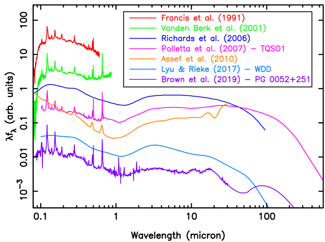
Figure 1: Illustrative examples of quasar spectral energy distributions from the past two decades (Francis et al., 1991; Vanden Berk et al., 2001; Richards et al., 2006; Polletta et al., 2007; Assef et al., 2010; Lyu & Rieke, 2017), along with our SED for PG 0052+251. These templates were created using different methods and with different purposes, so some caution is required directly comparing them. However, the trend towards improved wavelength coverage and spectral resolution is evident. Apart from the improved spectral resolution, our SED for PG 0052+251 shows prominent mid-infrared silicate emission features (also see Netzer et al., 2007) and a peak at $\sim 100~{}{\rm\mu m}$ caused by thermal emission by dust.

AGN SEDs with broad wavelength coverage have been created by combining spectroscopy and/or photometry of many individual quasars, and exploiting the broad observed redshift range of quasars (e.g., Francis et al., 1991; Elvis et al., 1994; Vanden Berk et al., 2001; Polletta et al., 2007; Salvato et al., 2009; Assef et al., 2010; Hsu et al., 2014; Selsing et al., 2016). As Figure 1 illustrates, this approach can produce high signal-to-noise mean spectra and principal components. A risk is the composite spectra may not correspond to any individual quasar, and the principal components can produce unphysical spectra (i.e., when used to model noisy photometry), although in practice such SEDs can approximate individual quasars. SEDs produced using photometry of many quasars understandably have low resolution, and this can result in significant spectral features being absent from AGN SED templates. For example, the diversity seen in Spitzer IRS mid-infrared spectroscopy of quasars (e.g., Haas et al., 2005; Netzer et al., 2007; Lyu et al., 2017) is largely absent from composite quasar SEDs, with most SEDs in Figure 1 not showing the two silicate emission features seen in the SED of PG 0052+251.

The alternative to composite AGN SED templates is photometry and spectrophotometry of individual objects. This approach has been used for over 50 years, with the wavelength range, precision and spectral resolution of AGN SEDs improving over that time (e.g., Oke, 1963; Oke et al., 1970; de Bruyn & Sargent, 1978; Edelson & Malkan, 1986; Shang et al., 2005; Hernán-Caballero et al., 2016). Spectrophotometry of individual AGNs has expanded from optical spectrophotometry into the UV, near-IR and mid-IR (e.g., Shang et al., 2005; Landt et al., 2008; Hernán-Caballero et al., 2016). However, while spectrophotometry does exist of individual quasars between $0.1$ and $30~{}{\rm\mu m}$, there have been no SEDs of individual quasars that use spectrophotometry to span this whole wavelength range (although photometric SEDs with broad wavelength coverage have been available for decades; e.g., Edelson & Malkan, 1986; Elvis et al., 1994; Spinoglio et al., 2002). A significant hurdle is the lack of spectrophotometry of AGNs in the observed $1$ to $2.5~{}{\rm\mu m}$ range, although there are some notable exceptions (e.g., Glikman et al., 2006; Riffel et al., 2006; Landt et al., 2008, 2013).

Relative to spectrophotometry of galaxies, the construction of AGN SEDs offers some advantages and challenges. For sufficiently luminous quasars, emission across much of the electromagnetic spectrum is effectively from a point source, mitigating issues associated with varying (extraction) aperture bias as a function of wavelength. However, quasar variability means spectra taken years (or months) apart may not measure the same flux density at a given wavelength, and the strength and width of emission lines may have changed (e.g., Matthews & Sandage, 1963; Hook et al., 1994; Soldi et al., 2008; Simm et al., 2016). While stellar population models (e.g., Bruzual & Charlot, 2003; da Cunha et al., 2008) can be used to cover gaps in spectral coverage for galaxies (e.g., Brown et al., 2014b), quasar spectra have emission lines and continuum features that aren’t always trivial to model (particularly if photometry as a function of wavelength is impacted by variability).

In this paper we present SEDs of 41 individual AGNs created by combining archival spectrophotometry spanning broad wavelength ranges. All of the AGN SEDs span $0.09$ to $30~{}{\rm\mu m}$, but in some instances SEDs have been expanded into the X-ray, far-infrared and radio. Our goal is to provide SEDs that have higher resolution and greater precision than existing libraries. However, clear risks include variability and wavelength dependent aperture bias introducing wavelength dependent errors. We thus test the utility of our SEDs to produce accurate photometric redshifts and quantify their performance using several metrics (e.g. redshift errors and flux density residuals).

The structure of this paper is as follows. In Section 2 we describe the input spectroscopy, photometry and models used for the SEDs. We describe the construction of the SEDs in Section 3, including rescaling the input spectra and models to produce continuous SEDs, and the production of Seyfert SEDs using combinations of AGN and host galaxy SEDs. In Section 4 we provide an overview of the SEDs, including their restframe colours and observed colours as a function of redshift. We discuss the utility of the SEDs for photometric redshifts in Section 5, including comparison with other SED template libraries and quantification of photometric redshift performance (e.g. flux density residuals). We provide the principal conclusions of this work in Section 6. Throughout this paper we use AB magnitudes and a flat cosmology with $\Omega_{m}=0.3$ and $H_{0}=70~{}{\rm km~{}s^{-1}~{}Mpc^{-1}}$.

2 Input data and models

2.1 Spectrophotometry

Our AGN sample was selected based on the availability of spectrophotometry spanning the 0.1 and $30~{}{\rm\mu m}$ wavelength range, although some AGNs have gaps in this wavelength range while others have X-ray and far-infrared spectra. We draw heavily on ground-based optical and near-infrared spectroscopy from Shang et al. (2005), Riffel et al. (2006), Landt et al. (2008) and Landt et al. (2013). At other wavelengths we utilise spectrophotometry from the Nuclear Spectroscopic Telescope Array (NuSTAR), Suzaku, XMM-Newton, the Chandra X-ray observatory, the Far Ultraviolet Spectroscopic Explorer (FUSE), the Hopkins Ultraviolet Telescope (HUT), the International Ultraviolet Explorer (IUE), the Wisconsin Ultraviolet Photo-Polarimeter Experiment (WUPPE), the Galaxy Evolution Explorer (GALEX), Hubble Space Telescope (HST), Akari, Spitzer, the Infrared Space Observatory (ISO) and Herschel. Given our extensive use of archival spectra, our sample has significant overlap with existing studies and compilations of AGN spectra and SEDs including AGN Watch (Peterson, 1999), FOSAGN (Evans & Koratkar, 2004) and studies exploiting Akari and Spitzer spectroscopy (e.g., Shi et al., 2014; Kim et al., 2015).

Selecting AGNs on the basis of available multi-wavelength spectrophotometry results in a sample biased towards relatively bright and well studied broadline AGNs. Furthermore, as we want to create continuous spectrophotometry taken with a variety of instruments, we tend to favour bright quasars or nearby galaxy nuclei that are dominated by AGN light, as aperture bias hinders making SEDs of objects where the spectra are complex blends of AGN and host galaxy light. The issue of aperture bias is highlighted by the variety of extraction apertures used, which include the IUE $20^{\prime\prime}\times 10^{\prime\prime}$ elliptical aperture, HST STIS slits that vary between 0.05 to $2^{\prime\prime}$ width, the SDSS $3^{\prime\prime}$ diameter fibre, and Spitzer IRS low resolution spectroscopy slits that are $3.6^{\prime\prime}$ and $10.6^{\prime\prime}$ wide (short and long of $14~{}{\rm\mu m}$).

Our requirement for multi-wavelength spectrophotometry biases us against obscured AGNs that mostly lack ultraviolet spectrophotometry and/or have significant host galaxy contributions to the spectrum at wavelengths short of $3~{}{\rm\mu m}$. To mitigate but not eliminate this bias we include some obscured AGNs that lack spectrophotometry between 0.1 and $30~{}{\rm\mu m}$, replacing the missing spectrophotometry with simple empirical models.

Our final sample consists of 41 AGNs, whose basic properties are summarised in Table 1. Our use of archival data results in us using spectra from a large number of archives and papers that are detailed in Table 2. In some instances we have used the spectra as published in papers whereas in other instances we have used more recent reductions provided by archives including the Combined Atlas of Sources with Spitzer IRS Spectra (CASSIS; Lebouteiller et al., 2011), the Barbara A. Mikulski Archive for Space Telescopes (MAST) and the Hubble Spectral Legacy Archive (HSLA; Peeples et al., 2017)

Table 1: The basic properties of the sample and the SED wavelength ranges.

Name	Coordinates		$z$	$m_{g}$	$M_{g}$	$E(B-V)$	Phot.	AGN	${\rm EW(H\alpha+[NII])}$	SED $\lambda$	Scale
	(J2000)					(mag)	Aper.	Class†	(Å)	range (${\rm\mu m}$)	range
2MASX J130005…	195.0223	16.5374	0.0799	17.0	-20.8	0.02	$10^{\prime\prime}$	S1i	62	$9.0\times 10^{-2}-6.4\times 10^{1}$	$1.0-2.5$
3C 120	68.2962	5.3543	0.0330	13.5	-21.8	0.36	$10^{\prime\prime}$	S1.5	817	$1.0\times 10^{-5}-4.8\times 10^{6}$	$1.0-1.7$
3C 273	187.2779	2.0524	0.1583	12.8	-26.4	0.03	$10^{\prime\prime}$	S1.0	446	$9.0\times 10^{-6}-3.4\times 10^{6}$	$0.9-1.2$
3C 351	256.1724	60.7418	0.3719	15.3	-25.8	0.02	$10^{\prime\prime}$	S1.5	349	$9.9\times 10^{-5}-7.1\times 10^{6}$	$0.5-1.4$
3C 390.3	280.5375	79.7714	0.0561	14.9	-21.7	0.09	$10^{\prime\prime}$	S1.5	1441	$1.0\times 10^{-5}-9.5\times 10^{6}$	$0.5-25$
Ark 120	79.0475	-0.1498	0.0327	13.6	-22.1	0.12	$10^{\prime\prime}$	S1.0	529	$2.0\times 10^{-5}-2.9\times 10^{5}$	$0.8-4.0$
Ark 564	340.6639	29.7254	0.0247	14.5	-20.5	0.06	$10^{\prime\prime}$	S3	197	$8.8\times 10^{-2}-3.6\times 10^{1}$	$0.8-1.2$
Fairall 9	20.9407	-58.8058	0.0470	13.9	-22.3	0.02	$10^{\prime\prime}$	S1.2	574	$2.5\times 10^{-5}-9.6\times 10^{2}$	$0.6-2.1$
F2M1113+1244	168.4777	12.7443	0.6812	20.7	-23.4	0.02	$10^{\prime\prime}$	S1	430	$9.0\times 10^{-2}-3.5\times 10^{1}$	$0.5-1.0$
H 1821+643	275.4888	64.3434	0.2968	14.2	-26.6	0.05	$10^{\prime\prime}$	S1.2	636	$7.0\times 10^{-2}-1.5\times 10^{6}$	$1.0-1.2$
IRAS 11119+3257	168.6620	32.6926	0.1876	18.6	-21.8	0.02	$10^{\prime\prime}$	S1n	370	$9.0\times 10^{-2}-4.2\times 10^{2}$	$1.0-1.2$
IRAS F16156+0146	244.5392	1.6559	0.1320	18.5	-20.3	0.08	$10^{\prime\prime}$	S2	511	$9.0\times 10^{-2}-3.3\times 10^{1}$	$0.9-2.3$
Mrk 110	141.3035	52.2862	0.0353	15.8	-21.0	0.01	$10^{\prime\prime}$	S1n	917	$2.0\times 10^{-5}-3.6\times 10^{1}$	$0.6-8.0$
Mrk 1502	13.3956	12.6934	0.0589	14.2	-22.8	0.08	$10^{\prime\prime}$	S1n	346	$8.5\times 10^{-2}-2.9\times 10^{5}$	$0.6-2.0$
Mrk 231	194.0593	56.8737	0.0422	13.7	-22.4	0.01	$10^{\prime\prime}$	S1.0	293	$4.4\times 10^{-5}-9.6\times 10^{6}$	$0.9-2.0$
Mrk 279	208.2644	69.3082	0.0305	14.3	-21.6	0.02	$10^{\prime\prime}$	S1.0	242	$1.0\times 10^{-5}-9.7\times 10^{2}$	$0.9-2.1$
Mrk 290	233.9683	57.9026	0.0302	15.0	-20.1	0.01	$10^{\prime\prime}$	S1.5	303	$1.0\times 10^{-5}-3.6\times 10^{1}$	$1.0-1.1$
Mrk 421	166.1138	38.2088	0.0300	13.4	-22.3	0.02	$10^{\prime\prime}$	HP	-	$1.0\times 10^{-5}-3.6\times 10^{1}$	$1.0-2.9$
Mrk 493	239.7901	35.0299	0.0310	15.2	-20.3	0.03	$10^{\prime\prime}$	S1n	226	$8.7\times 10^{-2}-3.6\times 10^{1}$	$1.0-2.0$
Mrk 509	311.0406	-10.7235	0.0344	13.2	-22.3	0.06	$15^{\prime\prime}$	S1.5	621	$1.0\times 10^{-5}-9.7\times 10^{2}$	$1.0-1.2$
Mrk 590	33.6398	-0.7667	0.0261	14.8	-19.9	0.03	$10^{\prime\prime}$	S1.0	43	$4.2\times 10^{-5}-9.8\times 10^{2}$	$0.2-1.5$
Mrk 817	219.0919	58.7943	0.0315	14.3	-21.4	0.01	$10^{\prime\prime}$	S1.5	406	$2.6\times 10^{-5}-1.4\times 10^{6}$	$0.6-1.2$
Mrk 876	243.4882	65.7193	0.1290	14.6	-23.9	0.03	$20^{\prime\prime}$	S1.0	789	$9.0\times 10^{-6}-1.3\times 10^{6}$	$0.6-1.5$
Mrk 926	346.1812	-8.6857	0.0469	15.0	-21.8	0.04	$10^{\prime\prime}$	S1.5	521	$2.0\times 10^{-5}-9.6\times 10^{2}$	$0.5-3.0$
NGC 3227 Central	155.8774	19.8651	0.0039	13.4	-17.1	0.04	$10^{\prime\prime}$	S1.5	547	$2.8\times 10^{-5}-1.0\times 10^{3}$	$0.3-2.0$
NGC 3516 Central	166.6979	72.5686	0.0088	13.3	-19.0	0.04	$10^{\prime\prime}$	S1.5	218	$1.0\times 10^{-5}-9.9\times 10^{2}$	$0.8-2.0$
NGC 4051 Central	180.7901	44.5313	0.0023	13.6	-15.8	0.02	$10^{\prime\prime}$	S1n	182	$1.0\times 10^{-5}-6.9\times 10^{1}$	$0.7-1.2$
NGC 4151 Central	182.6357	39.4057	0.0033	12.9	-18.5	0.02	$10^{\prime\prime}$	S1.5	640	$2.1\times 10^{-5}-1.0\times 10^{3}$	$0.8-1.7$
NGC 5548 Central	214.4981	25.1368	0.0166	14.5	-19.3	0.02	$10^{\prime\prime}$	S1.5	241	$2.7\times 10^{-5}-9.9\times 10^{2}$	$0.2-1.1$
NGC 5728	220.5996	-17.2531	0.0094	13.3	-19.7	0.12	$15^{\prime\prime}$	S1.9	60	$1.0\times 10^{-5}-9.9\times 10^{2}$	$0.2-4.5$
NGC 7469	345.8151	8.8739	0.0163	13.3	-20.6	0.08	$15^{\prime\prime}$	S1.5	289	$3.0\times 10^{-5}-9.9\times 10^{2}$	$0.6-1.9$
OQ 530	214.9441	54.3874	0.1525	15.7	-23.5	0.03	$10^{\prime\prime}$	HP	-	$7.8\times 10^{-2}-6.9\times 10^{1}$	$0.7-1.0$
PG 0026+129	7.3071	13.2677	0.1420	14.9	-24.1	0.08	$10^{\prime\prime}$	S1.2	320	$1.3\times 10^{-5}-3.3\times 10^{1}$	$1.0-2.5$
PG 0052+251	13.7172	25.4275	0.1545	15.4	-23.8	0.06	$10^{\prime\prime}$	S1.2	603	$9.0\times 10^{-6}-8.7\times 10^{2}$	$0.9-1.6$
PG 1211+143	183.5736	14.0536	0.0809	14.2	-23.4	0.03	$10^{\prime\prime}$	S1n	588	$8.5\times 10^{-2}-9.3\times 10^{2}$	$0.5-1.6$
PG 1307+085	197.4454	8.3302	0.1538	15.4	-23.5	0.04	$10^{\prime\prime}$	S1.2	597	$7.9\times 10^{-2}-8.7\times 10^{2}$	$0.5-1.0$
PG 1415+451	214.2534	44.9351	0.1137	16.2	-22.4	0.01	$10^{\prime\prime}$	S1.0	297	$8.3\times 10^{-2}-3.4\times 10^{1}$	$0.4-1.5$
PG 2349-014	357.9838	-1.1537	0.1738	15.4	-23.5	0.05	$10^{\prime\prime}$	S1.2	519	$9.0\times 10^{-6}-4.2\times 10^{6}$	$0.9-1.0$
PKS 1345+12	206.8892	12.2900	0.1205	17.1	-22.0	0.03	$10^{\prime\prime}$	S2	303	$1.3\times 10^{-4}-8.7\times 10^{6}$	$1.0-3.9$
Ton 951	131.9269	34.7512	0.0640	14.4	-22.7	0.05	$10^{\prime\prime}$	S1.0	251	$8.6\times 10^{-2}-9.4\times 10^{2}$	$0.9-1.1$
W Com	185.3820	28.2329	0.1020	15.3	-23.1	0.03	$10^{\prime\prime}$	BL	-	$8.2\times 10^{-2}-9.0\times 10^{1}$	$0.9-2.3$

$\dagger$ Classifications taken from Véron-Cetty & Véron (2010).

Table 2: The sources of spectroscopy used for the SEDs.

Name	Sources of spectra
	$<0.01~{}{\rm\mu m}$	$0.09-0.33~{}{\rm\mu m}$	$0.33-1.0~{}{\rm\mu m}$	$1.0-2.5~{}{\rm\mu m}$	$2.5-5~{}{\rm\mu m}$	$5-42~{}{\rm\mu m}$	$42-500~{}{\rm\mu m}$
2MASX J13000533+1632151		9	9, 14	2	2	1
3C 120	6	9, 12	4, 9	4, 9	2	1
3C 273	6	7	3, 7, 9	3	2	1
3C 351		7	5, 7, 14	5	2	1
3C 390.3	6	9, 10, 12	4, 9	4	2	1
Ark 120	6	10, 11	3, 10	3	2	1
Ark 564		8, 10, 11	5, 10, 16	5		1
Fairall 9	6	12, 13, 18	18	2, 18	2	1
F2M1113+1244			14, 39	2, 39	2	1
H 1821+643		10, 13	3, 27, 34	3	2	1
IRAS 11119+3257			14	2	2	1
IRAS F16156+0146		18	18	18, 30	2	1
Mrk 110	6	9, 11, 12	3, 9	3	2	1
Mrk 1502		10, 11	10, 31, 32, 38	38	2	1
Mrk 231	6	8, 9, 10	36, 40	2, 40	2	1	19, 20, 21
Mrk 279	6	12, 13	5, 12, 41	5	2	1
Mrk 290	6	7	3, 7	3	2	1
Mrk 421	6	13, 22	37			1
Mrk 493		10	5, 10, 14	5		1
Mrk 509	6	7	3, 7	2, 3	2	1
Mrk 590	6	8, 12	3, 14	3	2	1
Mrk 817	6	8, 9, 11, 12	3, 41	3	2	1	24
Mrk 876	6	8, 11, 12	3, 12, 31	3	2	1
Mrk 926	6	11, 12	14, 15, 27	27		1
NGC 3227 Central	6	9, 13	5, 9	5		1	24
NGC 3516 Central	6	7, 9	4, 9, 27	4		1
NGC 4051 Central	6	8, 11, 12	5, 16	5		1
NGC 4151 Central	6	9, 11	5, 9	2, 5	2	1
NGC 5548 Central	6	11, 13, 16	3, 14, 16	3	2	1
NGC 5728	6	12	15, 28	23	2	1
NGC 7469	6	10, 11	5, 10, 15, 29	5	2	1	19, 20, 21
OQ 530		26	14			1
PG 0026+129	6	10, 11, 17	4, 15, 17	2, 4	2	1
PG 0052+251	6	7	4, 7	4	2	1
PG 1211+143		8, 12, 13, 31	4, 12, 31	4	2	1
PG 1307+085		8, 10, 11, 12, 31	4, 14, 31	4	2	1
PG 1415+451		10, 11	5, 14, 33	5	2	1
PG 2349-014	6	7	7, 35	35		1
PKS 1345+12			14	2	2	1
Ton 951		7	3, 7	3	2	1
W Com		25	14			1

1 Spitzer IRS, 2 Akari, 3 Landt et al. (2008), 4 Landt et al. (2013), 5 Riffel et al. (2006), 6 This work, 7 Shang et al. (2005), 8 HSLA (Peeples et al., 2017), 9 STIS, 10 FOS, 11 FUSE, 12 IUE, 13 HUT, 14 SDSS, 15 MUSE, 16 AGN Watch, 17 UVES, 18 XShooter, 19 Herschel SPIRE, 20 Herschel PACS, 21 ISO, 22 WUPPE, 23 SINFONI, 24 MIPS SED, 25 COS, 26 GALEX, 27 BASS (Koss et al., 2017; Lamperti et al., 2017), 28 S7 (Dopita et al., 2015), 29 Kim et al. (1995), 30 Veilleux et al. (1999), 31 Wilkes et al. (1999), 32 Jansen et al. (2000), 33 Modified Kuraszkiewicz et al. (2000), 34 Decarli et al. (2008), 35 Glikman et al. (2006), 36 Rodríguez Zaurín et al. (2009), 37 Smith et al. (2009), 38 Garcia-Rissmann et al. (2012), 39 Glikman et al. (2012), 40 Leighly et al. (2014), 41 Barth et al. (2015)

2.2 X-ray spectra

To increase the utility of the SEDs, we have expanded the SEDs into the X-ray for the 27 objects that were detected by the 70-month catalogue (Baumgartner et al., 2013) of the all-sky survey carried out by the Burst Alert Telescope (BAT, Barthelmy et al., 2005) on-board the Neil Gehrels Swift Observatory (Gehrels et al., 2004).

The bulk of our X-ray spectra come from Ricci et al. (2017), who undertook a detailed broad-band (0.3–150 keV) X-ray spectral analysis of the 836 AGN from the Swift/BAT 70-month survey in the framework of the BAT AGN Spectroscopic Survey (BASS; Berney et al., 2015; Koss et al., 2017; Lamperti et al., 2017). This was done using a variety of models and X-ray spectra from XMM-Newton (Jansen et al., 2001), Chandra (Weisskopf et al., 2000), Swift/XRT (Burrows et al., 2005), Suzaku (Mitsuda et al., 2007) and Swift/BAT. To homogenise the fluxes of the individual X-ray spectra and incorporate them into our SEDs, we have scaled the spectra to agree with the Swift/BAT flux, which was integrated over a period of 70 months, and could therefore be considered as a good indicator of the mean AGN emission. We caution that by scaling to the mean X-ray flux, we do reduce the impact of variability on our SEDs, and single epoch observations of AGNs may show more X-ray variabilty (e.g. a broader spread of X-ray to IR flux ratios) than our SEDs. The ratios between the flux measured by 0.3–10 keV observations and the time-averaged Swift/BAT flux for this sample are found to be in the $\sim 0.4-4.3$ range.

For 16 objects we also include additional X-ray spectra from NuSTAR (Harrison et al., 2013), typically in the 3–40 keV range, with the NuSTAR spectra also being scaled to the Swift/BAT flux produce continuous X-ray spectra. To maximise the signal-to-noise ratio we used the following approach whenever there was overlapping spectral coverage from multiple missions. i) For sources with NuSTAR, XMM-Newton or Suzaku observations we used XMM-Newton (Suzaku) observations in the 0.3–10 keV (0.5–10 keV) range, NuSTAR above 10 keV, up to the energy range in which the background radiation would dominate ($E_{\rm bkg}$). Between $E_{\rm bkg}$ and 150 keV we used Swift/BAT data. ii) For sources with NuSTAR and Swift/XRT observations we used Swift/XRT in the 0.3–3 keV interval, NuSTAR between 3 keV and $E_{\rm bkg}$, and Swift/BAT in the $E_{\rm bkg}$–150 keV range.

In several instances the NuSTAR spectra clearly show the narrow iron K$\alpha$ lines (e.g., Shu et al., 2010), including the spectra of Mrk 590, Mrk 926, NGC 3227 and NGC 5728. The sample also includes very diverse X-ray spectral continuum shapes, with several objects showing ionised absorbers (e.g., NGC 4051, 3C 351; see Tombesi et al., 2013 and references therein), and in one case (NGC 5728, Ricci et al., 2015) Compton-thick obscuration ($N_{\rm\,H}\geq 10^{24}\rm\,cm^{-2}$).

2.3 Modelling far-infrared and radio spectra

Relatively few AGNs in our sample have far-infrared spectrophotometry (see Table 2) and we do have not have any radio spectra with broad frequency coverage. However, as the far-infrared is often dominated by thermal emission from warm dust and radio SEDs are approximately power-laws, we can produce functional SEDs by fitting models to the observed fluxes.

We model the thermal emission from warm dust by fitting greybody curves to published far-infrared photometry (when available) from the Herschel/PACS Point Source Catalogue (HPPSC; Marton et al., 2017), the Herschel/SPIRE Point Source Catalogue (HSPSC; Schulz et al., 2017), the WMAP point source catalogue (Bennett et al., 2013) and the Planck point source catalogue (Planck Collaboration et al., 2016). As we are fitting six (or fewer) photometric data points with a model with four free parameters, some caution is required and all fits to the data are visually inspected.

We have been able to extend some of the SEDs to radio wavelengths using published radio flux density measurements to constrain simple empirical models. The radio portion of the SEDs is not as precise as the SEDs at shorter wavelengths, but will still be useful for some purposes (e.g. modelling the range of infrared flux densities of radio selected quasars). Radio flux density measurements are drawn from the WMAP point source catalogue (Bennett et al., 2013), the Planck point source catalogue (Planck Collaboration et al., 2016), GLEAM (Hurley-Walker et al., 2016), the compilation of Kuehr et al. (1981) and the NASA Extragalactic Database (NED). While the WMAP, Planck and GLEAM flux density measurements are relatively homogeneous, most of the radio flux density measurements come from a variety of sources and some caution is required when modelling the data.

To model radio spectra, we fitted polynomials to log radio flux density as a function log frequency. For 3C 351 and PKS 1345+12 we have used the previously published models of Kuehr et al. (1981) for flux density as a function of wavelength. As the input radio fluxes are inhomogenous we cross checked that we were using (effectively) total flux densities and compared the model fits to the measured flux densities (to search for discontinuities resulting from variability etcetera). In some instances a tight relation between radio flux density and frequency is not evident and we couldn’t model the radio SED. However, in other instances the polynomials are good approximations of the observed flux densities (scatter of $\sim 0.1~{}{\rm dex}$) so we include these models in our AGN SEDs.

2.4 Photometry

To scale individual spectra and cross check the validity of the SEDs, we use matched aperture photometry measured from images taken with GALEX, Swift, SDSS, PanSTARRS, Skymapper, 2MASS, WISE and Spitzer. The photometry was measured using circular apertures with the diameters given in Table 1. Point spread function corrections are applied to the GALEX, WISE and Spitzer photometry, and for the longer wavelengths we also expand the aperture size so the point spread function corrections never exceed a factor of two. For the Swift photometry we apply point source coincidence loss corrections, while cautioning that these will be inaccurate for extended sources (e.g. Brown et al., 2014b). All photometry (and relevant spectra) are corrected for Milky Way foreground dust extinction using the Planck dust maps (Planck Collaboration et al., 2011; Planck Collaboration et al., 2014) and a Fitzpatrick (1999) model.

All $0.1$ to $30~{}{\rm\mu m}$ photometry was measured using the AB magnitude system and the corresponding flux densities were determined using $f_{\nu}\simeq 3631~{}{\rm Jy}\times 10^{-0.4m}$ where $m$ is the apparent magnitude. Consequently our photometry may systematically differ from the default photometry in some bands (e.g. when the default zeropoints are defined using a $f_{\nu}\propto\nu^{2}$ source). The WISE $W4$ band effective wavelength differs from what was measured prior to launch, and we have corrected for this using the methodology described in Brown et al. (2014a). Our photometry is summarised in Table 3.

3 Constructing SEDs

3.1 Combining spectra

Our SEDs are anchored in the publicly available spectra summarised in Table 2. In instances where multiple individual extracted spectra are available, as is often the case for IUE and Akari, we combine the individual spectra together to achieve higher signal-to-noise. The individual spectra are also visually inspected, and we mask strong geocoronal features and atmospheric absorption features.

While we mostly use publicly available reduced spectra in the $0.09$ to $500~{}{\rm\mu m}$ range, we reprocessed archival ESO XShooter and SINFONI spectra. We reduced archival XShooter spectra using version 2.9.3 of the XShooter pipeline (Modigliani et al., 2010) accessed via the Reflex interface, followed by telluric line corrections with molecfit (Smette et al., 2015). Mark Durré kindly reduced SINFONI spectra of NGC 5728 as described in Durré & Mould (2018), using the SINFONI data reduction pipeline (version 2.5.2) accessed through the gasgano interface, with telluric correction and flux calibration from standard stars observed at a similar airmass.

The variability of AGNs, exemplified by changing-look quasars, complicates the production of continuous spectra of individual objects. We are utilising spectra and photometry taken over years (and in some instances decades) and inevitably archival data will produce inconsistent flux densities at some wavelengths. To produce continuous SEDs we take the input spectra and apply multiplicative scalings to mitigate discontinuities resulting from the variety of spectrographs, extraction apertures and AGN variability. Preliminary scalings are estimated by comparing spectra with photometry, but AGN variability and aperture bias results in this producing discontinuities, particularly in the ultraviolet and near-infrared. When input spectra overlap in wavelength, we measure the ratio of the flux densities in the relevant wavelength range, and use this to determine scalings that produce continuous spectra. However, as input spectra can have relatively large random and systematic errors at the extrema of their wavelength ranges, manual inspection and intervention is required to produce continuous spectra. In some instances the shape of input spectra taken at different wavelengths (or by different instruments) is inconsistent and does not approximate a plausible SED (even after rescaling), and the relevant AGN has to be rejected from the sample (e.g., Mrk 3, NGC 1068, NGC 6814, PG 0804+761, PG 1302-102).

The multiplicative scalings applied to the individual spectra are plotted in Figure 2 as a function of wavelength and the range of scalings applied to each object is provided in Table 1. For some of our SEDs the multiplicative scalings alter the input flux densities by tens of percent, but in some instances input and final flux densities differ by more than a factor of 3. As AGN variability increases with decreasing wavelength, the scalings plotted in Figure 2 show more scatter in the ultraviolet than in the mid-infrared. We caution that multiplicative scaling of individual input spectra is a crude approximation, and the variability and aperture bias will have some wavelength dependence within the individual input spectra (e.g., emission lines relative to continuum). For some purposes, users of our SEDs may want to restrict themselves to AGN SEDs with a relatively limited range of multiplicative scalings and review papers describing the sources of the individual spectra (which are provided in Table 2).

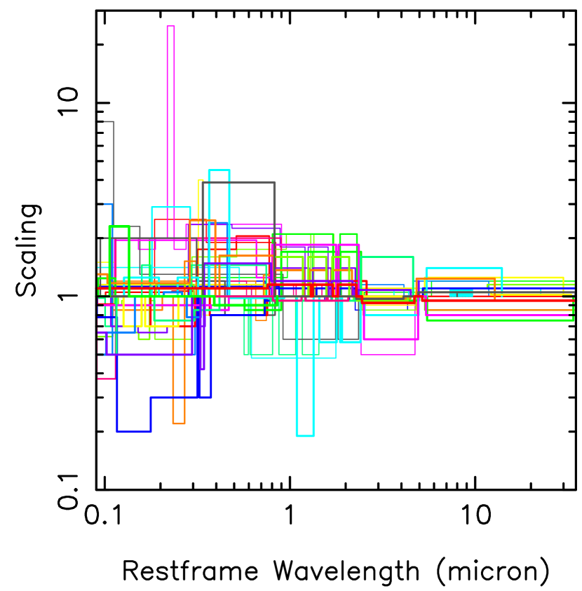
Figure 2: The multiplicative scalings applied to the individual spectra used to produce the AGN SEDs. Variability and aperture bias results in the range of scalings increasing as one moves to shorter wavelengths. For half the sample the scalings never exceed the 0.5 to 2.0 range, but 7 AGNs have scalings that fall outside the 0.33 to 3.0 range (3C 390.3, Ark 120, Mrk 110, Mrk 509, NGC 5548, NGC 5728 and PKS 1345+12).

All of the SEDs have gaps in their spectral coverage, including gaps resulting from atmospheric absorption in the near-infrared, gaps in spectral coverage (i.e., between Akari and Spitzer) and gaps between data and models (i.e., Spitzer and the far-infrared). To interpolate across these gaps we fit polynominals to portions of the spectra on either end of the relevant gap (fitting to log flux density as a function of log wavelength). In some instances we cannot fill (large) gaps in spectral coverage (e.g., X-ray and ultraviolet, far-infrared and radio) so we leave these gaps in the SEDs. When ultraviolet spectra are available but they do not extend down to $0.09~{}{\rm\mu m}$, we extrapolate the ultraviolet using a power-law (fitted to log flux density as a function of log wavelength).

Several obscured quasars, Seyferts and BL Lacs that lack ultraviolet and/or Akari spectra are included in the sample (which would otherwise be completely dominated by broadline quasars). As the Akari spectra are relatively simple (i.e., lacking strong emission lines), we have interpolated across the $2.4$ to $5.5~{}{\rm\mu m}$ wavelength range using polynomials. As BL Lacs are notable for their lack of spectral features and their spectra are almost power-laws, we have used polynomials to interpolate and extrapolate their spectra over large portions of the $0.09$ to $5.5~{}{\rm\mu m}$ wavelength range.

Obscured quasars often show an ultraviolet excess relative to extrapolations of their optical SEDs (i.e., Mrk 231). Consequently, we extrapolate their spectra into a ultraviolet using a toy model, which includes continuum short and long of Lyman-$\alpha$, plus the Lyman-$\alpha$ line itself. The model is deliberately crude so it cannot be confused with data or a physically motivated model, with $f_{\lambda}$ fixed at constant values above and below Lyman-$\alpha$, with Lyman-$\alpha$ emission approximated by a step function. Despite its simplicity, this toy model allows the obscured quasar SEDs to be used when restframe ultraviolet wavelength is required, such as $z>2$ photometric redshifts (although the restframe ultraviolet may be practically undetectable).

In Figure 3 we present a comparison of fluxes synthesised from the 41 SEDs with fluxes measured directly from images. As with the scalings used for the spectra, the difference between synthesised and measured photometry generally increases with decreasing wavelength and there’s an offset at $\sim 1~{}{\rm\mu m}$ resulting from the aperture photometry including host galaxy light. Differences between synthesised and measured fluxes are not a smooth function of wavelength, as we sometimes have multiple photometric measurements taken at similar wavelengths but at different epochs. For example, SDSS, Skymapper and PanSTARRS provide $griz$ photometry while Spitzer and WISE have three bands with comparable effective wavelengths. The flux densities synthesised from the SEDs are provided in Table 4, and these have less variation as a function of wavelength than the directly measured photometry.

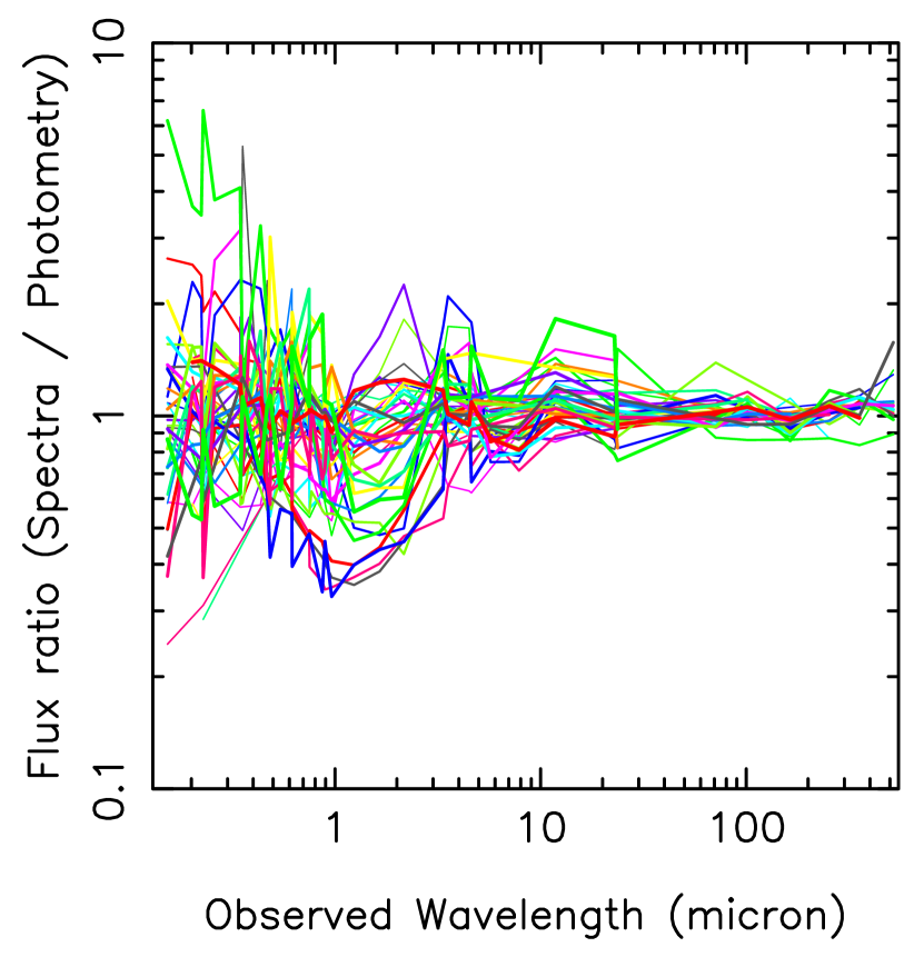
Figure 3: A comparison of measured aperture photometry and photometry synthesised from the SEDs. The photometry includes more host galaxy light than the SEDs, resulting in systematic offsets at $1~{}{\rm\mu m}$, while variability results in increased scatter with decreasing wavelength.

In Figure 1 we provide an illustrative $0.09$ to $600~{}{\rm\mu m}$ SED of a broadline quasar, PG 0052+251, along with illustrative quasar SEDs from the past three decades. The prior literature illustrates the increasing availability of data with time, different methodologies, and compromises one has to make between spectral coverage, spectral resolution and wavelength range. Relative to the prior literature, we have greater spectroscopic coverage, which results in more emission lines and mid-IR spectral features that were largely absent from previous SEDs. The shape of our PG 0052+251 SED in the mid and far-IR is significantly different from that of most previous quasar templates, but we caution that quasar SEDs show significant diversity at these wavelengths (e.g., Netzer et al., 2007; Lyu et al., 2017; Lyu & Rieke, 2017), a point that we shall return to later in this paper.

In Figure 4 we present the $0.09$ to $35~{}{\rm\mu m}$ SEDs of the 41 individual AGNs, with the SEDs ordered by $u-g$ colour. The similarity of the blue quasar SEDs to each other is apparent, although one can also see differences in the mid-infrared spectra at $\sim 20~{}{\rm\mu m}$. Figure 4 illustrates that we have a relatively limited number of red AGN SEDs, and that our red AGN SEDs often utilise toy models and/or power-law interpolation. The red AGN population also shows considerable diversity, including the strength of ${\rm H\alpha}$ emission and $9.7~{}{\rm\mu m}$ silicate absorption.

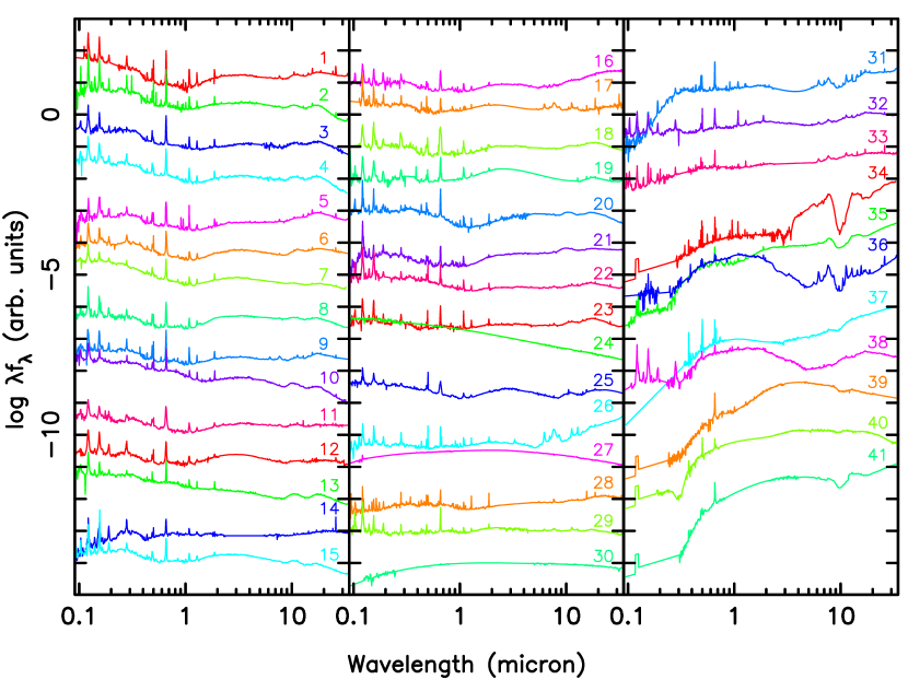
Figure 4: The SEDs of the 41 individual AGNs sorted by restframe $u-g$ colour, with the bluest templates at the top-left of the plot. UV and optical emission lines are immediately evident. The $9.7~{}{\rm\mu m}$ silicate absorption is evident for some red AGN templates while $9.7~{}{\rm\mu m}$ silicate emission can be discerned for some blue quasars. The numbers on the individual SEDs correspond to: 1. 3C 120; 2. Mrk 110; 3. PG 1307+085; 4. PG 0052+251; 5. NGC 4151 Central; 6. H 1821+643; 7. 3C 273; 8. Fairall 9; 9. Mrk 509; 10. PG 0026+129; 11. Mrk 876; 12. PG 2349-014; 13. Ton 951; 14. NGC 3516 Central; 15. Ark 120; 16. Mrk 817; 17. Mrk 493; 18. 3C 390.3; 19. Mrk 926; 20. PG 1211+143; 21. Mrk 1502; 22. Mrk 279; 23. Mrk 290; 24. Mrk 421; 25. 3C 351; 26. NGC 7469; 27. W Com; 28. Ark 564; 29. PG 1415+451; 30. OQ 530; 31. NGC 3227 Central; 32. NGC 5548 Central; 33. NGC 4051 Central; 34. IRAS F16156+0146; 35. Mrk 231; 36, NGC 5728; 37. PKS 1345+12; 38. Mrk 590; 39. F2M1113+1244; 40. 2MASX J13000533+1632151; 41. IRAS 11119+3257.

In Figure 5 we plot the radio to X-ray SEDs for AGNs that have radio coverage. To facilitate comparison of the SEDs, we have normalised them at $1.25~{}{\rm\mu m}$ and overplotted the median radio-loud and radio-quiet SEDs from Elvis et al. (1994), which have been a useful benchmark over the past quarter of a century. Our blue SEDs are similar to those of Elvis et al. (1994), including the factor of $\sim 1000$ difference in radio luminosity for radio-loud and radio-quiet quasars. That said, our SEDs are mostly redder than those of Elvis et al. (1994) in the ultraviolet and optical, and in the far-infrared greybody curves can be steeper than the Rayleigh-Jeans approximation. While many of the radio SEDs are approximately power-laws, 3C 120, 3C 273 and PKS 1345+12 show changes in spectral index at low frequencies (which has been previously noted by White et al., 2018).

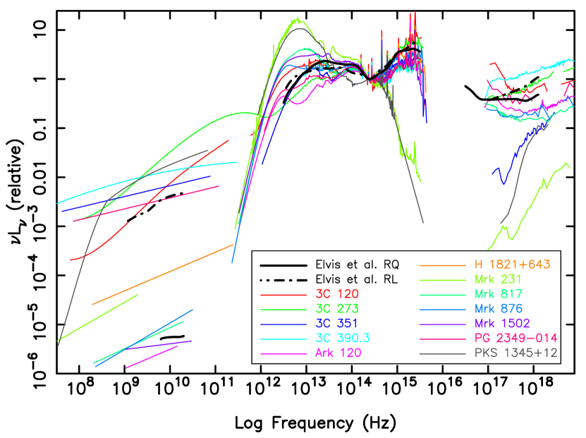
Figure 5: The SEDs of AGNs that have radio coverage, normalised at $1.25~{}{\rm\mu m}$. For comparison we also plot the median radio-loud and radio-quiet SEDs of Elvis et al. (1994). Several features that are evident, including the change of spectral index for 3C 120, 3C 273 and PKS 1345+12 at low frequencies, the diversity of infrared SEDs, and most of our SEDs being redder in the ultraviolet-optical than those of Elvis et al. (1994).

3.2 AGN and host galaxy composites

Our sample is biased towards luminous quasars and the centres of nearby Seyferts where the observed spectrum is dominated by the AGN. We thus do not have many Seyfert galaxies where the fraction of AGN and host galaxy light varies greatly with wavelength, with host galaxy light peaking in the restframe optical and near-infrared. Seyferts comprise the bulk of AGNs detected by many surveys (particularly X-ray selected surveys at low redshift) so the absence of Seyfert templates could hinder the utility of our library, particularly for photometric redshifts (e.g., Salvato et al., 2009; Hsu et al., 2014; Salvato et al., 2018), which is one of the principal motivations for this work.

We have thus created a series of AGN and host galaxy composites to produce Seyfert SEDs. To do this we have taken the AGN SEDs of NGC 3227, 3516, 4051 and 4151 and combined them with the galaxy SEDs of NGC 3310, 4125, 4138, 4569, 4725 and 4826 taken from Brown et al. (2014b). By construction this will produce SEDs that best mimic low redshift AGNs, and a different set of host galaxy SEDs could (or should) be used for Seyferts at higher redshift. As the wavelength coverage and precision of high redshift galaxy SEDs is poor relative to the Brown et al. (2014b) SEDs, we do not create SEDs tailored specifically for high redshift Seyferts for this work. We combine the AGN and $z\sim 0$ host galaxy SEDs by renormalising the spectra at $0.6~{}{\rm\mu m}$ and then summing the SEDs using ratios of AGN to host light spanning from 2:1 to 1:64. This results in 72 additional AGN templates.

4 The colours of AGNs

The synthesised colours of SED templates provide a useful summary of template library properties, including the diversity of the SEDs and differences relative to various object classes and the prior literature. In Figure 6 we present the restframe $ugr$ optical colours of our AGN templates and the local galaxy templates of Brown et al. (2014b). Brown et al. (2014b) used optical scanned spectra, Akari $2.5-4.9~{}{\rm\mu m}$ spectra and Spitzer $5.5-35~{}{\rm\mu m}$ spectra in combination with MAGPHYS models (da Cunha et al., 2008) to produce SEDs for $z<0.04$ galaxies, and Brown et al. (2014b) excluded many powerful AGNs due to the limitations of the version of MAGPHYS used at the time. Bright blue quasars are bluer in $u-g$ than galaxies, but are redder than galaxies in $g-r$ due to the contribution of ${\rm H\alpha}$ to the restframe $r$-band (the ${\rm H\alpha}$ equivalent widths are summarised in Table 1). An extreme example of this is 3C 390.3, which has restframe colours of $u-g=0.1$ and $g-r=0.9$. Reddened AGNs are also offset from the main locus of galaxies, including Mrk 231, which has restframe colours of $u-g=1.2$ and $g-r=0.8$. Extreme examples of reddened AGNs, including F2M 1113+1244 and IRAS 11119+3257, have optical colours unlike those of most red galaxies, including most LIRGS, with restframe $g-r>1$.

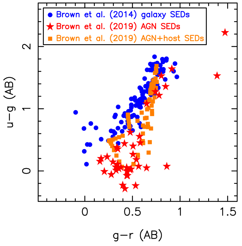
Figure 6: The restframe optical colours of the AGN SED templates (including AGN and host combinations) along with the colours of galaxy SED templates from Brown et al. (2014b). Blue continuum and strong ${\rm H\alpha}$ emission offset templates down and to the right (respectively) from other galaxies.

In Figure 7 we plot the restframe WISE mid-infrared colours of our AGN templates and the galaxy templates of Brown et al. (2014b). There is a locus of quasars that has systematically redder $W1-W2$ colours than most galaxies, and this locus is exploited by a number of mid-infrared quasar selection techniques (e.g., Lacy et al., 2004; Stern et al., 2005; Assef et al., 2013). IRAS F16156+0146 and PKS 1345+12 both have mid-infrared colours significantly redder than most quasars, although in addition to being AGNs these two objects are also ULIRGs. The AGN-host galaxy combinations produce a series of “octopus legs” in Figure 7, connecting the quasar locus with different populations of galaxies.

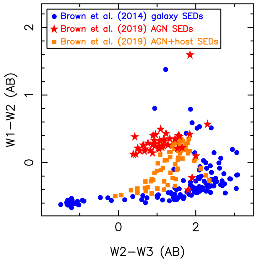
Figure 7: The restframe WISE mid-infrared colours of the AGN SED templates (including AGN and host combinations) along with the colours of galaxy SED templates from Brown et al. (2014b). The AGN templates are clustered in colour-space, and this is exploited by mid-infrared AGN selection criteria (e.g., Lacy et al., 2004; Stern et al., 2005; Assef et al., 2013). AGN and host galaxy combinations form “octopus legs” that branch down towards the bulk of the Brown et al. (2014b) galaxy templates.

The observed colours of SEDs as a function of redshift illustrate how they fill the colour-space and can reveal how individual spectral features impact broadband colours. To benchmark our work, we compare the colours produced by our SEDs to the Brown et al. (2014b) galaxy SEDs, which largely lack powerful AGNs, and the Ananna et al. (2017) galaxy and AGN SEDs, which are a recent iteration of AGN SEDs used for the SWIRE, CDF-S and COSMOS surveys (Polletta et al., 2007; Salvato et al., 2009; Hsu et al., 2014; Ananna et al., 2017). The Ananna et al. (2017) suite of SEDs is also optimised for the wide-field Stripe 82 region, and thus may be directly comparable to our work (i.e. including luminous quasar SEDs).

In Figure 8 we plot observed $u-g$ colour as a function of redshift for the Ananna et al. (2017) galaxy and AGN SEDs, Brown et al. (2014b) galaxy SEDs and the AGN SEDs from this study. There are some obvious similarities between the different template libraries, including a red peak at $z\sim 0.5$ resulting from galaxy (or host galaxy) light. There are clear differences between the template libraries too, including the very blue colours of some of our quasar templates and the contribution of very strong restframe UV emission lines (particularly in 3C and PG quasars) to the $u-g$ colours at $z\sim 1.4$ and $z\sim 2$. The variation of $u-g$ (and $U-B$) quasar colour as a function redshift is well established and produced by some template libraries (e.g., Vanden Berk et al., 2001), it impacts UV-excess quasar selection, and can be exploited for photometric redshifts (e.g., Weinstein et al., 2004)

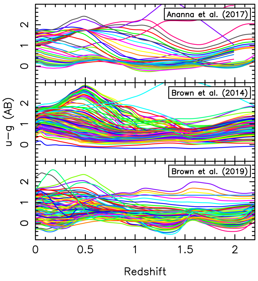
Figure 8: Observed $u-g$ colour as a function of redshift for the Ananna et al. (2017) AGN and galaxy templates, the Brown et al. (2014b) galaxy templates and the AGN templates from this work (including AGN and host combinations). The most notable difference between our templates and the others plotted above are our very blue quasar templates, including contributions by ultraviolet emission lines.

In Figure 9 we plot WISE infrared colours as a function of redshift for the Ananna et al. (2017) SEDs, Brown et al. (2014b) galaxy SEDs, and the AGN SEDs from this study. Low redshift quasars have significantly redder colours than galaxies, and lack strong contributions from the $3.3~{}{\rm\mu m}$ PAH feature and the $1.6~{}{\rm\mu m}$ ${\rm H^{-}}$ spectral feature. We find the WISE $W1-W2$ colours of quasars become gradually bluer with increasing redshift between $z\sim 1.5$ and $z\sim 3$, whereas the colours of galaxies (including some Seyferts) become redder over the same redshift range. At $z\sim 4$ the contribution of ${\rm H\alpha}$ to the WISE $W1$ flux results in very blue $W1-W2$ colours, and is thus a potentially useful feature for photometric redshifts.

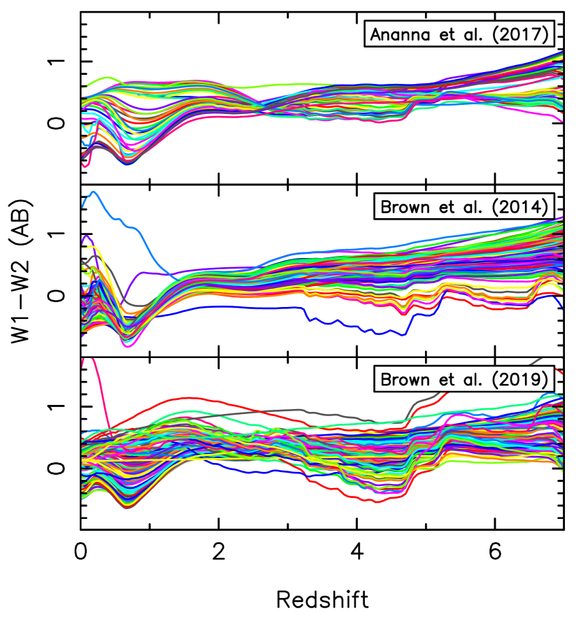
Figure 9: Observed WISE $W1-W2$ colour as a function of redshift for the Ananna et al. (2017) AGN SED templates, the Brown et al. (2014b) galaxy templates and the AGN templates from this work. One clear difference between the mid-infrared colours of our templates and some of those from the literature is evident at $z\sim 4$, where ${\rm H\alpha}$ is in the WISE $W1$ band.

5 Photometric Redshifts

Photometric redshifts (photo-$z$s) are one of the principal motivators for developing our AGN SED library and thus are a natural test of the SEDs validity and utility. Photo-$z$s work particularly well when the objects of interest have a limited range of restframe colours while having observed colours that are a strong function of redshift (exemplified by elliptical galaxies). While UV-excess selected quasars have a limited range of rest-frame optical colours, their mid-infrared SEDs show significant diversity and their colours are a relatively weak function of redshift at $z<2.3$. Thus quasar photo-$z$s have often been a challenge (see the review of Salvato et al., 2018, and references therein).

We test the utility our SEDs for photometric redshifts with AGNs selected from the Boötes field, which we and others have previously used for the development and testing of AGN photometric redshifts (e.g., Brodwin et al., 2006; Duncan et al., 2018a; Duncan et al., 2018b). We utilise the matched aperture photometry initially described by Brown et al. (2007), but then subsequently updated to now include LBT $uy$, Subaru $z$, KPNO 4-m $B_{W}RIJHK_{S}$ and (deeper) Spitzer IRAC photometry. Our AGN sample is selected from the full photometric sample following the three criteria outlined in Duncan et al. (2018a), which expands on the previous work in this field by Hickox et al. (2009). Optical AGNs are selected based on their spectroscopic classification and/or their optical morphology and colours. Infrared selected AGNs are selected using the Spitzer Deep Wide-Field Survey (SDWFS; Ashby et al., 2009) and the Donley et al. (2012) mid-infrared selection criteria. Finally, X-ray AGNs are selected from the XBoötes survey (Murray et al., 2005), a wide-field Chandra survey with (typical) integration times of $5~{}{\rm ks}$ per pointing and an soft X-ray (0.5 to 2 keV) flux limit of $\approx 5\times 10^{-15}$ erg  cm^-2 s^-1.

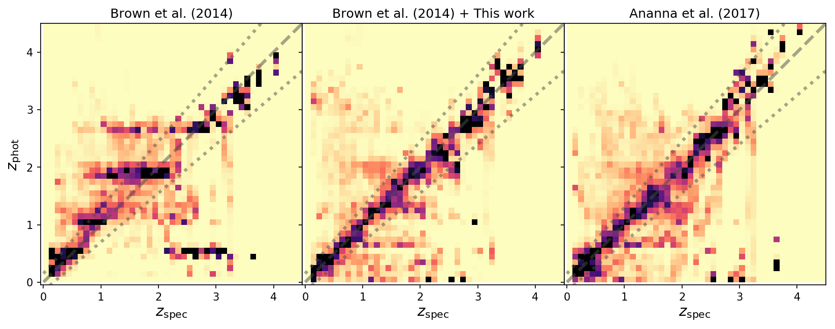
Figure 10: Spectroscopic vs photometric redshift comparison for the Boötes X-ray selected AGN sample at $0<z<4.5$ using three different template sets. Unsurprisingly, Brown et al. (2014b) has the worst performance for AGN photometric redshifts as it (by construction) excludes powerful AGNs. Relative to photometric redshifts determined using the Ananna et al. (2017) templates, photometric redshifts using our new templates have lower $\chi^{2}$ values and slightly better performance.

Limiting the AGN sample to sources with spectroscopic redshifts, our final sample consists of 2058 sources in the redshift range $0<z\leq 6.12$ with a median redshift of $z=1.25$. The bulk of our spectroscopic redshifts come from the MMT AGN and Galaxy Evolution survey (AGES; Kochanek et al., 2012), although some additional redshifts come from Keck, Gemini and other observing programs. As the Boötes field has a $9~{}{\rm deg}^{2}$ area and AGES has an AB magnitude limit of $I=21.9$ for Spitzer IRAC selected AGNs, we have more luminous quasars and Seyferts than deeper surveys of smaller fields.

To compare the utility of our SEDs with prior literature, we have produced three sets of photometric redshifts. We have produced photometric redshifts using 1) the Brown et al. (2014b) SEDs, which do not include luminous AGNs, 2) the AGN and galaxy SED libraries of Ananna et al. (2017) and 3) our new AGN SEDs along with the SEDs of Brown et al. (2014b). Photometric redshifts for each set of templates were determined using EAzY (Brammer et al., 2008). For simplicity, in all cases we apply the same template-fitting approach: using single-template fits only, including the calculation of photometric zero-point offsets, and incorporating an additional 10% flux uncertainty (added in quadrature). We do not apply any magnitude priors when calculating the redshift posteriors at this stage.

When fitting in EAzY, we use the Ananna et al. (2017) templates in a way that best matches their implementation with LePhare (Arnouts et al., 1999) for Stripe 82. Specifically, we apply dust extinction in the range of $0\leq E(B-V)\leq 0.5$ following an SMC-like extinction curve (specifically the parametrisation of Pei, 1992, for this analysis). For the Brown et al. (2014b) templates, when fitted by themselves or when combined with the templates in this work, we apply extinction in the same fashion as for Ananna et al. (2017). However, for the AGN templates added in this work, we use a reduce range of extinction $0\leq E(B-V)\leq 0.2$. For consistency, all templates are interpolated onto the same wavelength grid when dust attenuation is applied.

Formally, the predicted photo-$z$ posterior should account for both the likelihood of a source being a specific galaxy type (or template) at a redshift given the photometry and the prior likelihood of that galaxy type existing at that redshift. Improved photo-$z$ can therefore be gained by accounting for the relative number-density of different galaxy types as a function of redshift; particularly in the case of quasars and AGN where specific types can be extremely rare (e.g. BL Lac objects). This improvement is illustrated by the photo-$z$ quality for X-ray selected AGN gained when removing AGN types typically too rare to be found in deep pencil-beam surveys (e.g., Salvato et al., 2009; Hsu et al., 2014; Salvato et al., 2018). However, we caution that for these tests we have used all of the templates provided and have not attempted to optimise performance using a subset of the templates, therefore minimising any potential systematics that may be induced by the photo-$z$ methodology. We note that the depth of the X-ray survey that provides our primary test sample is well matched to that used in Ananna et al. (2017). We are therefore testing a similar parameter space to that for which the Ananna et al. library has been optimised.

In Figure 10 we present the photometric redshifts of Boötes field X-ray AGNs as a function of spectroscopic redshift. In bins of spectroscopic redshift, we plot the stacked photo-$z$ posteriors (with no additional uncertainty calibration applied) - with the distributions normalised in bins of constant photometric redshift. To improve the visual clarity due to the sparse sample of spectroscopic redshifts at $z_{\textup{spec}}>2$, we stack the posteriors in broader redshift bins than used during template fitting.

Unsurprisingly, as Brown et al. (2014b) does not include powerful AGNs, it performs poorly and has a significant number of catastrophic outliers. All three sets of photometric redshifts show some aliasing, with some erroneous photometric redshifts associated with strong emission lines moving in and out of particular filters. At first glance the photometric redshifts determined with our new templates and the templates of Ananna et al. (2017) are of comparable quality. However, there are some subtler differences such as the templates from this work producing posteriors that are visibly more concentrated around the 1:1 trend at $z>2$. Both the dramatic improvements over the previous Brown et al. (2014b) estimates and the smaller improvements over the Ananna et al. (2017) library are clearer when we investigate the statistical performance as a function of redshift.

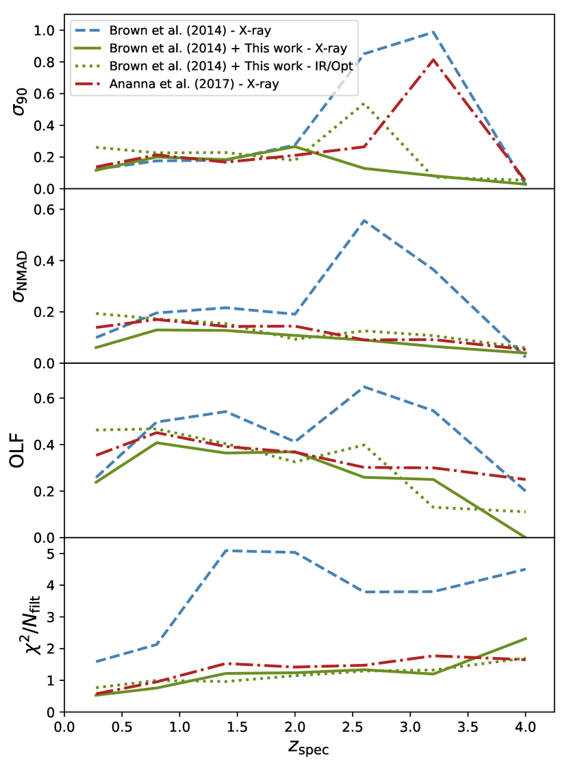
Figure 11: Photometric redshift quality metrics as a function of spectroscopic redshift for the three template sets (see text for metric definitions). Our new AGN SED templates, in combination with the Brown et al. (2014b) galaxy SEDs, produce photometric redshifts for X-ray selected AGNs that are comparable to or better than the photometric redshifts produced using the Ananna et al. (2017) SEDs.

In Figure 11 we plot four metrics of photometric redshift quality: the 90% clipped root mean squared scatter ($\sigma_{90}$), the normalised median absolute deviation ($\sigma_{\textup{NMAD}}$), the outlier fraction (OLF) and median $\chi^{2}$ divided by the number of filters. Our measure of robust scatter, $\sigma_{\textup{NMAD}}$, is defined as $1.48\times\text{median}(\left|\delta z\right|/(1+z_{\text{spec}}))$ as is commonly used within the photo-$z$ literature, where $\delta z=z_{\textup{spec}}-z_{\textup{phot}}$. Similarly, we define the outlier criterion as $\left|\delta z\right|/(1+z_{\textup{spec}})>0.15$. When calculating these metrics, $z_{\textup{phot}}$ is chosen to be the maximum a-posteriori value of the redshift posterior (corresponding to the minimum $\chi^{2}$ given our assumed flat prior). Finally, the bottom panel of Figure 11 shows the median $\chi^{2}/N_{\textup{filt}}$ for sources in each redshift bin to illustrate the overall goodness-of-fit for each template set. For the metrics presented in the top three panels of Figure 11, sources with the worst 5% of $\chi^{2}/N_{\textup{filt}}$ were excluded for each template set.

For all metrics presented in Figure 11, we find our SEDs produce photometric redshifts for $z<2.5$ X-ray AGNs that are comparable to those using the Ananna et al. (2017) SEDs, with improvements for $z>2.5$ AGNs including lower $\sigma_{90}$ and OLF. We also find that our new SEDs are able to perform equally well for mid-infrared and optically selected AGN population - illustrating the wide range of parameter space represented in our SED library. The templates presented in this work are able to produce consistently lower $\chi^{2}$ than either comparison template library, with a median $\chi^{2}/N_{\textup{filt}}\approx 1$ at all $z_{\textup{spec}}$; illustrating that we are able to better represent the observed optical to mid-IR colour space of high redshift AGNs than previous libraries.

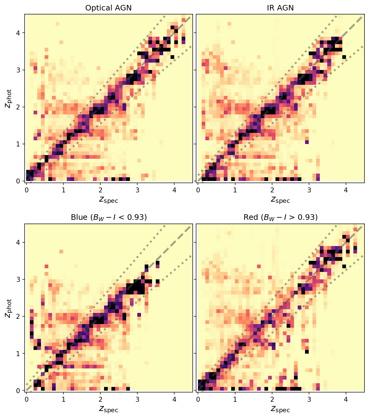
Figure 12: Photometric redshifts, determined with our SEDs, for AGNs that meet optical selection criteria, Spitzer infrared selection criteria, and when separated into blue and red apparent optical colours. As in Figure 10 plot the stacked photo-$z$ posteriors, with the distributions normalised in bins of constant photometric redshift. While photometric redshift performance will inevitably depend on AGN selection and colour (and this can be seen above), the photometric redshift performance is comparable for the four subsamples shown.

As AGN SEDs are a function of both selection criteria and (by definition) colour, we expect photometric redshift performance to also depend on selection criteria and colour. In Figure 12 we present the photometric redshifts, determined with our SEDs, as a function of spectroscopic redshift for AGNs that meet optical selection criteria, Spitzer infrared selection criteria (Donley et al., 2012), an optical blue colour criterion ($B_{W}-I<0.93$) and an optical red colour criterion ($B_{W}-I>0.93$). Overall photometric redshift performance for these different subsets of AGNs is comparable, although red AGN photometric redshifts outperform blue AGN photometric redshifts over certain redshift ranges (and vice versa). We suspect the variation of photometric redshift performance is due to the contribution or absence of strong spectral features such as the 4000 Å  break in AGN host galaxies and the $\sim 1~{}{\rm\mu m}$ inflection in blue quasars SEDs.

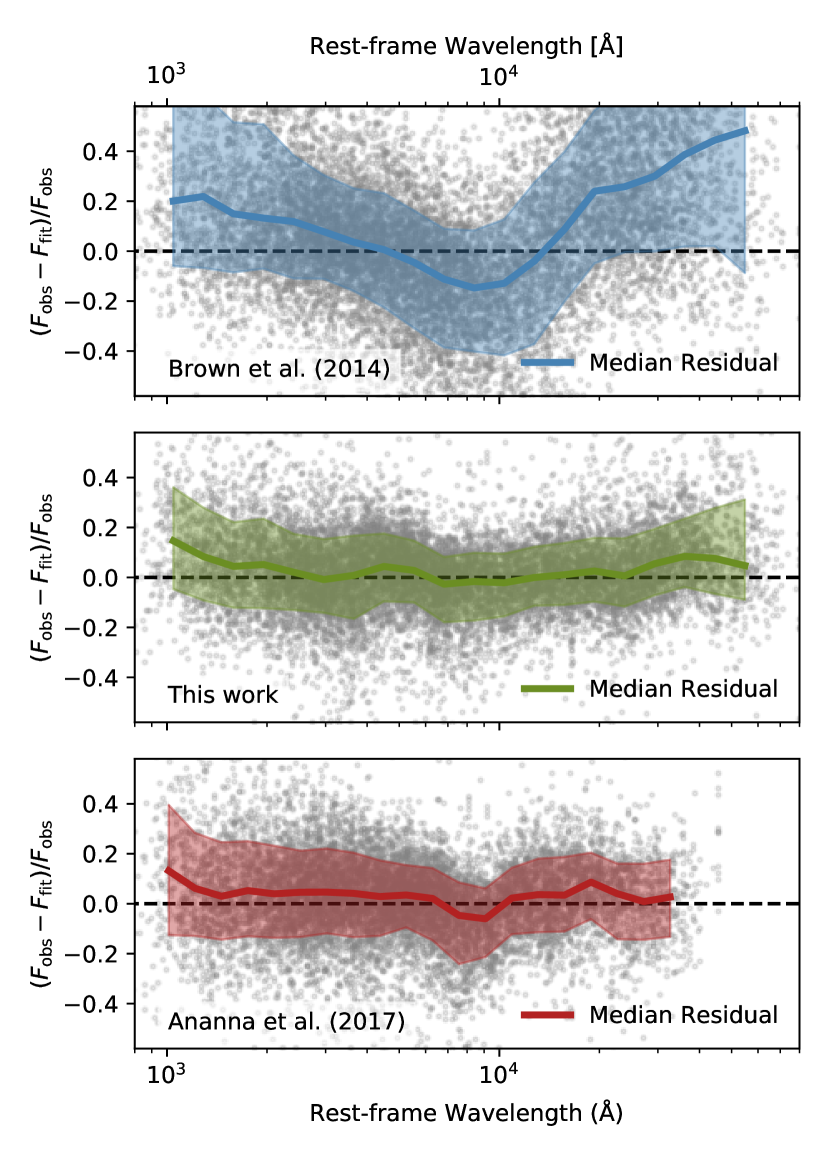
Figure 13: Rest-frame residuals for the template fits (with redshifts are fixed to the known spectroscopic redshift) using each of the three SED libraries employed in this work. Background grey points correspond to individual datapoints (i.e. one for each fitted filter per source) while the solid coloured lines correspond to the median residual within a given wavelength bin and the shaded region corresponds to the 16 and 84th percentiles (i.e., $\pm 1\sigma$). Our AGN SEDs in combination with the Brown et al. (2014b) galaxy SEDs (middle panel) span a broad wavelength range while producing small residuals, with just 3% of the residuals being $3\sigma$ outliers.

To further illustrate how our new library is able to better represent the panchromatic colours of the observed AGN population, in Figure 13 we show the rest-frame residual fitting errors when the redshifts are fixed to the known spectroscopic redshift for our full AGN sample. Compared to the Brown et al. (2014b) library alone, biases in the model colours are reduced by a factor of $\sim 2$ to 5 depending on the rest-frame wavelength. The scatter in residual colours is also significantly reduced for the SEDs provided in this work compared to both the Brown et al. (2014b) and Ananna et al. (2017); indicative of reduced model uncertainties. Over rest-frame wavelengths of $0.1$ to $3~{}{\rm\mu m}$, the median absolute residual reduces from 18% for the Brown et al. (2014b) library to 9% for the combined empirical library of this work. The Ananna et al. (2017) SEDs have median absolute residual of 11%, which is only slightly higher than our work although the Ananna et al. (2017) SEDs are fitted to a more limited wavelength range.

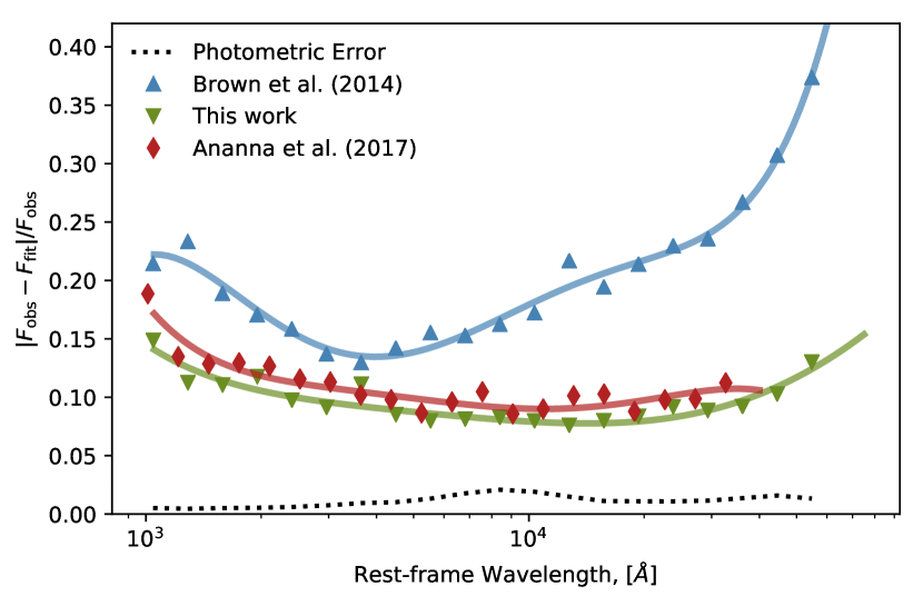
Figure 14: The template error function for each set of template SEDs (solid coloured lines), calculated by subtracting in quadrature the scaled average fractional error (black dotted line) from the median absolute rest-frame residuals (coloured symbols).

In Figure 14 we highlight this reduction in model uncertainties by plotting the ‘template error function’ as presented in Brammer et al. (2008) for each set of SEDs. For each set of SEDs we calculate the template error function by subtracting the scaled average fractional error from the median absolute rest-frame residual (in quadrature). We find that for all three sets of template SEDs, the template error is highest for rest-frame UV and mid-IR emission - consistent with the pattern observed in Brammer et al. (2008) for normal galaxies. In Brammer et al. (2008), the increased uncertainty in these regimes is attributed to intrinsic variation in dust attenuation curves in restframe ultraviolet and the lack of mid-infrared emission from dust in their templates (our SEDs include include mid-infrared emission from dust and, where applicable, PAHs).

The template error estimated from the fits incorporating the AGN SEDs in this work is largely comparable to that of the Ananna et al. (2017) library. As seen in Figure 14, the improvement in overall residuals discussed above can be attributed to improvement in the templates at rest-frame wavelengths of $<2000\textup{\AA}$ and at $\sim 1~{}{\rm\mu m}$. Additionally, the substantial reduction in template error at $\lambda>1~{}{\rm\mu m}$ relative to that of the Brown et al. (2014b) library alone ($2\times$ lower) further illustrates how our new SEDs are able to better represent the observed range of mid-IR colours of AGNs.

As illustrated by Brammer et al. (2008), the inclusion of the template error function when performing template fits (added in quadrature to the flux measurement errors) can yield improvements in the photo-$z$ estimates. To verify that incorporating more realistic model uncertainties in the template fitting leads to further improvement in the photo-$z$s, we calculate a new set of estimates incorporating the template error function specific to each SED library (as presented in Figure 14). Additionally, we also incorporate a simple magnitude dependent prior using the observed $3.6\mu\textup{m}$ Spitzer IRAC magnitude (following the method outlined in Duncan et al., 2018a). For the semi-‘optimised’ photo-$z$ estimates using the extended SED library of this work, we find that the robust scatter reduces from $\sigma_{\textup{NMAD}}=0.12$ to $\sigma_{\textup{NMAD}}=0.095$ across all AGN types, while the overall outlier fraction drops substantially from 37% to 31%.

An exhaustive optimisation of the template fitting method for our AGN test sample is beyond the scope of this work and will be explored further in future studies. However, the improvements gained from the minor changes outlined above illustrate the potential for further dramatic improvements in both precision and reliability. For example, as demonstrated in the works of Polletta et al. (2007), Salvato et al. (2009), Hsu et al. (2014) and Ananna et al. (2017), it is useful to account for the optical morphology of the source when choosing template libraries (e.g. excluding pure quasar SEDs for extended morphologies). Similarly, applying an absolute magnitude prior can prevent severe degeneracies between different SEDs that would otherwise result in unphysical luminosities. Finally, given a particular scientific goal or target sample of interest, the exact subset of templates included in the fit or the range of dust attenuation allowed could be tuned based on our prior knowledge.

6 Conclusions

We have determined the $0.09$ to $30~{}{\rm\mu m}$ SEDs of 41 individual AGNs using a combination of archival spectroscopy, matched aperture photometry and models. In some instances the SEDs have been expanded into the X-ray, far-infrared and radio using combinations of archival spectroscopy, greybody models and simple empirical models. We have also produced 72 additional SEDs that mimic Seyferts, by combining central SEDs of nearby Seyferts with galaxy SEDs from Brown et al. (2014b). All of the SEDs are available via DOI 10.17909/t9-3dbt-8734.

To produce continuous SEDs using archival data taken over years (or decades), we multiplicatively scaled the individual spectra to produce continuous SEDs. For half the AGNs the scalings were between 0.5 and 2.0, but for 7 AGNs the scalings were below 0.33 or above 3. Some gaps in spectral coverage (or between spectra and models) were filled using simple models to interpolate between or extrapolate from the individual spectra. Comparison of the resulting SEDs with matched aperture photometry shows reasonable agreement, with most SEDs agreeing with photometry within a factor of 2. Offsets between the SEDs and photometry decrease with increasing wavelength (as expected given AGN variability) and some offsets are the result of host galaxy light impacting (large) matched aperture photometry.

The overall shapes of our SEDs are similar to those from the prior literature (e.g., Elvis et al., 1994) but we achieve broader wavelength coverage and higher spectral resolution, particularly in the X-ray, mid-infrared and far-infrared. For example, silicate emission features and far-infrared emission from warm dust are evident in our quasar templates. Optical and mid-infrared colours synthesised from our SEDs can differ significantly from those generated by galaxy and AGN SED libraries from the prior literature.

We tested the utility and precision of our AGN SEDs by using them to determine photometric redshifts for X-ray, optical and mid-infrared selected AGNs in the Boötes field. AGN photometric redshifts utilising SED libraries without AGNs can have gross redshift errors. AGN photometric redshifts determined with our AGN SEDs and the Brown et al. (2014b) galaxy SEDs have a typical scatter of $\sigma_{\textup{NMAD}}=0.096\times(1+z)$, median reduced $\chi^{2}$ values of $\simeq 1$, and typical flux density residuals of 9% (with the exact value being a function of wavelength). We thus conclude that our empirical SEDs are functional models for many of the AGNs that are being (or soon will be) detected by the current generation of wide-field surveys, including WISE, LOFAR, ASKAP, eROSITA and SPHEREx.

Appendix A Photometry

Table 3: Measured photometry (in mJy) corrected for Milky Way foreground extinction (the complete table can be found online).

Name	$FUV_{GALEX}$	$UVW2_{\it Swift}$	$UVM2_{\it Swift}$	$NUV_{GALEX}$	$UVW1_{\it Swift}$	$U_{\it Swift}$	$u_{SM}$
	$u_{SDSS}$	$v_{SM}$	$B_{\it Swift}$	$g_{SDSS}$	$g_{PS1}$	$g_{SM}$	$V_{\it Swift}$
	$r_{SDSS}$	$r_{PS1}$	$r_{SM}$	$i_{SDSS}$	$i_{PS1}$	$i_{SM}$	$z_{PS1}$
	$z_{SDSS}$	$z_{SM}$	$y_{PS1}$	$J_{2MASS}$	$H_{2MASS}$	$K_{2MASS}$	$W1_{WISE}$
	$3.6_{IRAC}$	$4.5_{IRAC}$	$W2_{WISE}$	$5.0_{IRAC}$	$8.0_{IRAC}$	$W3_{WISE}$	$W4_{WISE}$
	$24_{MIPS}$	$70_{PACS}$	$100_{PACS}$	$160_{PACS}$	$250_{SPIRE}$	$350_{SPIRE}$	$500_{SPIRE}$
3C 120	-	16.1	17.9	-	14.5	16.3	-
	-	-	12.8	-	14.6	-	14.7
	-	22.0	-	-	18.9	-	16.9
	-	-	22.0	23.3	31.5	48.8	61.1
	53.8	63.4	84.4	131	141	219	561
	597	1294	-	1386	697	496	457
3C 273	24.1	-	-	-	-	-	-
	36.4	-	-	-	27.3	-	-
	-	25.3	-	-	-	-	27.6
	30.2	-	31.5	32.3	39.6	69.0	132
	175	190	178	241	277	277	514
	685	-	-	-	1081	1546	2201
3C 351	1.43	-	-	2.87	-	-	-
	2.39	-	-	2.70	2.83	-	-
	3.12	3.39	-	3.24	3.27	-	4.67
	4.42	-	3.84	3.70	4.43	7.25	14.9
	19.0	21.1	21.9	27.6	31.5	37.0	104
	114	190	165	84.1	56.3	-	-

Table 4: Synthetic photometry (in mJy) derived from the SEDs (the complete table can be found online).

Name	$FUV_{GALEX}$	$UVW2_{\it Swift}$	$UVM2_{\it Swift}$	$NUV_{GALEX}$	$UVW1_{\it Swift}$	$U_{\it Swift}$	$u_{SM}$
	$u_{SDSS}$	$v_{SM}$	$B_{\it Swift}$	$g_{SDSS}$	$g_{PS1}$	$g_{SM}$	$V_{\it Swift}$
	$r_{SDSS}$	$r_{PS1}$	$r_{SM}$	$i_{SDSS}$	$i_{PS1}$	$i_{SM}$	$z_{PS1}$
	$z_{SDSS}$	$z_{SM}$	$y_{PS1}$	$J_{2MASS}$	$H_{2MASS}$	$K_{2MASS}$	$W1_{WISE}$
	$3.6_{IRAC}$	$4.5_{IRAC}$	$W2_{WISE}$	$5.0_{IRAC}$	$8.0_{IRAC}$	$W3_{WISE}$	$W4_{WISE}$
	$24_{MIPS}$	$70_{PACS}$	$100_{PACS}$	$160_{PACS}$	$250_{SPIRE}$	$350_{SPIRE}$	$500_{SPIRE}$
3C 120	15.9	13.6	12.7	12.8	13.1	13.4	13.6
	13.4	12.5	9.63	10.3	10.0	9.83	9.43
	10.6	13.2	13.0	10.7	10.1	9.94	10.7
	10.7	10.7	10.5	18.5	29.3	50.3	88.3
	93.6	109	111	126	164	302	676
	695	1378	1487	1219	755	469	606
3C 273	26.1	30.6	31.2	31.4	32.6	34.5	33.6
	33.6	33.5	31.4	31.1	30.9	31.4	33.1
	30.6	30.7	30.5	38.2	38.7	39.9	30.1
	30.6	31.1	31.8	36.3	50.0	84.0	150
	158	188	190	214	257	344	641
	652	807	841	919	1167	1751	2841
3C 351	1.55	1.98	2.18	2.14	2.21	2.70	2.67
	2.75	2.97	2.96	3.00	3.03	3.04	3.13
	3.50	3.62	3.66	3.74	3.69	3.65	5.05
	4.82	5.13	3.96	4.15	5.44	8.69	19.1
	20.7	25.8	26.1	28.2	31.2	45.1	115
	122	184	154	93.8	49.0	28.2	38.4

References

- Ananna et al. (2017) Ananna T. T., et al., 2017, ApJ, 850, 66
- Arnouts et al. (1999) Arnouts S., Cristiani S., Moscardini L., Matarrese S., Lucchin F., Fontana A., Giallongo E., 1999, MNRAS, 310, 540
- Ashby et al. (2009) Ashby M. L. N., et al., 2009, ApJ, 701, 428
- Assef et al. (2010) Assef R. J., et al., 2010, ApJ, 713, 970
- Assef et al. (2013) Assef R. J., et al., 2013, ApJ, 772, 26
- Barth et al. (2015) Barth A. J., et al., 2015, ApJS, 217, 26
- Barthelmy et al. (2005) Barthelmy S. D., et al., 2005, Space Sci. Rev., 120, 143
- Baumgartner et al. (2013) Baumgartner W. H., Tueller J., Markwardt C. B., Skinner G. K., Barthelmy S., Mushotzky R. F., Evans P. A., Gehrels N., 2013, ApJS, 207, 19
- Bennett et al. (2013) Bennett C. L., et al., 2013, ApJS, 208, 20
- Berney et al. (2015) Berney S., et al., 2015, MNRAS, 454, 3622
- Brammer et al. (2008) Brammer G. B., van Dokkum P. G., Coppi P., 2008, ApJ, 686, 1503
- Brodwin et al. (2006) Brodwin M., et al., 2006, ApJ, 651, 791
- Brown et al. (2007) Brown M. J. I., Dey A., Jannuzi B. T., Brand K., Benson A. J., Brodwin M., Croton D. J., Eisenhardt P. R., 2007, ApJ, 654, 858
- Brown et al. (2014a) Brown M. J. I., Jarrett T. H., Cluver M. E., 2014a, PASA, 31, 49
- Brown et al. (2014b) Brown M. J. I., et al., 2014b, ApJS, 212, 18
- Bruzual & Charlot (2003) Bruzual G., Charlot S., 2003, MNRAS, 344, 1000
- Burrows et al. (2005) Burrows D. N., et al., 2005, Space Sci. Rev., 120, 165
- Cool et al. (2006) Cool R. J., et al., 2006, AJ, 132, 823
- Decarli et al. (2008) Decarli R., Labita M., Treves A., Falomo R., 2008, MNRAS, 387, 1237
- Donley et al. (2012) Donley J. L., et al., 2012, ApJ, 748, 142
- Dopita et al. (2015) Dopita M. A., et al., 2015, ApJS, 217, 12
- Duncan et al. (2018a) Duncan K. J., et al., 2018a, MNRAS, 473, 2655
- Duncan et al. (2018b) Duncan K. J., Jarvis M. J., Brown M. J. I., Röttgering H. J. A., 2018b, MNRAS, 477, 5177
- Durré & Mould (2018) Durré M., Mould J., 2018, ApJ, 867, 149
- Edelson & Malkan (1986) Edelson R. A., Malkan M. A., 1986, ApJ, 308, 59
- Elvis et al. (1994) Elvis M., et al., 1994, ApJS, 95, 1
- Evans & Koratkar (2004) Evans I. N., Koratkar A. P., 2004, ApJS, 150, 73
- Fitzpatrick (1999) Fitzpatrick E. L., 1999, PASP, 111, 63
- Francis et al. (1991) Francis P. J., Hewett P. C., Foltz C. B., Chaffee F. H., Weymann R. J., Morris S. L., 1991, ApJ, 373, 465
- Garcia-Rissmann et al. (2012) Garcia-Rissmann A., Rodríguez-Ardila A., Sigut T. A. A., Pradhan A. K., 2012, ApJ, 751, 7
- Gehrels et al. (2004) Gehrels N., et al., 2004, ApJ, 611, 1005
- Glikman et al. (2006) Glikman E., Helfand D. J., White R. L., 2006, ApJ, 640, 579
- Glikman et al. (2012) Glikman E., et al., 2012, ApJ, 757, 51
- Haas et al. (2005) Haas M., Siebenmorgen R., Schulz B., Krügel E., Chini R., 2005, A&A, 442, L39
- Harrison et al. (2013) Harrison F. A., et al., 2013, ApJ, 770, 103
- Hernán-Caballero et al. (2016) Hernán-Caballero A., Hatziminaoglou E., Alonso-Herrero A., Mateos S., 2016, MNRAS, 463, 2064
- Hickox et al. (2009) Hickox R. C., et al., 2009, ApJ, 696, 891
- Hook et al. (1994) Hook I. M., McMahon R. G., Boyle B. J., Irwin M. J., 1994, MNRAS, 268, 305
- Hsu et al. (2014) Hsu L.-T., et al., 2014, ApJ, 796, 60
- Hurley-Walker et al. (2016) Hurley-Walker N., et al., 2016, preprint, (arXiv:1610.08318)
- Jansen et al. (2000) Jansen R. A., Fabricant D., Franx M., Caldwell N., 2000, ApJS, 126, 331
- Jansen et al. (2001) Jansen F., et al., 2001, A&A, 365, L1
- Kim et al. (1995) Kim D.-C., Sanders D. B., Veilleux S., Mazzarella J. M., Soifer B. T., 1995, ApJS, 98, 129
- Kim et al. (2015) Kim D., et al., 2015, ApJS, 216, 17
- Kochanek et al. (2012) Kochanek C. S., et al., 2012, ApJS, 200, 8
- Kollatschny & Zetzl (2010) Kollatschny W., Zetzl M., 2010, A&A, 522, A36
- Koss et al. (2017) Koss M., et al., 2017, ApJ, 850, 74
- Kuehr et al. (1981) Kuehr H., Witzel A., Pauliny-Toth I. I. K., Nauber U., 1981, A&AS, 45, 367
- Kuraszkiewicz et al. (2000) Kuraszkiewicz J., Wilkes B. J., Brandt W. N., Vestergaard M., 2000, ApJ, 542, 631
- Lacy et al. (2004) Lacy M., et al., 2004, ApJS, 154, 166
- Lamperti et al. (2017) Lamperti I., et al., 2017, MNRAS, 467, 540
- Landt et al. (2008) Landt H., Bentz M. C., Ward M. J., Elvis M., Peterson B. M., Korista K. T., Karovska M., 2008, ApJS, 174, 282
- Landt et al. (2013) Landt H., Ward M. J., Peterson B. M., Bentz M. C., Elvis M., Korista K. T., Karovska M., 2013, MNRAS, 432, 113
- Lebouteiller et al. (2011) Lebouteiller V., Barry D. J., Spoon H. W. W., Bernard-Salas J., Sloan G. C., Houck J. R., Weedman D. W., 2011, ApJS, 196, 8
- Leighly et al. (2014) Leighly K. M., Terndrup D. M., Baron E., Lucy A. B., Dietrich M., Gallagher S. C., 2014, ApJ, 788, 123
- Lyu & Rieke (2017) Lyu J., Rieke G. H., 2017, ApJ, 841, 76
- Lyu et al. (2017) Lyu J., Rieke G. H., Shi Y., 2017, ApJ, 835, 257
- Marton et al. (2017) Marton G., et al., 2017, preprint, (arXiv:1705.05693)
- Matthews & Sandage (1963) Matthews T. A., Sandage A. R., 1963, ApJ, 138, 30
- Mitsuda et al. (2007) Mitsuda K., et al., 2007, PASJ, 59, 1
- Modigliani et al. (2010) Modigliani A., et al., 2010, in Observatory Operations: Strategies, Processes, and Systems III. p. 773728, doi:10.1117/12.857211
- Murray et al. (2005) Murray S. S., et al., 2005, ApJS, 161, 1
- Netzer et al. (2007) Netzer H., et al., 2007, ApJ, 666, 806
- Oke (1963) Oke J. B., 1963, Nature, 197, 1040
- Oke et al. (1970) Oke J. B., Neugebauer G., Becklin E. E., 1970, ApJ, 159, 341
- Peeples et al. (2017) Peeples M., et al., 2017, Technical report, The Hubble Spectroscopic Legacy Archive
- Pei (1992) Pei Y. C., 1992, ApJ, 395, 130
- Peterson (1999) Peterson B. M., 1999, in Gaskell C. M., Brandt W. N., Dietrich M., Dultzin-Hacyan D., Eracleous M., eds, Astronomical Society of the Pacific Conference Series Vol. 175, Structure and Kinematics of Quasar Broad Line Regions. p. 49
- Planck Collaboration et al. (2011) Planck Collaboration et al., 2011, A&A, 536, A19
- Planck Collaboration et al. (2014) Planck Collaboration et al., 2014, A&A, 571, A1
- Planck Collaboration et al. (2016) Planck Collaboration et al., 2016, A&A, 594, A26
- Polletta et al. (2007) Polletta M., et al., 2007, ApJ, 663, 81
- Ricci et al. (2015) Ricci C., Ueda Y., Koss M. J., Trakhtenbrot B., Bauer F. E., Gandhi P., 2015, ApJ, 815, L13
- Ricci et al. (2017) Ricci C., et al., 2017, ApJS, 233, 17
- Richards et al. (2001) Richards G. T., et al., 2001, AJ, 121, 2308
- Richards et al. (2006) Richards G. T., et al., 2006, ApJS, 166, 470
- Riffel et al. (2006) Riffel R., Rodríguez-Ardila A., Pastoriza M. G., 2006, A&A, 457, 61
- Rodríguez Zaurín et al. (2009) Rodríguez Zaurín J., Tadhunter C. N., González Delgado R. M., 2009, MNRAS, 400, 1139
- Salvato et al. (2009) Salvato M., et al., 2009, ApJ, 690, 1250
- Salvato et al. (2018) Salvato M., Ilbert O., Hoyle B., 2018, Nature Astronomy,
- Schulz et al. (2017) Schulz B., et al., 2017, preprint, (arXiv:1706.00448)
- Selsing et al. (2016) Selsing J., Fynbo J. P. U., Christensen L., Krogager J.-K., 2016, A&A, 585, A87
- Shang et al. (2005) Shang Z., et al., 2005, ApJ, 619, 41
- Shi et al. (2014) Shi Y., Rieke G. H., Ogle P. M., Su K. Y. L., Balog Z., 2014, ApJS, 214, 23
- Shu et al. (2010) Shu X. W., Yaqoob T., Wang J. X., 2010, ApJS, 187, 581
- Simm et al. (2016) Simm T., Salvato M., Saglia R., Ponti G., Lanzuisi G., Trakhtenbrot B., Nandra K., Bender R., 2016, A&A, 585, A129
- Smette et al. (2015) Smette A., et al., 2015, A&A, 576, A77
- Smith et al. (2009) Smith P. S., Montiel E., Rightley S., Turner J., Schmidt G. D., Jannuzi B. T., 2009, preprint, (arXiv:0912.3621)
- Soldi et al. (2008) Soldi S., et al., 2008, A&A, 486, 411
- Spinoglio et al. (2002) Spinoglio L., Andreani P., Malkan M. A., 2002, ApJ, 572, 105
- Stern et al. (2005) Stern D., et al., 2005, ApJ, 631, 163
- Tombesi et al. (2013) Tombesi F., Cappi M., Reeves J. N., Nemmen R. S., Braito V., Gaspari M., Reynolds C. S., 2013, MNRAS, 430, 1102
- Vanden Berk et al. (2001) Vanden Berk D. E., et al., 2001, AJ, 122, 549
- Veilleux et al. (1999) Veilleux S., Sanders D. B., Kim D.-C., 1999, ApJ, 522, 139
- Véron-Cetty & Véron (2010) Véron-Cetty M.-P., Véron P., 2010, A&A, 518, A10
- Weinstein et al. (2004) Weinstein M. A., et al., 2004, ApJS, 155, 243
- Weisskopf et al. (2000) Weisskopf M. C., Tananbaum H. D., Van Speybroeck L. P., O’Dell S. L., 2000, in Truemper J. E., Aschenbach B., eds, Society of Photo-Optical Instrumentation Engineers (SPIE) Conference Series Vol. 4012, X-Ray Optics, Instruments, and Missions III. pp 2–16 (arXiv:astro-ph/0004127)
- White et al. (2018) White S. V., et al., 2018, preprint, (arXiv:1810.01226)
- Wilkes et al. (1999) Wilkes B. J., Kuraszkiewicz J., Green P. J., Mathur S., McDowell J. C., 1999, ApJ, 513, 76
- da Cunha et al. (2008) da Cunha E., Charlot S., Elbaz D., 2008, MNRAS, 388, 1595
- de Bruyn & Sargent (1978) de Bruyn A. G., Sargent W. L. W., 1978, AJ, 83, 1257