Adaptive RBF Interpolation for Estimating Missing Values in Geographical Data

Abstract

The quality of datasets is a critical issue in big data mining. More interesting things could be mined from datasets with higher quality. The existence of missing values in geographical data would worsen the quality of big datasets. To improve the data quality, the missing values are generally needed to be estimated using various machine learning algorithms or mathematical methods such as approximations and interpolations. In this paper, we propose an adaptive Radial Basis Function (RBF) interpolation algorithm for estimating missing values in geographical data. In the proposed method, the samples with known values are considered as the data points, while the samples with missing values are considered as the interpolated points. For each interpolated point, first, a local set of data points are adaptively determined. Then, the missing value of the interpolated point is imputed via interpolating using the RBF interpolation based on the local set of data points. Moreover, the shape factors of the RBF are also adaptively determined by considering the distribution of the local set of data points. To evaluate the performance of the proposed method, we compare our method with the commonly used $k$ Nearest Neighbors ($k$NN) interpolation and Adaptive Inverse Distance Weighted (AIDW) methods, and conduct three groups of benchmark experiments. Experimental results indicate that the proposed method outperforms the $k$NN interpolation and AIDW in terms of accuracy, but worse than the $k$NN interpolation and AIDW in terms of efficiency.

1 Introduction

Datasets are the key elements in big data mining, and the quality of datasets has an important impact on the results of big data analysis. For a higher quality dataset, some hidden rules can often be mined from it, and through these rules we can find some interesting things. At present, big data mining technology is widely used in various fields, such as geographic analysis [10, 16], financial analysis, smart city and biotechnology. It usually needs a better dataset to support the research, but in fact there is always noise data or missing value data in the datasets [9, 14, 17]. In order to improve data quality, various machine learning algorithms [7, 15] are often required to estimate the missing value and clean noise data.

RBF interpolation algorithm is a popular method for estimating missing values [4, 5, 6].In large-scale computing, the cost can be minimized by using adaptive scheduling method [1]. RBF is a distance-based function, which is meshless and dimensionless, thus it is inherently suitable for processing multidimensional scattered data. Many scholars have done a lot of work on RBF research. Skala [13] used CSRBF to analyze big datasets, Cuomo et al. [2, 3] studied the reconstruction of implicit curves and surfaces by RBF interpolation. Kedward et al. [8] used multiscale RBF interpolation to study mesh deformation. In RBF, the shape factor is an important reason affecting the accuracy of interpolation. Some empirical formulas for optimum shape factor have been proposed by scholars.

In this paper, our objective is to estimate missing values in geographical data.We proposed an adaptive RBF interpolation algorithm, which adaptively determines the shape factor by the density of the local dataset. To evaluate the performance of adaptive RBF interpolation algorithm in estimating missing values, we used three datasets for verification experiments, and compared the accuracy and efficiency of adaptive RBF interpolation with that of $k$NN interpolation and AIDW.

The rest of the paper is organized as follows. Section 2 mainly introduces the implementation process of the adaptive RBF interpolation algorithm, and briefly introduces the method to evaluate the performance of adaptive RBF interpolation. Section 3 introduces the experimental materials. Section 4 presents the estimated results of missing values, then discusses the experimental results. Section 5 draws some conclusions.

2 Methods

In this paper, our objective is to develop an adaptive RBF interpolation algorithm to estimate missing values in geospatial big data, and compare the results with that of $k$NN and AIDW. In this section, we firstly introduce the specific implementation process of the adaptive RBF interpolation algorithm, then briefly introduces the method to evaluate the performance of adaptive RBF interpolation.

2.1 Adaptive RBF Interpolation Algorithm

The basic ideas behind the RBF interpolation are as follows. Constructing a high-dimensional function $f\left(x\right),x\in R^{n}$£¬suppose there is a set of discrete points $x_{i}\in R^{n},i=1,2,\cdots N_{\textsterling\textlnot}$with associated data values $f\left({x_{i}}\right)\in R,i=1,2,\cdots N$ Thus, the function $f\left(x\right)$ can be expressed as a linear combination of RBF in the form (Eq. (1)):

$$f\left(x\right)=\sum\nolimits_{j=1}^{N}{a_{j}\phi\left({\left\|{x-x_{j}}\right\|_{2}}\right)}$$ (1)

where $N$ is the number of interpolation points $\left\{{a_{j}}\right\}$ is the undetermined coefficient, the function $\phi$ is a type of RBF

The kernel function selected in this paper is Multi-quadric RBF(MQ-RBF), which is formed as (Eq. (2)):

$$\phi\left(r\right)=\sqrt{\left({r^{2}+c^{2}}\right)}$$ (2)

where $r$ is the distance between the interpolated point and the data point, $c$ is the shape factor. Submit the data points $\left({x_{i},y_{i}}\right)$ into Eq. (1), then the interpolation conditions become (Eq. (3)):

$$y_{i}=f\left({x_{i}}\right)=\sum\nolimits_{j=1}^{N}{a_{j}\phi\left({\left\|{x_{i}-x_{j}}\right\|_{2}}\right)},i=1,2,\cdots N$$ (3)

When using the RBF interpolation algorithm in a big dataset, it is not practical to calculate an interpolated point with all data points. Obviously, the closer the data point is to the interpolated point, the greater the influence on the interpolation result and the data point far from the interpolated point to a certain distance, its impact on the interpolated point is almost negligible. Therefore, we calculate the distances from an interpolated point to all data points, and select 20 points with the smallest distances as a local dataset for the interpolated point.

In Eq. (2), the value of the shape factor $c$ in MQ-RBF has a significant influence on the calculation result of interpolation. We consult the method proposed by Lu and Wang [11, 12], adaptively determining the value $c$ of the interpolated points by the density of the local dataset. The expected density $D_{\exp}$ is calculated by the function (Eq. (4)):

$$D_{\exp}=\frac{N_{dp}}{\left({X_{\max}-X_{\min}}\right)\left({Y_{\max}-Y_{\min}}\right)}\quad$$ (4)

where $N_{dp}$ is the number of data points in the dataset, $X_{\max}$ is the maximum value of $x_{i}$ for the data points in the dataset, $X_{\min}$ is the minimum value of $x_{i}$ in dataset $Y_{\max}$ is the maximum value of $y_{i}$ in dataset, $Y_{\min}$ is the minimum value of $y_{i}$ in dataset

And the local density $D_{loc}$ is calculated by (Eq. (5)):

$$D_{loc}=\frac{N_{loc}}{\left({x_{\max}-x_{\min}}\right)\left({y_{\max}-y_{\min}}\right)}$$ (5)

where $N_{loc}$ is the number of data points in the local dataset, in this paper, we set $N_{loc}$ as 20. $x_{\max}$ is the maximum value of $x_{i}$ for the data points in local dataset, $x_{\min}$is the minimum value of $x_{i}$ in local dataset $y_{\max}$ is the maximum value of $y_{i}$ in local dataset, $y_{\min}$ is the minimum value of $y_{i}$ in local dataset

With both the local density and the expected density, the local density statistic $D$ can be expressed as (Eq. (6)):

$$D\left({s_{0}}\right)=\frac{D_{loc}}{D_{\exp}}$$ (6)

where $s_{0}$ is the location of an interpolated point Then normalize the $D\left({s_{0}}\right)$ measure to $\mu_{D}$ by a fuzzy membership function (Eq. (7)):

$$_{\mu_{D}=\left\{{{\begin{array}[]{*{20}c}0&{D\left({s_{0}}\right)\leq 0}\\ {0.5-0.5\cos\left[{\frac{\pi}{2}D\left({s_{0}}\right)}\right]}&{0\leq D\left({s_{0}}\right)\leq 2}\\ 1&{D\left({s_{0}}\right)\geq 2}\\ \end{array}}}\right.}$$ (7)

Then determine the shape factor $c$ by a triangular membership function. See Eq (8).

$$_{c=\left\{{{\begin{array}[]{*{20}c}{c_{1}}&{0.0\leq\mu_{D}\leq 0.1}\\ {c_{1}\left[{1-5\left({\mu_{D}-0.1}\right)}\right]+5c_{2}\left({\mu_{D}-0.1}\right)}&{0.1\leq\mu_{D}\leq 0.3}\\ {5c_{3}\left({\mu_{D}-0.3}\right)+c_{2}\left[{1-5\left({\mu_{D}-0.3}\right)}\right]}&{0.3\leq\mu_{D}\leq 0.5}\\ {c_{3}\left[{1-5\left({\mu_{D}-0.5}\right)}\right]+5c_{4}\left({\mu_{D}-0.5}\right)}&{0.5\leq\mu_{D}\leq 0.7}\\ {5c_{5}\left({\mu_{D}-0.7}\right)+c_{4}\left[{1-5\left({\mu_{D}-0.7}\right)}\right]}&{0.7\leq\mu_{D}\leq 0.9}\\ {c_{5}}&{0.9\leq\mu_{D}\leq 1.0}\\ \end{array}}}\right.}\quad$$ (8)

where $c_{1},c_{2},c_{3},c_{4},c_{5}$ are five levels of shape factor.

After determining the shape factor $c$, the next steps are the same as the general RBF calculation method. The specific process of the adaptive RBF interpolation algorithm is illustrated in Fig.1.

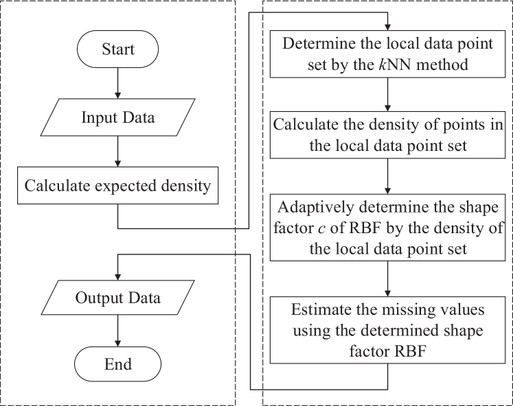
Figure 1: Flowchart of the adaptive RBF interpolation algorithm

2.2 Evaluating the Performance of Adaptive RBF Interpolation

In order to evaluate the computational accuracy of the adaptive RBF interpolation algorithm, we use the metric, Root Mean Square Error (RMSE) to measure the accuracy. The RMSE evaluates the error accuracy by comparing the deviation between the estimated value and the true value. Then, we compare the accuracy and efficiency of adaptive RBF estimator with the results of $k$NN and AIDW estimators.

3 Experimental Design

To evaluate the performance of the presented adaptive RBF interpolation algorithm we use three datasets to test it. The details of the experimental environment are listed in Table 1.

In our experiments, we use three datasets from three cities’ digital elevation model (DEM) (Fig.2(a) to Fig.2(c)), the range of three DEM maps is the same We randomly select 10% observed samples from each dataset as the samples with missing values, and the rest as the samples with known values. It should be noted that the samples with missing values have really elevation values in fact, but for testing, we assume the elevations are missing. Basic information of the datasets is listed in Table 2.

Table 1: Details of experimental environment

Specification	Details
OS	Windows 7. Professional
CPU	Intel (R) i5-4210U
CPU Frequency	1.70 GHz
CPU RAM	8 GB
CPU Core	4

Table 2: Details of the testing data

Dataset	Number of known values	Number of missing values	Illustration
Beijing	1,111,369	123,592	Fig.2(a)
Chongqing	1,074,379	97,525	Fig.2(b)
Longyan	1,040,670	119,050	Fig.2(c)

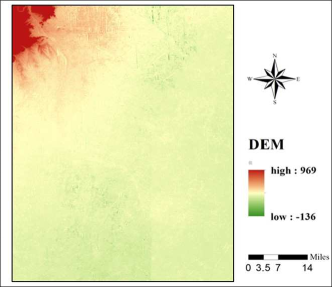
(a) DEM map of Beijing City

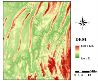
(b) DEM map of Chongqing City

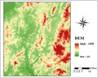
(c) DEM map of Longyan City

Figure 2: The DEM maps of three cities for the experimental tests.

4 Results and Discussion

We compare the accuracy and efficiency of adaptive RBF estimator with that of $k$NN and AIDW estimators.

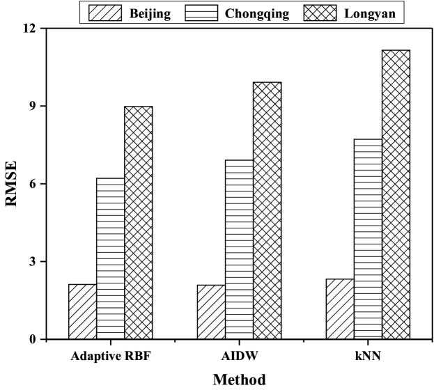
Figure 3: Comparisons of the computational accuracy

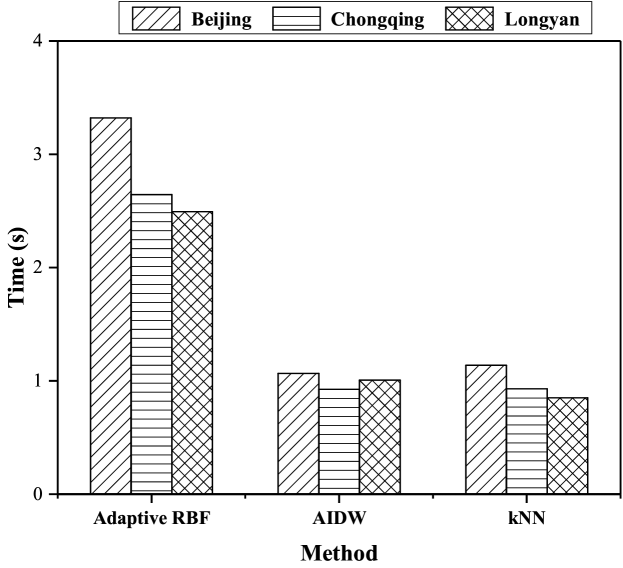
Figure 4: Comparisons of the computational efficiency

In Fig.3 and Fig.4, we find that the accuracy of the adaptive RBF estimator is the best performing, and the$k$NN estimator with the lowest accuracy. With the number of known data points in the datasets decreases, the accuracy of three estimators decreases significantly. Moreover, the computational efficiency of adaptive RBF estimator is worse than that of $k$NN estimator and AIDW estimator, among them,$k$NN has the best computational efficiency. With the increase of data quantity, the disadvantage of the computational efficiency of $k$NN estimator becomes more and more obvious.

The data points selected from DEM are evenly distributed, and the shape factor $c$ of the adaptive RBF interpolation algorithm is adapted according to the density of the points in the local dataset therefore, when the missing data is estimated in a dataset with a more uniform data point, the advantages of the adaptive RBF interpolation algorithm may not be realized. We need to do further research in datasets with uneven datasets

5 Conclusions

In this paper, we specifically proposed an adaptive RBF interpolation algorithm for estimating the missing values in geographical data. We performed three groups of experimental tests to evaluate the computational accuracy and efficiency of the proposed adaptive RBF interpolation by comparing with the $k$NN interpolation and AIDW method. We found that the accuracy of the adaptive RBF interpolation performs better than $k$NN interpolation and AIDW in regularly distributed datasets. But the efficiency of adaptive RBF interpolation is worse than the $k$NN interpolation and AIDW.

Acknowledgments

This research was jointly supported by the National Natural Science Foundation of China (11602235), and the Fundamental Research Funds for China Central Universities (2652018091, 2652018107, and 2652018109).

References

- [1] Barone, G.B., Boccia, V., Bottalico, D., Campagna, R., Carracciuolo, L., Laccetti, G., Lapegna, M.: An approach to forecast queue time in adaptive scheduling: How to mediate system efficiency and users satisfaction. International Journal of Parallel Programming 45(5), 1–30 (2016)
- [2] Cuomo, S., Galletti, A., Giunta, G., Marcellino, L.: Reconstruction of implicit curves and surfaces via rbf interpolation. Applied Numerical Mathematics 116, 60–63 (2016)
- [3] Cuomo, S., Gallettiy, A., Giuntay, G., Staracey, A.: Surface reconstruction from scattered point via rbf interpolation on gpu (2013)
- [4] Ding, Z., Mei, G., Cuomo, S., Tian, H., Xu, N.: Accelerating multi-dimensional interpolation using moving least-squares on the gpu. Concurrency Computation 30(24) (2018)
- [5] Ding, Z., Gang, M., Cuomo, S., Li, Y., Xu, N.: Comparison of estimating missing values in iot time series data using different interpolation algorithms. International Journal of Parallel Programming pp. 1–15 (2018)
- [6] Ding, Z., Gang, M., Cuomo, S., Xu, N., Hong, T.: Performance evaluation of gpu-accelerated spatial interpolation using radial basis functions for building explicit surfaces. International Journal of Parallel Programming (157), 1–29 (2017)
- [7] Gao, D., Liu, Y., Meng, J., Jia, Y., Fan, C.: Estimating significant wave height from sar imagery based on an svm regression model. Acta Oceanologica Sinica 37(3), 103–110 (2018)
- [8] Kedward, L., Allen, C.B., Rendall, T.C.S.: Efficient and exact mesh deformation using multiscale rbf interpolation. Journal of Computational Physics 345, 732–751 (2017)
- [9] Keogh, R.H., Seaman, S.R., Bartlett, J.W., Wood, A.M.: Multiple imputation of missing data in nested case-control and case-cohort studies. Biometrics 74(4) (2018)
- [10] Liang, Z., Na, Z., Wei, H., Feng, Z., Qiao, Q., Luo, M.: From big data to big analysis: a perspective of geographical conditions monitoring pp. 1–15
- [11] Lu, G.Y., Wong, D.W.: An adaptive inverse-distance weighting spatial interpolation technique. Computers & Geosciences 34(9), 1044–1055 (2008)
- [12] Mei, G., Xu, N., Xu, L.: Improving gpu-accelerated adaptive idw interpolation algorithm using fast knn search. Springerplus 5(1), 1389 (2016)
- [13] Skala, V.: Rbf interpolation with csrbf of large data sets. Procedia Computer Science 108, 2433–2437 (2017)
- [14] Sovilj, D., Eirola, E., Miche, Y., Björk, K.M., Rui, N., Akusok, A., Lendasse, A.: Extreme learning machine for missing data using multiple imputations. Neurocomputing 174(PA), 220–231 (2016)
- [15] Tang, T., Chen, S., Meng, Z., Wei, H., Luo, J.: Very large-scale data classification based on k-means clustering and multi-kernel svm. Soft Computing (1), 1–9 (2018)
- [16] Thakuriah, P., Tilahun, N.Y., Zellner, M.: Big data and urban informatics: Innovations and challenges to urban planning and knowledge discovery (2016)
- [17] Tomita, H., Fujisawa, H., Henmi, M.: A bias-corrected estimator in multiple imputation for missing data. Statistics in Medicine 47(1), 1–16 (2018)