Improved Coupling of Hydrodynamics and Nuclear Reactions via Spectral Deferred Corrections

Abstract

Simulations in stellar astrophysics involve the coupling of hydrodynamics and nuclear reactions under a wide variety of conditions, from simmering convective flows to explosive nucleosynthesis. Numerical techniques such as operator splitting (most notably Strang splitting) are usually employed to couple the physical processes, but this can affect the accuracy of the simulation, particularly when the burning is vigorous. Furthermore, Strang splitting does not have a straightforward extension to higher-order integration in time. We present a new temporal integration strategy based on spectral deferred corrections and describe the second- and fourth-order implementations in the open-source, finite-volume, compressible hydrodynamics code Castro. One notable advantage to these schemes is that they combine standard low-order discretizations for individual physical processes in a way that achieves an arbitrarily high order of accuracy. We demonstrate the improved accuracy of the new methods on several test problems of increasing complexity.

1 Introduction

Stellar astrophysical flows involve the delicate coupling of hydrodynamics, reactions, and other physics (gravity, radiation, magnetic fields, etc.). Whether modeling convective or explosive burning, reacting flows present temporal challenges to traditional algorithms used in stellar / nuclear astrophysics. Reaction network ODE systems are often stiff, containing timescales that are much smaller than hydrodynamic timescales. For this reason, astrophysical hydrodynamics codes often employ operator splitting to couple the reactions and hydrodynamics, treating the reactive portion of the evolution implicitly and the hydrodynamics explicitly, and allowing each to take their preferred internal timesteps. Strang-splitting (Strang, 1968) is a widely used technique for coupling in astrophysical systems (e.g., used in Castro, Almgren et al. 2010, Maestro, Nonaka et al. 2010, Flash, Fryxell et al. 2000, Chimera, Bruenn et al. 2018, PROMPI, Meakin & Arnett 2007, and many others), but it can break down in regions where energy is released faster than the hydrodynamics can respond. Traditional Strang splitting is also limited to second-order accuracy in time, although higher-order variants are possible.

As astrophysical hydrodynamics codes push to higher-order spatial accuracy (see, e.g., Wongwathanarat et al. 2016; Felker & Stone 2018; Most et al. 2019), new time-integration schemes are needed to realize the potential of high-order methods. Here we look at alternate ways to couple hydrodynamics and reactions, in particular, spectral deferred correction (SDC) methods. We describe a fully fourth-order method in space and time for coupling hydrodynamics and reactions in the open source, finite-volume, compressible Castro code. One notable advantage of SDC schemes is that they combine standard low-order discretizations for individual physical processes in a way that achieves an arbitrarily high order of accuracy. Here we evaluate these methods on a suite of test problems with the ultimate goal of modeling thermonuclear flame propagation in X-ray bursts, as we described in Zingale et al. (2019). In X-ray bursts, the range of lengthscales and tight hydrostatic equilibrium of the atmosphere make models that capture the burning, flame scale, and global scales of the neutron star challenging. This problem is an ideal candidate for higher-order methods.

The presentation in this paper is described as follows. In § 2 we describe the model equations of interest. In § 3 we present an overview of the Strang splitting methods and the second- and fourth-order SDC approaches. In § 4 we present the complete details of our SDC approach. In § 5 we demonstrate the accuracy of the new schemes on several different test problems, and in § 6 we discuss the strengths and weaknesses of the new scheme and future plans for extending the methods for more complex equations of interest.

2 Model Equations

The governing equations of interest in this work are based on the fully compressible Euler equations, including thermal diffusion. Since our focus is on time-integration, we restrict the presentation to 1- and 2-d problems in this paper, but the method is straightforward to extend to 3-d. In conservation-law form, the 2-d system can be written

$${\,\bm{\mathcal{U}}}_{t}+[\mathbf{F}^{(x)}({\,\bm{\mathcal{U}}})]_{x}+[\mathbf{F}^{(y)}({\,\bm{\mathcal{U}}})]_{y}=\mathbf{S}({\,\bm{\mathcal{U}}}),$$ (1)

where ${\,\bm{\mathcal{U}}}=(\rho,(\rho X_{k}),(\rho\mathbf{U}),(\rho E),(\rho e))^{\intercal}$ is the vector of conserved quantities, $\mathbf{F}^{(x)}$ and $\mathbf{F}^{(y)}$ are the fluxes in the $x$- and $y$-directions, and $\mathbf{S}$ are source terms. Here, $\rho$ is the mass density, $\mathbf{U}$ is the velocity vector with components $u$ and $v$, $E$ is the specific total energy, related to the specific internal energy, $e$, as

$$E=e+|\mathbf{U}|^{2}/2$$ (2)

and $X_{k}$ are the mass fractions of the reacting species, constrained such that $\sum_{k}X_{k}=1$. The use of both $E$ and $e$ is overdetermined; this is done for cases where calculating $e$ via $E-|\mathbf{U}|^{2}/2$ yields an unreliable internal energy. One example is roundoff error in regions of high Mach number flows (Bryan et al., 1995). The general stellar equation of state we use here, with weak temperature-dependency in $e$ for highly-degenerate gases also benefits from the dual-energy approach. The use of both $\rho X$ and $\rho$ is also overdetermined, however we integrate both to numerically ensure that we conserve total mass.

The fluxes are

$$\mathbf{F}^{(x)}({\,\bm{\mathcal{U}}})=\left(\begin{array}[]{c}\rho u\\ \rho X_{k}u\\ \rho uu+p\\ \rho vu\\ \rho uE+up\\ \rho ue\end{array}\right)\,,\quad\mathbf{F}^{(y)}({\,\bm{\mathcal{U}}})=\left(\begin{array}[]{c}\rho v\\ \rho X_{k}v\\ \rho uv\\ \rho vv+p\\ \rho vE+vp\\ \rho ve\end{array}\right)\,,\quad$$ (3)

Here the pressure, $p$, enters, and is found via the equation of state,

$$p=p(\rho,X_{k},e)$$ (4)

Finally, the source terms for our system typically include gravity, thermal diffusion, and reactive terms. For computational efficiency, it is advantageous to treat the reactive terms separately from the other hydrodynamics source terms, so we split this into two components, ${{\bf H}}$, the hydrodynamic source, and ${\bf R}$, the reactive source. We note that since the $(\rho e)$ equation is not conservative, we include the “$pdV$” work term, $p\nabla\cdot\mathbf{U}$, as a source term for that component.

$$\mathbf{S}({\,\bm{\mathcal{U}}})=\left(\begin{array}[]{c}0\\ \rho\dot{\omega}_{k}\\ \rho\mathbf{g}\cdot{\bf e}_{x}\\ \rho\mathbf{g}\cdot{\bf e}_{y}\\ \rho\mathbf{U}\cdot\mathbf{g}+\rho\dot{S}+\nabla\cdot k_{\mathrm{th}}\nabla T\\ -p\nabla\cdot\mathbf{U}+\rho\dot{S}+\nabla\cdot k_{\mathrm{th}}\nabla T\end{array}\right)=\underbrace{\left(\begin{array}[]{c}0\\ 0\\ \rho\mathbf{g}\cdot{\bf e}_{x}\\ \rho\mathbf{g}\cdot{\bf e}_{y}\\ \rho\mathbf{U}\cdot\mathbf{g}+\nabla\cdot k_{\mathrm{th}}\nabla T\\ -p\nabla\cdot\mathbf{U}+\nabla\cdot k_{\mathrm{th}}\nabla T\end{array}\right)}_{{{\bf H}}({\,\bm{\mathcal{U}}})}+\underbrace{\left(\begin{array}[]{c}0\\ \rho\dot{\omega}_{k}\\ 0\\ 0\\ \rho\dot{S}\\ \rho\dot{S}\end{array}\right)}_{{\bf R}\left({\,\bm{\mathcal{U}}}\right)}$$ (5)

Here, the species are characterized by mass fractions, $X_{k}$, and change via their creation rates, $\dot{\omega}_{k}$, and the energy has a corresponding specific energy generation rate, $\dot{S}$. The gravitational acceleration, $\mathbf{g}$, is found either by solving the Poisson equation,

$$\nabla^{2}\Phi=4\pi G\rho$$ (6)

for the potential, $\Phi$, and then $\mathbf{g}=-{\mathbf{\nabla}}\Phi$, or by externally specifying $\mathbf{g}$, with the Cartesian unit vectors denoted ${\bf e}_{x}$ and ${\bf e}_{y}$. For the present work, we consider only constant gravity (appropriate for our target XRB problem). Since the reactions and diffusion term depend on temperature, to close the system of equations our equation of state also needs to return temperature, $T$,

$$T=T(\rho,X_{k},e)$$ (7)

The thermal conductivity, $k_{\mathrm{th}}$, is likewise a function of the thermodynamic state:

$$k_{\mathrm{th}}=k_{\mathrm{th}}(\rho,X_{k},T)$$ (8)

We note that the thermal diffusion term could instead be included in the definition of the fluxes, since it is represented as the divergence of the diffusive flux. We use this later in the construction of a fourth-order approximation to thermal diffusion.

We rewrite our system as:

$${\,\bm{\mathcal{U}}}_{t}=\bm{\mathcal{A}}\left({\,\bm{\mathcal{U}}}\right)+{\bf R}\left({\,\bm{\mathcal{U}}}\right)$$ (9)

where we define the advective term, $\bm{\mathcal{A}}\left({\,\bm{\mathcal{U}}}\right)$ to include the hydrodynamic source terms:

$$\bm{\mathcal{A}}\left({\,\bm{\mathcal{U}}}\right)\equiv-[\mathbf{F}^{(x)}({\,\bm{\mathcal{U}}})]_{x}-[\mathbf{F}^{(y)}({\,\bm{\mathcal{U}}})]_{y}+{{\bf H}}({\,\bm{\mathcal{U}}})$$ (10)

We denote the discretized advective source with a cell subscript, as ${\left[\bm{\mathcal{A}}\left({\,\bm{\mathcal{U}}}\right)\right]}_{i,j}$.

3 Algorithmic Overview

3.1 Strang Split Method

A Strang-split integration method (Strang, 1968) is an operator splitting technique that alternates reactions and hydrodynamics, with each indirectly seeing the effects of the other. No direct coupling is provided, but by staggering the operations, second-order accuracy is achieved. The basic algorithm to advance the solution over a time step $\delta t$ proceeds as:

• Integrate the reactive portion of the system through $\delta t/2$: We solve

  $$\frac{d{\,\bm{\mathcal{U}}}_{i,j}}{dt}={\bf R}\left({\,\bm{\mathcal{U}}}_{i,j}\right)$$ (11)

  starting with ${\,\bm{\mathcal{U}}}^{n}$, yielding the solution ${\,\bm{\mathcal{U}}}^{\star}$. This is actually an ODE system, so we can use any implicit ODE integration scheme for this. This evolution only sees the effects of reactions, not advection. The species portion of the system has the form:

  $$\frac{dX_{k}}{dt}=\dot{\omega}_{k}(\rho,T,X_{k})$$ (12)

  Accurate rate evaluation implies we need accurate temperature and density approximations, which suggests we should evolve the energy equation together with the species (Müller, 1986). We can cast this in terms of temperature,

  $$\rho c_{x}\frac{dT}{dt}=\rho\dot{S}$$ (13)

  where $c_{x}$ is the specific heat. This form is missing the “$pdV$” work term $p\nabla\cdot\mathbf{U}$, since we are splitting the advective portion out of the reactive system. For a constant volume burn, $c_{x}=c_{v}$ is usually taken, while for a constant pressure burn, $c_{x}=c_{p}$ is taken (see, e.g., Almgren et al. 2008). Again, if we were not splitting, then this choice would not matter, since the correct form of the work term would also appear. Both Eqs. 12 and 13 are also missing the advective terms as well, so the extent to which the flow can transport fuel in and out of a cell is not accounted for during the burn.

• Advance the advective part through $\delta t$: We solve

  $$\frac{\partial{\,\bm{\mathcal{U}}}_{i,j}}{\partial t}={\left[\bm{\mathcal{A}}\left({\,\bm{\mathcal{U}}}\right)\right]}_{i,j}$$ (14)

  integrating through the full $\delta t$, starting with ${\,\bm{\mathcal{U}}}^{\star}$ to get the state ${\,\bm{\mathcal{U}}}^{n+1,\star}$. No reaction sources are explicitly included, but since the first step integrated the effects of reactions to $\delta t/2$, the state that we build the advection from, ${\,\bm{\mathcal{U}}}^{\star}$, is already time-centered with the effects of reactions, allowing us to be second-order in time (see Strang 1968 for a more formal discussion).

• Integrate the second half of reactions, through $\delta t/2$: We again solve

  $$\frac{d{\,\bm{\mathcal{U}}}_{i,j}}{dt}={\bf R}\left({\,\bm{\mathcal{U}}}_{i,j}\right)$$ (15)

  starting with ${\,\bm{\mathcal{U}}}^{n+1,\star}$, yielding the final solution ${\,\bm{\mathcal{U}}}^{n+1}$.

With Strang splitting, there is no mechanism for the total density to evolve during reactions (since that evolves solely through the advective terms), so the burning is done at constant density. Additionally, for stellar material, the specific heat can be a strong function of temperature, so we should allow the specific heat to evolve with the other variables, which means augmenting the evolution of our system with an equation of state call to keep the specific heat consistent. This is sometimes neglected.

In Zingale et al. (2019), the authors examine the numerical representation of the solution over a time step for flow behind a detonation, comparing Strang splitting to a simplified-SDC method. This comparison shows that the Strang react-advect-react sequence has strong departures from equilibrium over the course of a step as compared to the simplified-SDC method. The latter approach leads to a smooth representation of the solution over a time step due to improved advection/reaction coupling. The consequence of Strang splitting is that the departure from equilibrium requires much more computational work in the reaction steps due to the stiff transients present as the system returns to equilibrium. For astrophysical reacting flow computations, the burning and EOS components can require more computational effort than the hydrodynamic components, so temporal methods that can reduce the number of right-hand side calls in the reaction steps by staying closer to equilibrium are advantageous.

We make one final note: the ODE system in the react step is done with a specified numerical tolerance. Tightening the tolerance means solving the reacting system more accurately, but since we are neglecting the hydrodynamics, we are in essence solving the wrong equations very accurately. So simply increasing the tolerances does not necessarily lead to a more accurate solution, nor does it help improve the coupling with hydrodynamics.

3.2 Method-of-Lines Integration

Instead of splitting, we could discretize the entire system in space and then use an ODE integrator to handle the time evolution, a technique called method-of-lines integration. This would give us an ordinary differential equations system to integrate of the form:

$$\frac{d{\,\bm{\mathcal{U}}}_{i,j}}{dt}={\left[\bm{\mathcal{A}}\left({\,\bm{\mathcal{U}}}\right)\right]}_{i,j}+{\bf R}\left({\,\bm{\mathcal{U}}}_{i,j}\right)$$ (16)

In an explicit MOL approach, both the advective and reactive terms are evaluated with the same state in constructing the right-hand side. The difficulty here arises if the reaction sources are stiff. We need to use the same timestep for both the reactions and hydrodynamics, and if we want to treat the system explicitly (as we would like for hydrodynamics), then we are constrained to evolve the entire system at the restrictive timestep dictated by the reactions. This can be computationally infeasible. Implicit and semi-implicit MOL approaches (e.g., IMEX/Runge-Kutta approaches) suffer from other maladies including the need to solve expensive coupled nonlinear equations, difficulty in generalizing to very high orders of accuracy, and difficulty in adding additional physical processes (Dutt et al., 2000; Minion, 2003). With these limitations in mind, here we explore the SDC approach.

3.3 General SDC Algorithm

Generally, SDC algorithms are a class of numerical methods that represent the solution as an integral in time and iteratively solve a series of correction equations designed to reduce both the integration and splitting error. The correction equations are typically formed using a low-order time-integration scheme (e.g., forward or backward Euler), but are applied iteratively to construct schemes of arbitrarily high accuracy. In practice, the time step is divided into a series of sub steps separated by nodes, and the solution at these nodes is iteratively improved by utilizing high-order integral representations of the solution from the previous iteration as a source term in the temporal integration.

The original SDC approach was introduced by Dutt et al. (2000) for ODEs where the integration of the ODE, as well as the associated correction equations, is performed using forward or backward Euler discretizations. Minion (2003) introduced a semi-implicit version (SISDC) for ODEs with stiff and non-stiff processes. The correction equations for the non-stiff terms are discretized explicitly, whereas the stiff term corrections are treated implicitly. While these works describe the solution of ODEs, they can be applied to PDEs discretizing in space and applying the method of lines. Others have adapted this approach for multiphysics PDE simulation in a variety of contexts (3 time scales with substepping; finite volume/finite difference; compressible/incompressible and/or low Mach number reacting flow) to very high orders of accuracy (up to eighth-order); see Bourlioux et al. (2003); Almgren et al. (2013); Emmett et al. (2014); Pazner et al. (2016); Emmett et al. (2019). Here we leverage these ideas to develop a finite-volume, fourth-order spatio-temporal integrator for compressible astrophysical flow that couples reactions and hydrodynamics in a semi-implicit manner.

The basic idea of SDC is to write the solution of a system of ODEs

$$\frac{d{\,\bm{\mathcal{U}}}}{dt}=\mathbf{f}(t,{\,\bm{\mathcal{U}}}(t)),\quad t\in[t^{n},t^{n}+\delta t],\quad{\,\bm{\mathcal{U}}}(t^{n})\equiv{\,\bm{\mathcal{U}}}^{n},$$ (17)

in the equivalent Picard integral form,

$${\,\bm{\mathcal{U}}}(t)={\,\bm{\mathcal{U}}}^{n}+\int_{t^{n}}^{t}\mathbf{f}({\,\bm{\mathcal{U}}})d\tau,$$ (18)

where we suppress explicit dependence of $\mathbf{f}$ and ${\,\bm{\mathcal{U}}}$ on $t$ for notational simplicity. Given an approximation ${\,\bm{\mathcal{U}}}^{(k)}(t)$ to ${\,\bm{\mathcal{U}}}(t)$, the SDC correction equation is constructed by discretizing

$${\,\bm{\mathcal{U}}}^{(k+1)}(t)={\,\bm{\mathcal{U}}}^{n}+\int_{t^{n}}^{t}\left[\mathbf{f}({\,\bm{\mathcal{U}}}^{(k+1)})-\mathbf{f}({\,\bm{\mathcal{U}}}^{(k)})\right]d\tau+\int_{t^{n}}^{t}\mathbf{f}({\,\bm{\mathcal{U}}}^{(k)})d\tau,$$ (19)

where a low-order discretization (e.g., forward or backward Euler) is used for the first integral and a higher-order quadrature is used to evaluate the second integral. Each iteration improves the overall order of accuracy of the approximation by one per iteration, up to the order of accuracy of the underlying quadrature rule used to evaluate the second integral.

For a given time step, we begin with a state at time $t^{n}$ and seek to updated it through $\delta t$ to time $t^{n+1}$. For the SDC method, we divide this time interval into ${M}$ subintervals using ${M}+1$ temporal nodes, $t^{0}<t^{1}<\cdots<t^{{M}}$. For the cases presented here, one time node is at the beginning of the full time step ($t^{0}\equiv t^{n}$) and one of at the end of the full time step $t^{M}\equiv t^{n+1}$. For a fourth-order approach, we can use 3-point Gauss-Lobatto quadrature with nodes located at the beginning, midpoint, and end of the time step. Using the notation ${\,\bm{\mathcal{U}}}^{m,(k)}$ to denote the $k^{\rm th}$ iterate of the solution at node $m$, we can generalize (19) to update the solution at a particular node

$${\,\bm{\mathcal{U}}}^{m+1,(k+1)}={\,\bm{\mathcal{U}}}^{m,(k+1)}+\int_{t^{m}}^{t^{m+1}}\left[\mathbf{f}({\,\bm{\mathcal{U}}}^{(k+1)})-\mathbf{f}({\,\bm{\mathcal{U}}}^{(k)})\right]d\tau+\int_{t^{m}}^{t^{m+1}}\mathbf{f}({\,\bm{\mathcal{U}}}^{(k)})d\tau$$ (20)

Thus, a pure forward-Euler discretization of the first integral results in the update,

$${\,\bm{\mathcal{U}}}^{m+1,(k+1)}={\,\bm{\mathcal{U}}}^{m,(k+1)}+\delta t_{m}\left[\mathbf{f}({\,\bm{\mathcal{U}}}^{m,(k+1)})-\mathbf{f}({\,\bm{\mathcal{U}}}^{m,(k)})\right]+\int_{t^{m}}^{t^{m+1}}\mathbf{f}({\,\bm{\mathcal{U}}}^{(k)})d\tau$$ (21)

Note that overall this is an explicit computation of ${\,\bm{\mathcal{U}}}^{m+1,(k+1)}$ since all the terms on the right-hand side are available via explicit computation .

Our model contains advection and reaction terms,

$${\,\bm{\mathcal{U}}}^{n+1}={\,\bm{\mathcal{U}}}^{n}+\int(\bm{\mathcal{A}}\left({\,\bm{\mathcal{U}}}\right)+{\bf R}\left({\,\bm{\mathcal{U}}}\right))dt$$ (22)

Stiff terms (e.g. reactions) can be treated implicitly while non-stiff terms (e.g. the hydrodynamics) can be treated explicitly. Following Minion (2003), the correction equation contains an explicit and implicit part:

$${\,\bm{\mathcal{U}}}^{m+1,(k+1)}={\,\bm{\mathcal{U}}}^{m,(k+1)} + \delta t_{m}\left[\bm{\mathcal{A}}\left({\,\bm{\mathcal{U}}}^{m,(k+1)}\right)-\bm{\mathcal{A}}\left({\,\bm{\mathcal{U}}}^{m,(k)}\right)\right]+$$ (23)

$$+ \delta t_{m}\left[{\bf R}\left({\,\bm{\mathcal{U}}}^{m+1,(k+1)}\right)-{\bf R}\left({\,\bm{\mathcal{U}}}^{m+1,(k)}\right)\right]$$

$$+ \int_{t^{m}}^{t^{m+1}}\bm{\mathcal{A}}\left({\,\bm{\mathcal{U}}}^{(k)}\right)+{\bf R}\left({\,\bm{\mathcal{U}}}^{(k)}\right)d\tau.$$

Now we note that overall this is an implicit equation for reactions solving for ${\,\bm{\mathcal{U}}}^{m+1,(k+1)}$; all terms on the right-hand side except for ${\bf R}({\,\bm{\mathcal{U}}}^{m+1,(k+1)})$ are available via explicit computation. Thus, the update at each node amounts to solving an implicit reaction equation with explicitly computed source terms from advection, as well as previously computed reaction terms.

4 Algorithmic Details

Here we describe the fourth-order algorithm in full detail. For proper construction of fourth-order methods, we need to distinguish between cell-average values and cell-center values (i.e., point values) in the finite-volume framework. We use angled braces, e.g. ${\left\langle{\,\bm{\mathcal{U}}}\right\rangle}_{i,j}$, to denote a cell average and ${\,\bm{\mathcal{U}}}_{i,j}$ to denote a cell-center value. For expressions involving the time-update for a single zone, we will drop the spatial subscripts, ${i,j}$. In the SDC equations, we denote the state with two time superscripts, ${\left\langle{\,\bm{\mathcal{U}}}\right\rangle}^{m,(k)}$, where $m$ represents the quadrature point in the time-discretization and $k$ represents the iteration number. A general SDC update for our state ${\left\langle{\,\bm{\mathcal{U}}}\right\rangle}$ takes the form:

• For all SDC iterations $k\in[0,{K}-1]$, we initialize the state, advective update, and reaction source for $m=0$ equal to the state at $t^{n}$ (i.e., the state at the $m=0$ node doesn’t change with iteration and is equal to the state at $t^{n})$;

  $${\left\langle{\,\bm{\mathcal{U}}}\right\rangle}^{0,(k)} ={\left\langle{\,\bm{\mathcal{U}}}\right\rangle}^{n}$$ (24)

  $${\left\langle\bm{\mathcal{A}}\left({\,\bm{\mathcal{U}}}\right)\right\rangle}^{0,(k)} ={\left\langle\bm{\mathcal{A}}\left({\,\bm{\mathcal{U}}}\right)\right\rangle}^{n}$$ (25)

  $${\left\langle{\bf R}\left({\,\bm{\mathcal{U}}}\right)\right\rangle}^{0,(k)} ={\left\langle{\bf R}\left({\,\bm{\mathcal{U}}}\right)\right\rangle}^{n}$$ (26)

• We need values of $\bm{\mathcal{A}}\left({\,\bm{\mathcal{U}}}\right)$ and ${\bf R}({\,\bm{\mathcal{U}}})$ at all time nodes to do the integral over the iteratively-lagged state in the first iteration. For all temporal nodes $m\in[1,{M}]$, we initialize the state, advective update, and reaction source for $k=0$ equal to the state at $t^{n}$ (i.e., copy the $t^{n}$ state into each temporal node to initialize the time step).

  $${\left\langle{\,\bm{\mathcal{U}}}\right\rangle}^{m,(0)} ={\left\langle{\,\bm{\mathcal{U}}}\right\rangle}^{n}$$ (27)

  $${\left\langle\bm{\mathcal{A}}\left({\,\bm{\mathcal{U}}}\right)\right\rangle}^{m,(0)} ={\left\langle\bm{\mathcal{A}}\left({\,\bm{\mathcal{U}}}\right)\right\rangle}^{n}$$ (28)

  $${\left\langle{\bf R}\left({\,\bm{\mathcal{U}}}\right)\right\rangle}^{m,(0)} ={\left\langle{\bf R}\left({\,\bm{\mathcal{U}}}\right)\right\rangle}^{n}$$ (29)

• Loop from $k=0,\ldots,{K}-1$

  This is the main iteration loop, and each pass results in an improved value of ${\left\langle{\,\bm{\mathcal{U}}}\right\rangle}$ at each of the time nodes.

  • Loop over time nodes, from $m=0,\ldots,{M}-1$

    • Compute ${\left\langle\bm{\mathcal{A}}\left({\,\bm{\mathcal{U}}}\right)\right\rangle}^{m,(k)}$ from ${\,\bm{\mathcal{U}}}^{m,(k)}$

    • Solve:

      $${\left\langle{\,\bm{\mathcal{U}}}\right\rangle}^{{m+1},(k+1)}={\left\langle{\,\bm{\mathcal{U}}}\right\rangle}^{m,(k+1)} +\delta t_{m}\left[{\left\langle\bm{\mathcal{A}}\left({\,\bm{\mathcal{U}}}\right)\right\rangle}^{m,(k+1)}-{\left\langle\bm{\mathcal{A}}\left({\,\bm{\mathcal{U}}}\right)\right\rangle}^{m,(k)}\right]$$

      $$+\delta t_{m}\left[{\left\langle{\bf R}\left({\,\bm{\mathcal{U}}}\right)\right\rangle}^{{m+1},(k+1)}-{\left\langle{\bf R}\left({\,\bm{\mathcal{U}}}\right)\right\rangle}^{{m+1},(k)}\right]$$

      $$+\bm{\mathcal{I}}_{m}^{m+1}\left({\left\langle\bm{\mathcal{A}}\left({\,\bm{\mathcal{U}}}\right)\right\rangle}^{(k)}+{\left\langle{\bf R}\left({\,\bm{\mathcal{U}}}\right)\right\rangle}^{(k)}\right)$$ (30)

      where $\delta t_{m}=t^{m+1}-t^{m}$. The last term is an integral:

      $$\bm{\mathcal{I}}_{m}^{m+1}\left({\left\langle\bm{\mathcal{A}}\left({\,\bm{\mathcal{U}}}\right)\right\rangle}^{(k)}+{\left\langle{\bf R}\left({\,\bm{\mathcal{U}}}\right)\right\rangle}^{(k)}\right) \approx$$

      $$\int_{t^{m}}^{t^{m+1}}dt \left({\left\langle\bm{\mathcal{A}}\left({\,\bm{\mathcal{U}}}\right)\right\rangle}^{(k)}+{\left\langle{\bf R}\left({\,\bm{\mathcal{U}}}\right)\right\rangle}^{(k)}\right)$$ (31)

      which we evaluate using an appropriate numerical quadrature rule with our ${M}+1$ integration points, using the right hand side values from the previous iteration.

We note that Eq. * ‣ – ‣ • ‣ 4 is an implicit nonlinear equation for ${\left\langle{\,\bm{\mathcal{U}}}\right\rangle}^{m+1,(k+1)}$. There are four terms on the right-hand side. The second term is the increment in advection from one SDC iteration to the next, written as a forward Euler (explicit) update to the solution from one time quadrature point to the next. The third term (the increment in the reaction term) appears as a backwards Euler (implicit) update to the solution. Note the reaction terms here are the instantaneous rates—there is no ODE integration. If the SDC iterations converge, then the increment in advection and reactions (the second and third terms) go to zero, and the SDC substeps tend toward:

$${\left\langle{\,\bm{\mathcal{U}}}\right\rangle}^{{m+1},(k+1)}\approx{\left\langle{\,\bm{\mathcal{U}}}\right\rangle}^{m,(k+1)}+\int_{t^{m}}^{t^{m+1}}\mathrm{d}t\left({\left\langle\bm{\mathcal{A}}\left({\,\bm{\mathcal{U}}}\right)\right\rangle}^{(k)}+{\left\langle{\bf R}\left({\,\bm{\mathcal{U}}}\right)\right\rangle}^{(k)}\right).$$ (32)

Hence the SDC solution converges to that of a fully implicit Gauss-Runge-Kutta (also referred to as collocation) method (Huang et al., 2006). This implies that the integrals that span the full timestep ultimately determine the accuracy of the method, and we pick the number of quadrature nodes $M+1$, to yield the desired time accuracy over the timestep. Lobatto methods have formal order $2M$, hence we use 2 nodes for second-order in time, and 3 nodes for fourth-order in time. We also see that during the SDC substeps for each process (advection and reacting), terms coupling other processes are included, giving us the strong coupling we desire.

Finding the new value of ${\left\langle{\,\bm{\mathcal{U}}}\right\rangle}$ requires a nonlinear solve of

$${\left\langle{\,\bm{\mathcal{U}}}\right\rangle}^{m+1,(k+1)}-\delta t_{m}{\left\langle{\bf R}\left({\,\bm{\mathcal{U}}}\right)\right\rangle}^{m+1,(k+1)}={\left\langle{\,\bm{\mathcal{U}}}\right\rangle}^{m,(k+1)}+\delta t_{m}{\left\langle\bf C\right\rangle}$$ (33)

where the right-hand side is constructed only from known states, and we define ${\left\langle\bf C\right\rangle}$ for convenience as:

$${\left\langle\bf C\right\rangle} =\left[{\left\langle\bm{\mathcal{A}}\left({\,\bm{\mathcal{U}}}\right)\right\rangle}^{m,(k+1)}-{\left\langle\bm{\mathcal{A}}\left({\,\bm{\mathcal{U}}}\right)\right\rangle}^{m,(k)}\right]-{\left\langle{\bf R}\left({\,\bm{\mathcal{U}}}\right)\right\rangle}^{{m+1},(k)}$$

$$+\frac{1}{\delta t_{m}}\bm{\mathcal{I}}_{m}^{m+1}\left({\left\langle\bm{\mathcal{A}}\left({\,\bm{\mathcal{U}}}\right)\right\rangle}^{(k)}+{\left\langle{\bf R}\left({\,\bm{\mathcal{U}}}\right)\right\rangle}^{(k)}\right)$$ (34)

and note that it represents an average over the cell.

4.1 Second-order Algorithm

For second-order, we need only 2 quadrature points (M = 1), $m=0$ corresponding to the old time solution, and $m=1$ corresponding to the new time solution. In this case, the second term in Eq. * ‣ – ‣ • ‣ 4 (the increment in advection terms from one iteration to the next) cancels, since regardless of the iteration, $k$, the solution at the old time ($m=0$) is the same. We can approximate our integral using the trapezoid rule, which is second-order accurate. We drop the $m$ superscript in what follows and simply denote the solution as either at time-level $n$ or $n+1$. Finally, to second-order accuracy in space, we can take the cell-averages to be cell-centers, and write ${\left\langle{\,\bm{\mathcal{U}}}\right\rangle}_{i,j}={\,\bm{\mathcal{U}}}_{i,j}$. The overall integration is then:

• Loop from $k=0,\ldots,{K}-1$

  • Solve:

    $${\,\bm{\mathcal{U}}}^{n+1,(k+1)}={\,\bm{\mathcal{U}}}^{n} +\delta t\left[{\bf R}\left({\,\bm{\mathcal{U}}}^{n+1,(k+1)}\right)-{\bf R}\left({\,\bm{\mathcal{U}}}^{n+1,(k)}\right)\right]$$

    $$+\frac{\delta t}{2}\left[\bm{\mathcal{A}}\left({\,\bm{\mathcal{U}}}^{n}\right)+\bm{\mathcal{A}}\left({\,\bm{\mathcal{U}}}^{n+1,(k)}\right)+{\bf R}\left({\,\bm{\mathcal{U}}}^{n}\right)+{\bf R}\left({\,\bm{\mathcal{U}}}^{n+1,(k)}\right)\right]$$ (35)

    We note that this is an implicit nonlinear equation for ${\,\bm{\mathcal{U}}}^{n+1,(k+1)}$.

  • Using this ${\,\bm{\mathcal{U}}}^{n+1,(k+1)}$, compute $\bm{\mathcal{A}}({\,\bm{\mathcal{U}}}^{n+1,(k+1)})$ and ${\bf R}({\,\bm{\mathcal{U}}}^{n+1,(k+1)})$ for use in the next iteration.

Choosing ${K}=2$ is sufficient for second-order accuracy.

To construct the advective term, $\bm{\mathcal{A}}\left({\,\bm{\mathcal{U}}}\right)$, we use piecewise linear reconstruction with the slope limiter from Colella (1985). The reconstructed slopes give us the edge states for each interface and we solve the Riemann problem to get the fluxes through the interface state.

To solve the update to second-order, we can ignore the difference between cell centers and cell-averages, and simply solve an implicit equation of the form:

$${\bf Z}({\,\bm{\mathcal{U}}}^{n+1})={\,\bm{\mathcal{U}}}^{n+1}-\delta t_{m}{\bf R}\left({\,\bm{\mathcal{U}}}^{n+1}\right)-{\,\bm{\mathcal{U}}}^{n}-\delta t_{m}{\bf C}=0$$ (36)

(we drop the iteration index, $k$, on the unknown here, and use the old and new time levels, $n$ and $n+1$ since there are no intermediate time nodes). This allows the update of a cell to be independent of other cells.

4.1.1 Solving the nonlinear system

We use a simple Newton iteration to solve Eq. 36. As we discuss below, an accurate initial guess may be required for the iteration to converge, especially for complex or very stiff networks. Given an initial guess for the solution, ${\,\bm{\mathcal{U}}}_{0}$, we seek a correction, $\delta{\,\bm{\mathcal{U}}}$, as

$${\bf Z}({\,\bm{\mathcal{U}}}_{0}+\delta{\,\bm{\mathcal{U}}})={\bf Z}({\,\bm{\mathcal{U}}}_{0})+{\bf J}\delta{\,\bm{\mathcal{U}}}+\ldots\approx 0$$ (37)

Here, J is the Jacobian, $\partial{\bf Z}/\partial{\,\bm{\mathcal{U}}}$. For the reactions, a more natural representation to work in is ${\bf w}=(\rho,X_{k},\mathbf{U},T)^{\intercal}$, as reaction networks typically provide a Jacobian in these terms. Our full Jacobian is then:

$${\bf J}\equiv\frac{\partial{\bf Z}}{\partial{\,\bm{\mathcal{U}}}}={\bf I}-\delta t_{m}\frac{\partial{\bf R}}{\partial{\,\bm{\mathcal{U}}}}={\bf I}-\delta t_{m}\frac{\partial{\bf R}}{\partial{\bf w}}\frac{\partial{\bf w}}{\partial{\,\bm{\mathcal{U}}}}$$ (38)

where we can compute $\partial{\bf w}/\partial{\,\bm{\mathcal{U}}}$ as $(\partial{\,\bm{\mathcal{U}}}/\partial{\bf w})^{-1}$, and the reaction network provides $\partial{\bf R}/\partial{\bf w}$.

Solving Eq. 37 requires solving the linear system ${\bf J}\delta{\,\bm{\mathcal{U}}}=-{\bf Z}({\,\bm{\mathcal{U}}}_{0})$. In practice, we only need to do the implicit solve for ${\,\bm{\mathcal{U}}}^{\prime}=(\rho,\rho X_{k},\rho e)^{\intercal}$ with ${\bf w}^{\prime}=(\rho,X_{k},T)^{\intercal}$, reducing the size of the Jacobian, and we can update the momentum, $\rho\mathbf{U}$, explicitly. We always compute $\partial{\bf w}/\partial{\,\bm{\mathcal{U}}}$ analytically, but $\partial{\bf R}/\partial{\bf w}$ is computed either numerically, via differencing, or analytically, depending on the reaction network. Appendix A gives the form of these matrices. We solve iteratively, applying the correction $\delta{\,\bm{\mathcal{U}}}$ to our guess ${\,\bm{\mathcal{U}}}_{0}$ until $\delta{\,\bm{\mathcal{U}}}$ satisfies

$$\left\{\frac{1}{N+2}\left[\left|\delta{\,\bm{\mathcal{U}}}(\rho)\,w_{\rho}\right|^{2}+\left|\delta{\,\bm{\mathcal{U}}}(\rho e)\,w_{(\rho e)}\right|^{2}+\sum_{k=1}^{N}\left|\delta{\,\bm{\mathcal{U}}}(\rho X_{k})\,w_{(\rho X_{k})}\right|^{2}\right]\right\}^{1/2}<1,$$ (39)

We specify separate relative tolerances for the density, species, and energy, ${\epsilon_{\mathrm{rel},\rho}}$, ${\epsilon_{\mathrm{rel},(\rho X)}}$, and ${\epsilon_{\mathrm{rel},(\rho e)}}$ respectively, as well as an overall absolute tolerance, ${\epsilon_{\mathrm{abs}}}$, and $N$ is the number of species in the network. We use a tolerance comparable to what we would use when integrating a reaction network directly. For each of the state components of ${\,\bm{\mathcal{U}}}$ we define a weight the form:

$$w_{\rho} =\left[{{\epsilon_{\mathrm{rel},\rho}}|{\,\bm{\mathcal{U}}}(\rho)|+{\epsilon_{\mathrm{abs}}}}\right]^{-1}\enskip,$$ (40)

$$w_{(\rho e)} =\left[{{\epsilon_{\mathrm{rel},(\rho e)}}|{\,\bm{\mathcal{U}}}(\rho e)|+{\epsilon_{\mathrm{abs}}}}\right]^{-1}\enskip,$$ (41)

$$w_{(\rho X_{k})} =\left[{{\epsilon_{\mathrm{rel},(\rho X)}}|{\,\bm{\mathcal{U}}}(\rho X_{k})|+{\epsilon_{\mathrm{abs}}}|{\,\bm{\mathcal{U}}}(\rho)|}\right]^{-1}\enskip.$$ (42)

This is inspired by the convergence measure used by VODE (Brown et al., 1989). Note that for the mass fractions, we scale the absolute tolerance, ${\epsilon_{\mathrm{abs}}}$, by the density, since we evolve partial densities. The absolute tolerance is critical to ensuring that our solve does not stall due to trace species in the network. For the other quantities, the only purpose of ${\epsilon_{\mathrm{abs}}}$ is to prevent a division by zero. While not strictly necessary, we re-evaluate the reaction source with the solution after the Newton solve, ${\,\bm{\mathcal{U}}}^{m+1,(k+1),\star}$, to get the final update:

$${\,\bm{\mathcal{U}}}^{m+1,(k+1)}={\,\bm{\mathcal{U}}}^{m,(k+1)}+\delta t_{m}{\bf R}\left({\,\bm{\mathcal{U}}}^{m+1,(k+1),\star}\right)+\delta t_{m}{\bf C}$$ (43)

4.1.2 Initial guess for the nonlinear system

A simple initial guess can be made by extrapolating in time for the first SDC iteration and using the result from the previous iteration for the new time node during later iterations:

$${\,\bm{\mathcal{U}}}_{0}=\begin{cases}{\,\bm{\mathcal{U}}}^{m,(0)}+\delta t_{m}\left[\bm{\mathcal{A}}\left({\,\bm{\mathcal{U}}}^{m,(0)}\right)+{\bf R}\left({\,\bm{\mathcal{U}}}^{m,(0)}\right)\right]&\mbox{if}~{}k=0\\ {\,\bm{\mathcal{U}}}^{m+1,(k)}&\mbox{if}~{}k>0\end{cases}$$ (44)

If a single Newton step does not converge, we subdivide the interval $[0,\delta t_{m}]$ into a number of substeps (starting with 2, and continuing to double the number of substeps until convergence or we reach a specific limit—we use 64) and do a backwards difference update for each substep, each of which would take the form of the simple Newton iteration described above.

For very stiff problems, Newton iterations may fail to converge. Emmett et al. (2019) casts Equation 36 as an ODE, since it is essentially a backwards difference update for ${\,\bm{\mathcal{U}}}$, writing it as:

$$\frac{d{\,\bm{\mathcal{U}}}}{dt}\approx\frac{{\,\bm{\mathcal{U}}}^{m+1}-{\,\bm{\mathcal{U}}}^{m}}{\delta t_{m}}={\bf R}\left({\,\bm{\mathcal{U}}}\right)+{\bf C}$$ (45)

and uses a stiff ODE solver (like VODE, Brown et al. 1989) to integrate it from one time node to the next for the first iteration. The initial condition for the integration is ${\,\bm{\mathcal{U}}}^{m,(k)}$. A stiff ODE solver requires the Jacobian corresponding to the right-hand side of the system, which is simply

$${\bf J}=\frac{\partial{\bf R}}{\partial{\,\bm{\mathcal{U}}}}=\frac{\partial{\bf R}}{\partial{\bf w}}\frac{\partial{\bf w}}{\partial{\,\bm{\mathcal{U}}}}$$ (46)

We would still provide VODE with the same set of tolerances defined above, ${\epsilon_{\mathrm{rel},\rho}}$, ${\epsilon_{\mathrm{rel},(\rho X)}}$, and ${\epsilon_{\mathrm{rel},(\rho e)}}$, as well as an absolute tolerance for the species, ${\epsilon_{\mathrm{abs}}}\rho^{m,(k)}$. The solution from VODE is then used in Eq. 36. This method converges well but is not needed for the problems presented here. We will explore it further in subsequent studies.

4.2 Fourth-order Algorithm

To construct a fourth-order temporal discretization, we use three-point Gauss-Lobatto quadrature in time that introduces a quadrature node at the midpoint. We consider the time at $t^{m}$, where $m=0,1,2$, and $m=0$ corresponds to the start time, $t^{n}$, $m=1$ corresponds to the midpoint, $t^{n+1/2}$, and $m=2$ corresponds to $t^{n+1}$, the new-time solution. We also take ${K}=4$. For the integral, $\mathcal{I}_{m}^{m+1}$, we use Simpson’s rule by deriving the weights for a parabola passing through the points at $t^{0}$, $t^{1}$, and $t^{2}$, and then constructing the integral over the desired sub-interval. This derivation is presented in the supplemental Jupyter notebook, and results in:

$$\mathcal{I}_{0}^{1}=\int_{t^{0}}^{t^{1}}\phi(t)dt=\frac{\delta t}{24}(5\phi_{0}+8\phi_{1}-\phi_{2})\enskip,$$ (47)

and

$$\mathcal{I}_{1}^{2}=\int_{t^{1}}^{t^{2}}\phi(t)dt=\frac{\delta t}{24}(-\phi_{0}+8\phi_{1}+5\phi_{2})\enskip,$$ (48)

where $\phi_{m}\equiv\phi(t^{m})$.

4.2.1 Spatial Discretization

To construct a fourth-order accurate finite-volume discretization, the difference between cell-centers and cell-averages is important. We can find a relation between the two by starting with the definition of a cell average of a function $f(x)$, which in 1-d is

$$\langle f\rangle_{i}=\frac{1}{h}\int_{x_{i}-h/2}^{x_{i}+h/2}f(x)dx$$ (49)

where $h$ is the width of the cell. Taylor expanding $f(x)$ about the cell-center, $x_{i}$, as:

$$f(x)=\sum_{n=0}^{\infty}\frac{f^{(n)}(x_{i})}{n!}(x-x_{i})^{n}$$ (50)

The odd terms integrate to zero, and to fourth order we have:

$$\langle f\rangle_{i}=f(x_{i})+\frac{h^{2}}{24}\left.\frac{d^{2}{}f}{dx^{2}}\right|_{x_{i}}+\mathcal{O}(h^{4})$$ (51)

In the multi-dimensional extension, the second derivative becomes a Laplacian. A similar construction can be used to convert a face-centered quantity to a face-averaged quantity. These ideas were used in McCorquodale & Colella (2011) to construct a fourth-order accurate finite volume method for compressible hydrodynamics. We briefly summarize their reconstruction here:

1. Compute a cell-average primitive variable state ${\left\langle{\bf q}\right\rangle}_{i,j}$ from the conserved cell-average state, ${\left\langle{\,\bm{\mathcal{U}}}\right\rangle}_{i,j}$.

2. Reconstruct the cell-average state ${\left\langle{\bf q}\right\rangle}_{i,j}$ to edges to define a face-average interface state, ${\left\langle{\bf q}\right\rangle}_{i+1/2,j}$. Note that if limiting is done in the reconstruction, then a Riemann problem is solved here to find the unique interface state.

3. Compute a face-centered interface state, ${\bf q}_{i+1/2,j}$, from the face-averaged interface state, ${\left\langle{\bf q}\right\rangle}_{i+1/2,j}$,

   $${\bf q}_{i+1/2,j}={\left\langle{\bf q}\right\rangle}_{i+1/2,j}-\frac{h^{2}}{24}\Delta^{(2,f)}{\left\langle{\bf q}\right\rangle}_{i+1/2,j}$$ (52)

   where $\Delta^{(2,f)}$ is the Laplacian only in the transverse direction (within the plane of the face).

4. Evaluate the fluxes using both the face-average state, $\mathbf{F}({\left\langle{\bf q}\right\rangle}_{i+1/2,j})$, and the face-center state, $\mathbf{F}({\bf q}_{i+1/2,j})$ and compute the final face-average flux, ${\left\langle\mathbf{F}\right\rangle}_{i+1/2,j}$:

   $${\left\langle\mathbf{F}\right\rangle}_{i+1/2,j}=\mathbf{F}({\bf q}_{i+1/2,j})+\frac{h^{2}}{24}\Delta^{(2,f)}\mathbf{F}({\left\langle{\bf q}\right\rangle}_{i+1/2,j})$$ (53)

Here we adopt the notation of McCorquodale & Colella (2011), and use $\Delta^{(2)}$ to mean a second-order accurate discrete approximation to the Laplacian operator. The advection term is then

$$\left[\bm{\mathcal{A}}\left({\,\bm{\mathcal{U}}}\right)\right]_{i,j}=-\frac{{\left\langle\mathbf{F}\right\rangle}^{(x)}_{i+i/2,j}-{\left\langle\mathbf{F}\right\rangle}^{(x)}_{i-1/2,j}}{h}-\frac{{\left\langle\mathbf{F}\right\rangle}^{(y)}_{i,j+1/2}-{\left\langle\mathbf{F}\right\rangle}^{(y)}_{i,j-1/2}}{h}+{\left\langle{{\bf H}}({\,\bm{\mathcal{U}}})\right\rangle}_{i,j}.$$ (54)

We implement the spatial reconstruction as described there, including flattening and artificial viscosity. For the Riemann problem, we use the two-shock solver that is the default in Castro (see Almgren et al. 2010). Instead of the Runge-Kutta method used in McCorquodale & Colella (2011), we instead use the SDC algorithm described above.

For physical boundaries, we follow the prescription in McCorquodale & Colella (2011) to use one-sided stencils for the initial reconstruction of the interface states to avoid needing information from outside the domain. We enforce reflecting boundary conditions on the interface states at the boundary by reflecting the interior edge state across the domain boundary (changing the sign of the normal velocity). This forces the Riemann problem to give zero flux through the interface. For the Laplacian used in the transformation between cell-centers and averages and face-centers and averages, we differ slightly from their prescription, opting instead to use one-sided second-order accurate differences for any direction in the Laplacian that would reach across the domain boundary.

There are a few changes to support a general EOS and reactions to fourth-order in space, which we summarize here:

• Treatment of $\Gamma_{1}$:

  The Riemann problem uses the speed of sound, $c$, computed as

  $$c=\left(\frac{\Gamma_{1}p}{\rho}\right)^{1/2}$$ (55)

  for the left and right state as part of its solution. This means that we need an interface value of $\Gamma_{1}=d\log p/d\log\rho|_{s}$. The fourth-order solver does a single Riemann solve to get the state on the interfaces, starting with the interface states constructed from the cell-averages—we think of this as a face-average. We perform the same reconstruction on $\Gamma_{1}$ and treat it as part of the interface state for this Riemann solve.

• Hydrodynamic source terms: For general (non-reacting) source terms, we first convert the state variables to cell-centers,

  $${\,\bm{\mathcal{U}}}_{i,j}={\left\langle{\,\bm{\mathcal{U}}}\right\rangle}_{i,j}-\frac{h^{2}}{24}\Delta^{(2)}{\left\langle{\,\bm{\mathcal{U}}}\right\rangle}_{i,j}$$ (56)

  We then evaluate the source terms point-wise using this:

  $${{\bf H}}_{i,j}={{\bf H}}({\,\bm{\mathcal{U}}}_{i,j})$$ (57)

  and finally convert the sources to cell-averages:

  $${\left\langle{{\bf H}}\right\rangle}_{i,j}={{\bf H}}_{i,j}+\frac{h^{2}}{24}\Delta^{(2)}{{\bf H}}_{i,j}.$$ (58)

  We only need ${\left\langle{{\bf H}}\right\rangle}_{i,j}$ in for the interior cells.

  The first explicit source we consider here comes from the dual-energy formulation where we carry an internal energy evolution equation. The internal energy evolution follows:

  $$\frac{\partial(\rho e)}{\partial t}+\nabla\cdot(\rho e\mathbf{U})+p\nabla\cdot\mathbf{U}=\nabla\cdot k_{\mathrm{th}}\nabla T$$ (59)

  The term, $p\nabla\cdot\mathbf{U}$, is not in conservative form, so we cannot construct it to fourth order following the same procedure as we do with the fluxes. Instead, we add this term to the hydrodynamic sources and treat it as described above. The constant gravity source is treated the same way.

  We note that for the SDC integration, we do not include the thermal diffusion term in the source terms ${{\bf H}}$, but instead add them to the flux directly, as described below.

• Deriving temperature / resetting $e$ with a real EOS: Astrophysical equations of state are often posed with density and temperature as inputs, so the process of obtaining the temperature given density and specific internal energy requires an inversion, usually using Newton-Raphson iteration. This results in a state that is thermodynamically consistent to some tolerance (we use a tolerance of $10^{-8}$). It is important to leave the input $e$ unchanged after the EOS call, even though it may not be consistent with the EOS for the $T$ obtained via the Newton-Raphson iterations because of the tolerance used. We consider the internal energy from its separate evolution here as well, and whether it should reset the internal energy derived from the total energy.

  The overall procedure we use is:

  1. Convert the cell-average conserved state to cell centers as:

     $${\,\bm{\mathcal{U}}}_{i,j}={\left\langle{\,\bm{\mathcal{U}}}\right\rangle}_{i,j}-\frac{h^{2}}{24}\Delta^{(2)}{\left\langle{\,\bm{\mathcal{U}}}\right\rangle}_{i,j}$$ (60)

  2. Consider $e_{i,j}$ as obtained from the separate internal energy evolution and if needed, reset the total energy to $E_{i,j}=e_{i,j}+|\mathbf{U}_{i,j}|^{2}/2$, according to the procedure described in Katz et al. (2016).

  3. Compute the temperature from ${\,\bm{\mathcal{U}}}_{i,j}$.

  4. Convert back to cell-averages (we only need to do this for $T$ and $(\rho e)$) as:

     $${\left\langle{\,\bm{\mathcal{U}}}\right\rangle}_{i,j}={\,\bm{\mathcal{U}}}_{i,j}+\frac{h^{2}}{24}\Delta^{(2)}{\left\langle{\,\bm{\mathcal{U}}}\right\rangle}_{i,j}$$ (61)

     Note: we use exactly the same Laplacian term here as in step 1 above—this is essential, since if the internal energy reset does nothing, this leaves the energy unchanged to roundoff error. If we instead constructed the Laplacian as $\Delta^{(2)}{\,\bm{\mathcal{U}}}_{i,j}$, it would not cancel out the previous Laplacian term, leading to an error at truncation level that builds up over the simulation.

• Thermal diffusion. We include the diffusive flux in the energy flux, rewriting them as:

  $$\mathbf{F}^{(x)}(\rho E) =\rho uE+up-k_{\mathrm{th}}\frac{\partial T}{\partial x}$$ (62)

  $$\mathbf{F}^{(x)}(\rho e) =\rho ue-k_{\mathrm{th}}\frac{\partial T}{\partial x}$$ (63)

  and similarly for the $(\rho E)$ and $(\rho e)$ components of $\mathbf{F}^{(y)}$. Consider the x-direction. We need to add this diffusive term to both $\mathbf{F}^{(x)}({\bf q}_{i+1/2,j})$ and $\mathbf{F}^{(x)}({\left\langle{\bf q}\right\rangle}_{i+1/2,j})$ before they are combined to make the final face-average flux, ${\left\langle\mathbf{F}^{(x)}\right\rangle}_{i+1/2,j}$ as in Eq. 53. We compute these terms using the following discretizations:

  1. Flux from face-center state. Since we are computing the flux from the face-center quantity, we want to compute $\partial T/\partial x$ using cell-center values of the temperature, $T_{i,j}$. A fourth-order accurate discretization of the first derivative, evaluated on the interface is

     $$\left.\frac{\partial T}{\partial x}\right|_{i+1/2,j}=\frac{-T_{i+2,j}+27T_{i+1,j}-27T_{i,j}+T_{i-1,j}}{24h}$$ (64)

     The thermal conductivity is simply evaluated from the face-center primitive variable state resulting from the Riemann solver, giving the diffusive flux:

     $$\mathbf{F}^{(x)}_{\mathrm{diffusive}}((\rho e)_{i+1/2,j})=-k_{\mathrm{th}}({\bf q}_{i+1/2,j})\left.\frac{\partial T}{\partial x}\right|_{i+1/2,j}$$ (65)

  2. Flux from face-average state. We need to compute the face-average temperature gradient from the cell-average temperatures. This is done by constructing a cubic conservative interpolant, differentiating it, and evaluating it at the desired interface, giving:

     $$\left.\frac{\partial{\left\langle T\right\rangle}}{\partial x}\right|_{i+1/2,j}=\frac{-{\left\langle T\right\rangle}_{i+2,j}+15{\left\langle T\right\rangle}_{i+1,j}-15{\left\langle T\right\rangle}_{i,j}+{\left\langle T\right\rangle}_{i-1,j}}{12h}$$ (66)

     We note this same expression appears in Kadioglu et al. (2008) and other sources. We use the face-average primitive variable state to evaluate the thermal conductivity, giving:

     $$\mathbf{F}^{(x)}_{\mathrm{diffusive}}({\left\langle\rho e\right\rangle}_{i+1/2,j})=-k_{\mathrm{th}}({\left\langle{\bf q}\right\rangle}_{i+1/2,j})\left.\frac{\partial{\left\langle T\right\rangle}}{\partial x}\right|_{i+1/2,j}$$ (67)

  These derivatives are derived in the supplemental Jupyter notebook.

4.2.2 Solving the reactive system

To fourth-order, we need to concern ourselves with the difference between cell centers and averages. We want to solve Eq. 33 for the updated cell-average state, ${\left\langle{\,\bm{\mathcal{U}}}\right\rangle}^{m+1,(k)}$, but we note that ${\left\langle{\bf R}({\,\bm{\mathcal{U}}})\right\rangle}\neq{\bf R}({\left\langle{\,\bm{\mathcal{U}}}\right\rangle})$ to fourth-order, so we can’t solve this the same way we do for the second-order method. Our approach is to instead solve a cell-center version first, and then use this to find the cell-average update.

To start, we compute ${\bf C}$ at cell centers from the approximation

$${\bf C}_{i,j}={\left\langle\bf C\right\rangle}_{i,j}-\frac{h^{2}}{24}\Delta^{(2)}{\left\langle\bf C\right\rangle}_{i,j}.$$ (68)

Then we solve

$${\,\bm{\mathcal{U}}}_{i,j}^{m+1,(k+1)}-\delta t_{m}{\bf R}\left({\,\bm{\mathcal{U}}}_{i,j}^{m+1,(k+1)}\right)={\,\bm{\mathcal{U}}}_{i,j}^{m,(k+1)}+\delta t_{m}{\bf C}_{i,j}$$ (69)

using the same techniques described above for second-order. It is tempting to then construct the final ${\left\langle{\,\bm{\mathcal{U}}}\right\rangle}_{i,j}$ by converting ${\,\bm{\mathcal{U}}}_{i,j}$ to averages using the Laplacian, but this would break conservation, since the advective flux difference is buried in ${\bf C}_{i,j}$. Instead, we use the ${\,\bm{\mathcal{U}}}_{i,j}$ to evaluate the instantaneous reaction rates one more time, to construct ${\bf R}({\,\bm{\mathcal{U}}}_{i,j})$, and then construct the average reactive source as:

$${\left\langle{\bf R}\left({\,\bm{\mathcal{U}}}\right)\right\rangle}_{i,j}={\bf R}\left({\,\bm{\mathcal{U}}}_{i,j}\right)+\frac{h^{2}}{24}\Delta^{(2)}{\bf R}\left({\,\bm{\mathcal{U}}}_{i,j}\right)$$ (70)

and finally, use this ${\left\langle{\bf R}({\,\bm{\mathcal{U}}})\right\rangle}_{i,j}$ in Eq. 33 to get the final ${\left\langle{\,\bm{\mathcal{U}}}\right\rangle}_{i,j}$, as:

$${\left\langle{\,\bm{\mathcal{U}}}\right\rangle}_{i,j}^{{m+1},(k+1)}={\left\langle{\,\bm{\mathcal{U}}}\right\rangle}_{i,j}^{m,(k+1)}+\delta t_{m}{\left\langle{\bf R}\left({\,\bm{\mathcal{U}}}\right)\right\rangle}_{i,j}^{{m+1},(k+1)}+\delta t_{m}{\left\langle\bf C\right\rangle}_{i,j}$$ (71)

4.2.3 Pure Hydrodynamics

To test the integration scheme without reactions, there is no nonlinear solve needed, and our system update is purely explicit:

$${\left\langle{\,\bm{\mathcal{U}}}\right\rangle}_{i,j}^{{m+1},(k+1)}={\left\langle{\,\bm{\mathcal{U}}}\right\rangle}_{i,j}^{m+1,(k)} +\delta t_{m}\left[{\left\langle\bm{\mathcal{A}}\left({\,\bm{\mathcal{U}}}\right)\right\rangle}^{m,(k+1)}_{i,j}-{\left\langle\bm{\mathcal{A}}\left({\,\bm{\mathcal{U}}}\right)\right\rangle}^{m,(k)}_{i,j}\right]$$

$$+\bm{\mathcal{I}}_{m}^{m+1}\left({\left\langle\bm{\mathcal{A}}\left({\,\bm{\mathcal{U}}}\right)\right\rangle}^{(k)}_{i,j}\right)$$ (72)

This is straightforward to solve and is used to test our method. By measuring the convergence of pure hydrodynamics problems, we can assess whether our scheme gets fourth-order accuracy.

5 Numerical Experiments

We consider a number of different test problems here to assess the behavior of the new SDC integration scheme. We use 3 different solvers: the default corner transport upwind (CTU) piecewise parabolic method (PPM) solver (Colella, 1990; Miller & Colella, 2002) in Castro with Strang split reactions (we refer to this as Strang CTU), the second-order SDC method with piecewise linear slope reconstruction in space (SDC-2), and the fourth-order SDC method (SDC-4). For the pure hydrodynamics problems, our focus is on demonstrating that the overall fourth-order SDC algorithm converges as expected, so we focus only on that solver. We conclude by demonstrating the SDC-4 method on two science problems: a burning buoyant bubble and a flame.

Traditionally with Strang-splitting, we would instruct the ODE solver that evolves the reactions to use a relatively tight tolerance, resulting in many substeps for the integration of the reaction terms over $\delta t$. With the SDC implementation, we are using a fixed number of temporal nodes, evaluating the reactions with our hydrodynamics in a coupled integration. So while the Strang-split case uses a much tighter tolerance in integration the reactions, it is solving the wrong equations very accurately (i.e., the uncoupled system), while the SDC method solves the correct, coupled equations with fixed integration points (and potentially less accurately). We explore the solution of several hydrodynamics and reactive flow problems here to understand how the different approaches perform.

When setting the initial conditions for the fourth-order tests, we first initialize the cell-centers, ${\,\bm{\mathcal{U}}}_{i,j}$, to the analytic initial conditions and then convert from cell-centers to averages as

$${\left\langle{\,\bm{\mathcal{U}}}\right\rangle}_{i,j}={\,\bm{\mathcal{U}}}_{i,j}+\frac{h^{2}}{24}\Delta^{(2)}{\,\bm{\mathcal{U}}}_{i,j}$$ (73)

We also note that all runs use slope limiters, which can impact the ability to get ideal convergence behavior near discontinuities, but we choose this approach since this is how the method would be run in scientific simulations.

Finally, for the SDC methods, the timestep is limited by

$$\delta t\leq\mathcal{C}\min_{i,j}\left\{\left[\sum_{d=1}^{D}\frac{|\mathbf{U}_{i,j}\cdot{\bf e}_{\mathrm{d}}|+c_{i,j}}{\Delta x_{d}}\right]^{-1}\right\}$$ (74)

where $D$ is the number of dimensions. This is more restrictive in multi-dimensions than the timestep constraint for CTU (Colella, 1990). The dimensionless CFL number, $\mathcal{C}$ is kept less than 1 in our simulations, although we note that for Runge-Kutta integration, McCorquodale & Colella (2011) suggest it can be as high as 1.4.

5.1 Gamma-Law Acoustic Pulse

The gamma-law acoustic pulse problem is a pure hydrodynamics test. This problem sets up a pressure perturbation in a 2D square domain in a constant entropy background and watches the propagation of a sound wave (as a ring) move outward from the perturbation. The gamma-law equation of state needs a composition to define the temperature (via the ideal gas law), so we choose the composition to be pure ${}^{1}\mathrm{H}$.

Table 1: Acoustic pulse parameters.

parameter	value
$\rho_{0}$	$1.4~{}\mathrm{g~{}cm^{-3}}$
$f_{\rho}$	$0.14~{}\mathrm{g~{}cm^{-3}}$
$\gamma$	$1.4$

This test serves as a comparison to the method in McCorquodale & Colella (2011)—we use the same fourth-order spatial reconstruction, but use the SDC integration update instead of the Runge-Kutta method used therein. We run for 0.24 s using a fixed timestep,

$$\delta t=3\times 10^{-3}\left(\frac{64}{n_{\mathrm{zones}}}\right)~{}\mathrm{s}$$ (75)

on a domain $[0,1]^{2}$ with periodic boundary conditions. Figure 1 shows the state at the end of the simulation.

We approximate the convergence rate by defining the error as the norm over cells of the difference between a fine and coarse calculation, differing by a factor of two. We run with $64^{2}$, $128^{2}$, $256^{2}$ and $512^{2}$ cells, so $\epsilon_{64\rightarrow 128}$ is the error between the $64^{2}$ and $128^{2}$ cell calculations. We then estimate the convergence rate, $r$, from two pairs of simulations, e.g., $r=\log_{2}(\epsilon_{64\rightarrow 128}/\epsilon_{128\rightarrow 256})$. Table 2 shows the results in the $L_{1}$ norm, including the measured convergence rate. We see fourth-order convergence in all of the conserved variables and also in temperature. This convergence agrees well with that presented in McCorquodale & Colella (2011). We note this same test problem was also used with SDC in Emmett et al. (2019).

Figure 1: Pressure and velocity magnitude at $t=0.24~{}\mathrm{s}$ for the acoustic pulse problem run with SDC-4 using $128^{2}$ cells.

Table 2: Convergence ($L_{1}$ norm) for the $\gamma$-law EOS acoustic pulse problem using the SDC-4 solver.

field	$\epsilon_{64\rightarrow 128}$	rate	$\epsilon_{128\rightarrow 256}$	rate	$\epsilon_{256\rightarrow 512}$
$\rho$	$3.625\times 10^{-6}$	3.980	$2.297\times 10^{-7}$	3.995	$1.441\times 10^{-8}$
$\rho u$	$2.087\times 10^{-6}$	3.969	$1.332\times 10^{-7}$	3.992	$8.371\times 10^{-9}$
$\rho v$	$2.087\times 10^{-6}$	3.969	$1.332\times 10^{-7}$	3.992	$8.371\times 10^{-9}$
$\rho E$	$9.143\times 10^{-6}$	3.980	$5.794\times 10^{-7}$	3.995	$3.634\times 10^{-8}$
$\rho e$	$9.093\times 10^{-6}$	3.980	$5.763\times 10^{-7}$	3.995	$3.614\times 10^{-8}$
$T$	$8.855\times 10^{-15}$	3.979	$5.614\times 10^{-16}$	3.995	$3.521\times 10^{-17}$

5.2 Real Gas Acoustic Pulse

To assess the performance with a real stellar EOS, we create a generalized version of the acoustic pulse problem. We use the Helmholtz free energy based equation of state of Timmes & Swesty (2000), including degenerate/relativistic electrons, ideal gas ions, and radiation. Our initial conditions are:

$$p=\begin{cases}p_{0}\left[1+f_{p}\,e^{-(r/\delta_{r})^{2}}\cos^{6}(\pi r/L_{x})\right]&r<L_{x}/2\\ p_{0}&r\geq L_{x}/2\end{cases}$$ (76)

and

$$s=s_{0}$$ (77)

where $p_{0}$ and $s_{0}$ are the ambient pressure and specific entropy, $\delta_{r}$ is the width of the perturbation, $f_{p}$ is the factor by which pressure increases above ambient, $L_{x}$ is the physical width of the domain in the $x$-direction, and $r$ is the distance from the center of the domain. We can then find the density and internal energy from the equation of state. Our equation of state requires a composition—we make all of the material hydrogen ($A=Z=1$). We specify $p_{0}$ and $s_{0}$ in terms of $\rho_{0}$ and $T_{0}$ using the equation of state, $p_{0}=p(\rho_{0},T_{0})$ and $s_{0}=s(\rho_{0},T_{0})$. We run on a domain $[0,L_{x}]^{2}$, with periodic boundaries, to a time of 0.02 s and use a fixed timestep, scaled with resolution, $n_{\mathrm{zones}}$, as

$$\delta t=2\times 10^{-4}\left(\frac{64}{n_{\mathrm{zones}}}\right)~{}\mathrm{s}$$ (78)

Our choice of parameters is given in Table 3. These initial conditions were picked to give a reasonable range of $\Gamma_{1}$ on the grid (it spans $1.48$–$1.57$ initially). We run this test for $64^{2}$, $128^{2}$, $256^{2}$, and $512^{2}$ cells (in each direction). We note that the amplitude of our pressure perturbation is a bit large, and we have a Mach number of $0.6$ at the end of the simulation—this suggests that the limiters may have an effect here. Figure 2 shows the state after 0.02 s of evolution for the $128^{2}$ SDC-4 simulation. Table 4 shows the convergence. We again see nearly fourth-order convergence for all flow variables.

Figure 2: Pressure, velocity magnitude, $\Gamma_{1}$, and temperature at $t=0.02~{}\mathrm{s}$ for the general EOS acoustic pulse problem run with SDC-4 using $128^{2}$ cells.

Table 3: Stellar EOS acoustic pulse parameters.

parameter	value
$\rho_{0}$	$5\times 10^{5}~{}\mathrm{g~{}cm^{-3}}$
$T_{0}$	$10^{7}~{}\mathrm{K}$
$f_{p}$	$15$
$\delta_{r}$	$2\times 10^{7}~{}\mathrm{cm}$
$L_{x}$	$10^{8}~{}\mathrm{cm}$

Table 4: Convergence ($L_{1}$ norm) for the real EOS acoustic pulse problem using the SDC-4 solver.

field	$\epsilon_{64\rightarrow 128}$	rate	$\epsilon_{128\rightarrow 256}$	rate	$\epsilon_{256\rightarrow 512}$
$\rho$	$1.935\times 10^{17}$	3.939	$1.262\times 10^{16}$	3.981	$7.988\times 10^{14}$
$\rho u$	$3.842\times 10^{25}$	3.907	$2.562\times 10^{24}$	3.972	$1.633\times 10^{23}$
$\rho v$	$3.842\times 10^{25}$	3.907	$2.562\times 10^{24}$	3.972	$1.633\times 10^{23}$
$\rho E$	$4.079\times 10^{34}$	3.939	$2.659\times 10^{33}$	3.981	$1.684\times 10^{32}$
$\rho e$	$3.526\times 10^{34}$	3.949	$2.283\times 10^{33}$	3.982	$1.444\times 10^{32}$
$T$	$5.657\times 10^{19}$	3.955	$3.648\times 10^{18}$	3.991	$2.295\times 10^{17}$

5.3 Real Gas Shock Tubes

In Zingale & Katz (2015), we examine exact solutions to shock tube problems with the stellar equation of state to be used as test problems for hydrodynamics schemes. Here we run these same problems with the Strang CTU and SDC-4 solvers. We do not attempt to measure convergence here, since these problems feature discontinuities, but instead run these to demonstrate that we can recover the correct behavior for nonsmooth flows with a general equation of state with the new fourth-order accurate solver.

The first problem is a Sod-like problem (Figure 3), featuring a rightward moving shock and contact and a leftward moving rarefaction. The Strang CTU and SDC-4 solutions are shown together with the exact solution. We see that both solvers have trouble with the temperature at the contact discontinuity (Strang CTU undershoots while SDC-4 oscillates a bit), but otherwise the agreement is quite good. The second problem is a double rarefaction (Figure 4). The initial thermodynamic state is constant but with outward directed velocities at the interface. A vacuum region forms in-between two rarefactions. Both the Strang CTU and SDC-4 method have difficultly with the temperature at the very center (where both $p$ and $\rho$ are going to zero), but otherwise agree nicely with the analytic solution. The final problem is a strong shock (Figure 5). Again both methods have difficulty with the temperature at the contact discontinuity with the SDC-4 solution undershooting a bit more than the Strang CTU solution. Overall, these tests show that for problems involving shocks, our fourth-order scheme is working as expected.

Figure 3: The stellar EOS Sod-like problem (test 1) from Zingale & Katz (2015).

Figure 4: The stellar EOS double rarefaction problem (test 2) from Zingale & Katz (2015).

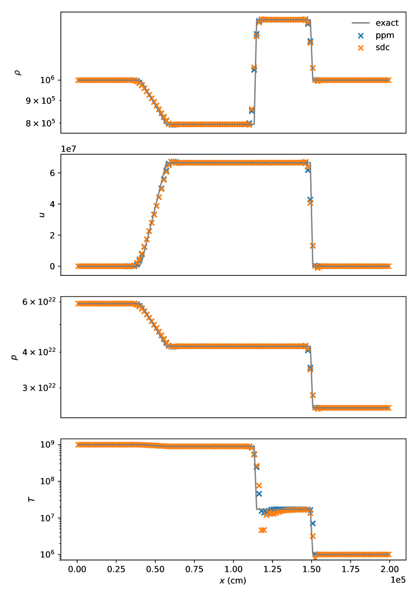
Figure 5: The stellar EOS strong shock problem (test 3) from Zingale & Katz (2015).

5.4 Thermal diffusion test

The standard test problem for thermal diffusion is to diffuse a Gaussian temperature profile with a constant diffusion coefficient, which remains Gaussian but with a lower amplitude and greater width as time evolves. However, we want to ensure we converge properly for a state-dependent conductivity. To test this, we use a simple powerlaw thermal conductivity:

$$k_{\mathrm{th}}={k_{\mathrm{th}}}_{0}T^{\nu}$$ (79)

We adopt ${k_{\mathrm{th}}}_{0}=1$ and $\nu=2$. We still begin with a Gaussian profile of the form:

$$T(r)=T_{1}+(T_{2}-T_{1})e^{-r^{2}/(4\mathcal{D}t_{0})}$$ (80)

where $r$ is the distance from the center of the domain, $\mathcal{D}$ is the thermal diffusivity,

$$\mathcal{D}=\frac{k_{\mathrm{th}}}{\rho c_{v}}$$ (81)

and $t_{0}$ has units of time and serves to control the initial width of the Gaussian. We take $t_{0}=10^{-3}~{}\mathrm{s}$ here, and turn off hydrodynamics, so only the temperature and internal energy evolve in this test. We use a gamma-law equation of state and a pure hydrogen composition (with $\gamma=5/3$), so the specific heat is just

$$c_{v}=\frac{3}{2}\frac{k_{B}}{m_{u}}$$ (82)

where $k_{B}$ is Boltzmann’s constant and $m_{u}$ is the atomic mass unit. We choose the constant density in the domain, $\rho_{0}$, so that the thermal diffusivity in the center is $\mathcal{D}(r=0)=1$. This gives:

$$\rho_{0}=\frac{k_{\mathrm{th}}(T_{2})}{c_{v}(T_{2})}$$ (83)

Finally, we use the standard explicit diffusion timestep limiter, of the form:

$$\delta t_{\mathrm{diff}}=\frac{\mathcal{C}}{2}\min\left\{\frac{\Delta x^{2}}{\mathcal{D}}\right\}$$ (84)

where we use the same CFL factor as with hydrodynamics to reduce the timestep.

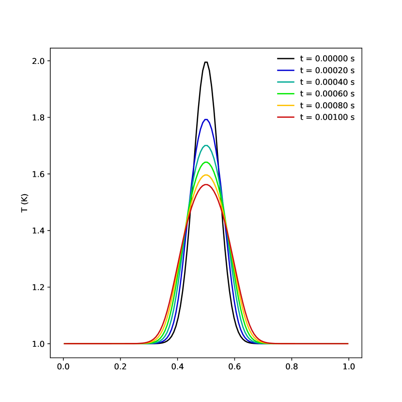
Figure 6: Temperature profiles for the 1-d thermal diffusion test run with 128 zones.

Table 5: Convergence ($L_{1}$ norm) for the 1-d and 2-d thermal diffusion test with fourth-order SDC.

field	$\epsilon_{64\rightarrow 128}$	rate	$\epsilon_{128\rightarrow 256}$	rate	$\epsilon_{256\rightarrow 512}$
1-d test
$\rho e$	$1.112\times 10^{-5}$	3.949	$7.198\times 10^{-7}$	3.987	$4.539\times 10^{-8}$
$T$	$1.063\times 10^{-5}$	3.953	$6.867\times 10^{-7}$	3.975	$4.368\times 10^{-8}$
2-d test
$\rho e$	$1.902\times 10^{-6}$	3.958	$1.224\times 10^{-7}$	3.987	$7.719\times 10^{-9}$
$T$	$1.770\times 10^{-6}$	3.966	$1.133\times 10^{-7}$	3.991	$7.127\times 10^{-9}$

We run in 1-d on a domain $[0,1]$, with 64, 128, 256, and 512 cells for $10^{-3}~{}\mathrm{s}$, with $\mathcal{C}=0.5$. Figure 6 shows the temperature profile at various times. Table 5 shows the convergence for the test in 1-d—we see nearly perfect fourth-order convergence. We also run in 2-d on $[0,1]^{2}$ with $64^{2}$, $128^{2}$, $256^{2}$, and $512^{2}$ cells for the same time. In 2-d, we exercise the face-averaging of the diffusive fluxes. The same table shows the convergence for 2-d, and again we see nearly perfect fourth-order convergence.

5.5 Reacting Hydrodynamics Test

Next we adapt the general EOS acoustic pulse problem from section 5.2 to include reactions, which enables us to test the convergence rate of the coupled hydrodynamics and reactions update. The problem setup is the same, but we now initialize the material to be completely ${}^{4}\mathrm{He}$ and we use a simple reaction network with the triple-alpha and ${}^{12}\mathrm{C}(\alpha,\gamma){}^{16}\mathrm{O}$ reactions, using rates from Caughlan & Fowler (1988) along with screening from Graboske et al. (1973); Alastuey & Jancovici (1978); Itoh et al. (1979). The network also contains ${}^{56}\mathrm{Fe}$, which is not linked to any other nuclei via reactions (it is used as an inert marker). This network is available as part of the StarKiller microphysics project (the StarKiller Microphysics Development Team et al., 2019). Since we start out as ${}^{4}\mathrm{He}$, any ${}^{12}\mathrm{C}$ or ${}^{16}\mathrm{O}$ in the final output is created via the nucleosynthesis, so these species can help understand the convergence of the reactions.

For all the SDC runs, we use the simple Newton solve, the analytic estimate of the Jacobian, solve for $(\rho e)$ in the update, and set the tolerances as ${\epsilon_{\mathrm{rel},\rho}}=10^{-10}$, ${\epsilon_{\mathrm{rel},(\rho X)}}=10^{-10}$, ${\epsilon_{\mathrm{rel},(\rho e)}}=10^{-5}$, and ${\epsilon_{\mathrm{abs}}}=10^{-10}$.

We run with the same timestep as the non-reacting version to a stop time of 0.06 s. Here we compute the convergence rate for the Strang CTU, SDC-2, and SDC-4 solvers. All simulations are run in 2-d.

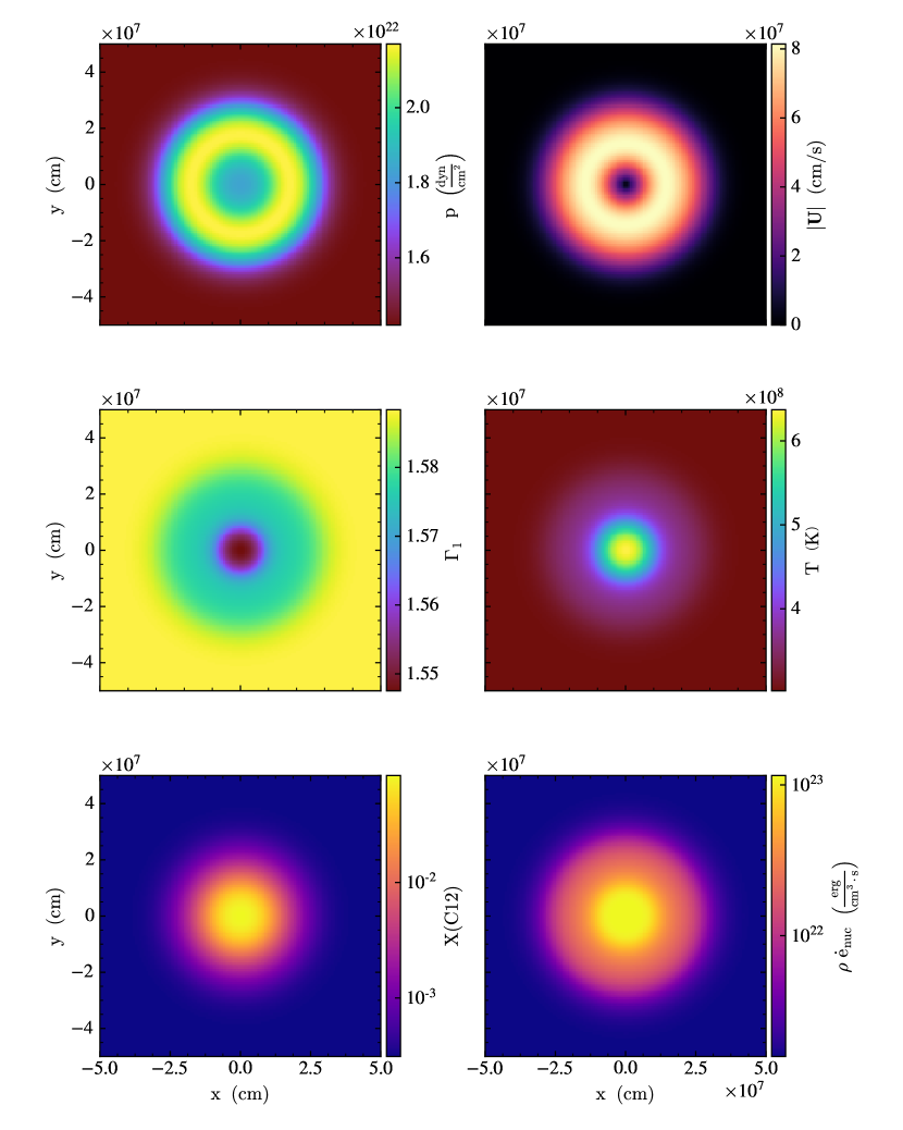
Figure 7: Thermodynamic, dynamic, and nuclear state at $t=0.06~{}\mathrm{s}$ for the reacting hydrodynamics test run with SDC-4 using $128^{2}$ cells.

Table 6: Convergence ($L_{1}$ norm) for the reacting convergence problem with the Strang CTU solver.

field	$\epsilon_{64\rightarrow 128}$	rate	$\epsilon_{128\rightarrow 256}$	rate	$\epsilon_{256\rightarrow 512}$
$\rho$	$2.780\times 10^{18}$	2.051	$6.706\times 10^{17}$	2.580	$1.121\times 10^{17}$
$\rho u$	$6.780\times 10^{26}$	2.446	$1.245\times 10^{26}$	2.907	$1.659\times 10^{25}$
$\rho v$	$6.780\times 10^{26}$	2.446	$1.245\times 10^{26}$	2.907	$1.659\times 10^{25}$
$\rho E$	$2.465\times 10^{35}$	2.333	$4.893\times 10^{34}$	2.650	$7.797\times 10^{33}$
$\rho e$	$2.268\times 10^{35}$	2.298	$4.611\times 10^{34}$	2.721	$6.991\times 10^{33}$
$T$	$2.245\times 10^{21}$	1.682	$6.995\times 10^{20}$	2.439	$1.290\times 10^{20}$
$\rho X({}^{4}\mathrm{He})$	$2.861\times 10^{18}$	2.027	$7.018\times 10^{17}$	2.553	$1.195\times 10^{17}$
$\rho X({}^{12}\mathrm{C})$	$1.717\times 10^{17}$	1.945	$4.458\times 10^{16}$	2.194	$9.745\times 10^{15}$
$\rho X({}^{16}\mathrm{O})$	$1.717\times 10^{14}$	1.648	$5.479\times 10^{13}$	1.898	$1.471\times 10^{13}$
$\rho X({}^{56}\mathrm{Fe})$	$2.780\times 10^{-12}$	2.051	$6.706\times 10^{-13}$	2.580	$1.121\times 10^{-13}$

Table 7: Convergence ($L_{1}$ norm) for the reacting convergence problem with the SDC-2 solver.

field	$\epsilon_{64\rightarrow 128}$	rate	$\epsilon_{128\rightarrow 256}$	rate	$\epsilon_{256\rightarrow 512}$
$\rho$	$2.024\times 10^{18}$	2.011	$5.022\times 10^{17}$	2.021	$1.238\times 10^{17}$
$\rho u$	$3.720\times 10^{26}$	2.063	$8.901\times 10^{25}$	2.030	$2.180\times 10^{25}$
$\rho v$	$3.720\times 10^{26}$	2.063	$8.901\times 10^{25}$	2.030	$2.180\times 10^{25}$
$\rho E$	$2.302\times 10^{35}$	2.030	$5.635\times 10^{34}$	2.014	$1.395\times 10^{34}$
$\rho e$	$2.053\times 10^{35}$	2.025	$5.043\times 10^{34}$	2.013	$1.249\times 10^{34}$
$T$	$1.643\times 10^{21}$	2.060	$3.939\times 10^{20}$	2.026	$9.676\times 10^{19}$
$\rho X({}^{4}\mathrm{He})$	$2.002\times 10^{18}$	2.015	$4.951\times 10^{17}$	2.027	$1.215\times 10^{17}$
$\rho X({}^{12}\mathrm{C})$	$1.042\times 10^{17}$	2.032	$2.546\times 10^{16}$	2.019	$6.281\times 10^{15}$
$\rho X({}^{16}\mathrm{O})$	$1.564\times 10^{14}$	1.935	$4.090\times 10^{13}$	2.003	$1.020\times 10^{13}$
$\rho X({}^{56}\mathrm{Fe})$	$2.024\times 10^{-12}$	2.011	$5.022\times 10^{-13}$	2.021	$1.238\times 10^{-13}$

Table 8: Convergence ($L_{1}$ norm) for the reacting convergence problem with the SDC-4 solver.

field	$\epsilon_{64\rightarrow 128}$	rate	$\epsilon_{128\rightarrow 256}$	rate	$\epsilon_{256\rightarrow 512}$
$\rho$	$2.127\times 10^{17}$	3.855	$1.470\times 10^{16}$	3.972	$9.369\times 10^{14}$
$\rho u$	$3.401\times 10^{25}$	3.856	$2.349\times 10^{24}$	3.958	$1.511\times 10^{23}$
$\rho v$	$3.401\times 10^{25}$	3.856	$2.349\times 10^{24}$	3.958	$1.511\times 10^{23}$
$\rho E$	$1.945\times 10^{34}$	3.891	$1.311\times 10^{33}$	3.953	$8.463\times 10^{31}$
$\rho e$	$1.672\times 10^{34}$	3.899	$1.120\times 10^{33}$	3.955	$7.223\times 10^{31}$
$T$	$1.236\times 10^{20}$	3.708	$9.463\times 10^{18}$	3.949	$6.125\times 10^{17}$
$\rho X({}^{4}\mathrm{He})$	$2.147\times 10^{17}$	3.858	$1.481\times 10^{16}$	3.969	$9.458\times 10^{14}$
$\rho X({}^{12}\mathrm{C})$	$8.789\times 10^{15}$	3.798	$6.319\times 10^{14}$	3.911	$4.201\times 10^{13}$
$\rho X({}^{16}\mathrm{O})$	$1.294\times 10^{13}$	3.765	$9.518\times 10^{11}$	3.872	$6.501\times 10^{10}$
$\rho X({}^{56}\mathrm{Fe})$	$2.127\times 10^{-13}$	3.855	$1.470\times 10^{-14}$	3.972	$9.369\times 10^{-16}$

Figure 7 shows the thermodynamic, dynamic, and nuclear state for the $128^{2}$ SDC-4 simulation at 0.06 s. We run with $64^{2}$, $128^{2}$, $256^{2}$, and $512^{2}$ cells and compute the error between successive resolutions and measure the convergence rate. Tables 6, 7, and 8 show the convergence. We see that the Strang CTU algorithm achieves second order for most variables (as expected), with some quantities converging almost third order (for smooth flows, the PPM algorithm approaches third order accuracy in space), while having difficulty with ${}^{16}\mathrm{O}$. For SDC-2, we see second-order convergence in all the variables, including ${}^{16}\mathrm{O}$. Finally, for SDC-4, all of the variables converge at rates of $\sim 3.8$–$3.9$, demonstrating the fourth-order accuracy expected for the method. This test shows that the SDC algorithm can achieve fourth-order convergence for reactive hydrodynamics problems with astrophysical networks.

5.6 Burning Buoyant Bubble

Our final convergence test problem considers a hydrostatic atmosphere with a temperature perturbuation. Buoyancy causes the perturbation to rise (and eventually roll up in the nonlinear phase). The presence of reactions prevents the bubble from fizzling out, keeping it buoyant via the heat deposition. In addition to looking at the convergence rate of the numerical solutions, we also consider how well we maintain hydrostatic equilibrium in an undisturbed hydrostatic atmosphere.

We create an initial atmospheric model that is isentropic and in hydrostatic equilibrium by integrating the system:

$$\frac{dp}{dy} =-\rho(p,s)g$$ (85)

$$\frac{ds}{dy} =0$$ (86)

where the relation $\rho(p,s)$ is provided by our equation of state. We take gravity, $g$, to be constant and the composition to be uniform throughout the atmosphere (pure helium, with the other nuclei mass fractions set to the small value $10^{-8}$). To integrate this system, we specify the conditions at the base of the atmosphere, which we take to be the lower domain boundary (not the center of the bottom-most cell). We specify $\rho_{\mathrm{base}}$, and $T_{\mathrm{base}}$ and get $p_{\mathrm{base}}$ and $s_{\mathrm{base}}$ through the general stellar equation of state. We integrate this system using fourth-order Runge-Kutta, using a step size of $\Delta x/2$ to get from the bottom of the domain to the first cell-center, and then a step size of $\Delta x$ to integrate to each of the remaining cell-centers vertically in the domain. The initial conditions are then converted to cell-averages using the same transformation discussed earlier in the paper. Note: the hydrostatic model is generated specifically for the resolution of the problem, and as such, the initial atmosphere converges with fourth-order accuracy. For the boundary conditions, we use periodic conditions on the sides and reflecting boundary conditions at the top and bottom. Table 9 lists the problem setup parameters.

Table 9: Hydrostatic atmosphere initial condition parameters.

parameter	value
$\rho_{\mathrm{base}}$	$10^{7}~{}\mathrm{g~{}cm^{-3}}$
$T_{\mathrm{base}}$	$10^{8}~{}\mathrm{K}$
$g$	$10^{10}~{}\mathrm{cm~{}s^{-2}}$
$L_{x}=L_{y}$ (domain size)	$7.68\times 10^{6}~{}\mathrm{cm}$
$\sigma$	$2.56\times 10^{5}~{}\mathrm{cm}$

To test this initial setup, we evolve just the hydrostatic atmosphere on our 2-d grid. Analytically, the velocity should remain zero, if hydrostatic equilibrium cancellation were perfect. Due to truncation error, a velocity does build up over time, so we use the maximum of the velocity magnitude, $|\mathbf{U}|$, as the measure of the error. Table 10 lists this error for several resolutions. We note that the velocity magnitudes are quite small, and we also see fourth-order convergence as we increase the resolution. This suggests that with the fourth-order method, we can accurately maintain an atmosphere in HSE without the need for well-balanced schemes (Zingale et al., 2002; Käppeli & Mishra, 2016).

Table 10: Convergence of $\max\{|\mathbf{U}|\}$ for an unperturbed hydrostatic atmosphere with fourth-order SDC.

$64^{2}$	rate	$128^{2}$	rate	$256^{2}$
$1.884\times 10^{-2}$	3.987	$1.188\times 10^{-3}$	3.825	$8.383\times 10^{-5}$

Next we add a perturbation and enable reactions, using the same $3$-$\alpha$ + ${}^{12}\mathrm{C}(\alpha,\gamma){}^{16}\mathrm{O}$ network described above. To perturb the atmosphere, we modify the temperature as:

$$T(x,y)=T_{0}(y)\left\{1+\frac{3}{5}\left[1+\tanh(4-r)\right]\right\}$$ (87)

where $T_{0}$ is the temperature of the initial hydrostatic atmosphere at the height $y$, and $r$ is the distance from the center of the domain. The amplitude of the perturbation was chosen to give a reasonable amount of burning to ${}^{12}\mathrm{C}$ while keeping the Mach number below 0.1, while the shape was chosen to give a flat central region. We then recompute the pressure at each point in the atmosphere through the equation of state, constraining it to the hydrostatic pressure at the altitude, $p(y)$:

$$\rho(x,y)=\rho(T(x,y),p(y))$$ (88)

This reduces the density, creating the initial buoyancy. We run on domains $64^{2}$, $128^{2}$, $256^{2}$, and $512^{2}$, to $0.1~{}\mathrm{s}$ using a fixed timestep:

$$\delta t=1.5\times 10^{-4}\left(\frac{64}{n_{\mathrm{zones}}}\right)~{}\mathrm{s}.$$ (89)

This is a difficult test problem because of the extreme nonlinearily of the dynamics. The end time is picked so we measure convergence before the bubble begins to roll-up in a strongly nonlinear fashion. If we ran longer, the strong temperature dependence of the $3$-$\alpha$ burning would give strong nonlinear energy generation from local hot spots, making a convergence test difficult for the lowest resolution simulations we consider here.

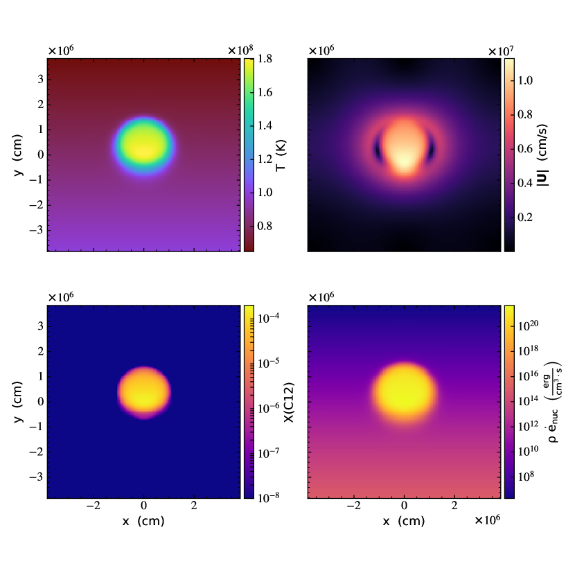
Figure 8: Final state of the burning buoyant bubble problem for the $128^{2}$ simulation.

Figure 8 shows the state of the bubble at the end point. Table 11 shows the convergence across these problem sizes. At the lowest resolution, we barely resolve the burning region, which affects the convergence, but we see nearly fourth-order convergence for the higher resolution simulations. Again, this test demonstrates our SDC-4 method works as expected.

Table 11: Convergence ($L_{1}$ norm) for the burning buoyant bubble problem using the SDC-4 solver.

field	$\epsilon_{64\rightarrow 128}$	rate	$\epsilon_{128\rightarrow 256}$	rate	$\epsilon_{256\rightarrow 512}$
$\rho$	$3.591\times 10^{15}$	3.263	$3.739\times 10^{14}$	3.713	$2.852\times 10^{13}$
$\rho u$	$1.120\times 10^{24}$	3.794	$8.072\times 10^{22}$	3.930	$5.296\times 10^{21}$
$\rho v$	$1.314\times 10^{24}$	3.544	$1.127\times 10^{23}$	3.838	$7.879\times 10^{21}$
$\rho E$	$3.701\times 10^{32}$	2.946	$4.801\times 10^{31}$	3.647	$3.834\times 10^{30}$
$\rho e$	$3.701\times 10^{32}$	2.946	$4.801\times 10^{31}$	3.646	$3.834\times 10^{30}$
$T$	$1.438\times 10^{18}$	3.508	$1.264\times 10^{17}$	3.829	$8.899\times 10^{15}$
$\rho X({}^{4}\mathrm{He})$	$3.589\times 10^{15}$	3.266	$3.732\times 10^{14}$	3.711	$2.850\times 10^{13}$
$\rho X({}^{12}\mathrm{C})$	$1.520\times 10^{13}$	2.544	$2.606\times 10^{12}$	3.797	$1.874\times 10^{11}$
$\rho X({}^{16}\mathrm{O})$	$3.589\times 10^{7}$	3.262	$3.742\times 10^{6}$	3.714	$2.851\times 10^{5}$
$\rho X({}^{56}\mathrm{Fe})$	$3.590\times 10^{7}$	3.263	$3.739\times 10^{6}$	3.713	$2.852\times 10^{5}$

5.7 Proof-of-concept: Helium deflagration

To demonstrate that the SDC methods work with more extensive networks, we run a 1-d helium deflagration with a 13 isotope alpha network, using conditions that are appropriate to an sub-Chandra model of Type Ia supernovae. We do not try to assess convergence of the flame here, because of the large number of timesteps ($\sim 10^{6}$) needed to get ignition and the extreme nonlinearity of the burning. Instead, we wish to demonstrate that the SDC-4 method can evolve a flame using only the simple Newton iterations for the solution instead of needing to solve an ODE system as we do with Strang-split methods.

We start by defining a fuel state in terms of density, temperature, and composition: $\rho_{\mathrm{fuel}}$, $T_{\mathrm{fuel}}$, $X_{\mathrm{fuel}}$. From these conditions, we define an ambient pressure through the equation of state:

$$p_{\mathrm{ambient}}=p(\rho_{\mathrm{fuel}},T_{\mathrm{fuel}},X_{\mathrm{fuel}})$$ (90)

We keep the pressure constant throughout the domain. We then define an ash temperature and composition, $T_{\mathrm{ash}}$ and $X_{\mathrm{ash}}$, and we smoothly transition from the fuel to ash state as:

$$T =T_{\mathrm{fuel}}+\frac{1}{2}(T_{\mathrm{ash}}-T_{\mathrm{fuel}})\left[1-\tanh\left(\frac{x-x_{\mathrm{int}}}{\delta_{\mathrm{blend}}}\right)\right]$$ (91)

$$X_{k} =X_{\mathrm{fuel},k}+\frac{1}{2}(X_{\mathrm{ash},k}-X_{\mathrm{fuel},k})\left[1-\tanh\left(\frac{x-x_{\mathrm{int}}}{\delta_{\mathrm{blend}}}\right)\right]$$ (92)

and find the ash density by constraining the conditions to be isobaric with the fuel through the equation of state:

$$\rho_{\mathrm{ash}}=\rho(p_{\mathrm{ambient}},T_{\mathrm{ash}},X_{\mathrm{ash}})$$ (93)

Here, $x_{\mathrm{int}}$ is the location of the initial transition between ash (on the left) and fuel (on the right), and $\delta_{\mathrm{blend}}$ is the width of the transition. The remaining thermodynamic quantities are found via the equation of state. We use a domain $[0,L_{x}]$ with simple zero-gradient boundary conditions. The parameters used for our simulation are shown in Table 12.

Table 12: Helium flame initial condition parameters.

parameter	value
$\rho_{\mathrm{fuel}}$	$2\times 10^{7}~{}\mathrm{g~{}cm^{-3}}$
$T_{\mathrm{fuel}}$	$5\times 10^{7}~{}\mathrm{K}$
$X_{\mathrm{fuel}}({}^{4}\mathrm{He})$	1.0
$T_{\mathrm{ash}}$	$3.6\times 10^{9}~{}\mathrm{K}$
$X_{\mathrm{ash}}({}^{56}\mathrm{Ni})$	1.0
$L_{x}$	$256~{}\mathrm{cm}$
$x_{\mathrm{int}}$	$0.4L_{x}$
$\delta_{\mathrm{blend}}$	$0.06L_{x}$

We use the Newton solver with an analytic Jacobian. We set the tolerances as: ${\epsilon_{\mathrm{rel},\rho}}=10^{-10}$, ${\epsilon_{\mathrm{rel},(\rho X)}}=10^{-10}$, ${\epsilon_{\mathrm{rel},(\rho e)}}=10^{-6}$, and ${\epsilon_{\mathrm{abs}}}=10^{-10}$. We run with an advective CFL number of $\mathcal{C}=0.75$ and use 256 zones. We also use the diffusion limiter described above (Eq. 84), and an additional limiter based on the nuclear energy generation rate, which helps reduce the timestep right as the flame is igniting. This sets the timestep to be:

$$\delta t_{\mathrm{nuc}}=\zeta\frac{e}{\dot{S}}$$ (94)

The idea is to not let nuclear reactions change a cell’s internal energy, $e$, by more than a fraction $\zeta$. We use $\zeta=0.25$ for these simulations. It is still possible for rapidly increasing energy generation to violate this limiter, since we use the current timestep’s state to predict the $\delta t_{\mathrm{nuc}}$ for the next step.

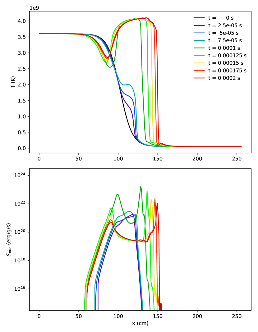
Figure 9: A helium flame run with the SDC-4 algorithm.

Figure 9 shows the temperature and energy generation rate in flame at several instances in time, We see that diffusion and reactions slowly increase the temperature at the fuel-ash interface during the early evolution before the flame rapidly ignites. At the final point in the evolution, the flame still has not reached a steady state. This problem demonstrates that the SDC-4 algorithm works well with more extensive networks.

6 Summary

We showed that spectral deferred corrections can lead to high-order coupling of hydrodynamics and reactions for astrophysical problems. Aside from the shock tubes and example flame, we focused on smooth problems so we could measure convergence. We saw that we can achieve fourth-order convergence in reacting flow problems with stiff reaction sources using the SDC coupling. This work provides a path for doing multiphysics time evolution to higher than second-order temporal accuracy. Extensions to this include self-gravity, including the conservative formulation described in Katz et al. (2016). We would need to solve the Poisson equation at each time node, for each iteration. Using geometric multigrid, we would expect the later iterations to converge quickly when we start with the potential from the previous iteration. There are also extensions to radiation, like that explored to second-order in Sekora & Stone 2009. Finally, we will expand this methodology adaptive mesh refinement with subcycling in time.

In a follow-on paper, we will explore burning fronts more thoroughly, including deflagrations and detonations, where it has been shown that resolution is key to avoiding spurious numerically-seeded detonations (Katz & Zingale, 2019), so higher-order methods may help. We also want to understand how the improved coupling helps with nuclear statistical equilibrium attained in the ashes. Finally, our main science target is modeling flame spreading in X-ray bursts, where the wide range of length scales makes resolved simulations challenging (Zingale et al., 2019), so the push to fourth-order reactive hydrodynamics should help. We’ve demonstrated that we have the necessary physics to fourth-order accuracy for our models of X-ray bursts. We focused on Cartesian geometry here. The extension to axisymmetric flows is straightforward, but requires deriving the fourth-order interpolants in that geometry. We will consider that in a separate study.

It is straightforward to adapt an existing method-of-lines hydrodynamics code to use this SDC integration technique. The main piece needed is access to the instantaneous reaction rates, instead of relying on a network integration package. The methodology presented here can also be extended to radiation and implicit diffusion to enable higher time-order and better coupling, and could be useful as well for fully implicit hydrodynamics schemes, including those used by stellar evolution codes. It can also be easily adapted to cosmological flows with chemistry. Finally, there are a large number of variations on the SDC approach shown here. We could use a different quadrature rule for the integral or subcycle on the reactions, if needed. We will explore variations in future papers.

Appendix A Jacobian

For solving the nonlinear update of the reacting system, we need to compute the Jacobian, $\partial{\bf R}/\partial{\,\bm{\mathcal{U}}}$. We do this in two pieces, $\partial{\bf R}/\partial{\bf w}$ and $\partial{\bf w}/\partial{\,\bm{\mathcal{U}}}$. We will show two species here, called $X_{\alpha}$ and $X_{\beta}$, so the structure of the matricies is clear when there are multiple species. We need to compute $\partial{\bf w}/\partial{\,\bm{\mathcal{U}}}$, with ${\bf w}=(\rho,X_{\alpha},X_{\beta},T)^{\intercal}$. For this transformation, we need to pick only one of $(\rho E)$ or $(\rho e)$. We show the Jacobian for both choices, denoting the state as ${\,\bm{\mathcal{U}}}_{(E)}$ when we include $(\rho E)$ and as ${\,\bm{\mathcal{U}}}_{(e)}$ when we include $(\rho e)$,

$${\,\bm{\mathcal{U}}}_{(E)}=\left(\begin{array}[]{c}\rho\\ \rho X_{\alpha}\\ \rho X_{\beta}\\ \rho E\end{array}\right)\quad{\,\bm{\mathcal{U}}}_{(e)}=\left(\begin{array}[]{c}\rho\\ \rho X_{\alpha}\\ \rho X_{\beta}\\ \rho e\end{array}\right)$$ (A1)

The Jacobian transformation $\partial{\,\bm{\mathcal{U}}}/\partial{\bf w}$ for each of these conserved state choices can be written down straightforwardly as:

$$\frac{\partial{\,\bm{\mathcal{U}}}_{(E)}}{\partial{\bf w}}=\left(\begin{array}[]{cccc}1&0&0&0\\ X_{\alpha}&\rho&0&0\\ X_{\beta}&0&\rho&0\\ \rho e_{\rho}+e+\frac{1}{2}\mathbf{U}^{2}&\rho e_{X_{\alpha}}&\rho e_{X_{\beta}}&\rho e_{T}\end{array}\right)\quad\frac{\partial{\,\bm{\mathcal{U}}}_{(e)}}{\partial{\bf w}}=\left(\begin{array}[]{cccc}1&0&0&0\\ X_{\alpha}&\rho&0&0\\ X_{\beta}&0&\rho&0\\ \rho e_{\rho}+e&\rho e_{X_{\alpha}}&\rho e_{X_{\beta}}&\rho e_{T}\end{array}\right)$$ (A2)

where we use the following notation for compactness:

$$e_{\rho}=\left.\frac{\partial{}e}{\partial\rho}\right|_{T,X_{k}}\qquad e_{T}=\left.\frac{\partial{}e}{\partial{}T}\right|_{\rho,X_{k}}\qquad e_{X_{k}}=\left.\frac{\partial{}e}{\partial{}X_{k}}\right|_{\rho,T,X_{j,j\neq k}}$$ (A3)

and the inverses (computed via SymPy, see the included Jupyter notebook) are:

$$\frac{\partial{\bf w}}{\partial{\,\bm{\mathcal{U}}}_{(E)}}=\left(\begin{array}[]{cccc}1&0&0&0\\ -\frac{X_{\alpha}}{\rho}&\frac{1}{\rho}&0&0\\ -\frac{X_{\beta}}{\rho}&0&\frac{1}{\rho}&0\\ \left(\rho e_{T}\right)^{-1}\left(\sum_{k}X_{k}e_{X_{k}}-\rho e_{\rho}-e+\frac{1}{2}\mathbf{U}^{2}\right)&-\frac{e_{X_{\alpha}}}{\rho e_{T}}&-\frac{e_{X_{\beta}}}{\rho e_{T}}&\frac{1}{\rho e_{T}}\end{array}\right)$$ (A4)

and

$$\frac{\partial{\bf w}}{\partial{\,\bm{\mathcal{U}}}_{(e)}}=\left(\begin{array}[]{cccc}1&0&0&0\\ -\frac{X_{\alpha}}{\rho}&\frac{1}{\rho}&0&0\\ -\frac{X_{\beta}}{\rho}&0&\frac{1}{\rho}&0\\ \left(\rho e_{T}\right)^{-1}\left(\sum_{k}X_{k}e_{X_{k}}-\rho e_{\rho}-e\right)&-\frac{e_{X_{\alpha}}}{\rho e_{T}}&-\frac{e_{X_{\beta}}}{\rho e_{T}}&\frac{1}{\rho e_{T}}\end{array}\right)$$ (A5)

The reaction vector is the same regardless of the choice of $(\rho E)$ or $(\rho e)$, as

$${\bf R}=\left(\begin{array}[]{c}0\\ \rho\dot{\omega}_{\alpha}\\ \rho\dot{\omega}_{\beta}\\ \rho\dot{S}\end{array}\right)$$ (A6)

and the Jacobian is computed as $\partial{\bf R}/\partial{\bf w}$:

$$\frac{\partial{\bf R}}{\partial{\bf w}}=\left(\begin{array}[]{cccc}0&0&0&0\\ \dot{\omega}_{\alpha}+\rho\frac{\partial\dot{\omega}_{\alpha}}{\partial\rho}&\rho\frac{\partial\dot{\omega}_{\alpha}}{\partial X_{\alpha}}&\rho\frac{\partial\dot{\omega}_{\alpha}}{\partial X_{\beta}}&\rho\frac{\partial\dot{\omega}_{\alpha}}{\partial T}\\ \dot{\omega}_{\beta}+\rho\frac{\partial\dot{\omega}_{\beta}}{\partial\rho}&\rho\frac{\partial\dot{\omega}_{\beta}}{\partial X_{\alpha}}&\rho\frac{\partial\dot{\omega}_{\beta}}{\partial X_{\beta}}&\rho\frac{\partial\dot{\omega}_{\beta}}{\partial T}\\ \dot{S}+\rho\frac{\partial\dot{S}}{\partial\rho}&\rho\frac{\partial\dot{S}}{\partial X_{\alpha}}&\rho\frac{\partial\dot{S}}{\partial X_{\beta}}&\rho\frac{\partial\dot{S}}{\partial T}\\ \end{array}\right)$$ (A7)

The first row of zeros is not as alarming as it looks, since the full Jacobian has the form ${\bf J}={\bf I}-\delta t_{m}(\partial{\bf R}/\partial{\bf w})(\partial{\bf w}/\partial{\,\bm{\mathcal{U}}})$.

References

- Alastuey & Jancovici (1978) Alastuey, A., & Jancovici, B. 1978, ApJ, 226, 1034, doi: 10.1086/156681
- Almgren et al. (2013) Almgren, A., Aspden, A., Bell, J., & Minion, M. 2013, SIAM Journal on Scientific Computing, 35, B25, doi: 10.1137/110829386
- Almgren et al. (2008) Almgren, A. S., Bell, J. B., Nonaka, A., & Zingale, M. 2008, ApJ, 684, 449, doi: 10.1086/590321
- Almgren et al. (2010) Almgren, A. S., Beckner, V. E., Bell, J. B., et al. 2010, ApJ, 715, 1221, doi: 10.1088/0004-637X/715/2/1221
- Bourlioux et al. (2003) Bourlioux, A., Layton, A. T., & Minion, M. L. 2003, Journal of Computational Physics, 189, 651 , doi: https://doi.org/10.1016/S0021-9991(03)00251-1
- Brown et al. (1989) Brown, P., Byrne, G., & Hindmarsh, A. 1989, SIAM Journal on Scientific and Statistical Computing, 10, 1038, doi: 10.1137/0910062
- Bruenn et al. (2018) Bruenn, S. W., Blondin, J. M., Hix, W. R., et al. 2018, arXiv e-prints, arXiv:1809.05608. https://arxiv.org/abs/1809.05608
- Bryan et al. (1995) Bryan, G. L., Norman, M. L., Stone, J. M., Cen, R., & Ostriker, J. P. 1995, Computer Physics Communications, 89, 149, doi: 10.1016/0010-4655(94)00191-4
- Byrne & Hindmarsh (1987) Byrne, G. D., & Hindmarsh, A. C. 1987, Journal of Computational Physics, 70, 1 , doi: https://doi.org/10.1016/0021-9991(87)90001-5
- Caughlan & Fowler (1988) Caughlan, G. R., & Fowler, W. A. 1988, Atomic Data and Nuclear Data Tables, 40, 283, doi: 10.1016/0092-640X(88)90009-5
- Colella (1985) Colella, P. 1985, SIAM Journal on Scientific and Statistical Computing, 6, 104, doi: 10.1137/0906009
- Colella (1990) Colella, P. 1990, Journal of Computational Physics, 87, 171, doi: 10.1016/0021-9991(90)90233-Q
- Dutt et al. (2000) Dutt, A., Greengard, L., & Rokhlin, V. 2000, BIT Numerical Mathematics, 40, 241, doi: 10.1023/A:102233890
- Emmett et al. (2019) Emmett, M., Motheau, E., Zhang, W., Minion, M., & Bell, J. B. 2019, Combustion Theory and Modelling, 23, 592, doi: 10.1080/13647830.2019.1566574
- Emmett et al. (2014) Emmett, M., Zhang, W., & Bell, J. B. 2014, Combustion Theory and Modelling, 18, 361, doi: 10.1080/13647830.2014.919410
- Felker & Stone (2018) Felker, K. G., & Stone, J. M. 2018, Journal of Computational Physics, 375, 1365, doi: 10.1016/j.jcp.2018.08.025
- Fryxell et al. (2000) Fryxell, B., Olson, K., Ricker, P., et al. 2000, ApJS, 131, 273, doi: 10.1086/317361
- Graboske et al. (1973) Graboske, H. C., Dewitt, H. E., Grossman, A. S., & Cooper, M. S. 1973, ApJ, 181, 457
- Harpole et al. (2019) Harpole, A., Zingale, M., Hawke, I., & Chegini, T. 2019, Journal of Open Source Software, 4, 1265, doi: 10.21105/joss.01265
- Huang et al. (2006) Huang, J., Jia, J., & Minion, M. 2006, Journal of Computational Physics, 214, 633
- Hunter (2007) Hunter, J. D. 2007, Computing in Science and Engg., 9, 90, doi: 10.1109/MCSE.2007.55
- Itoh et al. (1979) Itoh, N., Totsuji, H., Ichimaru, S., & Dewitt, H. E. 1979, ApJ, 234, 1079, doi: 10.1086/157590
- Jones et al. (2001–) Jones, E., Oliphant, T., Peterson, P., et al. 2001–, SciPy: Open source scientific tools for Python. http://www.scipy.org/
- Kadioglu et al. (2008) Kadioglu, S. Y., Klein, R., & Minion, M. L. 2008, Journal of Computational Physics, 227, 2012 , doi: https://doi.org/10.1016/j.jcp.2007.10.008
- Käppeli & Mishra (2016) Käppeli, R., & Mishra, S. 2016, A&A, 587, A94, doi: 10.1051/0004-6361/201527815
- Katz & Zingale (2019) Katz, M. P., & Zingale, M. 2019, ApJ, 874, 169, doi: 10.3847/1538-4357/ab0c00
- Katz et al. (2016) Katz, M. P., Zingale, M., Calder, A. C., et al. 2016, ApJ, 819, 94, doi: 10.3847/0004-637X/819/2/94
- McCorquodale & Colella (2011) McCorquodale, P., & Colella, P. 2011, Commun. Appl. Math. Comput. Sci., 6, 1, doi: 10.2140/camcos.2011.6.1
- Meakin & Arnett (2007) Meakin, C. A., & Arnett, D. 2007, ApJ, 667, 448, doi: 10.1086/520318
- Meurer et al. (2017) Meurer, A., Smith, C. P., Paprocki, M., et al. 2017, PeerJ Computer Science, 3, e103, doi: 10.7717/peerj-cs.103
- Miller & Colella (2002) Miller, G. H., & Colella, P. 2002, Journal of Computational Physics, 183, 26, doi: 10.1006/jcph.2002.7158
- Minion (2003) Minion, M. L. 2003, Commun. Math. Sci., 1, 471. https://projecteuclid.org:443/euclid.cms/1250880097
- Most et al. (2019) Most, E. R., Papenfort, L. J., & Rezzolla, L. 2019, arXiv e-prints, arXiv:1907.10328. https://arxiv.org/abs/1907.10328
- Müller (1986) Müller, E. 1986, A&A, 162, 103
- Nethercote & Seward (2007) Nethercote, N., & Seward, J. 2007, in Proceedings of the 28th ACM SIGPLAN Conference on Programming Language Design and Implementation, PLDI ’07 (New York, NY, USA: ACM), 89–100, doi: 10.1145/1250734.1250746
- Nonaka et al. (2010) Nonaka, A., Almgren, A. S., Bell, J. B., et al. 2010, ApJS, 188, 358, doi: 10.1088/0067-0049/188/2/358
- Oliphant (2007) Oliphant, T. E. 2007, Computing in Science and Engg., 9, 10, doi: 10.1109/MCSE.2007.58
- Pazner et al. (2016) Pazner, W. E., Nonaka, A., Bell, J. B., Day, M. S., & Minion, M. L. 2016, Combustion Theory and Modelling, 20, 521, doi: 10.1080/13647830.2016.1150519
- Sekora & Stone (2009) Sekora, M., & Stone, J. 2009, Communications in Applied Mathematics and Computational Science, 4, 135, doi: 10.2140/camcos.2009.4.135
- Strang (1968) Strang, G. 1968, SIAM Journal on Numerical Analysis, 5, 506, doi: 10.1137/0705041
- the AMReX Development Team et al. (2019) the AMReX Development Team, Almgren, A., Beckner, V., et al. 2019, AMReX-Codes/amrex: AMReX 19.08, doi: 10.5281/zenodo.3358046
- the Castro Development Team et al. (2019) the Castro Development Team, Almgren, A., Barrios Sazo, M., et al. 2019, AMReX-Astro/Castro: Castro 19.08.1, doi: 10.5281/zenodo.3359184
- the StarKiller Microphysics Development Team et al. (2019) the StarKiller Microphysics Development Team, Bishop, A., Fields, C. E., et al. 2019, starkiller-astro/Microphysics: StarKiller Microphysics 19.08, doi: 10.5281/zenodo.3357970
- Timmes & Swesty (2000) Timmes, F. X., & Swesty, F. D. 2000, ApJS, 126, 501, doi: 10.1086/313304
- Turk et al. (2011) Turk, M. J., Smith, B. D., Oishi, J. S., et al. 2011, ApJS, 192, 9, doi: 10.1088/0067-0049/192/1/9
- van der Walt et al. (2011) van der Walt, S., Colbert, S. C., & Varoquaux, G. 2011, Computing in Science & Engineering, 13, 22, doi: 10.1109/MCSE.2011.37
- Wongwathanarat et al. (2016) Wongwathanarat, A., Grimm-Strele, H., & Müller, E. 2016, A&A, 595, A41, doi: 10.1051/0004-6361/201628205
- Zhang et al. (2019) Zhang, W., Almgren, A., Beckner, V., et al. 2019, Journal of Open Source Software, 4, 1370, doi: 10.21105/joss.01370
- Zingale (2014) Zingale, M. 2014, Astronomy and Computing, 6, 52, doi: 10.1016/j.ascom.2014.07.003
- Zingale & Katz (2015) Zingale, M., & Katz, M. P. 2015, ApJS, 216, 31, doi: 10.1088/0067-0049/216/2/31
- Zingale et al. (2002) Zingale, M., Dursi, L. J., ZuHone, J., et al. 2002, ApJS, 143, 539, doi: 10.1086/342754
- Zingale et al. (2019) Zingale, M., Eiden, K., Cavecchi, Y., et al. 2019, Journal of Physics: Conference Series, 1225, 012005, doi: 10.1088/1742-6596/1225/1/012005