Detecting Heterogeneous Treatment Effect with Instrumental Variables
Abstract
There is an increasing interest in estimating heterogeneity in causal effects in randomized and observational studies. However, little research has been conducted to understand effect heterogeneity in an instrumental variables study. In this work, we present a method to estimate heterogeneous causal effects using an instrumental variable with matching. The method has two parts. The first part uses subject-matter knowledge and interpretable machine learning techniques, such as classification and regression trees, to discover potential effect modifiers. The second part uses closed testing to test for statistical significance of each effect modifier while strongly controlling the familywise error rate. We apply this method on the Oregon Health Insurance Experiment, estimating the effect of Medicaid on the number of days an individual’s health does not impede their usual activities by using a randomized lottery as an instrument. Our method revealed Medicaid’s effect was most impactful among older, English-speaking, non-Asian males and younger, English-speaking individuals with at most high school diplomas or General Educational Developments.
Keywords: Complier Average Causal Effect, Heterogeneous Treatment, Instrumental Variables, Matching, Machine Learning, Oregon Health Insurance Experiment
1 Introduction
1.1 Motivation: Utilization of Medicaid in Oregon and the Complier Average Treatment Effect
In January of 2008, Oregon reopened its Medicaid-based health insurance plan for its eligible residents and, for a brief period, allowed a limited number of individuals to enroll in the program. Specifically, a household in Oregon was randomly selected by a lottery system run by the state and any eligible individual in the household can choose to enroll in the new health insurance plan; households that weren’t selected by the lottery could not enroll whatsoever.
For policymakers, Oregon’s randomized lottery system was a unique opportunity, specifically a natural experiment, to study Medicaid’s causal effect on a variety of health and economic outcomes, as directly randomizing Medicaid (or withholding it) to individuals would be infeasible and unethical. In this natural experiment, commonly referred to as the Oregon Health Insurance Experiment (OHIE), Finkelstein et al., (2012) used the randomized lottery as an instrumental variable (see Section 2.2 for details) to study the complier average causal effect (CACE), or the effect of Medicaid among individuals who enrolled in Medicaid after winning the lottery (Angrist et al.,, 1996). The CACE reflects Medicaid’s impact among a subgroup of individuals and differs from the average treatment effect for the entire population (ATE) or the intent-to-treat (ITT) effect of the lottery itself on the outcome. In this paper, we focus on studying the CACE; see Imbens, (2010), Swanson and Hernán, (2013), and Swanson and Hernán, (2014) for additional discussions on the CACE.
Often in studying the CACE, the population of compliers is assumed to be homogeneous whereby two compliers are alike and have the same treatment effect. But, no two individuals are the same and it is plausible that some compliers may benefit more from the treatment than other compliers. For example, sick individuals who enroll in Medicaid after winning the lottery may benefit more from Medicaid than healthy individuals. Also, the perceived benefit of enrolling in Medicaid among sick versus healthy individuals may create heterogeneity in the compliance rate, i.e. the number of people who sign up when they win the lottery, with sick people presumably signing up more than healthy people. Alternatively, if people are equally likely to enroll in Medicaid when they win the lottery, those who are unemployed may benefit more from Medicaid in terms of reducing out-of-pocket healthcare spending and medical debt than those who are employed. The theme of this paper is to explore these issues, specifically the heterogeneity of CACE and how to discover them in an honest manner by using well-known matching methods and recent tree-based methods in heterogeneous treatment effect estimation.
1.2 Prior Work and Our Contributions
There are many recent works in causal inference using tree-based methods to estimate heterogeneity in the ATE, with majority of them utilizing sample splitting or sub-sampling to obtain honest inference; see Su et al., (2009), Hill, (2011), Athey and Imbens, (2016), Hahn et al., (2017), Wager and Athey, (2018), Chernozhukov et al., (2018), Athey et al., (2019) and references therein. Here, honest inference refers to a procedure that controls the Type I error rate (or the familywise error rate) of testing a null hypothesis about a treatment effect at a desired level , especially if the hypothesis was suggested by the data; see Section 2.4 for additional discussions. Hsu et al., (2013) used pair matching and classification and regression trees (CART) (Breiman et al.,, 1984) to conduct honest inference, all without sample splitting. A follow-up work by Hsu et al., (2015) formally showed that the procedure strongly controls the familywise error rate for testing heterogeneous treatment effects. Subsequent works by Lee et al., 2018a , Lee et al., 2018b , and Lee et al., 2018c extended this idea to increase statistical power of detecting such effects.
There is also work on nonparametrically estimating treatment effects using instrumental variables (IV), mostly using likelihood, series, sieve, minimum distance, and/or moment-based methods (Abadie,, 2003, Blundell and Powell,, 2003, Newey and Powell,, 2003, Ai and Chen,, 2003, Hall and Horowitz,, 2005, Blundell et al.,, 2007, Darolles et al.,, 2011, Chen and Pouzo,, 2012, Su et al.,, 2013, Athey et al.,, 2019). Recently, Bargagli-Stoffi and Gnecco, (2018) and Bargagli-Stoffi et al., (2019) explored effect heterogeneity in the CACE by using causal trees (Athey and Imbens,, 2015) and Bayesian causal forests (Hahn et al.,, 2017), specifically by estimating heterogeneity in the ITT effect and dividing it by the compliance rate. However, to the best of our knowledge, none of the methods used matching, a popular, intuitive, and easy-to-understand method in causal inference, as a device to nonparametrically estimate treatment heterogeneity in the CACE and to guarantee strong familywise Type I error control. Works on using matching with an instrument by Baiocchi et al., (2010) and Kang et al., (2013, 2016) only focused on the population CACE; they do not explore heterogeneity in the CACE. Also, aforementioned works by Hsu et al., (2013) and Hsu et al., (2015) using matching and CART did not consider instruments.
The goal of this paper is to propose a matching-based method to study effect heterogeneity in instrumental variables settings. Specifically, the target estimand of interest is what we call the heterogeneous complier average causal effect (H-CACE). A heterogeneous complier average causal effect (H-CACE) is the usual complier average causal effect, but for a subgroup of individuals defined by their pre-instrument covariates. At a high level, H-CACE explores treatment heterogeneity in the complier population, where we suspect that not all compliers in the data react to the treatment in the same way. Some subgroup of compliers may respond to the treatment differently than another subgroup of compliers, who may not respond to the treatment at all; some may even be more likely to be compliers if they believe the treatment would benefit them and they may actually benefit from the treatment. The usual CACE obscures the underlying heterogeneity among compliers by averaging across different types of compliers whereas H-CACE attempts to expose it. Also, in the case where the four compliance types in Angrist et al., (1996), specifically compliers, never-takers, always-takers, and defiers, have identical effects, the H-CACE can identify the heterogeneous treatment effect for the entire population using an instrument. Section 2.3 formalizes H-CACE and provides additional discussions.
Methodologically, to study H-CACE, we combine existing ideas of heterogeneous treatment effect estimation in non-IV matching contexts by Hsu et al., (2015) and matching with IVs by Baiocchi et al., (2010) and Kang et al., (2016). Specifically, we first follow Baiocchi et al., (2010) and Kang et al., (2016) and conduct pair matching on a set of pre-instrument covariates. Second, we follow Hsu et al., (2015) where we obscure the difference in the outcomes between treated and controls by using absolute differences and use CART to discover novel subgroups of study units without contaminating downstream inference. Specifically, we use closed testing to test the H-CACE in different subgroups while strongly controlling for familywise error rate (Marcus et al.,, 1976). Simulation studies are conducted to evaluate the performance of our proposed method under varying levels of compliance and effect heterogeneity. The simulation study also compares our method to the recent aforementioned method by Bargagli-Stoffi et al., (2019). We then use our method to analyze heterogeneity in the effect of Medicaid on increasing the number of days a complying individual’s health does not hamper their usual activities.
2 Method
2.1 Notation
Let index the matched pairs and index the units within each matched pair . Let be a binary instrument for unit in matched pair where one unit in the pair receives the instrument value and the other receives the value . In the OHIE data, and denotes an individual winning or losing the Medicaid lottery, respectively. Let be the vector of instruments, ) and denote an event of instrument assignments for all units.
For unit in matched pair , let and denote the binary potential treatment/exposure given the instrument value of and respectively. Further, define the potential response for unit in matched set with exposure receiving instrument value ; we define similarly but with instrument value . For the OHIE data, denotes whether an individual enrolled in Medicaid and denotes the potential outcome when the individual wins the lottery . For unit in matched set , the observed response is defined as and the observed treatment is defined as . The notation assumes that the Stable Unit Treatment Value Assumption (SUTVA) holds (Rubin,, 1980). Define to be the set of potential outcomes, treatments, and covariates, both observed, , and unobserved, .
When partitioning the matched sets into subgroups for discovering effect heterogeneity, the following notation is used. We define a “set of sets”, or grouping , which contains mutually exclusive and exhaustive subsets of the pairs so that . The subscript in is used to denote a unit partitioned into the th subset . To avoid overloading the notation, and will be used interchangeably when it isn’t necessary to specify a subgroup . The set of potential outcomes, treatments, and covariates for subset are defined as , where . For example, consider a grouping of two subgroups, , for matched pairs. Suppose the first few pairs and the last pair make up the first subgroup and the rest are in the second subgroup, say and . The set of potential responses, treatments, and covariates for the first group is then . The observed response, binary instrument, and exposure for a given unit in subset is denoted as , , and respectively.
2.2 Review: Matching, Instrumental Variables, and the CACE
Matching is a popular non-parametric technique in observational studies to balance the distribution of the observed covariates between treated and control units by grouping units based on the similarity of their covariates; see Stuart, (2010), Chapters 3 and 8 of Rosenbaum, (2010), and Rosenbaum, (2020) for overviews of matching. Pair matching is a specific type of matching where each treated unit is only matched to one control unit. In the context of instrumental variables and pair matching, the instrument serves as the treatment/control variable and the matching algorithm creates matched pairs where the two units in a matched pair are similar in their observed covariates , but one receives the instrument value and the other receives the instrument value .
Instrumental variables (IV) is a popular approach to analyze causal effects when unmeasured confounding is present and is based on using a variable called an instrument (Angrist et al.,, 1996, Hernán and Robins,, 2006, Baiocchi et al.,, 2014). The instrument must satisfy three core assumptions: (A1) the instrument is related to the exposure or treatment, or (commonly referred to as instrument relevance); (A2) the instrument is not related to the outcome in any way except through the treatment, or for a fixed (commonly referred to as the exclusion restriction); and (A3) the instrument is not related to any unmeasured confounders that affect the treatment and the outcome, or within each pair (commonly referred to as instrument ignorability or exchangeability). If these core assumptions are satisfied, it is possible to obtain bounds on the average treatment effect (Balke and Pearl,, 1997). To point identify a treatment effect, one needs to make additional assumptions. Here, we assume (A4) monotonicity where the potential treatment is a monotonic function of the instrument values, or . Assumption (A4) can be interpreted in terms of four sub-populations: compliers, always-takers, never-takers, and defiers (Angrist et al.,, 1996). Compliers are units which their treatment values follow their instrument values, or . Always-takers always take the treatment regardless of their instrument values, or . Never-takers never take the treatment regardless of their instrument values, or . Defiers act against their instrument values, or . Assumption (A4) then states that no defiers exist.
Let be the total number of compliers in the population. Under the IV assumptions (A1)-(A4), the CACE, formally defined as
| (1) |
can be identified from data by taking the ratio of the estimated ITT effect over the estimated compliance rate. In the context of matching and instrumental variables, Baiocchi et al., (2010) and Kang et al., (2016) proposed a test statistic to test the null by using differences in the adjusted outcomes
| (2) |
along with an estimator for the variance of ,
| (3) |
Under the null, Baiocchi et al., (2010) and Kang et al., (2016) showed that asymptotically follows a standard Normal distribution. For point estimation, the same set of authors proposed a Hodges-Lehmann type estimator (Hodges and Lehmann,, 1963) which involves solving in the equation . For a % confidence interval, the equation is solved for , where is the quantile of the standard Normal distribution; see Kang et al., (2016) and Kang et al., (2018) for details.
2.3 Heterogeneous Complier Average Causal Effect (H-CACE)
We formally define the target estimand of interest in the paper, the heterogeneous treatment effect among compliers, or H-CACE. Formally, the H-CACE is defined as the CACE for a subgroup of compliers with a specific value of covariates
| (4) |
Because two units are assumed to have identical covariate values within each matched pair, can be rewritten as taking a subset of matched pairs with identical covariates , say
| (5) |
Since each H-CACE has the same form as the original CACE, we can apply the test statistic in Section 2.2. Formally, consider the subset-specific hypothesis against . Then, we can use the test statistic (2) with variance (3) among the pairs specific to subset .
Also, under assumptions (A1)-(A4), for a mutually exclusive and exhaustive grouping of a set of pairs with at least one complier within each subgroup , the original CACE is equal to a weighted version of H-CACE:
An implication of this expression is that typical analysis of the CACE hides underlying effect heterogeneity. For example, suppose there are two subgroups defined by a binary covariate, say male or female, and consider two scenarios. In the first scenario, among compliers, 80% are male and 20% are female. Also, the H-CACE of male is 1.25 and the H-CACE of female is 0. In the second scenario, the male/female complier proportions remain the same, but the H-CACE of male is now 1.5 and the H-CACE of female is -1. In both scenarios, the CACE is . But, in the second scenario, females have a negative treatment effect. By only studying the CACE, as is typical in practice, variations in the treatment effects defined by H-CACEs would have been masked. The next section presents a way to unwrap the CACE and discover novel H-CACEs.
2.4 Discovering and Testing Novel H-CACE
A naive approach to finding and testing novel H-CACE would be to exhaustively test every H-CACE for every subset of matched pairs and gradually aggregate them based on their covariate similarities with appropriate statistical tests. However, this procedure will not only lead to false discoveries, but it will also be grossly underpowered.
Instead, based on the work by Hsu et al., (2015), we propose to use exploratory machine learning methods, such as CART, to discover and aggregate matched pair into subgroups with similar treatment effects, formulating grouping . We will then use closed testing to test effect heterogeneity defined by these groups while strongly controlling the familywise error rate; see Algorithm 1 for details.
We explain in some detail the key steps in Algorithm 1. First, the specification of the null value is for testing the sharp null of the form ); this sharp null implies the “weak” or composite null (Baiocchi et al.,, 2010). Setting would test whether the H-CACE is zero or not and is the typical choice in most applications unless other null values are of scientific interest. Second, under the sharp null, the absolute value of the difference in adjusted outcomes between pairs, , obscures the instrument assignment vector making a function of only, a fixed (and unknown) quantity. In contrast, is a function of both and . Consequently, conditional on , building a CART tree based on as the response and as the explanatory variables does not affect the distribution of . The distribution of within each pair remains as stated in assumption (A3) and is a key ingredient to achieve familywise error rate control for downstream inference; see our discussion on honest inference below.
Third, Algorithm 1 applies closed testing, a multiple inference procedure by Marcus et al., (1976), to test for multiple hypotheses about H-CACEs generated by CART’s grouping . Broadly speaking, closed testing will test sharp null hypotheses defined by every parent and child node of the estimated tree from CART and reject/accept these hypotheses while controlling for multiple testing issues; see Section 4.4 and Figure 5 for visualizations. A bit more formally, for each pair, closed testing will test the global sharp null hypothesis and subsequent subset-specific hypotheses for all , where is a subset of the groups formed by CART. We note that the difference between the global null and the subset-specific nulls is only in the pairs under consideration; all the nulls use the test statistics introduced in Section 2.2. Also, the subset-specific hypotheses imply for . Closed testing would only reject the subset-specific hypotheses if all of the -values from superset hypotheses , , are less than .
As mentioned earlier, the key step of using in CART allows for both discovery and downstream honest testing of H-CACEs via closed testing; again, honesty refers to control of the familywise error rate at level when testing multiple hypotheses about H-CACEs that were discovered by data. Because is not a function of , the original distribution of is preserved and we can use the standard randomization inference null distribution to honestly test each H-CACE discovered by CART. In fact, as noted in Hsu et al., (2015), this honesty property is preserved for any supervised machine learning algorithm that forms groups based on and as well as subsequent visual heuristics to check the algorithms’ performance. Also, in recent work on estimating heterogeneous causal effects (Chernozhukov et al.,, 2018, Athey et al.,, 2019, Park and Kang,, 2020), the notion of ”honest” inference is often tied to sample splitting, where one subsample is used to discover different subgroups or to estimate nuisance parameters and the other subgroup is used to test the causal effect. Our approach does not have to use sample splitting to obtain honest inference and Proposition 1 shows this principle formally; Web Appendix A shows this principle numerically.
Proposition 1 (Familywise Error Rate Control of Algorithm 1).
Under the sharp null hypotheses in Algorithm 1, the conditional probability given that the algorithm makes at least one false rejection of the set of hypotheses is at most .
We now discuss some important limitations of Proposition 1 and the proposed algorithm. First, our algorithm’s guarantee on controlling the familywise error rate is only for testing sharp nulls. As noted in Section 2, page 289 of Rosenbaum, 2002a , testing for sharp nulls does not necessarily imply that the true data generating process always follow the sharp null and as such, the proposition makes no claims about how the true data generating process actually looks like. Having said that, the limitation of testing a sharp null versus a weak null has been discussed extensively; see Sections 3 and 4 of Rosenbaum, 2002b , Ding, (2017), Fogarty, (2018), and Fogarty, (2020). But, a recent work by Fogarty et al., (2020) has shown that testing the sharp null based on our test is an asymptotically valid test for the weak null; see Remark 1 of their Proposition 1. This suggests that the guarantees from Proposition 1 will likely hold even if we are testing weaker nulls with our algorithm. Second, a price we pay for using to achieve honest inference is that we collapse the sign of the effect and therefore, CART treats subgroups with positive or negative effects equally. This is potentially problematic in settings where two different covariate values lead to identical effects (in magnitude), but different in signs; see Hsu et al., (2013) for additional discussions and Web Appendix D for a numerical illustration. For our Medicaid example, if there is a partition of the covariates that leads to two identical H-CACEs in magnitude, but different in signs, our algorithm may not be able to detect the two subgroups. But, since using Medicaid is unlikely to be harmful, we don’t believe this will be a significant concern in our example, especially compared to the alternatives of not obtaining honest inference. Third, Proposition 1 does not describe the algorithm’s statistical power to detect effect heterogeneity. The next section uses a simulation study to addresses power and other factors influencing discovery of H-CACEs.
3 Simulations
We conduct a simulation study to measure the performance of the proposed algorithm in two ways: (1) statistical power to test H-CACEs and (2) recovery of true effect modifier variables. Throughout the simulation study, we vary the the compliance rate because prior works have shown that performance of IV methods depends heavily on the compliance rate, or more generally on the instrument’s association to the treatment (i.e. instrument strength). In particular, problems can arise when the compliance rate is low; see Staiger and Stock, (1997), Stock et al., (2002), and references therein for more details.
Following Hsu et al., (2015), each simulation setting sets the potential outcomes and , potential treatments and , and covariates of each unit within each of the pairs. There are six pre-instrument covariates, each generated from independent Bernoulli trials with probability of success. At most two covariates, and , modify the treatment effect. That is, H-CACEs defined by in equation (4) depend on at most two covariates, and . Also, because both and are binary, there are at most four different H-CACEs defined by different combinations of binary variables , , , and ; for notational simplicity, we use to represent equation (4). Similar to the design of the OHIE, the data is generated under the assumption of one-sided compliance. This means that for every unit, the potential treatment having not received the instrument is 0, . The potential treatment having received the instrument, , is then a Bernoulli trial with success rate ; is also the compliance rate. In Web Appendix C, we consider the setting in which the compliance rate may depend on and , say via . Finally, the potential outcomes having not received the instrument are from a standard normal distribution , and the potential outcomes having received the instrument are a function of the H-CACE . Once all the potential treatment and outcomes are generated, the observed treatment and outcome are determined based on the value of the instrument and SUTVA. Finally, the regression tree in Algorithm 1 is estimated in R using the package rpart, version 4.1-15 (Therneau et al.,, 2015). Unless specified otherwise, we use a complexity parameter of 0.005 (half of the default setting) and use defaults for the rest of rpart’s parameters. Our proposed method is referred to as “H-CACE” in the results below.
For comparison, we also apply a recent method by Bargagli-Stoffi et al., (2019) to discover and test H-CACEs. Briefly, their method, which we refer to as “BCF-IV” in the results below, utilizes modern tree-based methods (Athey and Imbens,, 2015, Hahn et al.,, 2017) to estimate heterogeneous intent-to-treat (ITT) effects and suggests different sub-populations of interest; we remark that unlike our proposal, their method does not use matching and uses the original, untransformed inside the tree fitting step. Then, for each sub-population, the method estimates and tests its H-CACE using the two-stage least square estimator. We use the bcf_iv function available on the authors’ Github repository and use the default parameters of rpart and bcf (Hahn et al.,, 2017).
3.1 Statistical Power
To measure a method’s statistical power, we divide the number of false null hypotheses rejected by the total number of false null hypotheses suggested by the method. We refer to this rate as the true discovery rate and is a common measure of statistical power in multiple testing settings.
We compute the true discovery rate at varying levels of instrument strength and four heterogeneous treatment settings: (a) No Heterogeneity, (b) Slight Heterogeneity, (c) Strong Heterogeneity, and (d) Complex Heterogeneity. In setting (a), there are no effect modifiers resulting in one subgroup with equal treatment effects, . In setting (b), there is one effect modifier resulting in two subgroups with similar but different treatment effects, and . In setting (c), there is one effect modifier resulting in two subgroups with dissimilar treatment effects, and . And, in setting (d), there are two effect modifiers and resulting in three subgroups, one with a strong effect, two with no effects, and the last group with the average effect, , and . In all four settings, the overall complier average causal effect is .
We repeat the simulation 1000 times for each treatment heterogeneity and instrument strength combination. We remark that the null hypothesis is that of no treatment effect (i.e. ) and, since all treatment heterogeneity settings have an overall complier average treatment effect of , only the hypotheses consisting of pairs with are true null hypotheses.
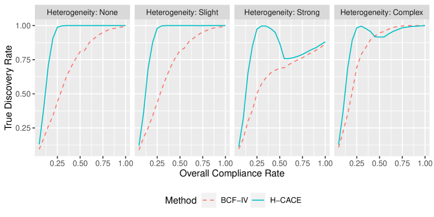
Figure 1 shows the true discovery rate under four treatment heterogeneity settings. We see that as the compliance rate (i.e. instrument strength) increases, the true discovery rate of our method grows across all settings. In particular, our approach has the best power in the region where the compliance rate is low, roughly under 40%. Even when the compliance rate is high, we see that BCF-IV generally has lower power than our method across different heterogeneity settings.
We also take a moment to explain a counter-intuitive dip in our method’s true discovery rate under the strong and complex heterogeneity settings in Figure 1. Briefly, this drop in the true discovery rate is due to the formation of leaves with smaller treatment effects. As the compliance rate becomes large, these small effects begin to be get suggested by CART. But, the power to reject the null in favor of these small effects are small and the overall true discovery rate dips briefly. However, as the compliance rate reaches one, we see the true discovery rate of our method begin to climb again. Web Appendix E contains additional details surrounding this phenomena.
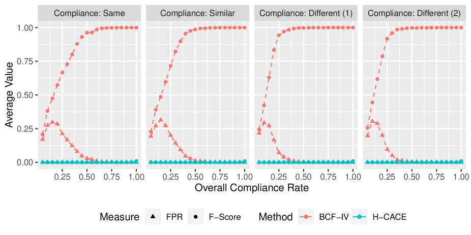
3.2 False Positive Rate and F-Score
We also assess our algorithm’s ability to select variables among that are true effect modifiers. Specifically, we define a true effect modifier as a variable among where the tree splits on the variable and rejects one of the hypotheses of the split’s children. A false effect modifier is a variable where the tree either does not split on the variable or fails to reject on one of the hypotheses defined by the variable. Using this definition, we use the F-score and the false positive rate (FPR) common in the classification literature to measure a method’s ability to select true effect modifiers. The F-score is the harmonic mean of recall and precision, where precision is the number of true positives (i.e. correctly selected true effect modifiers) out of the positive predictions (i.e. variables selected to be effect modifiers) and recall is the number of true positives out of the true conditions (i.e. true effect modifiers). More precisely, the F-score can be rewritten in terms of true positives (TP), false positives (FP), and false negatives (FN).
The F-score ranges from zero to one with a value closer to one implying greater accuracy. The FPR is defined as the number of false positives (i.e. incorrectly selected as a true effect modifier) out of the negative conditions (i.e. false effect modifiers) and ranges from zero to one, with a value close to zero being preferred.
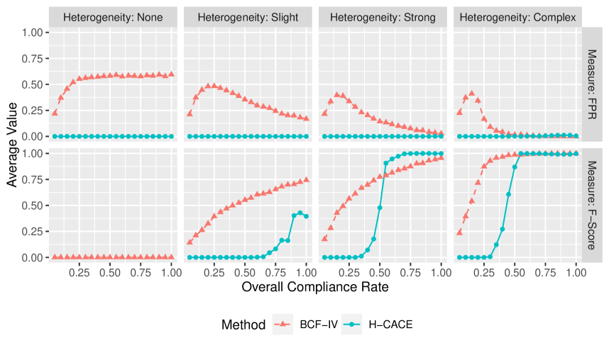
We use the same four heterogeneity settings of (a) No Heterogeneity, (b) Slight Heterogeneity, (c) Strong Heterogeneity, and (d) Complex Heterogeneity. Figure 2 shows the results of the F-score and FPR of our proposed algorithm and BCF-IV. Across four settings, our proposal has a false positive rate of nearly zero, never falsely declaring a variable to be a true effect modifier when it isn’t in reality. In contrast, BCF-IV has a larger false positive rate, declaring effect modifiers to be true effect modifiers even if they are actually false effect modifiers. For example, in setting (a) without any effect modifiers, BCF-IV has a false positive rate hovering above 50% whereas our method has a false positive rate of 0%. In other words, BCF-IV falsely declared at least one of the six covariates as true effect modifiers roughly 50% of the time whereas our method never declared any of the six covariates as true effect modifiers.
However, our algorithm’s F-score is generally smaller than that from BCF-IV unless the compliance rate is high and the effect heterogeneity is strong. In particular, when the compliance rate is roughly under 50% or if two subgroups have similar effect sizes, our method cannot select the true effect modifiers as well as BCF-IV. But, when the compliance rate is above 50% and the effect heterogeneity is strong, our algorithm has similar F-scores as BCF-IV. Overall, the low F-score is a price that our algorithm pays for making sure that the FPR is small. In contrast, BCF-IV has a higher F-score, but pays a price with a high FPR.
In the supplementary materials Web Appendix C, D, and F, we conduct additional simulation studies where we (i) vary the compliance rate by covariates, (ii) allow H-CACEs to be equal in magnitude, but opposite in direction to measure the effect of using in our algorithm, and (iii) demonstrate the two methods in a simulation that closely resembles the data from the OHIE. To summarize the results, for (i) and (iii), the story is very similar to what’s presented here, where our method has high true discovery rate, low FPR and F-score compared to those from BCF-IV. For (ii), as expected, we find that our method has a low true discovery rate, FPR, and F-score. But, as soon as the magnitudes of the H-CACEs are dissimilar, our method returns to the case presented here.
3.3 Takeaways from the Simulation Study
Overall, the simulation study shows that our algorithm has large statistical power and low false positive rate across all settings. In contrast, the BCF-IV algorithm had low power and produced large FPRs, especially when no effect heterogeneity exists in the data; in other words, BCF-IV often falsely declared an effect modifier to be true effect modifiers. But, our algorithm generally had a low F-score compared to that from BCF-IV except in regimes where the effect heterogeneity is strong and the compliance rate is high. Clearly, no one method uniformly dominates the other in every data generating model under every metric of performance. Instead, we hope the simulation study here alerts investigators about the strengths and limitations of our algorithm compared to existing approaches.
We also remark that the simulation results in Sections 3.1 and 3.2 do not necessarily contradict each other. Roughly speaking, the result in Section 3.1 concerns the ability for algorithms to have high statistical power whereas the result in Section 3.2 concerns the ability for algorithms to select variables. An algorithm like BCF-IV could liberally select many effect modifiers, generally leading to a high F-score and potentially a high FPR. But, the power to test the nulls suggested by the selected effect modifiers could be low since not only may some of these selected variables not be true effect modifiers, but also the selected variables will define many subgroups which likely contain few units to test the corresponding nulls. In contrast, an algorithm like ours could conservatively select effect modifiers, leading to a small F-score and low FPR. But, the power to test the nulls suggested by the selected variables could be high since most of the selected variables will be true effect modifiers. In short, our method is somewhat cautious, but certain whereas BCF-IV is optimistic, but somewhat error-prone.
4 Analysis of the Oregon Health Insurance Experiment
4.1 Data Description
We use our method to analyze the heterogeneous effects of Medicaid on the number of days an individual’s physical or mental health prevented their usual activities in the past month. In brief, the OHIE collected administrative data on hospital discharges, credit reports, and mortality, survey data on health care utilization, financial strain, and overall health, and pre-randomization demographic data. There were 11,808 lottery winners and 11,933 lottery losers in the publicly available survey data for a total sample size of 23,741 individuals; see Finkelstein et al., (2012) for details.
We matched on the following demographic, pre-randomization variables recorded by Finkelstein et al., (2012): sex, age, whether they preferred English materials when signing up for the lottery, whether they lived in a metropolitan statistical area (MSA), their education level (less than high school, high school diploma or General Educational Development (GED), vocational or 2-year degree, 4-year college degree or more), and self-identified race (as the individual reported in the survey). Since some of the covariates had missing data, namely self-identifying as Hispanic or Black and their level of education, we also matched on indicators of their missingness; see Section 9.4 of Rosenbaum, (2010) for details. We used the R package bigmatch, version 0.6.1, (Yu,, 2019) with an optimal caliper and a robust rank-based Mahalanobis distance to generate our optimal pair match. Figure 3 shows covariate balance before and after matching.
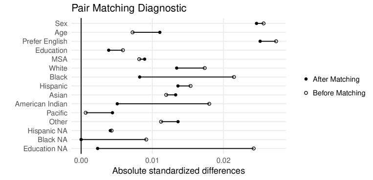
For the majority of covariates, the matching algorithm did little to change the absolute standard differences between lottery winners and losers. This is not surprising given that the lottery was randomized. However, the indicator for missingness in education, self-identified American Indian, and Black were made to be more similar after matching. An absolute standardized difference of 0.25 is deemed acceptable (Rubin,, 2001, Stuart,, 2010), which our covariates satisfied after matching.
4.2 Instrument Validity
Before we present the results of our analysis using the proposed method, we discuss the plausibility of the lottery as an instrument. The lottery is randomized which ensures that the instrument is unrelated to unmeasured confounders and satisfying (A3). Winning the lottery, on average, increased enrollment of Medicaid by 30% (Finkelstein et al.,, 2012), satisfying (A1). Assumption (A4) in the context of the OHIE states that there are no individuals who defy the lottery assignment to take (or not take) Medicaid if they lost (or won) the lottery. This is guaranteed by the design of the lottery, since an individual who lost the lottery cannot have access to Medicaid. However, we remark that Finkelstein et al., (2012) measured the treatment as whether or not an individual has ever had Medicaid during the study and a few individuals were already enrolled in Medicaid before the lottery winners were announced. Finally, assumption (A2) is the only assumption that could potentially be violated since individuals were not blind to their lottery results. This theoretically allowed lottery losers to seek other health insurance or lottery winners to make less healthy decisions since they’re now able to be insured. These changes in an individual’s behavior could affect his/her outcome regardless of his/her treatment and thus, may violate (A2).
4.3 Analysis and Results
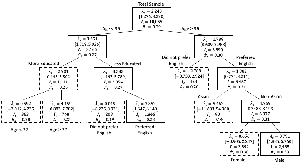
We run Algorithm 1 and present the results in Figure 4. We remark that we used rpart in R with a complexity parameter of 0 and maximum depth of 4. The depth of the tree was chosen by forming trees of larger depth and then pruning back until a more interpretable tree was obtained. For each node of the CART, we tested whether or not there is an effect of enrolling in Medicaid . In Figure 4, a solid lined box denotes a null hypothesis that was rejected and a dashed lined box denotes a null hypothesis that was retained, both by the closed testing procedure. Each node contains its estimated H-CACE , 95% confidence interval, the number of pairs , and the estimated compliance rate . Here, a positive H-CACE implies a decrease in the number of days where the individual’s physical and mental health prevented them from their usual activities, and a negative value implies an increase; in short, positive effects are beneficial to individuals. Also, some nodes imply a significant effect of Medicaid at level 0.05, but are enclosed in a dashed lined box. This is due to the closed testing procedure; an intersection of hypotheses containing the node in question was not rejected, and so any hypotheses in this intersection could not be rejected.
From Figure 4, we can see evidence of heterogeneous treatment effects among the complier population. Specifically, Medicaid had a strong effect (1) among complying non-Asian men over the age of 36 and who prefer English, as well as (2) complying individuals younger than 36, who prefer English, and does not have more than a high school diploma or GED. Interestingly, among non-Asians over the age of 36 and who prefer English, females did not benefit from Medicaid as much as males even though the female subgroup was larger than the male subgroup and the compliance rates between the two subgroups were similar.
More generally, while there is some variation in the compliance rates between groups, most of them are minor and hover between 25% to 30%. The minor variation suggests that while some subgroups are more likely to be compliers than others, most of the effect heterogeneity is likely driven by the variation in how the treatment differentially changes the response across subgroups; a bit more formally, most of the effect heterogeneity is likely arising from the numerator of the H-CACE rather than the denominator of the H-CACE.
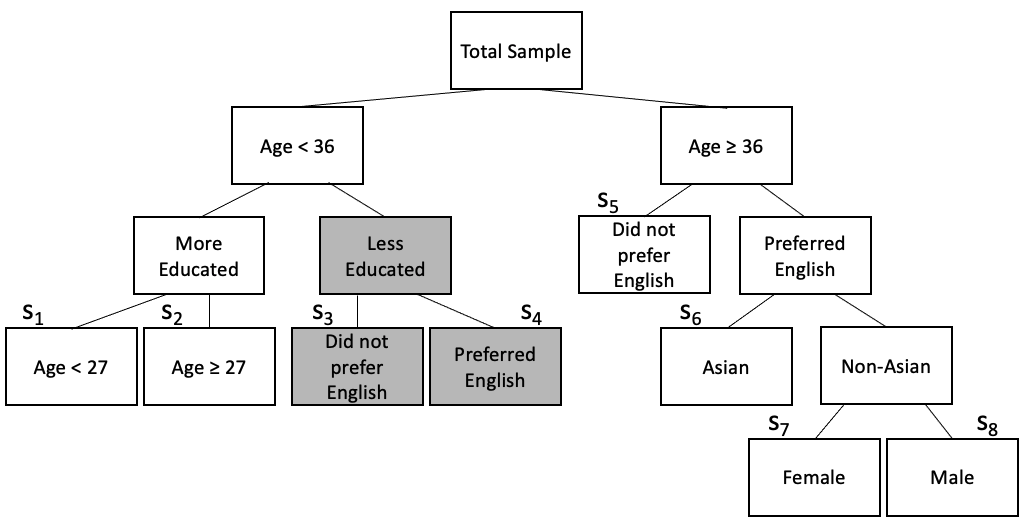
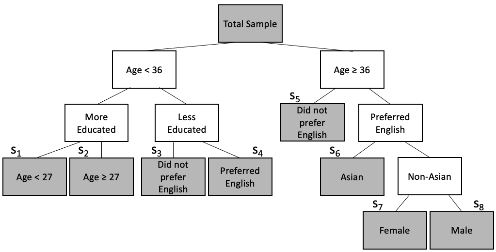
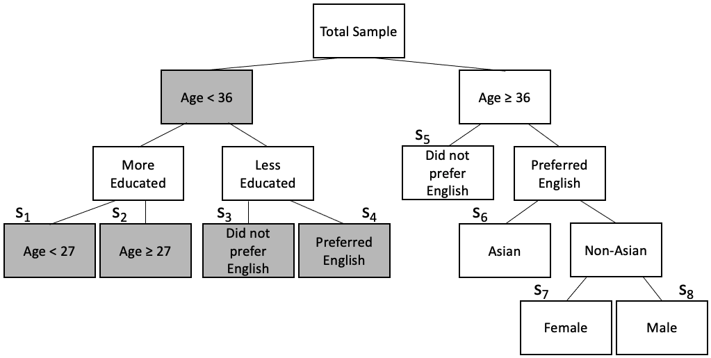
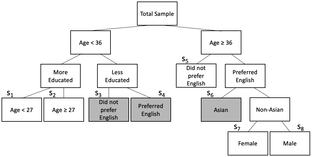
4.4 An Example of Closed Testing
To better illustrate the closed testing portion of Algorithm 1, we walk through an example of the testing procedure based on the OHIE. As seen in Figure 4, CART produced a tree with leaves. Now, consider testing whether there is evidence of a heterogeneous effect of Medicaid for young individuals who prefer English and have at most a high school diploma or GED, i.e. node in Figure 5 and using Algorithm 1’s notation. The null hypothesis of interest would be , for all and . We then test and reject all of the hypothesis tests containing group . For example, we need to test the null hypothesis concerning the ancestor of , say the subgroup of individuals who are younger than 36 and have at most a high school diploma or GED denoted as ; see part (a) of Figure 5. Additionally, we need to test and reject all of the supersets containing , which include but are not limited to the overall set , , and . If every superset hypothesis and are rejected at level , we can declare the effect in node to be significant and, by Proposition 1, the familywise error rate is controlled at . Repeating this process for every node in the tree will give the results in Figure 4.
5 Discussion
In this paper, we propose a method based on matching to detect effect heterogeneity using an instrument. Under the usual IV assumptions, our method discovers and tests heterogeneity in the complier average treatment effect by combining matching, CART, and closed testing, all without the need to do sample splitting. The latter is achieved by taking the absolute value of the adjusted pairwise differences to conceal the instrument assignment and this allows our proposed method to control the familywise error rate. We also conducted a simulation study to examine the performance of our method and compared it to a recent method referred to as BCF-IV. Our method was then used to study the effect of Medicaid on the number of days an individual’s physical or mental health did not prevent their usual activities where we used the lottery selection as an instrument. We found that Medicaid benefitted complying, older, non-Asian men who selected English materials at lottery sign-up and for complying, younger, less educated individuals who selected English materials at lottery sign-up.
We conclude by making some recommendations about how to properly use our algorithm in practice, especially in light of existing approaches. First, as explained in the introduction, when there is noncompliance, exploring heterogeneity in the ITT alone with existing methods may provide an incomplete picture of the nature of the treatment effect. Relatedly, in settings where unmeasured confounding is unavoidable, our method based on an instrument is a promising way to discover and test effect heterogeneity.
Second, as alluded to in Section 3.3, the simulation results suggest that our algorithm tends to be conservative in discovering novel effect modifiers, reporting mostly true effect modifiers only if there is strong evidence for heterogeneity and minimizing selection of false effect modifiers. In other words, investigators can be reasonably confident that effect heterogeneity exists among the variables declared by our algorithm as effect modifiers. But, those variables that are not selected by our algorithm may also be true effect modifiers, but with slight effect heterogeneity. In such cases, investigators may need additional samples to detect them using our method. In contrast, BCF-IV tends to be anti-conservative, reporting more effect modifiers, some of which may not actually be true effect modifiers. While this may be advantageous in situations where there is slight effect heterogeneity, investigators may not feel as confident about whether the detected effect heterogeneity truly exists.
Third, most recent approaches on effect heterogeneity, notably Chernozhukov et al., (2018), utilize sample splitting to achieve honest inference (i.e. type I error rate control) whereas our method uses absolute value of matched pairs to achieve it; note that both methods theoretically allow for a large class of machine learning methods to detect heterogeneous treatment effects, even though ours focused on CART for its simplicity and interpretability. While our method uses the full sample for both discovery and honest testing compared to those based on sample splitting, one of the caveats of our method is that our method may not be able to detect subgroups with identical effect sizes, but in opposite signs. Overall, every algorithm for effect heterogeneity carries some trade-offs and we urge investigators to understand their strengths and limitations to solidify and strengthen causal conclusions about effect heterogeneity in IV studies.
Web Appendix A
Honest Simultaneous Discovery and Inference
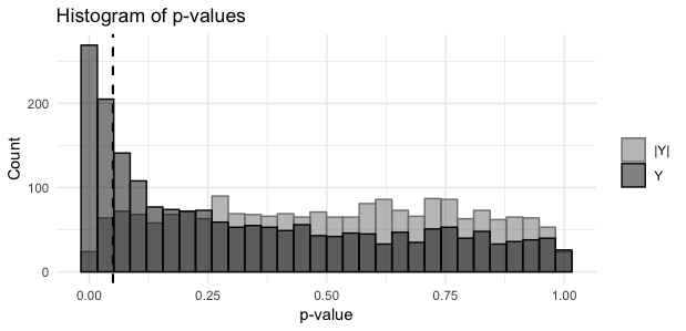
One advantage of our method is being able to use the entire data for discovering and testing effect modifiers. In order to simultaneously discover and draw inference on the sample, we use the absolute value of the pairwise differences as the outcome of CART to obscure the sign of the difference in adjusted outcomes and preserve the original distribution of the instrumental variables (i.e. distribution based on assumption (A3)). We can then use this distribution to draw inference on our discovered potential effect modifiers. We study this phenomenon in two cases: (1) testing a single effect modifier (i.e. one hypothesis) and (2) testing multiple effect modifiers (i.e. multiple hypothesis).
In the first case, we are concerned about testing a single hypothesis and controlling the Type I error rate after discovering the hypothesis via CART. To investigate the effect of simultaneously discovering and drawing inference, we generate the potential outcomes with no treatment effect, for all , and form potential effect modifiers for two different cases, (i) using and (ii) as the outcome for CART. The first leaf of each tree (or tree’s root if no leaves are formed) is then used to test the null hypothesis of no treatment effect. As a result of conducting CART to form a hypothesis 2000 times, Figure 6 shows the histogram of -values when we use as the outcome for CART versus as the outcome for CART. Under , the -values resemble a uniform distribution and hence, Type I error is controlled. However, under , the -values are right-skewed implying that Type I error is inflated. In other words, the null hypothesis is rejected more frequently when using as the outcome of CART, demonstrating the “winner’s curse” phenomena. Therefore, as predicted by Proposition 1, using as the outcome in CART prevents the contamination of the level of the hypothesis test and allow for simultaneous discovery and inference.
In the second case, with multiple hypotheses, we are concerned with the average Type I error rate and strong control of the familywise error rate rate when testing multiple hypotheses. To evaluate strong control of the familywise error rate, we generate the data where there is an effect in some groups and no effect in others, , . Furthermore, for rpart, we reduce the complexity parameter to 0.0001 to encourage more liberal splitting and set the max depth of the regression tree to be 4 to save on computational time. After data generation we randomly assign instrument values within pairs and split the data using and 2000 times. Each hypothesis is tested for whether or not there is a treatment effect , so true hypotheses are hypotheses of groups of pairs generated with . The average Type I error rate is computed by taking the average of the proportion of false rejections from each of the 2000 simulated trees and the familywise error rate is computed by taking the average of any false rejections amongst the 2000 simulated trees.
| Simulation Setting | Mean Type I error rate | Familywise error rate |
|---|---|---|
| 0.0008 | 0.028 | |
| 0.0003 | 0.028 |
The results of this simulation show that the average type I error rate and familywise error rate are below the level of the hypothesis tests in both simulation settings and . The average Type I error rate for and is 0.0008 and 0.0003, respectively. The familywise error rate for both and is 0.028 (See Table 1). This is surprising considering that closed testing requires that each hypothesis test be level to strongly control the familywise error rate and using as the outcome contaminates the test’s level. Despite the theoretical underpinnings for this data generation process, closed testing seems to strongly control the familywise error rate regardless of whether or not the test’s size is preserved by a technique such as taking the absolute value. Upon closer investigation, it seems that the trees formed in both and cases are the same at the upper levels of the tree, as there is a particularly strong signal for a certain group . This then leads to the same hypotheses in both settings resulting in similar Type I error rates and familywise error rates. Overall, the simulation suggests that in the case where there is one very strong signal, the difference between using and is minor. But, we do stress familywise error control is only guaranteed for the case.
Web Appendix B
Proposition 1 (Familywise Error Rate Control of Algorithm 1).
Under the sharp null hypotheses in Algorithm 1, the conditional probability given that the algorithm makes at least one false rejection of the set of hypotheses is at most .
Proof.
Define to be the union of all groups of pairs for which the null hypothesis is true; the groups of pairs of individuals which have an effect ratio of . In order to have a notion of type I error, some hypothesis or hypotheses must be true, so we assume that and that hypothesis for is true. Note that by definition of , in order for to be true, the groups in are also contained in , . To make a type I error and reject hypothesis , Algorithm 2 must reject the intersection of all true hypotheses , where and . Yet, rejecting requires , where . Therefore, to make a type I error and reject , one must reject which is a level test. ∎
Web Appendix C
Detecting H-CACE under Varying Compliance
In section 3, the simulation settings assumed constant compliance rates across the groups. But it is possible that the compliance rates vary between subgroups. Therefore, we further consider four varying compliance rate settings as an extension of understanding the method’s performance. These four different compliance settings are referred to as (a) Same, (b) Similar, (c) Different (1), and (d) Different (2) and are functions of the overall compliance rate . Each are categorized based on the distance from the overall compliance rate. If the overall compliance is less than a half, , a group’s compliance rate is , and if , a group’s compliance rate is for some constant . The four settings are then defined by the constants ; (a) Same compliance: ; (b) Similar compliance: and ; (c) Different (1) compliance: and ; and Different (2) compliance: , , , and . When combined with the treatment heterogeneity settings, we have a total of 16 possible settings of heterogeneity in H-CACE. We also remark that subgroups experiencing a larger H-CACE have a small compliance rate. Again, we compare our method to the BCF-IV method (Bargagli-Stoffi et al.,, 2019).
Figure 7 shows the true discovery rate of the four compliance types for each treatment heterogeneity setting. As in Section 3, this is a measure of the statistical power, where the true discovery rate is defined as the number of false hypotheses rejected out of all false hypotheses tested by closed testing. The different facets denote the treatment effect heterogeneity and the compliance heterogeneity. As the compliance rates get more different, we observe a reduction in the true discovery rate. This is most noticeable in the strong heterogeneity setting, where we see pronounced differences in the true discovery rate among the different compliance settings. In this setting, we also see a change in the true discovery rate between the more different (Different (1) and (2)) and more similar (Same and Similar) compliance groups; the more different compliance groups have an increased true discovery rate after an overall compliance rate of . This is due to the low compliance rate in the groups with stronger H-CACE in Different (1) and Different (2) settings, obscuring the signal for which CART uses to define subgroups. Therefore, the dip described in Section 3 and explained in Web Appendix E that is observed in the Strong Heterogeneous and Same Compliance settings (Figure 7) occurs at a high overall compliance rate for the Different (1) and Different (2) settings. In the heterogeneity settings, as the overall compliance rate grows, so too does the subgroup-specific compliance rates, and so the true discovery rates of the compliance settings converge. This is evidence that our method’s true discovery rate relies on both the subgroup-specific size of H-CACEs and subgroup-specific compliance rates.
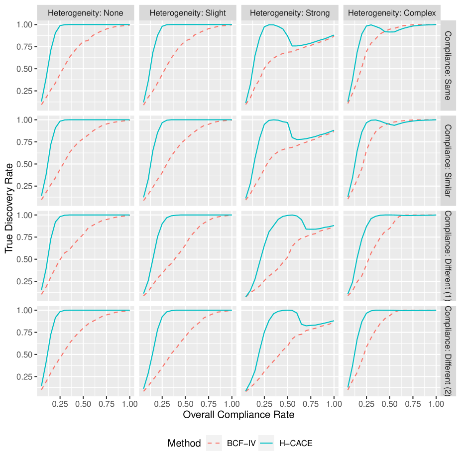
Figure 8 shows the F-score and false positive rate (FPR) of the four compliance types for each treatment heterogeneity setting. As in Section 3, these are binary classification measures evaluating the algorithms’ ability to detect true and false effect modification. For true positives (TP), false positives (FP), and false negatives (FN), the F-score is defined to be , and the FPR is defined as the number of false positives out of the negative conditions. Similarly to Figure 7, as the compliance rates get more different, we observe a reduction in the performance of the algorithms. This is most noticeable in the Slight and Strong Heterogeneity settings for the BCF-IV algorithm and in the Strong and Complex Heterogeneity settings for our proposed algorithm. For the BCF-IV algorithm, the FPR begins to decline at a larger overall compliance rate in the more heterogeneous compliance settings, and the F-score of our algorithm climbs at a later overall compliance rate as well. As was the case with the true discovery rate, this is evidence that the FPR and F-score rely on both the H-CACE and compliance rate heterogeneity.
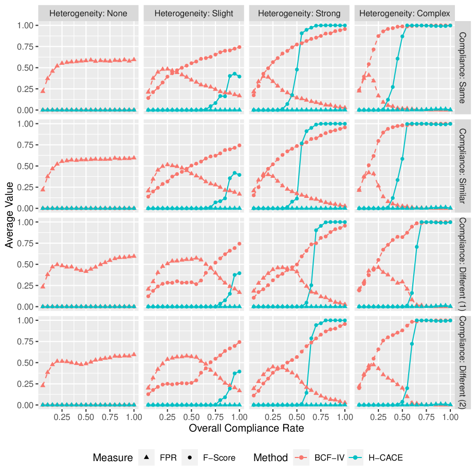
These simulations are evidence that our method’s ability, as measured in statistical power and selection of effect modifiers relies on both the subgroup-specific size of H-CACEs and the subgroup-specific compliance rates.
Web Appendix D
Testing for Equal, But Opposite Effects
As it is possible that H-CACEs are equal in magnitude but opposite in direction, it is a question of how our method performs when we take the absolute value of the pairwise differences. To evaluate our method in this specific situation, we generate data as described in Section 3 but now considering only the heterogeneity setting , and . Now, there are two effect modifiers and where changes the magnitude of the H-CACE and changes the direction. We compare our method to the BCF-IV method (Bargagli-Stoffi et al.,, 2019) as it does not transform the outcome and should still be able to detect the effect modification in this setting.
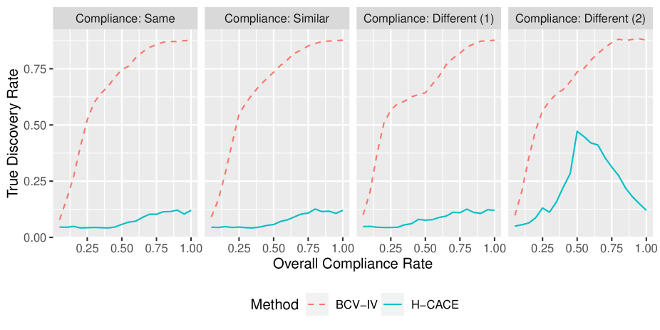
In Figures 9 and 10, we see our method underperform in detecting heterogeneous treatment effects in this setting of equal but opposite effects, both in true discovery rate and F-score. The reason is two fold. First, in the transformation of the outcome of CART, the absolute value of the pairwise differences obscures the signal and hinders CART’s ability to properly split. Second, in the case that CART does split, our closed testing procedure makes it challenging to reject the hypotheses suggested, since we must first reject the global hypothesis of . As we point out in Section 2.3, the CACE is a weighted average of the H-CACEs in the global test, and it is therefore unlikely to reject as the average of the H-CACEs is 0. Together, CART’s inability to split and the global hypothesis needing to be first rejected, our proposed method underperforms in the setting with equal but opposite effects. We therefore express caution in using our algorithm in the occasion an investigator believes the effect sizes are equal but opposite.
Interestingly, we see a spike of increased true discovery rate for both methods in the Different (2) compliance setting. In this setting, the compliance rates for the four groups are , , , and when the overall compliance rate is less than or equal to 0.5, and , , , and when . Therefore, when is close to 0.5, the compliance rates are approach , , , and for the four groups, changing the weights of the H-CACEs in the average for the global effect and shifting its value away from 0. As the overall compliance approaches 0 or 1, the heterogeneity in the compliance of the four groups reduces so the average of the H-CACEs approaches 0. This all improves our statistical test’s ability to reject the global hypothesis and increase the true discovery rate. We do not see a large improvement however, as CART still fails to split. We note that in the case that the magnitudes are unequal, then our method will return to the performance demonstrated in Section 3, as CART will have signal to split on and our global hypothesis will more easily be correctly rejected. This can be seen in an example that the heterogeneity has the form , and the dotted line represents pairs from . With the absolute value transformation of the pairwise differences, our algorithm would treat this setting as in the Strong Heterogeneity setting we simulate in Section 3.
Web Appendix E
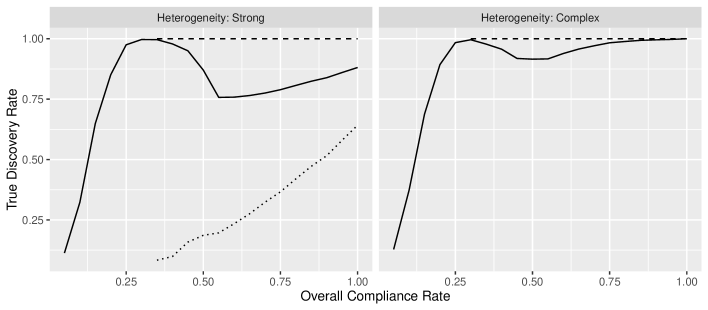
Counter-intuitive Dip in True Discovery Rate
As mentioned in Section 3 and shown in Figure 11, we observe a counter-intuitive dip in true discovery rate as compliance rate grows for our proposed method. To investigate this drop, we also plot in different line types the true discovery rate of single subgroups formed by CART. The dashed lines denote leaves containing pairs with a stronger treatment effect and the dotted lines denote leaves containing pairs with a weaker treatment effect. For example, in the strong heterogeneity setting, the dashed line represents pairs from , and the dotted line represents pairs from . For the complex heterogeneity setting, the dashed line denotes pairs generated by ; dotted lines aren’t shown because CART fails to form a group consisting of only pairs generated by . By comparing the curves, we see that as the compliance rate grows the drop in the true discovery rate is due to the formation of leaves with smaller treatment effects. Because the compliance rate is large enough, these small effects are beginning to be detected by CART. But, the power to detect these effects are much smaller than the large effects, and so the overall true discovery rate, which is roughly the average of these two curves, dips briefly. However, As the compliance rate grows, we see the true discovery rate of our method begin to climb again, as more signal for the smaller H-CACE groups is gained.
Web Appendix F
Oregon Health Insurance Experiment Simulation
Using the Oregon Health Insurance Experiment (OHIE) as a template for another simulation, we evaluate the performance of the proposed method under treatment magnitudes using the true discovery rate as a measure of the method’s statistical power, and false positive rate (FPR) and F-score to measure the method’s performance in determining effect modifiers. Using the matched pairs from the OHIE and their pre-instrument covariates , we generate the potential treatments and and potential outcomes and . Since the design of the OHIE ensures one-sided compliance, we generate the potential treatment without receiving the outcome to also satisfy one-sided compliance, . To have similar compliance rates as observed in Section 4, the potential treatment having received the instrument is a Bernoulli trial with success rate . Here, is a binary indicator where a value of denotes the individual’s preference for English materials in signing up for the lottery, and is a binary indicator where a value of denotes the race reported in the survey as Asian. With this heterogeneous compliance rate, the overall compliance is the same as that estimated for the sample in Section 4, . We then generate the potential outcomes as in Section 3, the potential outcomes having not received the instrument are from a standard normal distribution , and the potential outcomes having received the instrument are a function of the H-CACE and effect modifiers detected in Section 4, . The H-CACE is a function of the effect modifiers , , , , and and the magnitude of the effects are defined in three settings:
-
(i)
Small:
-
(ii)
Moderate:
-
(iii)
Large:
As in Section 4, is a binary variable where a value of 1 denotes a vocational degree, 2-year degree, 4-year college degree, or more.
For our proposed method, we use the R package rpart with a complexity parameter of 0.001, max depth of 7, and minimum number of observations needed for a split to be 90. This allows CART to split on more variables than the number of effect modifiers while preventing the creation of nodes with very few observations. For BCF-IV, we use the default rpart settings as in Section 3. The averages of the 1000 simulations at each treatment magnitude level are provided in Table 2.
The results of this simulation are similar to those seen in Section 3, where our proposed method performs well in the true discovery rate, but performs poorly in the FPR and F-score when the compliance rate is low and the heterogeneity magnitudes are weak. This further aligns with our results in Section 3, as we found our method struggles selecting effect modifiers as measured by the F-score at compliance rates below 50% and the compliance rate is 29% in this setting. However, we see that our method improves in the F-score as the treatment magnitude increases. In contrast, BCF-IV outperforms our method in the F-score, but has an inflated FPR and a deflated true discovery rate. However, as the signal improves, BCF-IV’s FPR reduces to a more ideal value and the true discovery rate grows.
| Method | True Discovery Rate | FPR | F-Score | |
|---|---|---|---|---|
| H-CACE | Small | 1.00 | 0.00 | 0.00 |
| Moderate | 0.99 | 0.02 | 0.04 | |
| Large | 0.99 | 0.06 | 0.76 | |
| BCF-IV | Small | 0.72 | 0.17 | 0.56 |
| Moderate | 0.83 | 0.05 | 0.74 | |
| Large | 0.93 | 0.01 | 0.88 |
References
- Abadie, (2003) Abadie, A. (2003). Semiparametric instrumental variable estimation of treatment response models. Journal of Econometrics, 113(2):231–263.
- Ai and Chen, (2003) Ai, C. and Chen, X. (2003). Efficient estimation of models with conditional moment restrictions containing unknown functions. Econometrica, 71(6):1795–1843.
- Angrist et al., (1996) Angrist, J. D., Imbens, G. W., and Rubin, D. B. (1996). Identification of causal effects using instrumental variables. Journal of the American Statistical Association, 91(434):444–455.
- Athey and Imbens, (2016) Athey, S. and Imbens, G. (2016). Recursive partitioning for heterogeneous causal effects. Proceedings of the National Academy of Sciences, 113(27):7353–7360.
- Athey and Imbens, (2015) Athey, S. and Imbens, G. W. (2015). Machine learning methods for estimating heterogeneous causal effects. arXiv:1504.01132v1 [stat.ML].
- Athey et al., (2019) Athey, S., Tibshirani, J., Wager, S., et al. (2019). Generalized random forests. The Annals of Statistics, 47(2):1148–1178.
- Baiocchi et al., (2014) Baiocchi, M., Cheng, J., and Small, D. S. (2014). Instrumental variable methods for causal inference. Statistics in Medicine, 33(13):2297–2340.
- Baiocchi et al., (2010) Baiocchi, M., Small, D. S., Lorch, S., and Rosenbaum, P. R. (2010). Building a stronger instrument in an observational study of perinatal care for premature infants. Journal of the American Statistical Association, 105(492):1285–1296.
- Balke and Pearl, (1997) Balke, A. and Pearl, J. (1997). Bounds on treatment effects from studies with imperfect compliance. Journal of the American Statistical Association, 92(439):1171–1176.
- Bargagli-Stoffi et al., (2019) Bargagli-Stoffi, F. J., De-Witte, K., and Gnecco, G. (2019). Heterogeneous causal effects with imperfect compliance: a novel bayesian machine learning approach. arXiv:1905.12707 [stat.ME].
- Bargagli-Stoffi and Gnecco, (2018) Bargagli-Stoffi, F. J. and Gnecco, G. (2018). Estimating heterogeneous causal effects in the presence of irregular assignment mechanisms. In 2018 IEEE 5th International Conference on Data Science and Advanced Analytics (DSAA), pages 1–10. IEEE.
- Blundell et al., (2007) Blundell, R., Chen, X., and Kristensen, D. (2007). Semi-nonparametric iv estimation of shape-invariant engel curves. Econometrica, 75(6):1613–1669.
- Blundell and Powell, (2003) Blundell, R. and Powell, J. L. (2003). Endogeneity in nonparametric and semiparametric regression models. Econometric Society Monographs, 36:312–357.
- Breiman et al., (1984) Breiman, L., Friedman, J., Olshen, R., and Stone, C. (1984). Classification and Regression Trees. New York: Chapman and Hall/CRC.
- Chen and Pouzo, (2012) Chen, X. and Pouzo, D. (2012). Estimation of nonparametric conditional moment models with possibly nonsmooth generalized residuals. Econometrica, 80(1):277–321.
- Chernozhukov et al., (2018) Chernozhukov, V., Demirer, M., Duflo, E., and Fernandez-Val, I. (2018). Generic machine learning inference on heterogenous treatment effects in randomized experiments. National Bureau of Economic Research.
- Darolles et al., (2011) Darolles, S., Fan, Y., Florens, J.-P., and Renault, E. (2011). Nonparametric instrumental regression. Econometrica, 79(5):1541–1565.
- Ding, (2017) Ding, P. (2017). A paradox from randomization-based causal inference. Statistical Science, 32(3):331–345.
- Finkelstein et al., (2012) Finkelstein, A., Taubman, S., Wright, B., Bernstein, M., Gruber, J., Newhouse, J. P., Allen, H., Baicker, K., and Group, O. H. S. (2012). The oregon health insurance experiment: evidence from the first year. The Quarterly Journal of Economics, 127(3):1057–1106.
- Fogarty, (2018) Fogarty, C. B. (2018). Regression-assisted inference for the average treatment effect in paired experiments. Biometrika, 105(4):994–1000.
- Fogarty, (2020) Fogarty, C. B. (2020). Studentized sensitivity analysis for the sample average treatment effect in paired observational studies. Journal of the American Statistical Association, 115(531):1518–1530.
- Fogarty et al., (2020) Fogarty, C. B., Lee, K., Kelz, R. R., and Keele, L. J. (2020). Biased encouragements and heterogeneous effects in an instrumental variable study of emergency general surgical outcomes. Journal of the American Statistical Association, pages 1–32.
- Hahn et al., (2017) Hahn, P. R., Murray, J. S., and Carvalho, C. (2017). Bayesian regression tree models for causal inference: regularization, confounding, and heterogeneous effects. arXiv:1706.09523 [stat,ME].
- Hall and Horowitz, (2005) Hall, P. and Horowitz, J. L. (2005). Nonparametric methods for inference in the presence of instrumental variables. The Annals of Statistics, 33(6):2904–2929.
- Hernán and Robins, (2006) Hernán, M. A. and Robins, J. M. (2006). Instruments for causal inference: an epidemiologist’s dream? Epidemiology, 17(4):360–372.
- Hill, (2011) Hill, J. L. (2011). Bayesian nonparametric modeling for causal inference. Journal of Computational and Graphical Statistics, 20(1):217–240.
- Hodges and Lehmann, (1963) Hodges, J. L. and Lehmann, E. L. (1963). Estimates of location based on rank tests. The Annals of Mathematical Statistics, 34(2):598–611.
- Hsu et al., (2013) Hsu, J. Y., Small, D. S., and Rosenbaum, P. R. (2013). Effect modification and design sensitivity in observational studies. Journal of the American Statistical Association, 108(501):135–148.
- Hsu et al., (2015) Hsu, J. Y., Zubizarreta, J. R., Small, D. S., and Rosenbaum, P. R. (2015). Strong control of the familywise error rate in observational studies that discover effect modification by exploratory methods. Biometrika, 102(4):767–782.
- Imbens, (2010) Imbens, G. W. (2010). Better late than nothing: Some comments on deaton (2009) and heckman and urzua (2009). Journal of Economic Literature, 48(2):399–423.
- Kang et al., (2013) Kang, H., Kreuels, B., Adjei, O., Krumkamp, R., May, J., and Small, D. S. (2013). The causal effect of malaria on stunting: a mendelian randomization and matching approach. International Journal of Epidemiology, 42(5):1390–1398.
- Kang et al., (2016) Kang, H., Kreuels, B., May, J., Small, D. S., et al. (2016). Full matching approach to instrumental variables estimation with application to the effect of malaria on stunting. The Annals of Applied Statistics, 10(1):335–364.
- Kang et al., (2018) Kang, H., Peck, L., and Keele, L. (2018). Inference for instrumental variables: a randomization inference approach. Journal of the Royal Statistical Society: Series A (Statistics in Society), 181(4):1231–1254.
- (34) Lee, K., Small, D. S., and Dominici, F. (2018a). Discovering effect modification and randomization inference in air pollution studies. arXiv:1802.06710 [stat.AP].
- (35) Lee, K., Small, D. S., Hsu, J. Y., Silber, J. H., and Rosenbaum, P. R. (2018b). Discovering effect modification in an observational study of surgical mortality at hospitals with superior nursing. Journal of the Royal Statistical Society: Series A (Statistics in Society), 181(2):535–546.
- (36) Lee, K., Small, D. S., and Rosenbaum, P. R. (2018c). A powerful approach to the study of moderate effect modification in observational studies. Biometrics, 74(4):1161–1170.
- Marcus et al., (1976) Marcus, R., Eric, P., and Gabriel, K. R. (1976). On closed testing procedures with special reference to ordered analysis of variance. Biometrika, 63(3):655–660.
- Newey and Powell, (2003) Newey, W. K. and Powell, J. L. (2003). Instrumental variable estimation of nonparametric models. Econometrica, 71(5):1565–1578.
- Park and Kang, (2020) Park, C. and Kang, H. (2020). A groupwise approach for inferring heterogeneous treatment effects in causal inference. arXiv preprint arXiv:1908.04427v2.
- (40) Rosenbaum, P. R. (2002a). Covariance adjustment in randomized experiments and observational studies. Statistical Science, 17(3):286–327.
- (41) Rosenbaum, P. R. (2002b). [covariance adjustment in randomized experiments and observational studies]: Rejoinder. Statistical Science, 17(3):321–327.
- Rosenbaum, (2010) Rosenbaum, P. R. (2010). Design of Observational Studies. New York: Springer.
- Rosenbaum, (2020) Rosenbaum, P. R. (2020). Modern algorithms for matching in observational studies. Annual Review of Statistics and Its Application, 7:143–176.
- Rubin, (1980) Rubin, D. B. (1980). Randomization analysis of experimental data: The fisher randomization test comment. Journal of the American Statistical Association, 75(371):591–593.
- Rubin, (2001) Rubin, D. B. (2001). Using propensity scores to help design observational studies: application to the tobacco litigation. Health Services and Outcomes Research Methodology, 2(3-4):169–188.
- Staiger and Stock, (1997) Staiger, D. O. and Stock, J. H. (1997). Instrumental variables regression with weak instruments. Econometrica, 65(3):557–586.
- Stock et al., (2002) Stock, J. H., Wright, J. H., and Yogo, M. (2002). A survey of weak instruments and weak identification in generalized method of moments. Journal of Business & Economic Statistics, 20(4):518–529.
- Stuart, (2010) Stuart, E. A. (2010). Matching methods for causal inference: A review and a look forward. Statistical Science, 25(1):1–21.
- Su et al., (2013) Su, L., Murtazashvili, I., and Ullah, A. (2013). Local linear gmm estimation of functional coefficient iv models with an application to estimating the rate of return to schooling. Journal of Business & Economic Statistics, 31(2):184–207.
- Su et al., (2009) Su, X., Tsai, C.-L., Wang, H., Nickerson, D. M., and Li, B. (2009). Subgroup analysis via recursive partitioning. Journal of Machine Learning Research, 10:141–158.
- Swanson and Hernán, (2013) Swanson, S. A. and Hernán, M. A. (2013). Commentary: how to report instrumental variable analyses (suggestions welcome). Epidemiology, 24(3):370–374.
- Swanson and Hernán, (2014) Swanson, S. A. and Hernán, M. A. (2014). Think globally, act globally: an epidemiologist’s perspective on instrumental variable estimation. Statistical Science, 29(3):371–374.
- Therneau et al., (2015) Therneau, T., Atkinson, B., and Ripley, B. (2015). Package ‘rpart’. R package version 4.1-15. https://cran.r-project.org/package=rpart.
- Wager and Athey, (2018) Wager, S. and Athey, S. (2018). Estimation and inference of heterogeneous treatment effects using random forests. Journal of the American Statistical Association, 113(523):1228–1242.
- Yu, (2019) Yu, R. (2019). bigmatch: Making Optimal Matching Size-Scalable Using Optimal Calipers. R package version 0.6.1. https://CRAN.R-project.org/package=bigmatch.