The Chen-Teboulle algorithm is the proximal point algorithm

Abstract

We revisit the Chen-Teboulle algorithm using recent insights and show that this allows a better bound on the step-size parameter.

1 Background

Recent works such as [HY12] have proposed a very simple yet powerful technique for analyzing optimization methods. The idea consists simply of working with a different norm in the product Hilbert space. We fix an inner product $\langle x,y\rangle$ on $\mathcal{H}\times\mathcal{H}^{*}$. Instead of defining the norm to be the induced norm, we define the primal norm as follows (and this induces the dual norm)

$$\|x\|_{V}=\sqrt{\langle Vx,x\rangle}=\sqrt{\langle x,x\rangle_{V}},\quad\|y\|_{V}^{*}=\|y\|_{V^{-1}}=\sqrt{\langle y,V^{-1}y\rangle}=\sqrt{\langle y,y\rangle_{V^{-1}}}$$

for any Hermitian positive definite $V\in\mathcal{B}(\mathcal{H},\mathcal{H})$; we write this condition as $V\succ 0$. For finite dimensional spaces $\mathcal{H}$, this means that $V$ is a positive definite matrix.

We discuss the canonical proximal point method in a general norm; this generality has been known for a long time, and the novelty will be our specific choice of norm. This allows us to re-derive the Chen-Teboulle algorithm [CT94], which, even though it is not widely used, appears to be the first algorithm in a series of algorithms [ZC08, EZC10, CP10, HY12, Con13, Vũ13]. Among other features, a benefit of these new algorithms is that they can exploit the situation when a function $f$ can be written as $f(x)=h(Ax)$ for a linear operator $A$. In particular, this is useful when the proximity operator [Mor62] of $h$ is easy to compute but the proximity operator of $h\circ A$ is not easy (the prox of $h\circ A$ follows from that of $h$ only in special conditions on $A$; see [CP07]).

The benefit of this analysis is that it gives intuition, allows one to construct novel methods, simplifies convergence analysis, gives sharp bounds on step-sizes, and extends to product-space formulations easily.

1.1 Proximal Point algorithm

All terminology is standard, and we refer to the textbook [BC11] for standard definitions. Let $\mathcal{A}$ be a maximal monotone operator, such as a subdifferential of a proper lower semi-continuous convex function, and assume $\operatorname{zero}(\mathcal{A})\stackrel{{\scriptstyle\text{\tiny def}}}{{=}}\{\vec{x}:0\in\mathcal{A}\vec{x}\}$ is non-empty. The proximal point algorithm is a method for finding some $\vec{x}\in\operatorname{zero}(\mathcal{A})$. It makes use of the fundamental fact:

$$0\in\mathcal{A}\vec{x}\quad\iff\quad\tau\vec{x}\in\tau\vec{x}+\mathcal{A}\vec{x}$$

for any $\tau>0$. This is equivalent to

$$\vec{x}\in(I+\tau^{-1}\mathcal{A})^{-1}\vec{x}\stackrel{{\scriptstyle\text{\tiny def}}}{{=}}J_{\tau^{-1}\mathcal{A}}(\vec{x})$$

where $J$ is the resolvent operator. Since $A$ is maximal monotone, the resolvent is single-valued and non-expansive, so in fact we look for a fixed point $\vec{x}=J_{\tau^{-1}\mathcal{A}}(\vec{x})$. Furthermore, a major result of convex analysis is that the resolvent is firmly non-expansive, which guarantees that the fixed-point algorithm will weakly converge, cf. [BC11, Example 5.17], a consequence of the Krasnosel’skiĭ theorem. To be specific, the algorithm is:

$$\vec{x}_{k+1}=(I+\tau^{-1}\mathcal{A})^{-1}\vec{x}_{k}.$$

There is no limit on the step-size $\tau$ (which is actually allowed to change every iteration) as long as $\tau>0$.

This can be made more general by using the following fact:

$$0\in\mathcal{A}\vec{x}\quad\iff\quad V\vec{x}\in V\vec{x}+\mathcal{A}\vec{x}$$

for some $V\succ 0$. The algorithm is:

$$\vec{x}_{k+1}=(I+V^{-1}\mathcal{A})^{-1}\vec{x}_{k}=(V+\mathcal{A})^{-1}(V\vec{x}_{k}).$$

All the convergence results of the proximal point algorithm still apply, since if $\mathcal{A}$ is maximal monotone in the induced norm on $\mathcal{H}$, then $V^{-1}\mathcal{A}$ is maximal monotone in the $\|\cdot\|_{V}$ norm.

2 Chen-Teboulle algorithm

For $f,g\in\Gamma_{0}(\mathcal{H})$, consider

$$\min_{x,z}\;f(x)+g(z)\;\text{such that}\;Ax=z,\quad\text{or, equivalently,}\quad\min_{x}\;f(x)+g(Ax)$$ (1)

along with its Fenchel-Rockafellar dual (see [Roc70, BC11])

$$\min_{v}\;f^{*}(A^{*}v)+g^{*}(-v)$$ (2)

where $A$ is a bounded linear operator and $f^{*}$ is the Legendre-Fenchel conjugate function of $f$. We assume strong duality and existence of saddle-points, e.g., $0\in\text{sri}\left(\operatorname{dom}g-A(\operatorname{dom}f)\right)$. The necessary and sufficient conditions for the saddle-points (the primal and dual optimal solutions, $(x,v)$) are [BC11, Thm. 19.1]:

$$0\in\partial f(x)+A^{*}\overbrace{\partial g(\underbrace{Ax}_{z})}^{y=-v},\quad 0\in\overbrace{A\underbrace{\partial f^{*}(A^{*}v)}_{x}}^{z}-\partial g^{*}(-v)$$ (3)

Therefore it is sufficient to find (letting $v=-y$)

$$\boxed{y\in\partial g(z)},\;\text{with}\;\boxed{z=Ax},\;\text{and}\;\boxed{0\in\partial f(x)+A^{*}y}$$ (4)

(this is consistent with both equations; recall $\partial f^{*}=(\partial f)^{-1}$ and similarly for $g$ [BC11, Cor. 16.2]).

After our analysis, it will be clear that this can extend to problems such as $f(E_{1}x+b_{1})+g(E_{2}x+b_{2})$. Tseng considers such a case in his Modified Forward-Backward splitting algorithm[Tse08]. For now, we stay with $Ax=z$ for simplicity. The Chen-Teboulle method[CT94] is designed to fully split the problem and avoid any coupled equations involving both $x$ and $z$.

The algorithm proposed is (simplifying the step size $\lambda$ to be constant):

$$p_{k+1} =y_{k}+\lambda(Ax_{k}-z_{k})\quad\text{``predictor" step}$$ (5)

$$x_{k+1} =\operatorname*{argmin}f(x)+\langle p_{k+1},Ax\rangle+\frac{1}{2\lambda}\|x-x_{k}\|^{2}=(\partial f+I/\lambda)^{-1}(x_{k}/\lambda-A^{*}p_{k+1})$$ (6)

$$z_{k+1} =\operatorname*{argmin}g(z)-\langle p_{k+1},z\rangle+\frac{1}{2\lambda}\|z-z_{k}\|^{2}=(\partial g+I/\lambda)^{-1}(z_{k}/\lambda+p_{k+1})$$ (7)

$$y_{k+1} =y_{k}+\lambda(Ax_{k+1}-z_{k+1})\quad\text{``corrector" step}$$ (8)

Convergence to a primal-dual optimal solution is proved for a step-size

$$\lambda<1/(2L),\quad\text{where}\quad L=\max(\|A\|,1).$$ (9)

The convergence proof also allows for error in the resolvent computations, provided they are not too large.

2.1 Scaled norm view-point

We can recast Eq. (4) as $0\in\mathcal{A}\vec{x}$ where

$$\mathcal{A}(\vec{x})=\bigg{(}\partial f(x)+A^{*}y,\partial g(z)-y,z-Ax\bigg{)},\quad\vec{x}=(x,z,y).$$

For intuition, we write this in the shape of a “matrix” operator

$$\mathcal{A}=\begin{pmatrix}\partial f&0&A^{*}\\ 0&\partial g&-I\\ -A&I&0\end{pmatrix}$$ (10)

where “matrix-multiplication” is defined $\mathcal{A}\cdot(x,y,z)=\mathcal{A}(\vec{x})$.

To apply the proximal point algorithm, we must compute $(\tau I+\mathcal{A})^{-1}$:

$$(\tau I+\mathcal{A})^{-1}=\begin{pmatrix}\tau I+\partial f&0&A^{*}\\ 0&\tau I+\partial g&-I\\ -A&I&\tau I\end{pmatrix}^{-1}.$$ (11)

The $x$ and $z$ variables are coupled, so it is not clear how to solve this. Consider now $(V+\mathcal{A})$, without requiring that $V=\tau I$. Choose a Hermitian and positive-definite $V$ to make the problem block-separable. There are many potential $V$, so we restrict our attention to $V$ with the same block-structure as $\mathcal{A}$, and we let the diagonal blocks of $V$ be $\tau I$ as in the standard proximal point algorithm. Now, we choose the upper triangular portion of $V$ to cancel the upper triangular portion of $\mathcal{A}$:

$$V=\begin{pmatrix}\tau_{x}I&0&-A^{*}\\ 0&\tau_{z}I&I\\ -A&I&\tau_{y}I\end{pmatrix},\quad\text{so that}\quad(V+\mathcal{A})^{-1}=\begin{pmatrix}\tau_{x}I+\partial f&0&0\\ 0&\tau_{z}I+\partial g&0\\ -2A&2I&\tau_{y}I\end{pmatrix}^{-1}.$$ (12)

Thus the computation of $x$ and $z$ is decoupled. Now, $y$ depends on the current values of $x$ and $z$, but $x$ and $z$ are independent of $y$ so they can be computed first, and the $y$ is updated. The algorithm is thus:

$$\vec{x}_{k+1}=(V+\mathcal{A})^{-1}V\vec{x}_{k}$$

and in terms of the block coordinates, this is:

$$x_{k+1} =(\partial f+I/\lambda_{x})^{-1}(x_{k}/\lambda_{x}-A^{*}y_{k})$$ (13)

$$z_{k+1} =(\partial g+I/\lambda_{z})^{-1}(z_{k}/\lambda_{z}+y_{k})$$ (14)

$$y_{k+1} =y_{k}+\lambda_{y}(2Ax_{k+1}-Ax_{k}-2z_{k+1}+z_{k})$$ (15)

using $\lambda_{\{x,y,z\}}=\tau^{-1}_{\{x,y,z\}}$. Choosing $\tau_{x}=\tau_{y}=\tau_{z}=1/\lambda$, and re-organizing the steps, we recover the Chen-Teboulle algorithm (the $x$ and $z$ variables correspond exactly, and the $p_{k+1}$ in (5) is the same as the $y_{k+1}$ in (15) ).

To prove convergence, it only remains to ensure $V\succ 0$. For now, let $V$ be slightly more general:

$$V=\begin{pmatrix}\tau_{x}I&0&-A^{*}\\ 0&\tau_{z}I&B^{*}\\ -A&B&\tau_{y}I\end{pmatrix}$$ (16)

where $A$ and $B$ are linear. By applying the Schur complement test twice, we find

$$V\succ 0\quad\iff\quad\tau_{x}>0,\;\tau_{z}>0,\;\tau_{y}I\succ\tau_{x}^{-1}AA^{*}+\tau_{z}^{-1}BB^{*}.$$

In the case $B=I,\tau_{x}=\tau_{y}=\tau_{z}=1/\lambda$, then the condition reduces to

$$\lambda\leq 1/\sqrt{\|AA^{*}\|+1}=1/\sqrt{\|A\|^{2}+1}$$ (17)

which is less restrictive than the condition (9) derived in the Chen-Teboulle paper; see Fig. 1.

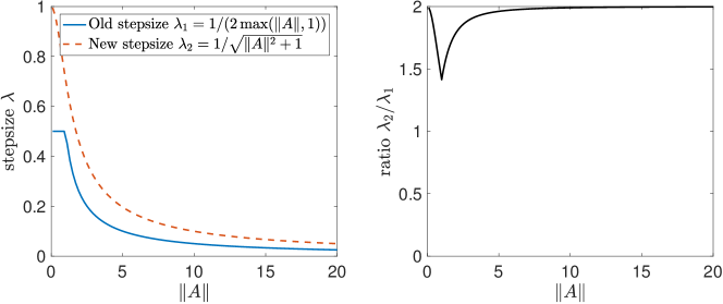
Figure 1: The new analysis allows for a larger stepsize

An advantage of this approach is that we are free to choose $\tau_{x}\neq\tau_{y}\neq\tau_{z}$. For example, choose $\tau_{x}=\|AA^{*}\|$, $\tau_{z}=\|BB^{*}\|=1$, $\tau_{y}<1/2$.

Acknowledgments

The author is grateful to P. Combettes for helpful discussions and introducing the Chen-Teboulle algorithm.

References

• [BC11] H. H. Bauschke and P. L. Combettes, Convex analysis and monotone operator theory in Hilbert spaces, Springer-Verlag, New York, 2011.
• [Con13] L. Condat, A primal-dual splitting method for convex optimization involving Lipschitzian, proximable and linear composite terms, J. Optim. Theory Appl. (2013), 460–479.
• [CP07] P. L. Combettes and J.-C. Pesquet, A Douglas-Rachford splitting approach to nonsmooth convex variational signal recovery, IEEE J. Sel. Topics Signal Processing 1 (2007), no. 4, 564–574.
• [CP10] A. Chambolle and T. Pock, A first-order primal-dual algorithm for convex problems with applications to imaging, J. Math. Imaging Vision 40 (2010), no. 1, 120–145.
• [CT94] G. Chen and M. Teboulle, A proximal-based decomposition method for convex minimization problems, Math. Prog. 64 (1994), no. 1-3, 81–101.
• [EZC10] E. Esser, X. Zhang, and T. Chan, A general framework for a class of first order primal-dual algorithms for convex optimization in imaging science, SIAM J. Imaging Sci. 3 (2010), no. 4, 1015–1046.
• [HY12] B.S. He and X. M. Yuan, Convergence analysis of primal-dual algorithms for a saddle-point problem: from contraction perspective, SIAM J. Imaging Sci. (2012), 119–149.
• [Mor62] J.-J. Moreau, Fonctions convexes duales et points proximaux dans un espace hilbertien, R. Acad. Sci. Paris Sér. A Math. 255 (1962), 2897–2899.
• [Roc70] R. T. Rockafellar, Convex analysis, Princeton Landmarks in Mathematics and Physics, Princeton University Press, Princeton, NJ, 1970.
• [Tse08] P. Tseng, On accelerated proximal gradient methods for convex-concave optimization, SIAM J. Optim., submitted (2008).
• [Vũ13] B. C. Vũ, A splitting algorithm for dual monotone inclusions involving cocoercive operators, Adv. Comput. Math 38 (2013), no. 3, 667–681.
• [ZC08] M. Zhu and T. Chan, An efficient primal-dual hybrid gradient algorithm for total variation image restoration, Tech. Report CAM08-34, UCLA, 2008, Available at ftp://ftp.math.ucla.edu/pub/camreport/cam08-34.pdf.