Adaptive Ensemble of Classifiers with Regularization for Imbalanced Data Classification

Abstract

The dynamic ensemble selection of classifiers is an effective approach for processing label-imbalanced data classifications. However, such a technique is prone to overfitting, owing to the lack of regularization methods and the dependence of the aforementioned technique on local geometry. In this study, focusing on binary imbalanced data classification, a novel dynamic ensemble method, namely adaptive ensemble of classifiers with regularization (AER), is proposed, to overcome the stated limitations. The method solves the overfitting problem through implicit regularization. Specifically, it leverages the properties of stochastic gradient descent to obtain the solution with the minimum norm, thereby achieving regularization; furthermore, it interpolates the ensemble weights by exploiting the global geometry of data to further prevent overfitting. According to our theoretical proofs, the seemingly complicated AER paradigm, in addition to its regularization capabilities, can actually reduce the asymptotic time and memory complexities of several other algorithms. We evaluate the proposed AER method on seven benchmark imbalanced datasets from the UCI machine learning repository and one artificially generated GMM-based dataset with five variations. The results show that the proposed algorithm outperforms the major existing algorithms based on multiple metrics in most cases, and two hypothesis tests (McNemar’s and Wilcoxon tests) verify the statistical significance further. In addition, the proposed method has other preferred properties such as special advantages in dealing with highly imbalanced data, and it pioneers the research on the regularization for dynamic ensemble methods.

Keywords - Adaptive ensemble; Gradient Boosting Machines; Regularization; Imbalanced data classification

1 Introduction

Imbalanced data classification refers to the classification of datasets with significantly different instance numbers across classes [1]. Specifically, for the binary imbalanced data classification problem, there is usually a dominating number of instances from one class (the majority class) and a few instances belonging to the other class (the minority class). The problem of binary imbalanced data classification is common in engineering and scientific practices [2, 3, 4]. The problem is non-trivial, because most of the general-purpose classification methods will overwhelmingly favor the majority class in the label-imbalanced scenario, leading to significant performance degradation. Consequently, the development of binary imbalanced classification algorithms has become an independent and active research area.

Among the popular algorithms for binary imbalanced classification, the dynamic ensemble of classifiers has attracted significant attention. It works by training multiple classifiers using different subsets of the data, and dynamically selecting from, or combining them, during the inference process. By picking the most competent classifier(s) for each specific test instance, this approach can mitigate the “majority favoritism” in imbalanced data classification [5, 6]. There are various advanced algorithms built on the strategy of the dynamic ensemble model, and the novelty of most of them lies in their use of certain new techniques to ‘ensemble’ models. For instance, [7] proposes a generalized mixture function to combine different classifiers, and [8] proposes an adaptive ensemble method based on the classification problem. We review a few similar methods in this paper, and more details are presented in Section 2.

Despite the success of the dynamic ensemble of classifiers with regard to various tasks, we are unaware of any existing model that addresses the overfitting exhibited by such classifiers. Overfitting is a common problem, wherein the behavior of the classifiers overly fit the training data. This adversely affects the performance on the test data, because not all the information in the training data is useful (e.g. noises). At first glance, it appears that the dynamic ensemble of classifiers can safely circumvent the curse of overfitting, because they utilize the test data during the selection of classifiers. However, because each classifier is usually trained using a small subset of data (which contains information from the local geometry only), dynamically picking the most competent of them can lead to the overfitting of the local geometry of these classifiers. Even if we interpolate the dynamic ensemble with a set of (fixed) trained weights for the classifiers, the overfitting problem will persist, as the weights are obtained purely from the training data. Hence, it seems there is no simple solution to the overfitting problem of the dynamic ensemble of classifiers.

We solve the aforementioned problems using the regularization effect arising from gaussian mixture model (GMM)-based resampling and the stochastic gradient descent (SGD) algorithm. The proposed method is called the adaptive ensemble of classifiers with regularization (AER), where the term “with regularization” refers to the two types of regularization schemes that are developed in this study. The AER method first performs data resampling based on the GMM [9, 10]. We will generate two types of subsets. The first type will have a broader inclusion of the points from the majority class, and the second will have an almost balanced number of instances from the two classes. The former type of subsets can force the classifiers to consider the global geometry; therefore, this is the regarded as the first regularization to alleviate the overfitting problem. The latter type of subsets provides information on the local geometries to ensure they fit sufficiently powerful classifiers. After completing the resampling process, one individual classifier is learned for each sampled subset, and we explicitly learn a set of fixed coefficients/weights by optimizing the cross-entropy loss of the combined model with the SGD. The adaptation of the SGD is the second regularization, and its effectiveness has been verified by numerous studies [11, 12, 13, 14]. During the inference procedure, the normalized coefficient of each individual classifier will be determined by a combination of the on-the-fly likelihood and the trained classifier coefficients.

We theoretically and empirically evaluate the performance of the proposed AER. From a theoretical perspective, we analyze the time and space complexity of the AER model, and prove that the seemingly complicated AER model actually requires less time and memory to train. From an empirical perspective, we test the performance of the AER model, using the XGBoost classifier [15] (we refer to the combined method as AER-XGBoost) based on seven imbalanced UCI machine learning datasets and a GMM-generated dataset with five variations. Based on multiple metrics, experimental results reveal that the AER-XGBoost model exhibits competitive performances, outperforming multiple standard methods, such as the SVM and decision tree, and state-of-the-art methods, such as the focal loss neural network [16], vanilla XGBoost [15], focal loss XGBoost [17], and the LightGBM model [18]. The Mcnemar’s and Wilcoxon signed-rank tests are performed to further validate the superior performance of the AER, and the results are mostly sufficient to reject the null hypothesis for performance difference. We note that the AER generally performs significantly better in severe label-imbalanced and complex decision boundary scenarios.

The rest of the paper is structured as follows: Section 3 introduces the algorithm in detail, with its properties. Section 4 analyzes the advantageous time and memory complexity of the proposed algorithm. Experimental Framework and and results analysis are demonstrated in Section LABEL:ExperimentFramework and Section 6 respectively, and related discussions are presented in Section 7. Lastly, Section 8 provides a general conclusion of the paper.

2 Related Work

Imbalanced data classification refers to the classification problem where the number of samples for each class label is not balanced, or, where the class distribution is biased or skewed [1]. Since most of the standard classifiers assume relatively balanced class distributions and equal mis-classification costs, the class-imbalance can be perceived as a form of data irregularity [19], and it could significantly deteriorate the performances of classifiers. Performing high-accuracy classification using imbalanced data has been a challenge for a long time, and there have been considerable number of publications discussing novel methods to address the problem. The methods can be roughly categorized into four branches [20, 21]. The first branch is the re-sampling methods that generate balanced data by under-sampling the majority class, and/or over-sampling the minority instances [22]. The second branch is the cost-sensitive algorithms that address the problem by using imbalance-sensitive target functions, and assigning special loss functions explicitly ([23]) or implicitly ([24, 25, 26]). The third branch is the one-class learning methods that solve the label-imbalance problem by learning the representation of the majority/minority data [27, 28]. The final branch is the ensemble methods that contain the dynamic ensemble of classifiers, as employed in this study.

The idea of the ensemble methods (and, by implication, the dynamic ensemble of classifiers) is to utilize ‘the wisdom of the many’; a typical ensemble method will fit multiple classifiers and/or re-sampled multiple datasets, and then combine them in some way to obtain final predictions [29, 30, 31, 32]. On the other hand, the static ensemble of classifiers approach will complete the training of the individual classifiers and their weights based solely on the training data [33]. This approach requires less computational resource, as the predictions can be obtained using a fixed model. However, when encountering noises in the minority or complex and rapidly changing decision boundary between the classes, the static ensemble methods often suffer performance degradation [34, 33, 35]. On the other hand, the dynamic ensemble methods will change the combination of classifiers on-the-fly, according to the test instances. Compared with its static counterpart, the dynamic ensemble of classifiers introduces greater model flexibility and representation power. Multiple studies have empirically shown that the dynamic ensemble is a more preferred choice, based on different metrics [5, 6, 36].

The dynamic ensemble approach can be roughly divided into two categories: the dynamic classifier selection (DCS) approach, wherein the most competent classifier is selected dynamically ([37]), and the dynamic ensemble selection (DES), wherein multiple classifiers are selected for prediction ([38]). Earlier works in the area often adopt the DCS strategy; for instance, Woods (1997) [37] utilizes a “rank-based” method to select the most competitive classifier. Conversely, because the DES is more flexible, modern scientists have investigated more novel methods based on it. Most of the recent models pin their novelty on the renewed strategies to combine/ensemble the classifiers. For instance, Lin et al. (2014) [39] proposed a method to ensemble classifiers based on clustering results; Cruz et al. (2015) [40] designed an algorithm to combine classifiers using meta-learning; Xiao et al. (2012) [41] introduced cost-sensitive criteria to determine the weights of the ensemble; Krawczyk et al. (2018) [42] used the dynamic ensemble of one-class classifiers to train the model with regard to multiple classes; and Brun et al., (2018) [8] proposed adjusting the ensemble based on the difficulty of classification. Nevertheless, despite the fruitful results in the literature, to the best of our knowledge, we do not know any method under the DES framework wherein regularization is introduced (to avoid overfitting).

We assume that the absence of such research is because there is no obvious approach to introduce regularization to the dynamic ensemble model. Conventional norm-based regularization works by minimizing the norms of the weights; however, in the dynamic ensemble scenario, the weight of each classifier cannot be shrunk, because they should be in the range of $[0,1]$, and sum up to $1$ (a simplex). Other existing regularization techniques are either not applicable to the scenario (e.g., NoiseOut [43], which is designed for neural networks), or considered too “aggressive” for linear combination (e.g., dropout [44], which will block some classifiers entirely). To overcome the above obstacles, the AER is regularized implicitly based on two techniques: global-geometry interpolation and the SGD algorithm. The regularization effect of the first approach is derived from previous ideas on data resampling, and the central idea is to reduce the impact of the noise from the overlap between the classes [45, 46]. The regularization power of the second approach (SGD) is supported by its attribute of converging to a solution with a minimum $\ell_{2}$ norm [47], and multiple theoretical and empirical results have proved its effectiveness [12, 48].

Binary imbalanced classification has a broad range of applications. In bioscience and medical research, imbalanced data classification has been utilized to identify tumor [2], and diagnose cancer [49]. Likewise, in software engineering, it has been employed to detect bugs [50] or malignant software [51]. In other fields, such as financial fraud detection [52] and power transformation [3], imbalanced data classifications are also comprehensively employed. Guo (2017) [1] surveys the applications of imbalanced data classification, and shows the promising potential in applying such a technique to a broader range of problems.

3 Methods

In this section, we introduce the details of the proposed AER model. The structure is laid out as follows: Section 3.1 will introduce the GMM-fitting and generation of the two types of subsets; Section 3.2 will discuss the specific implementation with XGBoost, which is the individual ‘base’ classifiers used in the experiments; the SGD training for the ensemble of classifiers will be illustrated in Section 3.3; and finally, the weight interpolation/combination and probabilistic prediction will be shown in Section 3.4. The overall procedure of the algorithm is shown in Figure 1.

Before diving into the details, we shall specify the notations that will be used. We use $\boldsymbol{x}$ to denote a single instance of the data in the dataset $\boldsymbol{X}$. To distinguish the majority and minority data, we use $\boldsymbol{X}_{k}$ (key data, usually the minority) to denote the set of minority data and $\boldsymbol{X}_{n}$ (non-key data, usually the majority) to represent the set of majority data. The size of the dataset is denoted by $m$, and the dimension (the number of features) is represented by $n$; we use $m_{k}$ and $m_{n}$ to denote the number of points of the minority and the majority data. Finally, $L$ denotes the number of Gaussian distributions in the GMM, and $2L$ is the number of classifiers, according to our setup.

Figure 1: The overall process of the proposed AER algorithm

3.1 Gaussian Mixture Model Fitting and Subset Generation

The GMM is a popular model in unsupervised learning and data manifold representation. The basic idea behind the GMM is straightforward; it utilizes the modeling capability of the Gaussian distribution, and extends it to multiple centroids to improve the expressiveness. The likelihood of a single instance in the GMM can be denoted as follows:

$$p(\boldsymbol{x}|\{\boldsymbol{\mu}_{l},\boldsymbol{\Sigma}_{l},w_{l}\})=\sum_{l=1}^{L}w_{l}\mathcal{N}(\boldsymbol{x}|\boldsymbol{\mu}_{l},\boldsymbol{\Sigma}_{l})$$ (1)

where $\mathcal{N}(\cdot|\boldsymbol{\mu},\boldsymbol{\Sigma})$ denotes a multivariate Gaussian distribution, with $\boldsymbol{\mu}$ as the mean and $\boldsymbol{\Sigma}$ as the co-variance. When fitting the model, the parameters can be obtained by maximizing the log-likelihood:

$$\{\hat{\boldsymbol{\mu}}_{l},\hat{\boldsymbol{\Sigma}}_{l},\hat{w}_{l}\} =\operatorname*{arg\,max}_{\boldsymbol{\mu}_{l},\boldsymbol{\Sigma}_{l},w_{l}}\log(\prod_{i=1}^{m}\sum_{l=1}^{L}w_{l}\mathcal{N}(\boldsymbol{x}_{i}|\boldsymbol{\mu}_{l},\boldsymbol{\Sigma}_{l}))$$ (2)

$$=\operatorname*{arg\,max}_{\boldsymbol{\mu}_{l},\boldsymbol{\Sigma}_{l},w_{l}}\sum_{i=1}^{m}\log(\sum_{l=1}^{L}w_{l}\mathcal{N}(\boldsymbol{x}_{i}|\boldsymbol{\mu}_{l},\boldsymbol{\Sigma}_{l}))$$

Equation 2 can be solved using an expectation-maximization (E-M) algorithm with a super-linear convergence rate [53]. In our program, the package of the GMM provided by SciKit-learn [54] is directly adopted, to perform the fitting procedure of the GMM.

It may be observed that the GMM is sensitive to initialization. To obtain stable results, the optimization will be performed $5$ times for each training procedure, and the model with the highest log-likelihood will be selected. Another non-learnable parameter in the GMM is the number of Gaussian distributions. In the proposed algorithm, this hyper-parameter also determines the number of components in the final ensemble. To obtain the optimal number of components that optimally balances the likelihood and computational complexity, the Bayesian information criterion (BIC) is adopted. The BIC metric can be computed as follows:

$$\text{BIC}=\log(m)\|\boldsymbol{f}\|-2\sum_{i=1}^{m}\log p(\boldsymbol{x}_{i})$$ (3)

where $\|\boldsymbol{f}\|$ stands for the number of the parameters of the model, and $p(\boldsymbol{x}_{i})$ indicates the likelihood of the instance $\boldsymbol{x}_{i}$. In terms of the GMM presented in our method, the BIC will be computed as follows:

$$\text{BIC}=\log(m)\|\boldsymbol{f}\|-2\sum_{i=1}^{m}\log(\sum_{l=1}^{L}w_{l}\mathcal{N}(\boldsymbol{x}_{i}|\boldsymbol{\mu}_{l},\boldsymbol{\Sigma}_{l}))$$ (4)

In the training process, a “pool” of the possible numbers of Gaussian centroids will be given, and the algorithm will compute the BIC of each model, and pick the one with the least BIC. We choose the BIC over the Akaike information criterion (AIC), because the BIC tends to favor the model that overfits the data less [55]. Because regularization plays an important role in our algorithm, the BIC is adopted as the choice of hyper-parameter.

After obtaining the GMM with $L$ Gaussian distributions, we form $2L$ sub-datasets based on two types of schemes. The first type of scheme will be selecting $\lfloor\frac{m_{n}}{L}\rfloor$ most representative data from each of the Gaussian distribution. Specifically, for each Gaussian distribution $\mathcal{N}(\boldsymbol{x}_{i}|\boldsymbol{\mu}_{l},\boldsymbol{\Sigma}_{l})$, the algorithm will select $\lfloor\frac{m_{n}}{L}\rfloor$ instances with the highest log-likelihood. For the second type of paradigm, the algorithm will generate $L$ subsets with $m_{l}$ majority instances selected based on the highest likelihoods, with respect to each Gaussian component, and concatenate it with the $\lfloor 0.5*m_{l}\rfloor$ majority instances randomly selected from the set. Both of the generated majority datasets will be combined with all the minority instances.

After obtaining the above data, a Tomek link [56] will be used to remove instances considered as noises from the first type of data subsets. Tomek links are based on the idea that if two instances are mutually nearest neighbors that belong to different classes, they would be ’overlapping’ instances between classes, and be likely to be noises. Formally, for two given data instances $\{\boldsymbol{x}_{i},\boldsymbol{x}_{j}\}\in\boldsymbol{X}$ and given distance measure $d(\cdot,\cdot)$, if for any $\boldsymbol{x}_{k}\in\boldsymbol{X}$, the following exists:

$$\begin{cases}d(\boldsymbol{x}_{i},\boldsymbol{x}_{j})<d(\boldsymbol{x}_{i},\boldsymbol{x}_{k})\\ d(\boldsymbol{x}_{i},\boldsymbol{x}_{j})<d(\boldsymbol{x}_{j},\boldsymbol{x}_{k})\end{cases}$$ (5)

Then, $\{\boldsymbol{x}_{i},\boldsymbol{x}_{j}\}$ will be considered a pair of Tomek link. If the corresponding labels $\{y_{i},y_{j}\}$ of the Tomek link pair belong to different classes, then we regard the majority and/or minority instance in the pair as noise, and remove one or both of them. In our algorithm, because the minority will be the more important part to be spotted, the majority instances in the Tomek links will be removed.

By performing the above process, there will be $2L$ available sub-datasets, with less significant skewness of labels. As we have explained above, the reason for adopting a combination of two type of re-sampling methods is that this strategy can separately achieve two different goals satisfactorily. The first type of subset can preserve the information of the global geometry, and contribute to the recognition of the majority instances; this helps the AER to avoid overfitting on the overlapping parts between the majority and the minority instances (i.e., a ‘zoom-out perspective’ to ‘pull back’ the decision boundary from the complexity overlapping part between the two classes). The second type of subset emphasizes the local geometry, and improves the accuracy of spotting minority instances (i.e. a “zoomed-in perspective” to focus on learning the complex decision boundary on the overlapping part). Furthermore, because the second type of datasets focus only on the local geometry, we will concatenate them with $\lfloor 0.5*m_{k}\rfloor$ majority instances randomly selected to prevent the decision boundary that is away from the local part from “going wild.”

The overall procedure of the GMM-fitting and subset generation is depicted as Algorithm 1.

Data: majority data $\boldsymbol{X}_{n}$, minority data $\boldsymbol{X}_{k}$, candidate numbers for $L$

Result: Gaussian Mixture Model $\{w_{l},\boldsymbol{\mu}_{l},\boldsymbol{\Sigma}_{l}\}_{l=1:L}$, $2L$ balanced datasets

for $L_{i}$ in candidate $L$ values do

       for $trial\leftarrow 1$ to $5$ do

             initialize Gaussian Mixture Model parameters;

             optimize Gaussian Mixture Model with equation 2 via E-M algorithm;

            

       end for

      Retrieve the model with the highest log-likelihood;

       Compute corresponding BIC using equation 4;

      

end for

Select the model with the smallest BIC value;

for $i\leftarrow 1$ to $L$ do

       select $\lfloor\frac{m_{n}}{L}\rfloor$ most relevant samples from $\boldsymbol{X}_{n}$, according to the log-likelihood of the Gaussian centroid $i$;

       combine the obtained data with $\boldsymbol{X}_{k}$ to form the first type of subset $\boldsymbol{\hat{X}}_{k}$;

       select $m_{k}$ most relevant samples from $\boldsymbol{X}_{n}$, according to the log-likelihood of Gaussian centroid $i$ and combine them with $\lfloor 0.5*m_{k}\rfloor$ randomly selected majority instances;

       combine the obtained data with $\boldsymbol{X}_{k}$ to form the second type of subset $\boldsymbol{\check{X}}_{k}$;

       perform a Tomek link removal for $\boldsymbol{\hat{X}}_{k}$ with equation provided as the condition 5;

      

end for

Algorithm 1 Gaussian Mixture Model Fitting and Balanced Data Generating

3.2 Fitting of Individual Base Classifier

As has been stated above, the specific classifier implemented in this study is the gradient boosting machine (GBM) ([57]), a boosting-based algorithm. The GBM model can be expressed as follows:

$$G_{T}(\boldsymbol{X};\{\boldsymbol{\theta}_{t}\}_{t=1,2,..,T})=\sum_{t=1}^{T}\alpha_{t}g_{t}(\boldsymbol{x};\boldsymbol{\theta}_{t})$$ (6)

Similar to other boosting methods, the training strategy of the GBM is to learn from previous mistakes. Specifically, the individual sub-model of the GBM at the $T$-th step will set the gradient of the loss function, with respect to the model, up to $(T-1)$-th step as the current ‘labels’, which can be expressed as follows:

$$r_{T-1}=-\frac{\partial L(\boldsymbol{y},G_{T-1}(\boldsymbol{X};\{\boldsymbol{\theta}_{t}\}_{t=1,2,..,T-1}))}{\partial G_{T-1}(\boldsymbol{X};\{\boldsymbol{\theta}_{t}\}_{t=1,2,..,T-1})}$$ (7)

where $L(\cdot,\cdot)$ is used to denote any kind of loss function, and is usually the square loss for regression and the cross-entropy loss for classification. The gradient computed with equation 7 is also named the ‘pseudo-residual’; because the gradient will be calculated at each step, the overall method is tagged the GBM. After obtaining the current target, the parameter of the sub-model at the $T$-th step can be denoted as follows:

$$\boldsymbol{\theta}_{T}=\operatorname*{arg\,min}_{\boldsymbol{\theta}}L(r_{T-1},G(\boldsymbol{X};\boldsymbol{\theta}))$$ (8)

The overall model at the $T$-th step is further determined by a ’learning rate’ $\alpha_{T}$ that can be obtained by optimizing the following target function:

$$\alpha_{T}=\operatorname*{arg\,min}_{\alpha}L(\boldsymbol{y},G_{T-1}(\boldsymbol{X};\{\boldsymbol{\theta}_{t}\}_{t=1,2,..,T-1})+\alpha g(\boldsymbol{X};\boldsymbol{\theta}_{T}))$$ (9)

The above optimization can be simply solved, either by taking partial derivative or through a line search. By iterating the procedure from Equation 7 to 9, until it matches the convergence criteria, the integrated GBM model will be obtained.

In our implementation, an integrated, high-efficient, and scalable gradient boosting interface, XGBoost [15], is employed to fit, and make prediction with the GBM. For each sub-set of data generated, the algorithm will fit one XGBoost model, denoting as $f_{l}(\cdot)$.

3.3 Stochastic Gradient Descent Training for the Ensemble of Classifiers

After the training with the individual models, each classifier will be able to give a class prediction (0 or 1) for every data instance. The next step is to train the combination of individual classifiers using the SGD algorithm. For convenience, each individual model will be denoted as $f_{l}(\cdot)$. We can denote the linear combination of the models as follows:

$$F(\boldsymbol{X}) =\sum_{l=1}^{2L}w_{l}*f_{l}(\boldsymbol{X})$$ (10)

$$\text{s.t. }\begin{aligned} &\sum_{l=1}^{2L}w_{l}=1\\ &0\leq w_{l}\leq 1,\quad\forall l\in\{1,2,...,2L\}\end{aligned}$$

The constraints of Equation 10 is to guarantee that the values of the predictions will be between $[0,1]$; thus, it could simply be transferred to a binary-class prediction. To train the model, the two-class cross-entropy loss is adopted:

$$L(\boldsymbol{y},\boldsymbol{X}) =-\sum_{i=1}^{m}y_{i}\log(\sum_{l=1}^{2L}w_{l}\cdot f_{l}(\boldsymbol{x}_{i}))+(1-y_{i})\log(1-\sum_{l=1}^{2L}w_{l}\cdot f_{l}(\boldsymbol{x}_{i}))$$ (11)

$$=-\sum_{i=1}^{m}y_{i}\log(\boldsymbol{w}^{T}\boldsymbol{f}(\boldsymbol{x}_{i}))+(1-y_{i})\log(1-\boldsymbol{w}^{T}\boldsymbol{f}(\boldsymbol{x}_{i}))$$

where the second line of the above equation is the vectorized expression. Note that because there is a constraint on $\boldsymbol{w}$, the above optimization cannot be accomplished by simply taking derivatives and setting them to 0. Furthermore, to perform the SGD algorithm, the gradient of the target 11, with respect to $\boldsymbol{w}$ should be as follows:

$$\frac{\partial L(\boldsymbol{y},\boldsymbol{X})}{\partial\boldsymbol{w}} =-\sum_{i=1}^{m}(\frac{y_{i}}{\boldsymbol{w}^{T}\boldsymbol{f}(\boldsymbol{x}_{i})}-\frac{1-y_{i}}{(1-\boldsymbol{w}^{T}\boldsymbol{f}(\boldsymbol{x}_{i}))})\boldsymbol{f}(\boldsymbol{x}_{i})$$ (12)

$$=\sum_{i=1}^{m}(\frac{1}{(1-y_{i})-\boldsymbol{w}^{T}\boldsymbol{f}(\boldsymbol{x}_{i})})\boldsymbol{f}(\boldsymbol{x}_{i})$$

If gradient descent is applied, the gradient in equation 12 does not guarantee that the sum of $\boldsymbol{w}$ will be 1, neither does it warrant that each $w_{k}$ will be in the interval of $[0,1]$. We provide a simple remedy to this; we can simply re-normalize the weight after learning. In addition, for the weights exceeding the limit of the interval, we can re-scale them to the limit value (0 or 1). In this way, the update formula of $\boldsymbol{w}$ should be as follows:

$$\boldsymbol{w}_{t+1} =\frac{S(\boldsymbol{w}_{t}-\gamma_{t}\nabla_{\boldsymbol{w}_{t}}L(\boldsymbol{y},\boldsymbol{X}))}{\sum_{l=1}^{L}S(\boldsymbol{w}_{t}-\gamma_{t}\nabla_{\boldsymbol{w}_{t}}L(\boldsymbol{y},\boldsymbol{X}))_{l}}$$ (13)

$$=\frac{S(\boldsymbol{w}_{t}-\gamma_{t}\sum_{i}^{m}(\frac{1}{(1-y_{i})-\boldsymbol{w}_{t}^{T}\boldsymbol{f}(\boldsymbol{x}_{i})})\boldsymbol{f}(\boldsymbol{x}_{i}))}{\sum_{l=1}^{L}S(\boldsymbol{w}_{t}-\gamma_{t}\sum_{i}^{m}(\frac{1}{(1-y_{i})-\boldsymbol{w}_{t}^{T}\boldsymbol{f}(\boldsymbol{x}_{i})})\boldsymbol{f}(\boldsymbol{x}_{i}))_{l}}$$

where $\gamma_{t}$ is the learning rate, and $S(\cdot)$ denotes the re-scaling(mapping) function floor at 0 and ceiling at 1. This can be mathematically denoted as follows:

$$S(x)=\frac{x-x_{min}}{x_{max}-x_{min}}$$ (14)

It is recommended that the learning rate should be set less than $\frac{1}{||\nabla_{\boldsymbol{w}_{t}}L(\boldsymbol{y},\boldsymbol{X})||}$, to ensure convergence. To determine whether the training procedure has converged, the relative change in the cross-entropy loss is adopted as the metric.

Another concern regarding using the SGD method is how to initialize the coefficients, as the optimization is sensitive to initial values. In the proposed algorithm, the initialization of parameters is accomplished by the combination of the AIC and BIC. Similar to the BIC, the AIC can be expressed as follows:

$$\text{AIC}=2\|\boldsymbol{f}\|-2\sum_{i=1}^{m}\log(p(\boldsymbol{x}_{i}))$$ (15)

where $p(\boldsymbol{x}_{i})$ indicates the likelihood of instance $\boldsymbol{x}_{i}$. Combining equations 3 and 15, we could compute a combined metric as follows:

$$\boldsymbol{\tilde{w}}_{l}=\lambda_{A}\cdot\text{AIC}_{l}+(1-\lambda_{A})\cdot\text{BIC}_{l}$$ (16)

where $\lambda_{A}$ is the parameter for striking a balance between the AIC and BIC; experiments demonstrate that $\lambda_{A}=0.6$ could be an effective trade-off. Here, the AIC and BIC are computed with respect to each classifier, and lower AIC/BIC values indicate a more credible solution. Thus, we can use the normalized reciprocal of $\boldsymbol{\tilde{w}}_{l}$ values to initialize the linear combination. The initial values can be denoted as follows:

$$\boldsymbol{\hat{w}}_{k}=\frac{1/\boldsymbol{\tilde{w}}_{l}}{\sum_{l=1}^{2L}(1/\boldsymbol{\tilde{w}}_{l})}$$ (17)

The overall procedure of the optimization of the linearly combined base classifiers can be denoted as Algorithm 2.

Data: Individual Classifiers $\boldsymbol{f}_{l}(\cdot)$, Corresponding Balanced Data set $\boldsymbol{X}$(including $\boldsymbol{\hat{X}}$ and $\boldsymbol{\check{X}}$), where $l=1,2,...,2L$

Result: Trained Combination of Models $F(\cdot)$

Initialize the linear combination model with equation 17;

for $t\leftarrow 1$ to Max-Step do

       Compute the current gradient with equation 12;

       Update the weights with equation 13;

       Compute the current cross-entropy loss with equation 11;

       if Cross-Entropy Loss Change $\leq$ tol then

             break;

            

       end if

      

end for

Algorithm 2 Stochastic Gradient Descent Training of Linear Ensemble of Base Classifiers

3.4 Weight Computation and the Probabilistic Prediction

The preceding three sections have discussed generating balanced sub-datasets, and training individual and combined classifiers. As a dynamic ensemble method, the coefficient of each individual classifier should be on-the-fly, according to the test instance(s). Because we have multiple ‘base’ classifiers, and each of them is trained by its corresponding subset, it makes sense to pick the most effective ones, based on the test data. Our selection strategy is to compute the ’distance’ (denoted by the likelihood) between the specific test instance and the Gaussian centroids. Intuitively, a higher likelihood indicates a more significant impact on the test instance, and we can assign more ‘credit’ to the corresponding classifiers. Based on the above idea, we propose computing the on-the-fly weights with two types of likelihoods, based on the logarithm and exponential (original) forms, respectively. More concretely, for any test instance $\boldsymbol{x}^{*}$, the component of the normalized likelihood $\boldsymbol{l}^{*}$ will be as follows:

$$\boldsymbol{l}^{*}=\begin{cases}\frac{\log\mathcal{N}(\boldsymbol{x}^{*}|\boldsymbol{\mu}_{l},\boldsymbol{\Sigma}_{l})}{\sum_{l=1}^{2L}\log\mathcal{N}(\boldsymbol{x}^{*}|\boldsymbol{\mu}_{l},\boldsymbol{\Sigma}_{l})},&\text{ Log-likelihood}\\ \frac{\mathcal{N}(\boldsymbol{x}^{*}|\boldsymbol{\mu}_{l},\boldsymbol{\Sigma}_{l})}{\sum_{l=1}^{2L}\mathcal{N}(\boldsymbol{x}^{*}|\boldsymbol{\mu}_{l},\boldsymbol{\Sigma}_{l})},&\text{ Exp-likelihood}\end{cases}$$ (18)

In the above equation, because the global geometry is considered (especially in the normalization), the on-the-fly weights are regularized. Finally, for the purpose of the SGD-induced regularization, we will interpolate the on-the-fly weights with the learned static ones:

$$\boldsymbol{w}^{*}=\lambda\boldsymbol{l}^{*}+(1-\lambda)\boldsymbol{w}$$ (19)

where the “$+$” operation stands for pairwise summation. $\lambda$ is the interpolation parameter, and the optima can be found via the training or the validation data through grid search. It is easy to verify that the results computed by equation 19 satisfy the condition that the sum should be equal to 1, and the value of each coefficient will be in the interval $[0,1]$.

Following the above procedure, the algorithm will compute a probabilistic value $\boldsymbol{w}^{T}f(\boldsymbol{x}^{*})\in[0,1]$ for each test point $\boldsymbol{x}^{*}$. The output can be regarded as the probability of $p(\boldsymbol{y}^{*}=1|\boldsymbol{x}^{*})$, and instead of simply setting all samples greater than $0.5$ as $1$, and less, as $0$, the threshold can be tuned, based on the following equation:

$$F(\boldsymbol{x}^{*})=\begin{cases}1,\boldsymbol{w}^{T}f(\boldsymbol{x}^{*})\geq\delta\\ 0,\boldsymbol{w}^{T}f(\boldsymbol{x}^{*})<\delta\end{cases}$$ (20)

where $\delta$ can be regarded as a ”threshold value,” and the optima can be found via the validation data through grid search.

The overall procedure of the proposed AER with the XGBoost implementation (AER-XGBoost) can be depicted as algorithm 3.

Data: Imbalanced Data Set with Data Separated as $\boldsymbol{X}_{n}$ and $\boldsymbol{X}_{k}$; Test Data Set $\boldsymbol{X}^{*}$

Result: Label Predictions using the overall model $F(\boldsymbol{X}^{*})$

Performe the GMM-fitting for the majority class, and generate $2L$ balanced subsets, based on the algorithm 1;

for $l\leftarrow 1$ to $2L$ do

       Initialize the current XGBoost Model $\boldsymbol{f}_{l}(\cdot)$;

       for $t\leftarrow 1$ to Maximum-Boosting-Depth do

             Update the XGBoost Model according to equations 7-9;

            

       end for

      Store the current model $\boldsymbol{f}_{l}(\cdot)$;

      

end for

Linearly combining the models with coefficients learned from Algorithm 2;

Use the validation or the training data to find the optimal $\lambda$ value and $\delta$ value

for each test point $\boldsymbol{x}^{*}$ do

       Compute the interpolated weight $\boldsymbol{l}^{*}$ of instance $\boldsymbol{x}^{*}$ with equation 18;

       Update the weights $\boldsymbol{w}^{*}$ through equation 19;

       Predict the current label $F(\boldsymbol{x}^{*})$ with equation 20;

      

end for

Algorithm 3 Overall Algorithm

4 Theoretical Analysis of the AER

In this section, we will demonstrate that the proposed AER method has advantageous time and memory complexity. Specifically, we will show theoretically that, under certain assumptions and for any classifier implemented with the AER framework, the time complexity will be, asymptotically, at least as good as the original implementation, and the asymptotic memory complexity will always be better than the full-batch implementations.

To begin with, let us recap the notations used in the AER model. Recall that $m$ denotes the number of instances, and $n$ represents the number of features. $m_{k}$ and $m_{n}$ are used for the minority and majority data, respectively. The skew rate here will be denoted as $R$; it is straightforward to deduce that $m_{n}=R\cdot m_{k}$. The number of Gaussian centroids is given as $L$, and, in most cases, $L<R$, as it will otherwise miss the purpose of re-sampling (it is possible to simply train balanced sub-sets, and include all the training set). This also implies that $L<m$ as $m=(R+1)m_{k}\geq(R+1)>L$. The number of iterations of the GMM E-M algorithm will be denoted as $t_{1}$, and the number of iterations of the SGD algorithm is denoted by $t_{2}$. The time complexity of any machine learning classifier $T(m,n)$ can be denoted as a polynomial of the numbers of instances and features $T(m,n)=O(m^{a}n^{b})$, where $a$ and $b$ should be positive integers. Similarly, we will denote the memory complexity using $M(m,n)=O(m^{a}n^{b})$. We are preoccupied mostly with the complexity of the training process, as this will usually be the part that consumes most of the time and memory.

To derive a boundary that is not dependent on the GMM-fitting or SGD part, and draw fair comparisons between the AER-implemented methods and the original methods, the analysis will be based on the assumption that the GMM covariance inversion and likelihood will be estimated through the diagonal covariance approximation. This will remove high-order terms of $n$, and reduce the time complexity of computing the GMM to $O(mn)$, as the inversion and multiplication of the covariance can be completed within $O(n)$ time. Further, we assume the choice of $\lambda$ and $\delta$ is based on the validation set, and its size is considerably smaller, with the condition $m=\Omega(m_{v}L)$, where $m_{v}$ is the number of validation data points.

4.1 Time Complexity

For any machine learning method with polynomial training time complexity $T(m,n)=O(m^{a}n^{b})$, the AER time complexity can be denoted as $T^{AER}(m,n)$. Under the assumptions stated above, the following theorem can be derived:

Theorem 1.

Assuming $t_{1}=O(\log(m))$ and $t_{2}\leq n\cdot R/L$, the following property holds: If $a=1$, which means $T(m,n)\in\tilde{O}(mn^{b})$, then, there will be $T^{AER}(m,n)\in\tilde{\Theta}(T(m,n))$; otherwise, if $a\geq 2$, which means $T(m,n)\in\Omega(m^{2}n^{b})$, then, there will be $T^{AER}(m,n)\in o(T(m,n))$. Both $\tilde{O}(\cdot)$ and $\tilde{\Theta}(\cdot)$ hide polylog terms.

Proof.

The theorem can be proved by a simple analysis. The memory complexity of the AER method can be decomposed into four parts: the complexity of computing the GMM model, the training complexity of the individual classifiers, the SGD, and the validation part to obtain the optimal $\delta$ and $\lambda$. Each part will have the following complexity:

• Fitting the GMM model. The algorithm will fit the $2L$ Gaussian distributions; it will take $L\cdot O(t_{1}\frac{m}{L}n)+L\cdot O(t_{1}\frac{m}{R}n)$ to fit the models under diagonal covariance. The overall complexity will be $O(t_{1}mn)$. Observe that $L<R$ is used in the derivation.

• Training individual classifiers. For the first type of re-sampled data, the number of training instances will be $\hat{m}=O(\frac{m_{n}}{L}+m_{k})=O(\frac{R}{L}m_{k})=O(\frac{m}{L})$; for the second type of re-sampled data, the amount of training samples will be $\hat{m}=2.5m_{k}=O(m_{k})=O(\frac{m}{R})$. Given the polynomial-form time complexity $T(m,n)=O(m^{a}n^{b})$, the complexity of this part will be $L\cdot[O({(\frac{m}{L})}^{a}n^{b})+O({(\frac{m}{R})}^{a}n^{b})]=O(L{(\frac{m}{L})}^{a}n^{b})=O({\frac{m^{a}}{L^{a-1}}}n^{b})$.

• Stochastic gradient descent. This part will take $O((m_{n}+b_{N})Lt_{2})$, where $b_{N}$ is the batch size of the SGD, and $t_{2}$ is the number of iterations. $b_{N}$ is a constant, and can therefore be hidden asymptotically, resulting in $O(m_{n}Lt_{2})=O(\frac{mLt_{2}}{R})$ runtime.

• Validation of the optimal $\lambda$ and $\delta$ parameters. Under the option of diagonal covariance approximation, the likelihood estimation of a single data point will be $O(Ln)$. It is estimated that all the sets are $O(Lm_{v}n)$. The optimal $\lambda$ and $\delta$ values need to be obtained via multiple running times; however, the factor can be hidden, as it will be a constant.

Summarizing the above terms, the overall complexity will be $O(t_{1}mn+{\frac{m^{a}}{L^{a-1}}}n^{b}+\frac{mLt_{2}}{R}+Lm_{v}n)$. Because the condition is given as $t_{2}\leq\frac{nR}{L}$ and $m,n\geq 1$, the third term can be hidden. Furthermore, because we assumed a large training set and a small validation set with $m=\Omega(m_{v}L)$, the final part can be hidden, and the complexity will be $T^{AER}(m,n)=O({\frac{m^{a}}{L^{a-1}}}n^{b})$.
Now for the two cases:

• If $a=1$, it could deduced that $T^{AER}(m,n)=O(t_{1}mn+{\frac{m}{L^{0}}}n^{b})=O(m\log(m)\cdot n+mn^{b})=\tilde{\Theta}(T(m,n))$.

• If $a\geq 2$, there will be $T^{AER}(m,n)=O(m\log(m)\cdot n+{\frac{m^{a}}{L^{a-1}}}n^{b})=o(m^{a}n^{b})=o(T(m,n))$.

∎

Because the E-M algorithm used to compute the GMM model converges super-linearly, the assumption of $t_{1}=O(\log(m))$ is not far from the reality. Theorem 1 indicates that by re-sampling the dataset, the proposed AER method can reduce the time complexity, when the original complexity is super-linear, with respect to the amount of data $m$, and will not be worse than the original full-batch implementation, when the complexity is linear to $m$.

Table 1 presents the comparison results of the time complexity among common machine learning classifiers implemented using the original full-batch scheme and the AER framework. From the table, it can be observed that the higher the order of $m$ in an algorithm, the more advantages the AER framework will bring. The GBM, which is the method-of-choice in our base classifier, is also listed in the table, and $|T|$ denotes the number of trees in the algorithm. It can be observed that our implementation of the GBM is based on the XGBoost, a parallelized GBM method; furthermore, our implementation does not conform to the polynomial-time regime of our analysis. Nevertheless, the rigorous analysis of the time complexity provides a convincing proof of the advantage of the proposed AER method.

Table 1: Comparison of training time complexity between common Machine Learning classifiers implemented via full-batch original scheme and AER

	original scheme	AER
Naive Bayes	$mn$	$mn$
Decision Tree	$m^{2}n$	$\frac{m^{2}}{L}n$
Non-linear SVM	$m^{3}n$ or $m^{2}n$	$\frac{m^{3}}{L^{2}}n$ or $\frac{m^{2}}{L}n$
Gradient Boosting	$mn|T|$	$mn|T|$

4.2 Memory Complexity

For any machine learning method with polynomial-training memory complexity $M(m,n)=O(m^{a}n^{b})$, the AER memory complexity can be denoted as $M^{AER}(m,n)$. Based on the assumptions stated above, the following theorem can be obtained:

Theorem 2.

For any $a,b\in N^{+}$, $M^{AER}(m,n)\in o(M(m,n))$

Proof.

Similar to the analysis of the time complexity, the memory complexity of the AER is decomposed into four parts:

• Fitting the GMM model. The model needs to store $n$ values under the setting of diagonal variance; thus, the memory complexity will be $O(nL)$.

• Training the individual classifiers. Similar to the time complexity proof, the two types of subsets will have the number of samples in $O(\frac{m}{L})$ and $O(\frac{m}{R})$, respectively. One difference here is that for the memory complexity, one could use the same memory for every Gaussian component. Thus, the memory complexity will be $O((\frac{m}{L})^{a}n^{b})$.

• Stochastic gradient descent. One only needs to keep $2L$ slots in the memory, to update the weights such that the memory complexity will be $O(L)$.

• Validation of the optimal $\lambda$ and $\delta$ parameter. For each Gaussian component, the validation process will take $O(n)$ memory, and each data point will need $O(nk)$. The likelihood of the $m$ data will be stored, which means there should be an additional $O(m)$ complexity. The overall complexity of this part will be $O(m+nk)$.

The final complexity will be given as $O(nL+(\frac{m}{L})^{a}n^{b}+L+nL)=O(nL+(\frac{m}{L})^{a}n^{b})$. Further, because $L<m$, the complexity can be simplified as $O((\frac{m}{L})^{a}n^{b})$, with a simple derivation, one could obtain $M^{AER}(m,n)=O((\frac{m}{L})^{a}n^{b})=O(\frac{m^{a}}{L^{a}}n^{b})=o(m^{a}n^{b})=o(M(m,n))$ ∎

It can be observed that the theory of memory complexity is a stronger conclusion than that of time. Firstly, it removes the restrictions on the iteration times, and the memory complexity is unconditionally bounded. Secondly, the theorem 2 proves a strict upper bound with the little-oh notation (which indicate strictly slower growth asymptotically), regardless of the choice of $a$.

5 Experimental Analysis: the Framework

In this section, we introduce the framework of our empirical analysis for the AER model. We introduce the datasets in section 5.1 with their backgrounds and characteristics. The methods compared against the AER model are discussed in section 5.2, and the metrics to evaluate the results are presented in section 5.3. Finally, we discuss our approaches for statistical testing to validate the significance of the results in section 5.4.

5.1 Datasets

We introduce 12 imbalanced datasets to evaluate the performance of the proposed AER method. Seven of them are from the UCI machine learning repository(Bioassay, Abalone (originally from [58]), Ecoli, US Crime, Wine Quality, Scene and Car Eval), and are regarded as benchmark datasets for imbalanced binary classification. For the Bioassay dataset, we adopt the AID 362 collection, and split it with the train/test ratio of $4:1$. Table 2 shows the statistics of these datasets. In addition, we provide five artificially generated imbalanced datasets sampled from 8,9,10,11,12-center Gaussian Mixture Models, respectively. Because of space limitation, we select the Bioassay, Abalone and the $9$-center GMM-based dataset to demonstrate the detailed information, including the evaluation metrics, the hypothetical testing results, and the curves of the changes on accuracy with different threshold parameter $\delta$. For the Bioassay dataset, we further plot the SGD-trained weights and the change in accuracy, with respect to the interpolation parameter $\lambda$, to offer more insights into the model. For the remaining five UCI datasets and other variations of the GMM-generated data, we only report the results of the evaluation metrics and the results of the statistical tests.

Table 2: Statistics of seven Datasets from UCI Machine Learning Repository

Dataset Name	Number of Samples	Imbalance Ratio	Number of Features
Bioassay	4279	1:70	118
Abalone	4174	1:129	8
Ecoli	336	1:8.6	7
US Crime	1994	1:12	100
Wine Quality	4898	1:26	11
Scene	2407	1:13	294
Car Eval	1728	1:12	21

Table 2 shows the meta-information about the UCI datasets we used in this section. We observe that among the datasets, Bioassay and Abalone have the most significant imbalance ratio. Thus, presenting more details through experiments with these two datasets can help us understand the merits of the AER more clearly. Among all the other datasets, Ecoli is significant for its small size, which can lead to problems for some data-hungry machine learning methods (e.g. focal loss neural Networks). The Scene dataset is of a higher dimension (a greater number of features), and in the corresponding section, we will demonstrate that the AER can perform particularly well, when such rich-information data is provided.

The GMM-based data are introduced to verify that the AER model follows the intuition, because the data geometry is truly from a GMM distribution. A set of 8000 samples is generated through the sk-learn Make-Classification() method, and the imbalance ratio is 1:79, which indicates that 7900 samples are labeled as “0,” and 100, as “1.” Notice that the “number of Gaussian centers” is applied to both the majority and minority data, which means the 100 positive-labeled samples are also from the GMM with 8-12 clusters (depending on the variation). This poses a significant challenge; the algorithms have to learn a complex decision boundary, while preserving a qualified generalization ability. As shall be seen in the corresponding section, the proposed method performs well on this dataset, whereas some other methods, including some state-of-the-art models, completely lose their ability to grasp anything meaningful.

5.2 Compared Methods

We compare seven methods with the proposed AER model with the XGBoost implementation (AER-XGBoost). Among the seven, three are benchmark binary classification methods, which are the (cost-sensitive) SVM, (cost-sensitive) decision tree and a (3-layer) focal loss neural network. The neural network model is engineered with the recently proposed focal loss ([16]) to tackle the label-imbalance problem. To introduce some more novel and advanced methods for comparison, we adopted three more recent methods, the XGBoost ([15]), LightGBM ([18]), and Focal-XGBoost ([17]). Among these three methods, the XGBoost is also adopted as the sub-classifier of the AER model; we can therefore straightforwardly evaluate the benefits brought by the AER framework (in comparison with the vanilla version and other imbalance-augmentation methods, e.g., focal loss). Finally, we also report the results based on the pure dynamic ensemble, which can help validate the contribution of the regularization introduced by the AER.

It is noticeable that apart from the UCI Bioassay data, all the other datasets are not partitioned into training/testing subsets. Thus, in the experiments, we split the training, validation, and testing data in the ratio of $3:1:1$. For the Bioassay dataset, part of the results (cost-sensitive SVM and cost-sensitive decision tree) are retrieved from [59]. It is necessary to tune their parameters to the optimal; however, we cannot reproduce their results, because we do not know these parameters. Therefore, for the purpose of fair comparison, we directly reported their results on the cost-sensitive SVM and cost-sensitive decision tree algorithms.

The parameters of both the AER model and the methods of comparisons are tuned to the optimal as we know from a fixed range (except the number of Gaussian distributions for the Dynamic Ensemble and the AER models, since this parameter is manifold-specific and should be searched from a dynamic range). Notice that since the distributions across datasets are different, the final parameters to be determined vary among experiments. The details of the final parameters in each experiment can be found among the results in section 6. For the convenience of the readers, we also include the range of parameters for all the methods in the appendix.

5.3 Performance Metrics

For an ordinary classification problem, the accuracy can simply be used as the sole metric to evaluate performance. However, for label-skewed data, the algorithm often achieves a satisfying accuracy, even by simply predicting every instance as the majority class. Thus, in this scenario, the spotting results of the majority and the minority data should be examined, respectively. Specifically, if one regards the minority data as Positive (P), and majority as Negative (N), then, combining the prediction results and ground-truth labels will yield four prediction outcomes: true positive (TP), false positive (FP), true negative (TN), and false negative (FN). As a conventional analytical approach, precision and recall will be introduced to evaluate the quality of the classification of the majority/minority data. The computation of precision and recall metrics are given as follows:

precision $$=\begin{cases}\frac{TP}{TP+FP},\text{ Minority Data}\\ \frac{TN}{TN+FN},\text{ Majority Data}\end{cases}$$ (21)

recall $$=\begin{cases}\frac{TP}{TP+FN},\text{ Minority Data}\\ \frac{TN}{TN+FP},\text{ Majority Data}\end{cases}$$

Notice that, in this study, the concept of ’precision’ and ’recall’ are extended to class-specified metrics, in contrast to focusing only on the positive(minority) samples, as in the conventional statistical analysis. Thus, in our experiments, both the majority and minority recalls are reported. On the premise of sufficient recall, the TP-FP ratio can also be employed to evaluate the quality of the label-skewed data classification:

$$\begin{split}\text{TP-FP Ratio}&=\frac{TP/(TP+FN)}{FP/(TN+FP)}\\ &=\frac{\text{recall}_{k}}{1-\text{recall}_{n}}\end{split}$$ (22)

where $\text{recall}_{k}$ and $\text{recall}_{n}$ stand for the recall of the minority and majority classes, respectively. To evaluate the overall quantities of precision and recall, the $F_{1}$ score and G-Mean are introduced. The $F_{1}$ score and G-Mean are computed as follows:

$$F_{1}=2\frac{\text{precision}*\text{recall}}{\text{precision}+\text{recall}}$$ (23)

$$\text{G-Mean}=\sqrt{\text{precision}*\text{recall}}$$

The $F_{1}$ score and G-Mean are commonly used metrics in imbalanced classification problems. The G-mean is usually a visibly more consistent metric, and could therefore provide more reliable information in our experiments [60, 28].

In addition, the “balanced accuracy” is also introduced as follows:

$$\text{Balanced Accuracy}=\frac{\text{recall}_{k}+\text{recall}_{n}}{2}$$ (24)

In summary, mainly, the following metrics will be used in this study: the recall of both the majority and minority classes, the TP-FP ratio, $F_{1}$ score, and G-mean of the minority class, and the TP-FP ratio, and the Balanced Accuracy as the overall performance evaluation.

5.4 Statistical Testing

To further validate the performance superiority of the AER-XGBoost method, the McNemar’s test and Wilcoxon signed-rank test are applied to all the datasets, except Bioassay. The UCI Bioassay dataset is left out, because the metrics are directly retrieved from the literature, and we cannot reproduce their predictions as we do not know their data split and parameter setups. Both tests are conducted on AERs with log- and exp-likelihoods to verify the statistical significance of their performance supremacy over other methods, including the cost-sensitive SVM, cost-sensitive decision tree, focal loss neural network, LightGBM, and the plain and focal XGBoosts.

The McNemar’s test and Wilcoxon signed-rank test are non-parametric methods commonly used in binary classification problems [61, 62]. The idea behind McNemar’s test is based on verifying ’if the two approaches make mistakes on the same part of the sample’. The effectiveness of the test in binary classification tasks was comprehensively discussed in [63]. The Wilcoxon signed-rank test is motivated by Student’s T-test for paired samples, and it is utilized to verify if the difference between the pairs follows a symmetric distribution around zero. The ranked nature of Wilcoxon test makes it ideal for verifying classification results [64]. The tests are implemented based on the Statsmodels package in Python [65]. For each test, the $\chi^{2}$ statistics and the $p$-values are reported together with possibility of successfully rejecting the null hypothesis.

6 Experimental Analysis: the Results and Discussions

In this section, we present and analyze the experimental results of the proposed AER method. As introduced in section 5.1 and section 5.2, seven compared methods are implemented on twelve imbalanced datasets. Limited by space, UCI Bioassay and Abalone 19 datasets are selected for primary demonstration, including the performance evaluation of AER with respect to the change of related parameters, also a comprehensive table illustrating performance comparison between AER and other methods. For GMM-generated data with various informative feature number and the rest five UCI imbalanced dataset, we provide the results with compared methods. Two statistical tests: McNemar’s test and Wilcoxon test are applied to all datasets.

6.1 UCI Bioassay

In the experiment, the number of Gaussian centroids for the AER is chosen from a set of $\{7,8,9\}$. After performing validation with the minimum BIC value based on equation 4, the final number of Gaussian centroids is optimized as $8$. This leads to the total number of base classifiers being 16, of which the first eight are trained on the majority-dominating subsets; the rest of them are fitted with the nearly balanced subsets.

Figure 2: The trained weights of the algorithm for UCI Bioassay data (round to 2 decimals). The first 8 weights corresponding to XGBoost classifiers are trained on majority-dominated subset, while the later 8 are fitted on nearly label-balanced subsets.

The distribution of the trained weights is plotted in Figure 2 (rounded to two decimals places, for the convenience of plotting). From the figure, we can see that the classifiers trained on the majority-dominated data generally have larger weights (with larger values and darker colors) because these classifiers better represent the global geometry. Nevertheless, the weights from the balanced dataset also have indisputable influences on the overall prediction.

The grid search results of the different values of the interpolation parameter $\lambda$ are shown in Figures 3 and 4. The unit measurement of the $\lambda$ is $0.05$, and $\lambda=1$ indicates that the system only relies on the learned weight vector; which $\lambda=0$ indicates that the model solely depends on trained coefficients. From the curve, it can be found that neither of the above setups will yield results as good as the interpolated model, which further demonstrates the effectiveness of the AER framework. In addition, Table 3 shows that the optimal $\lambda$ obtained by the validation data is close to the ‘real’ optimal $\lambda$, based on the test data.

Figure 3: The performance of the overall algorithm with respect to the change of the interpolation parameter $\lambda$ in the equation 19 on the UCI Bioassay dataset. Log likelihood is adopted to compute the likelihood of each test data.

Figure 4: The performances of the overall algorithm with respect to the change of the interpolation parameter $\lambda$ in Equation 19 on the UCI Bioassay dataset. Exponential likelihood is adopted to compute the likelihood of each test data.

Table 3: The comparison between validation-based and true testing optimal $\lambda$ on the UCI Bioassay dataset.

	Validation optimal $\lambda$	Corresponding test balanced-accuracy	Optimal test balanced-accuracy
Log-likelihood	0.25	0.8217	0.8294
Exp-likelihood	0.15	0.8669	0.8698

After obtaining the optimal values of $\lambda$, one can examine the optimal value of $\delta$ in Equation 20, based on the training or validation data. With the selection metric stated above, for this dataset, the difference between the average log-likelihoods of the validation and testing data is $1602.56$, and the same metric between the training and testing data is $8663.5$. Therefore, the validation data is selected to determine $\delta$. With the interpolation parameter in Table 3, the performance, with respect to the changing value of $\delta$ is illustrated in Figures 5 and 6.

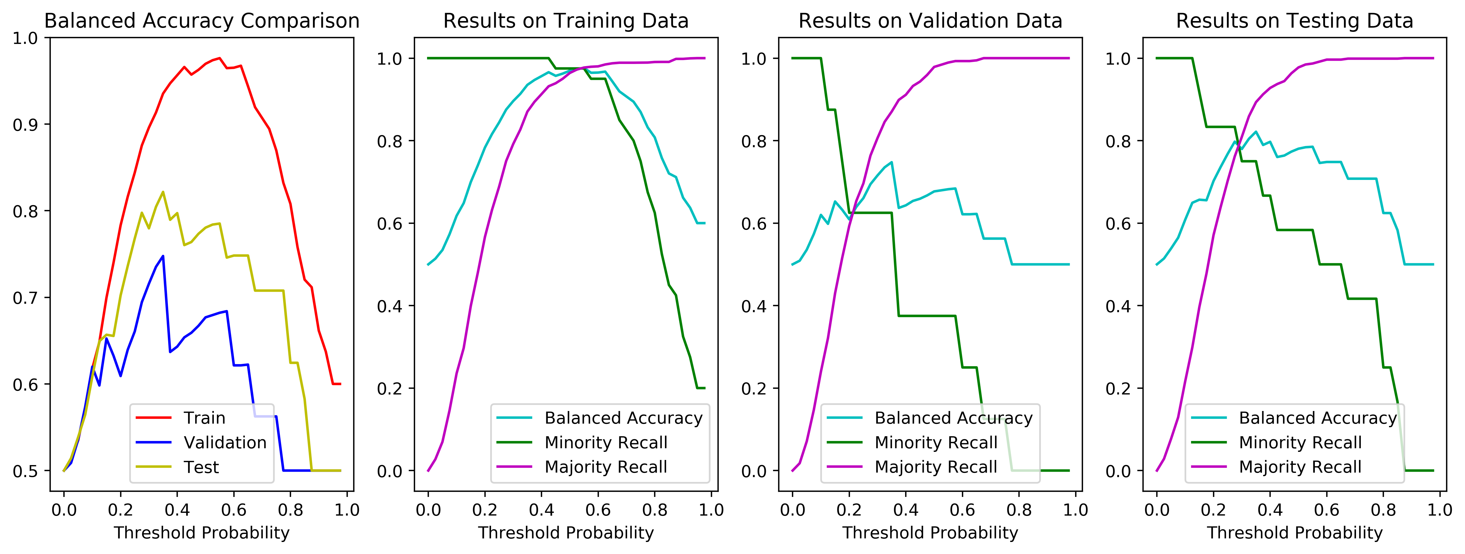
Figure 5: The performances of the proposed dynamic ensemble algorithm with respect to the change of the threshold parameter $\delta$ in Equation 20 on the UCI Bioassay dataset. Log likelihood is adopted to compute the likelihood of each test data.

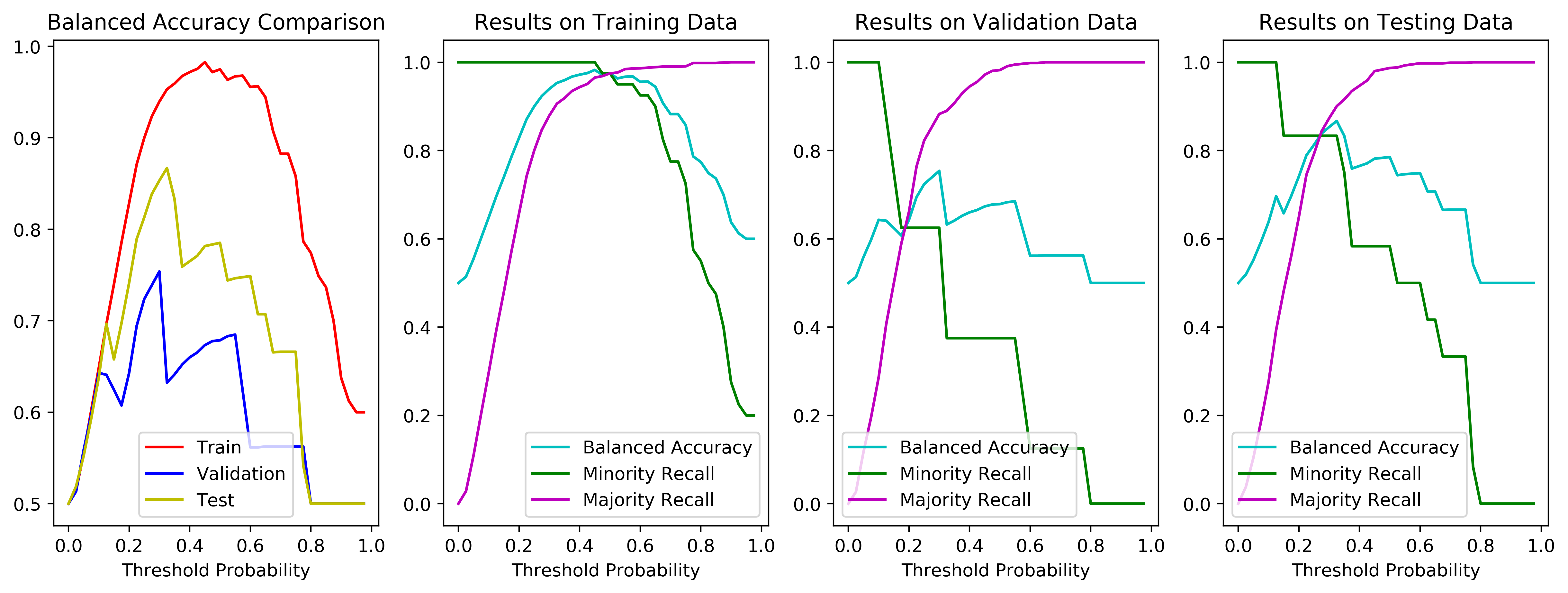
Figure 6: The performances of the proposed dynamic ensemble algorithm with respect to the change of the threshold parameter $\delta$ in Equation 20 on the UCI Bioassay dataset. Exponential likelihood is adopted to compute the likelihood of each test data.

The optimal $\delta$ value, based on the validation data, is $0.35$ for the log-likelihood AER, and $0.30$ for the exp-likelihood AER. The selection of the parameter shows that the overall algorithm favors spotting the majority instances over minority samples, as the optimal $\delta$ values under both settings are less than $0.5$. However, given the condition that the minority instances are sparse in the validation and test sets, the results are satisfactory. To provide some further insights, the statistics of the F1 score and G-Mean are given in Figures 7 and 8. The figures denote the change in the F1 score and G-mean metrics for different $\delta$ values with the log- and exp- likelihoods, respectively.

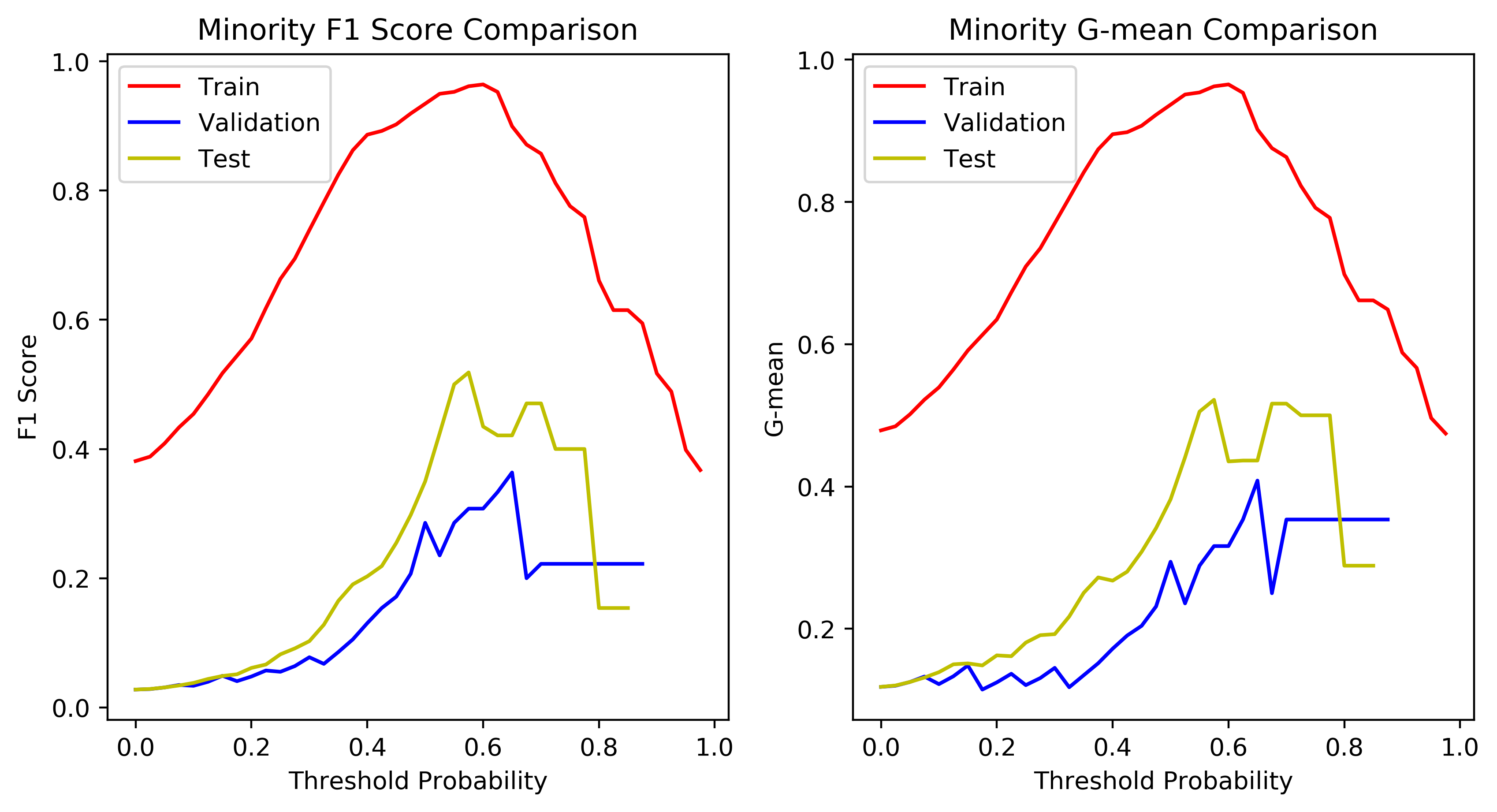
Figure 7: Change in $F_{1}$ score and G-mean of the minority data with respect to the changing value of $\delta$ in Equation 20 on the UCI Bioassay dataset. Log likelihood is adopted to compute the likelihood of each test data.

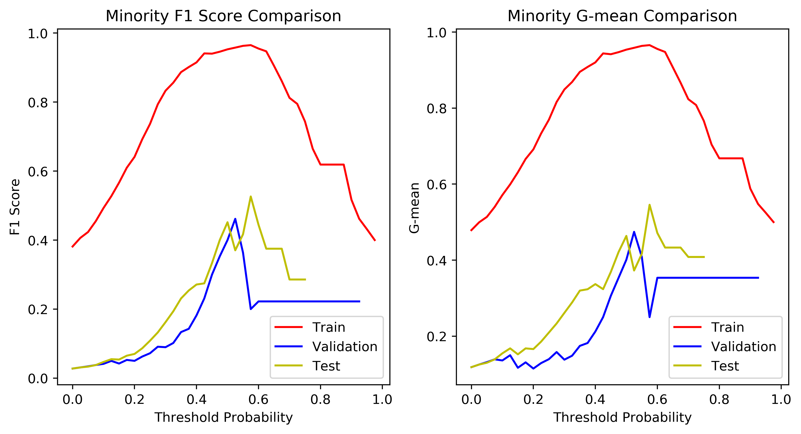
Figure 8: Change in $F_{1}$ score and G-mean of the minority data with respect to the changing value of $\delta$ in Equation 20 on the UCI Bioassay dataset. Exponential likelihood is adopted to compute the likelihood of each test data.

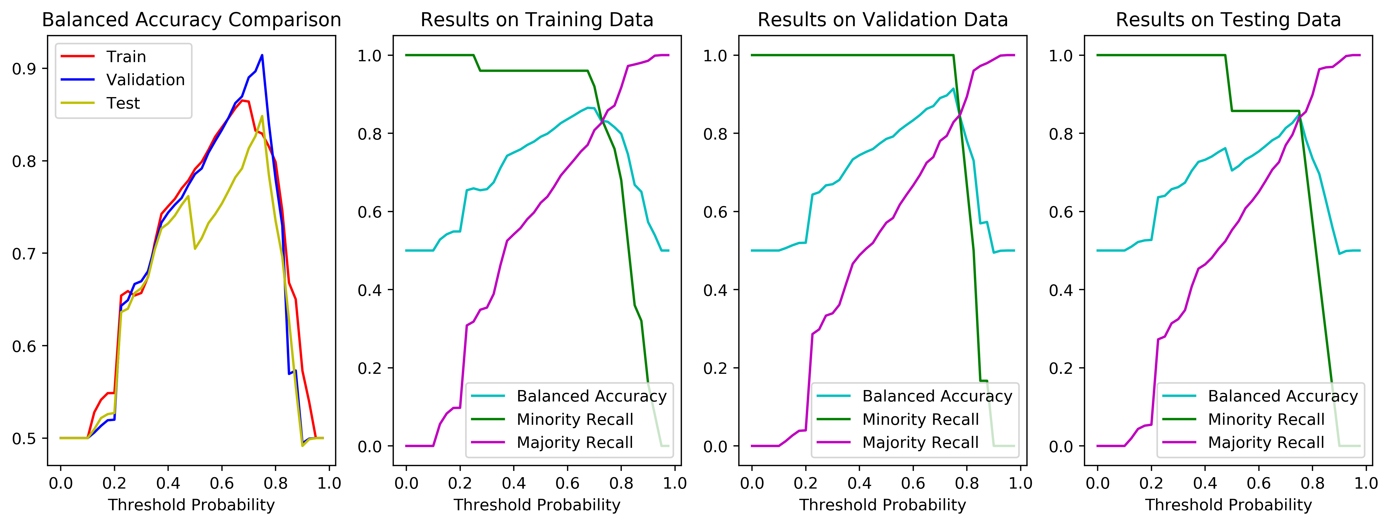
Figure 9: Performance of the proposed dynamic ensemble algorithm with respect to changes in the threshold parameter $\delta$ in Equation 20 on the Abalone 19 dataset. Log likelihood is adopted to compute the likelihood of each test data.

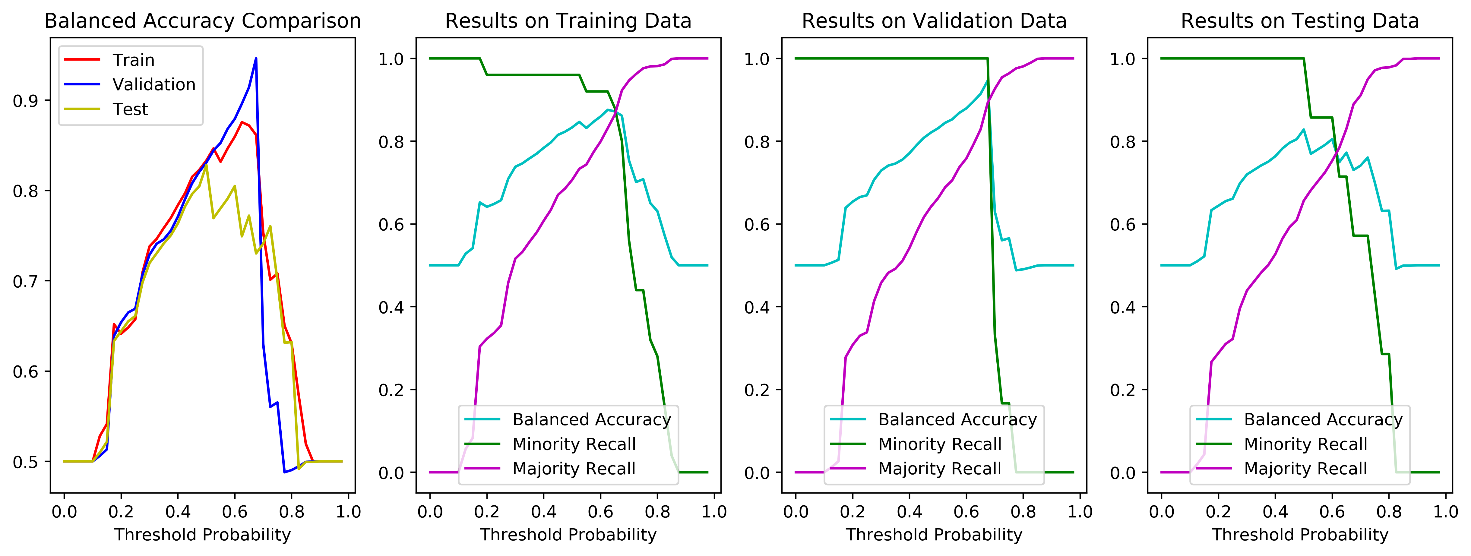
Figure 10: Performances of the proposed dynamic ensemble algorithm with respect to changes in the threshold parameter $\delta$ in Equation 20 on the Abalone 19 dataset. Exponential likelihood is adopted to compute the likelihood of each test data.

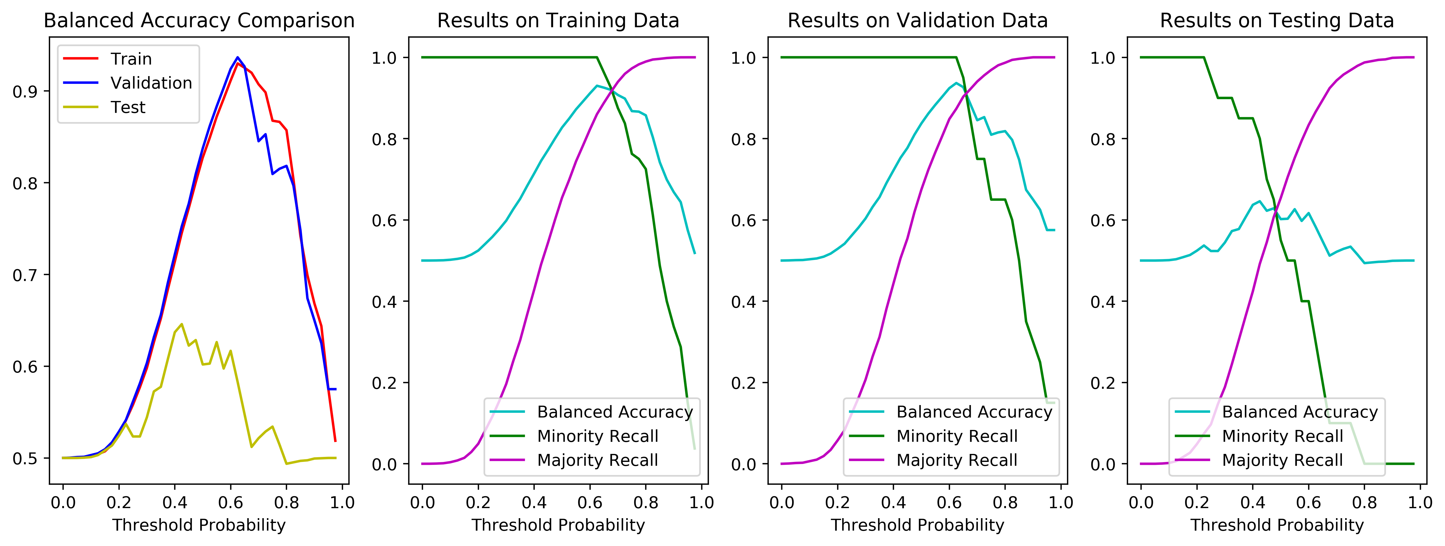
Figure 11: Performance of the proposed dynamic ensemble algorithm with respect to changes in the threshold parameter $\delta$ in Equation 20 on the GMM-generated dataset. Log likelihood is adopted to compute the likelihood of each test data.

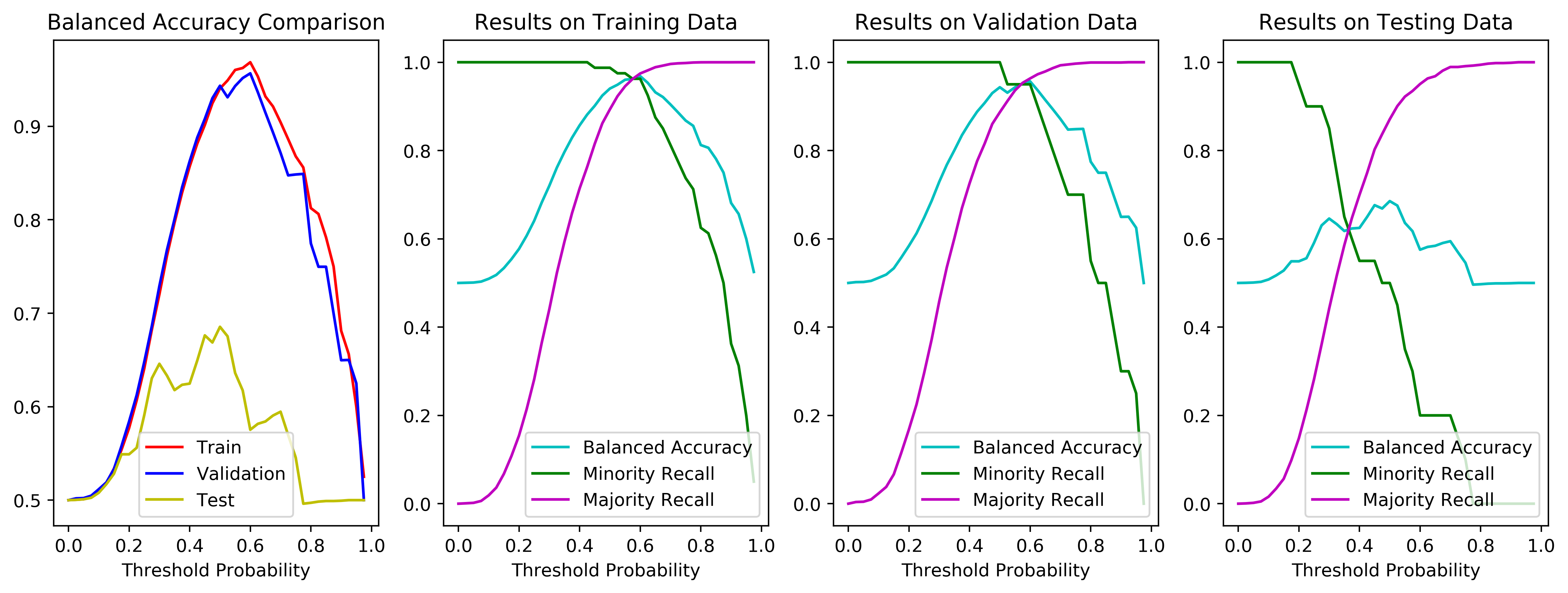
Figure 12: Performances of the proposed dynamic ensemble algorithm with respect to changes in the threshold parameter $\delta$ in Equation 20 on the GMM-generated dataset. Exponential likelihood is adopted to compute the likelihood of each test data.

Finally, Table 4 illustrates the performances of the comparison methods mentioned earlier and the AER-XGBoost method with both log- and exp-likelihoods. From Table 4, it can be observed that the AER-XGBoost algorithm yields a superior performance, based on multiple metrics. The exp-likelihood-based adaptive ensemble method can yield the best balanced accuracy, and its log-likelihood counterpart yields a better TP-FP ratio, because of a stronger capability in spotting majority instances. Among the compared methods, it can be observed that the focal loss neural network and LightGBM models cannot learn anything meaningful, and a plausible reason for this is that these models tend to overfit, especially when the dataset is small. The XGBoost and focal-XGBoost [17] demonstrate the strongest performance among the non-AER models. Nevertheless, we find that in the plot of the change in performance, with respect to $\delta$, the range of $\delta$ leading to a competent performance is quite restricted, which means its performance declines drastically, as $\delta$ is slightly larger/smaller than the desired range. This problem is much less significant in the AER models, as we can observe from Figures 5 and 6.

Table 4: Comparison between the performance of different algorithms on the UCI Bioassay dataset.

	Minority Recall	Majority Recall	TP-FP Ratio	F1 score	G-mean	Balanced Accuracy
Cost-sensitive SVM	75.00%	84.93%	5.0238	0.1224	0.2236	79.97%
Cost-sensitive Decision Tree	75.00%	85.16%	5.1048	0.1241	0.2253	80.08%
Focal loss neural network	0	100%	–	–	–	50.00%
LightGBM	0	100%	–	–	–	50.00%
Plain XGBoost	83.33%	0.47%	0.8373	0.0232	0.0990	41.90%
Focal-loss XGBoost	83.33%	78.19%	3.8225	0.0971	0.2073	80.77%
Dynamic Ensemble (log)	83.33%	0.47%	0.8373	0.0232	0.0990	41.90%
Dynamic Ensemble (exp)	83.33%	78.19%	3.8225	0.0971	0.2073	80.77%
AER-XGBoost (Log)	75.00%	89.34%	7.0333	0.1622	0.2611	82.16%
AER-XGBoost (Exp)	83.33%	87.33%	6.5732	0.1550	0.2668	85.33%

6.2 Abalone 19 Data

The candidate list of the number of Gaussian distributions for the Abalone 19 Dataset is set to $\{11,12,13\}$, and the number $12$ is retrieved through the BIC criteria. The optimal $\lambda$ is determined as $0.15$ for the log-likelihood, and $0.20$ for the exp-likelihood. Further, we again select the $\delta$ values that guarantee the optimal performance on the validation set as the “determined threshold.” The $\delta$ value AER models on the Abalone data is $0.75$ for the log-likelihood, and $0.675$ for the exp-likelihood. The performance, with respect to the changes in the $\delta$ values, is given in Figures 9 and 10.

All the methods mentioned in the previous experiment are implemented under the context of the Abalone 19 dataset. Because we no longer retrieve the performance from other literature, the decision tree model is implemented with the SK-learn CART decision tree (almost identical to C4.5 for classification problems), and the SVM model is fine-tuned using the best kernel among linear, RBF and Polynomial. The $\gamma$ parameter for the focal-XGBoost and the focal loss neural network are obtained via a validation grid search, and the final values are set to $2.5$ and $3.0$.

Table 5: The comparison between the performance of different algorithms on Abalone 19 dataset.

	Minority Recall	Majority Recall	TP-FP Ratio	F1 score	G-mean	Balanced Accuracy
Cost-sensitive SVM	28.57%	88.66%	2.5198	0.0388	0.0772	58.62%
Cost-sensitive Decision Tree	14.29%	99.64%	–	0.1818	0.1889	56.96%
Focal loss neural network	0	100%	–	–	–	50.00%
LightGBM	0	100%	–	–	–	50.00%
Plain XGBoost	100%	0.12%	1.0012	0.0166	0.0916	50.06%
Focal-loss XGBoost	42.86%	85.52%	2.9607	0.0462	0.1022	64.19%
Dynamic Ensemble (log)	57.14%	86.61%	4.2677	0.0656	0.1410	71.88%
Dynamic Ensemble (exp)	57.14%	86.61%	4.2677	0.0656	0.1410	71.88%
AER-XGBoost (Log)	85.71%	83.96%	5.3426	0.082	0.1924	84.83%
AER-XGBoost (Exp)	57.14%	88.90%	5.1491	0.0777	0.1543	73.02%

Table 5 reports the performances of the AER and the compared methods. From the table, it can be observed that the AER method (AER-XGBoost with both log- and exp-likelihoods) outperforms existing algorithms, in terms of the balanced accuracy and G-mean score on the Abalone 19 data. The AER-XGBoost with the exponential likelihood has a lower balanced accuracy, because of a relatively lower recall on minority instances; however, it is still higher than those of existing methods. On this dataset, the vanilla XGBoost, the focal loss neural network, and the LightGBM models all scramble to learn anything useful. The performances of the cost-sensitive SVM and decision tree are better than random guess, but still far from satisfactory. Once again, the focal-XGBoost exhibits a relatively competitive performance, although it is still inferior to the AER-XGBoost methods. It can be observed that the multiple entries in the table are given as ’-’; this is because one or more metrics of the method is out of the ordinary range, which results in ridiculously high/low or even inf or Nan results.

Table 6: McNemar’s test for Log- and Exp-likelihood AERs against existing methods on the Abalone 19 dataset($\alpha=0.05$)

. $\chi^{2}$ statistics $p$-value Null Hypothesis Log-likelihood AER Cost-sensitive Decision Tree 112.23 $<0.01$ Reject $H_{0}$ Cost-sensitive SVM 11.68 $<0.01$ Reject $H_{0}$ Focal loss neural network 114.2 $<0.01$ Reject $H_{0}$ LightGBM 114.2 $<0.01$ Reject $H_{0}$ Dynamic Ensemble (log) 9.5 $<0.01$ Reject $H_{0}$ Plain XGBoost 113.22 $<0.01$ Reject $H_{0}$ Focal XGBoost 0.68 $0.41$ Failed to reject $H_{0}$ Exp-likelihood AER Cost-sensitive Decision Tree 75.26 $<0.01$ Reject $H_{0}$ Cost-sensitive SVM 0.08 $0.77$ Failed to reject $H_{0}$ Focal loss neural network 114.2 $<0.01$ Reject $H_{0}$ LightGBM 114.2 $<0.01$ Reject $H_{0}$ Dynamic Ensemble (exp) 4.3 $0.04$ Reject $H_{0}$ Plain XGBoost 4.0 $<0.01$ Reject $H_{0}$ Focal XGBoost 54.0 $0.02$ Reject $H_{0}$

Table 7: Wilcoxon test for Log- and Exp-likelihood AERs against existing methods on the Abalone 19 dataset($\alpha=0.05$)

. $\chi^{2}$ statistics $p$-value Null Hypothesis Log-likelihood AER Cost-sensitive Decision Tree 274.0 $<0.01$ Reject $H_{0}$ Cost-sensitive SVM 4402.0 $0.15$ Failed to reject $H_{0}$ Focal loss neural network 0 $<0.01$ Reject $H_{0}$ Light GBM 0 $<0.01$ Reject $H_{0}$ Dynamic Ensemble (log) 136.5 $<0.01$ Reject $H_{0}$ Plain XGBoost 0 $<0.01$ Reject $H_{0}$ Focal XGBoost 3146.0 $0.14$ Failed to reject $H_{0}$ Exp-likelihood AER Cost-sensitive Decision Tree 188.0 $<0.01$ Reject $H_{0}$ Cost-sensitive SVM 2331.0 $0.01$ Reject $H_{0}$ Focal loss neural network 0 $<0.01$ Reject $H_{0}$ LightGBM 0 $<0.01$ Reject $H_{0}$ Dynamic Ensemble (exp) 1064.0 $0.03$ Reject $H_{0}$ Plain XGBoost 0 $<0.01$ Reject $H_{0}$ Focal XGBoost 3795.0 $0.02$ Reject $H_{0}$

Another interesting perspective offered by the table is the comparison between the vanilla XGBoost (the base classifier used in the AER method) and the advanced methods based on it (including the focal loss proposed in [17] and the AER method proposed in this study). It can be observed that the plain XGBoost method performs poorly at this specific task, with a significant bias toward the minority data, and failure at spotting the majority instances. The focal loss and AER can be regarded as two ·approaches to improving the performance, and the AER is superior, in terms of the overall performance.

Finally, Tables 6 and 7 demonstrate the results of the Mcnemar’s and Wilcoxon tests, to reveal the significance of the performance superiority of the AER models. From the tables, it can be observed that the preferable performances of the AER models are corroborated by both tests in most cases. The null hypothesis between the logarithm-based AER-XGBoost and the focal-loss XGBoost is relatively hard to reject ($p\geq 0.01$ for both tests), confirming the strong performance of the widely favored method. It is interesting that, for the SVM method, we failed to reject the null hypothesis for the exp-AER under the McNemar’s test and the log-AER under the Wilcoxon test. Such observations are not made elsewhere in the experiments. Thus, the problem in these specific datasets could stem from the specific training/testing split pairs.

6.3 GMM-generated Data and Variations

For the GMM-generated data, we first present the results on the $9$-center GMM-based set. For this model, the number of candidate Gaussian centroids is listed as $\{8,9,10\}$, and the $9$-centroid model is finally determined, which is consistent with the generative distribution of the data. The optimal $\lambda$ is determined as $0.60$ for the log-likelihood, and $0.30$ for the exp-likelihood. The validation set is selected to determine the value of $\delta$, and the performance, with respect to a varying $\delta$ value can be shown in Figures 11 and 12 for the log- and exp-likelihood methods respectively.

Similar to the previous experiments, the two types of the AER models and the methods of comparisons, including the cost-sensitive SVM and cost-sensitive decision tree, focal loss neural network, LightGBM, and the vanilla and focal-loss XGBoost models, are tested on the $9$-center GMM dataset. The results are summarized in Table 8. From the table, it can be found that only the cost-sensitive decision tree, focal-loss XGBoost, and the AER methods can grasp useful information, whereas other methods failed at learning more than some random classification boundaries. These results are consistent with what we have discussed earlier; the classification of the minority data is very hard to learn, because the 100 samples come from nine different Gaussian distributions. Nevertheless, with the AER methods, especially under the setup of the exp-likelihood, the model can maintain a relatively good performance. The results in Table 8 indicates that if the data manifold really conforms to the GMM, the AER-XGBoost method can serve as a powerful learner that extracts information from the highly complicated manifold, where most of the other models will fail.

Table 8: The comparison between the performance of different algorithms on the 9-center GMM-generated data.

	Minority Recall	Majority Recall	TP-FP Ratio	F1 score	G-mean	Balanced Accuracy
Cost-sensitive SVM	0%	100%	–	–	–	50.00%
Cost-sensitive Decision Tree	5.03%	99.18%	6.0769	0.0588	0.0598	52.09%
Focal loss neural network	0	100%	–	–	–	50.00%
LightGBM	0	100%	–	–	–	50.00%
Plain XGBoost	100%	0.063%	1.0006	–	–	50.03%
Focal-loss XGBoost	25.00%	84.49%	1.6122	0.0370	0.0707	54.74%
Dynamic Ensemble (log)	83.33%	0.47%	0.8373	0.0132	0.0195	48.35%
Dynamic Ensemble (exp)	83.33%	78.19%	3.8225	0.0132	0.0195	48.35%
AER-XGBoost (Log)	30.00%	86.58%	2.2358	0.0504	0.0909	58.29%
AER-XGBoost (Exp)	20.00%	95.06%	4.0513	0.0743	0.0988	57.53%

The results of the hypothetical test on $9$-center GMM data, together with the performances and the testing results on other variations of the GMM-generated data, are given in Table 9. From the table, it can be observed that the AER method consistently outperforms all the compared methods, with a considerable margin. Moreover, both statistical hypothesis tests support the significance of the performance superiority. The exp-likelihood-based AER performs better on the hypothesis tests, indicating that this type of AER method can distinguish its predictions from that of other models more effectively.

Table 9: Results on the GMM-generated datasets with different number of informative features.

	F1 Score	G-mean	Balanced Accuracy	(Wilcoxon)$H_{0}$ Log-AER-XGBoost	(Wilcoxon)$H_{0}$ Exp-AER-XGBoost	(Mcnemar)$H_{0}$ Log-AER-XGBoost	(Mcnemar)$H_{0}$ Exp-AER-XGBoost
Informative Feature Number $n_{\text{informative}}=8$
Cost-sensitive Decision Tree	0.0816	0.0830	54.15%	Reject	Reject	Reject	Reject
Cost-sensitive SVM	–	–	50.00%	Reject	Reject	Reject	Reject
Focal loss neural network	0.005	0.0625	50.00%	Reject	Reject	Reject	Reject
LightGBM	–	–	50.00%	Reject	Reject	Reject	Reject
Plain XGBoost	0.0693	0.1160	61.96%	Failed Reject	Reject	Failed Reject	Reject
Focal XGBoost	0.0344	0.1186	61.74%	Reject	Reject	Reject	Reject
Dynamic Ensemble (log)	0.0653	0.1193	63.13 %	Reject	–	Reject	–
Dynamic Ensemble (exp)	0.0653	0.1193	63.13 %	–	Reject	–	Reject
Log-AER-XGBoost	0.0707	0.1173	62.09%	–	–	–	–
Exp-AER-XGBoost	0.1159	0.1647	66.52%	–	–	–	–
Informative Feature Number $n_{\text{informative}}=9$
Cost-sensitive Decision Tree	0.0588	0.0598	52.09%	Reject	Reject	Reject	Reject
Cost-sensitive SVM	–	–	50.00%	Reject	Reject	Reject	Reject
Focal loss neural network	0.0114	0.0115	50.00%	Reject	Reject	Reject	Reject
LightGBM	–	–	50.00%	Reject	Reject	Reject	Reject
Plain XGBoost	–	–	50.03%	Reject	Reject	Reject	Reject
Focal XGBoost	0.0370	0.0707	54.74%	Reject	Reject	Failed Reject	Reject
Dynamic Ensemble (log)	0.0132	0.0195	48.39 %	Reject	–	Reject	–
Dynamic Ensemble (exp)	0.0132	0.0195	48.39 %	–	Reject	–	Reject
Log-AER-XGBoost	0.0504	0.0909	58.29%	–	–	–	–
Exp-AER-XGBoost	0.0743	0.0988	57.53%	–	–	–	–
Informative Feature Number $n_{\text{informative}}=10$
Cost-sensitive Decision Tree	0.1176	0.1195	54.62%	Reject	Reject	Reject	Reject
Cost-sensitive SVM	–	–	50.00%	Reject	Reject	Reject	Reject
Focal loss neural network	0.0179	0.0198	50.00%	Reject	Reject	Reject	Reject
LightGBM	0.0952	0.2236	50.00%	Reject	Reject	Reject	Reject
Plain XGBoost	0.0629	0.0948	58.26%	Failed Reject	Reject	Failed Reject	Reject
Focal XGBoost	0.1091	0.1134	56.49%	Reject	Failed Reject	Reject	Failed Reject
Dynamic Ensemble (log)	0.0596	0.1067	60.92 %	Reject	–	Reject	–
Dynamic Ensemble (exp)	0.0596	0.1067	60.92 %	–	Reject	–	Reject
Log-AER-XGBoost	0.1032	0.1540	65.98%	–	–	–	–
Exp-AER-XGBoost	0.1684	0.2066	67.88%	–	–	–	–
Informative Feature Number $n_{\text{informative}}=11$
Cost-sensitive Decision Tree	–	0.0	49.36%	Reject	Reject	Reject	Reject
Cost-sensitive SVM	–	–	50.00%	Reject	Reject	Reject	Reject
Focal loss neural network	0.0146	0.0148	50.00%	Reject	Reject	Reject	Reject
LightGBM	–	–	50.00%	Reject	Reject	Reject	Reject
Plain XGBoost	0.0397	0.0586	53.44%	Reject	Reject	Reject	Reject
Focal XGBoost	0.0388	0.0656	54.24%	Failed Reject	Reject	Failed Reject	Reject
Dynamic Ensemble (log)	0.0690	0.1	58.70 %	Reject	–	Reject	–
Dynamic Ensemble (exp)	0.0448	0.0785	56.23 %	–	Reject	–	Reject
Log-AER-XGBoost	0.0863	0.1230	61.42%	–	–	–	–
Exp-AER-XGBoost	0.1522	0.1845	65.44%	–	–	–	–
Informative Feature Number $n_{\text{informative}}=12$
Cost-sensitive Decision Tree	–	0.00	49.43%	Reject	Reject	Reject	Reject
Cost-sensitive SVM	–	–	50.00%	Reject	Reject	Reject	Reject
Cost-sensitive Network	0.0128	0.0128	50.00%	Reject	Reject	Reject	Reject
LightGBM	–	–	50.00%	Reject	Reject	Reject	Reject
Plain XGBoost	0.0410	0.0747	55.57%	Reject	Reject	Reject	Reject
Focal XGBoost	0.0800	0.1000	52.37%	Reject	Reject	Reject	Reject
Dynamic Ensemble (log)	0.0339	0.0452	51.96 %	Reject	–	Failed Reject	–
Dynamic Ensemble (exp)	0.0516	0.0770	55.85 %	–	Failed Reject	–	Failed Reject
Log-AER-XGBoost	0.0662	0.0977	58.51%	–	–	–	–
Exp-AER-XGBoost	0.1687	0.1972	65.72%	–	–	–	–

6.4 Other UCI Imbalanced Datasets

Tables 10-24 show the results of performance and statistical hypothesis tests for five other UCI datasets, namely Ecoli, US Crime, Wine Quality, Scene, and Car Eval. The characteristics of these datasets have been discussed in Section 5.1 and Table 2. It can be observed that, compared with the three datasets we discussed earlier, these five datasets have considerably less imbalanced ratio. Therefore, the advantages of the AER-XGBoost model in this context are not as significant as in the above experiments. Nevertheless, they can still serve as powerful proofs of the effectiveness of the AER models.

Tables 10-12 illustrate the performances and the results of the statistical tests on the Ecoli data. From the tables, it can be found that the AER model does not outperform the recent novel methods (e.g. Light GBM, XGBoost, and focal-XGBoost), although it is better than the conventional algorithms (e.g. SVM and decision tree). The inadequacy of the performance can be partially explained by the lower imbalance rate, which compromises the AER’s specialization in processing imbalanced data, and prompts some recent general-purpose methods to unleash their abilities in handling ordinary datasets. Regardless of the performances in comparison to the other methods, the comparison with pure dynamic ensemble still validates the effectiveness of the AER framework. Furthermore, both types of statistical hypothesis tests suggest that the difference between the prediction of the AER-XGBoost and other methods is significant, to reject the null hypothesis in most of the cases.

Table 10: The comparison between the performance of different algorithms on the Ecoli data.

	Minority Recall	Majority Recall	TP-FP Ratio	F1 score	G-mean	Balanced Accuracy
Cost-sensitive SVM	75%	92.19%	9.6	0.5	0.5303	83.59%
Cost-sensitive Decision Tree	50%	98.44%	32.0	0.5714	0.5774	74.22%
Focal loss neural network	0	100%	–	–	–	50.00%
LightGBM	75.00%	98.44%	48.0	0.75	0.75	86.72%
XGBoost	100%	84.38%	6.4	0.4444	0.5345	92.19%
Focal-loss XGBoost	75.00%	98.44%	48.0	0.75	0.75	86.72%
Dynamic Ensemble (Log)	75.00%	92.19%	9.6	0.5	0.5303	83.59%
Dynamic Ensemble (Exp)	75.00%	85.94%	5.3	0.375	0.433	80.47%
AER-XGBoost (Log)	75.00%	92.19%	9.6	0.5	0.5303	83.59%
AER-XGBoost (Exp)	75.00%	93.75%	12.0	0.5455	0.5669	84.38%

Table 11: McNemar’s test for Log- and Exp-likelihood AERs against existing methods on the Ecoli dataset($\alpha=0.05$)

. $\chi^{2}$ statistics $p$-value Null Hypothesis Log-likelihood AER Cost-sensitive Decision Tree 4.17 $<0.01$ Reject $H_{0}$ Cost-sensitive SVM 0.5 $0.48$ Failed to Reject $H_{0}$ Focal loss neural network 4.17 $<0.01$ Reject $H_{0}$ LightGBM 4.17 $<0.01$ Reject $H_{0}$ Plain XGBoost 0.8 $0.37$ Failed to Reject $H_{0}$ Focal XGBoost 4.17 $<0.01$ Reject $H_{0}$ Dynamic Ensemble (log) 0.0 1.0 Failed to Reject $H_{0}$ Exp-likelihood AER Cost-sensitive Decision Tree 19.36 $<0.01$ Reject $H_{0}$ Cost-sensitive SVM 15.43 $<0.01$ Reject $H_{0}$ Focal loss neural network 4.17 $<0.01$ Reject $H_{0}$ LightGBM 4.17 $<0.01$ Reject $H_{0}$ Plain XGBoost 12.07 $<0.01$ Reject $H_{0}$ Focal XGBoost 19.36 $<0.01$ Reject $H_{0}$ Dynamic Ensemble (exp) 11.53 $<0.01$ Reject $H_{0}$

Table 12: Wilcoxon test for Log- and Exp-likelihood AERs against existing methods on the Ecoli dataset($\alpha=0.05$)

. $\chi^{2}$ statistics $p$-value Null Hypothesis Log-likelihood AER Cost-sensitive Decision Tree 0 $0.01$ Reject $H_{0}$ Cost-sensitive SVM 0 $0.16$ Failed to reject $H_{0}$ Focal loss neural network 0 $0.01$ Reject $H_{0}$ Light GBM 0 $0.01$ Reject $H_{0}$ Plain XGBoost 0 $0.02$ Reject $H_{0}$ Focal XGBoost 0 $0.01$ Reject $H_{0}$ Dynamic Ensemble (log) 6.0 $0.65$ Failed to reject $H_{0}$ Exp-likelihood AER Cost-sensitive Decision Tree 0 $<0.01$ Reject $H_{0}$ Cost-sensitive SVM 0 $<0.01$ Reject $H_{0}$ Focal loss neural network 0 $<0.01$ Reject $H_{0}$ Light GBM 0 $<0.01$ Reject $H_{0}$ Plain XGBoost 0 $<0.01$ Reject $H_{0}$ Focal XGBoost 0 $<0.01$ Reject $H_{0}$ Dynamic Ensemble (exp) 0 $<0.01$ Reject $H_{0}$

Tables 13-15 demonstrate the experimental results on the US Crime data. The performances in Table 13 further demonstrate the advantages of the AER models, which outperform the classical models (SVM and decision tree) by a large margin, and achieve better scores than recent models such as the LightGBM, XGBoost and focal-XGBoost. The comparisons of the AER models with their pure likelihood-based (unregularized) counterparts also demonstrate the effectiveness of the regularization property. Furthermore, Tables 14 and 15 show the results of the hypothesis tests. Both tests suggest that the upper-hand performance superiority of the exponential-based AER-XGBoost is deemed significant. The logarithm-based AER-XGBoost performs relatively badly on the Mcnamar’s test; however, the same results on the Wilcoxon test are mostly positive, suggesting that the failure of the Mcnamar’s test can be attributed to the nature of the dataset.

Table 13: The comparison between the performance of different algorithms on the US Crime data.

	Minority Recall	Majority Recall	TP-FP Ratio	F1 score	G-mean	Balanced Accuracy
Cost-sensitive SVM	42.86%	94.71%	8.1	0.36	0.3647	68.78%
Cost-sensitive Decision Tree	42.86%	96.83%	13.5	0.4286	0.4286	69.84%
Focal loss neural network	1.75%	98.25%	1.0	0.0263	0.0304	50.00%
LightGBM	28.57%	98.68%	21.60	0.3750	0.3948	63.62%
XGBoost	57.14%	94.71%	10.8	0.4528	0.4629	75.93%
Focal-loss XGBoost	57.14%	94.44%	10.3	0.4444	0.4558	75.79%
Dynamic Ensemble (Log)	71.43%	91.53%	8.4	0.4412	0.4775	81.48%
Dynamic Ensemble (Exp)	90.48%	85.45%	6.2	0.4	0.4820	87.96%
AER-XGBoost (Log)	71.437%	91.80%	8.7	0.4478	0.4826	81.61%
AER-XGBoost (Exp)	90.48%	87.83%	7.4	0.4419	0.5143	89.15%

Table 14: McNemar’s test for Log- and Exp-likelihood AERs against existing methods on the US Crime dataset($\alpha=0.05$)

. $\chi^{2}$ statistics $p$-value Null Hypothesis Log-likelihood AER Cost-sensitive Decision Tree 1.64 $0.2$ Failed to Reject $H_{0}$ Cost-sensitive SVM 0.59 $0.44$ Failed to Reject $H_{0}$ Focal loss neural network 6.92 $<0.01$ Reject $H_{0}$ LightGBM 6.92 $<0.01$ Reject $H_{0}$ Plain XGBoost 2.27 $0.14$ Failed to Reject $H_{0}$ Focal XGBoost 1.71 $0.19$ Failed to Reject $H_{0}$ Dynamic Ensemble (log) 0.14 0.71 Failed to Reject $H_{0}$ Exp-likelihood AER Cost-sensitive Decision Tree 236.9 $<0.01$ Reject $H_{0}$ Cost-sensitive SVM 236.2 $<0.01$ Reject $H_{0}$ Focal loss neural network 0.64 $0.42$ Failed to Reject $H_{0}$ LightGBM 0.64 $0.42$ Failed to Reject $H_{0}$ Plain XGBoost 246.0 $<0.01$ Reject $H_{0}$ Focal XGBoost 245.0 $<0.01$ Reject $H_{0}$ Dynamic Ensemble (exp) 241.3 $<0.01$ Reject $H_{0}$

Table 15: Wilcoxon test for Log- and Exp-likelihood AERs against existing methods on the US Crime dataset($\alpha=0.05$)

. $\chi^{2}$ statistics $p$-value Null Hypothesis Log-likelihood AER Cost-sensitive Decision Tree 115.0 $0.67$ Failed to Reject $H_{0}$ Cost-sensitive SVM 47.5 $0.06$ Failed to Reject $H_{0}$ Focal loss neural network 7.5 $<0.01$ Reject $H_{0}$ Light GBM 7.5 $<0.01$ Reject $H_{0}$ Plain XGBoost 55.0 $0.02$ Reject $H_{0}$ Focal XGBoost 42.0 $<0.01$ Reject $H_{0}$ Dynamic Ensemble (log) 107.5 $<0.01$ Reject $H_{0}$ Exp-likelihood AER Cost-sensitiveDecision Tree 294.0 $<0.01$ Reject $H_{0}$ Cost-sensitive SVM 0 $<0.01$ Reject $H_{0}$ Focal loss neural network 0 $<0.01$ Reject $H_{0}$ Light GBM 0 $<0.01$ Reject $H_{0}$ Plain XGBoost 0 $<0.01$ Reject $H_{0}$ Focal XGBoost 0 $<0.01$ Reject $H_{0}$ Dynamic Ensemble (exp) 0 $<0.01$ Reject $H_{0}$

The third dataset we tested the models on is the famous Wine Quality dataset, and the results are presented in Tables 16-18. From Table 16, it can be observed that apart from the classical methods (SVM and decision tree), the performance of the AER is roughly in the same range as those of the other recent and advanced models. One exception is the focal-XGBoost, which scores $81.75\%$ in terms of balanced accuracy. However, this score can be attributed to the fact that it compromises the classification of the majority data, which also leads to lower F1 and G-mean scores. In addition to the performances, the results in Table 17 suggest that the Mcnemar’s tests reject the Null hypothesis for all but three models, namely the cost-sensitive decision trees, focal loss neural network, and LightGBM. It may be observed that the results of the focal loss neural network and LightGBM are almost “all-majority” prediction; therefore, we can safely conclude that the failure of rejection is attributable to the imbalanced nature of the dataset. Furthermore, the results in Table 18 suggest the Wilcoxon tests reject almost all the null hypotheses.

Table 16: The comparison between the performance of different algorithms on the Wine Quality data.

	Minority Recall	Majority Recall	TP-FP Ratio	F1 score	G-mean	Balanced Accuracy
Cost-sensitive SVM	60%	81.26%	3.2	0.1593	0.2347	70.63%
Cost-sensitive Decision Tree	23.33%	98.32%	13.85	0.2642	0.2665	60.82%
Focal loss neural network	1.94%	98.06%	1.0	0.0237	0.0244	50.00%
LightGBM	10.00%	99.37%	15.83	0.1538	0.1826	54.68%
XGBoost	60%	92.21%	7.7	0.2951	0.3426	76.11%
Focal-loss XGBoost	76.67%	86.84%	5.83	0.2584	0.3452	81.75%
Dynamic Ensemble (Log)	56.67%	92.00%	7.1	0.2764	0.3218	74.33%
Dynamic Ensemble (Exp)	60%	88.42%	5.2	0.2278	0.2904	74.21%
AER-XGBoost (Log)	56.67%	91.89%	7.0	0.2742	0.3201	74.28%
AER-XGBoost (Exp)	66.67%	91.05%	7.5	0.2963	0.3563	78.86%

Table 17: McNemar’s test for Log- and Exp-likelihood AERs against existing methods on the Wine Quality dataset($\alpha=0.05$)

. $\chi^{2}$ statistics $p$-value Null Hypothesis Log-likelihood AER Cost-sensitive Decision Tree 0.13 $0.72$ Failed to Reject $H_{0}$ Cost-sensitive SVM 133.0 $<0.01$ Reject $H_{0}$ Focal loss neural network 0.24 $0.63$ Failed to Reject $H_{0}$ LightGBM 0.24 0.63 Failed to Reject $H_{0}$ Plain XGBoost 33.3 $<0.01$ Reject $H_{0}$ Focal XGBoost 68.4 $<0.01$ Reject $H_{0}$ Dynamic Ensemble (log) 5.6 $0.01$ Reject $H_{0}$ Exp-likelihood AER Cost-sensitive Decision Tree 3.52 0.06 Failed to Reject $H_{0}$ Cost-sensitive SVM 116.3 $<0.01$ Reject $H_{0}$ Focal loss neural network 0.24 $0.63$ Failed to Reject $H_{0}$ LightGBM 0.24 0.63 Failed to Reject $H_{0}$ Plain XGBoost 14.0 $<0.01$ Reject $H_{0}$ Focal XGBoost 53.8 $<0.01$ Reject $H_{0}$ Dynamic Ensemble (exp) 55.7 $<0.01$ Reject $H_{0}$

Table 18: Wilcoxon test for Log- and Exp-likelihood AERs against existing methods on the Wine Quality dataset($\alpha=0.05$)

. $\chi^{2}$ statistics $p$-value Null Hypothesis Log-likelihood AER Cost-sensitive Decision Tree 240.0 $0.86$ Failed to Reject $H_{0}$ Cost-sensitive SVM 88.5 $<0.01$ Reject $H_{0}$ Focal loss neural network 18.0 $<0.01$ Reject $H_{0}$ Light GBM 18.0 $<0.01$ Reject $H_{0}$ Plain XGBoost 36. $<0.01$ Reject $H_{0}$ Focal XGBoost 199.5 $<0.01$ Reject $H_{0}$ Dynamic Ensemble (log) 126.0 $<0.01$ Reject $H_{0}$ Exp-likelihood AER Cost-sensitive Decision Tree 318.5 $<0.01$ Reject $H_{0}$ Cost-sensitive SVM 320.0 $<0.01$ Reject $H_{0}$ Focal loss neural network 19.5 $<0.01$ Reject $H_{0}$ Light GBM 19.5 $<0.01$ Reject $H_{0}$ Plain XGBoost 481.0 $<0.01$ Reject $H_{0}$ Focal XGBoost 285.0 $<0.01$ Reject $H_{0}$ Dynamic Ensemble(exp) 0 $<0.01$ Reject $H_{0}$

Th Scene dataset, as mentioned earlier, has richer information, with a greater number of features. The results in Table 19 reveal that the advantages of the AER model are more compelling in this type of scenario. We can observe from the table that the performance of AER-XGBoosts is significantly better than that of the other models, including the classical ones and the recently developed ones. Once more, the vanilla and focal XGBoost models yield relatively more satisfactory performances, as they are the only models that can compete against the AER models. The improvements in the performance of the AER over the pure dynamic ensemble further demonstrates the positive impact of regularization on the dynamic ensemble, especially when the data information is rich. Additionally, the results in Tables 20 and 21 give valid statistical testing results.

Table 19: The comparison between the performance of different algorithms on the Scene data.

	Minority Recall	Majority Recall	TP-FP Ratio	F1 score	G-mean	Balanced Accuracy
Cost-sensitive SVM	26.67%	96.24%	7.1	0.2909	0.2921	61.45%
Cost-sensitive Decision Tree	20.00%	91.59%	2.38	0.1622	0.1651	55.80%
Focal loss neural network	0%	100%	–	–	–	50.00%
LightGBM	3.33%	100%	–	0.0645	0.1826	51.67%
XGBoost	66.67%	72.35%	2.4	0.2286	0.3032	69.51%
Focal-loss XGBoost	66.67%	73.23%	2.5	0.2339	0.3075	66.95%
Dynamic Ensemble (Log)	43.33%	91.37%	5.02	0.3171	0.3291	67.35%
Dynamic Ensemble (Exp)	83.33%	41.15%	1.4	0.1558	0.2676	62.24%
AER-XGBoost (Log)	53.33%	89.82%	5.2	0.3478	0.3710	71.58%
AER-XGBoost (Exp)	66.67%	76.33%	2.8	0.2548	0.3240	71.50%

Table 20: McNemar’s test for Log- and Exp-likelihood AERs against existing methods on the Scene dataset($\alpha=0.05$)

. $\chi^{2}$ statistics $p$-value Null Hypothesis Log-likelihood AER Cost-sensitive Decision Tree 96.9 $<0.01$ Reject $H_{0}$ Cost-sensitive SVM 114.3 $<0.01$ Reject $H_{0}$ Focal loss neural network 116.8 $<0.01$ Reject $H_{0}$ LightGBM 116.8 $<0.01$ Reject $H_{0}$ Plain XGBoost 16.5 $<0.01$ Reject $H_{0}$ Focal XGBoost 61.8 $<0.01$ Reject $H_{0}$ Dynamic Ensemble (log) 0.5 $0.46$ Failed to Reject $H_{0}$ Exp-likelihood AER Cost-sensitive Decision Tree 242.3 $<0.01$ Reject $H_{0}$ Cost-sensitive SVM 228.0 $<0.01$ Reject $H_{0}$ Focal loss neural network 116.8 $<0.01$ Reject $H_{0}$ LightGBM 116.8 $<0.01$ Reject $H_{0}$ Plain XGBoost 151.2 $<0.01$ Reject $H_{0}$ Focal XGBoost 119.7 $<0.01$ Reject $H_{0}$ Dynamic Ensemble (exp) 32.6 $<0.01$ Reject $H_{0}$

Table 21: Wilcoxon test for Log- and Exp-likelihood AERs against existing methods on Scene dataset($\alpha=0.05$)

. $\chi^{2}$ statistics $p$-value Null Hypothesis Log-likelihood AER Cost-sensitive Decision Tree 756.0 $<0.01$ Reject $H_{0}$ Cost-sensitive SVM 227.5 $<0.01$ Reject $H_{0}$ Focal loss neural network 0 $<0.01$ Reject $H_{0}$ Light GBM 0 $<0.01$ Reject $H_{0}$ Plain XGBoost 1274.0 $<0.01$ Reject $H_{0}$ Focal XGBoost 1008.0 $<0.01$ Reject $H_{0}$ Dynamic Ensemble (log) 1820.0 $<0.29$ Failed to Reject $H_{0}$ Exp-likelihood AER Cost-sensitive Decision Tree 474.0 $<0.01$ Reject $H_{0}$ Cost-sensitive SVM 320.0 $<0.01$ Reject $H_{0}$ Focal loss neural network 0 $<0.01$ Reject $H_{0}$ Light GBM 0 $<0.01$ Reject $H_{0}$ Plain XGBoost 796.0 $<0.01$ Reject $H_{0}$ Focal XGBoost 388.5 $<0.01$ Reject $H_{0}$ Dynamic Ensemble(exp) 264.0 $<0.01$ Reject $H_{0}$

Finally, Tables 22-24 present the performances and results of the statistical tests on the Car Eval dataset. It can be observed that, as the dataset is relatively easy to learn (small size and low imbalance rate), almost all the models can yield good performance. Nevertheless, the AER-based models still yield better overall performances. It is also noticeable that, because the dataset is small, the dynamic ensemble without regularization can only offer performances comparable with classical methods, and the performances increase drastically after the introduction of regularization. In addition, the results of the hypothesis tests in Tables 23 and 24 suggest the differences in the predictions are significant.

Table 22: Comparison between the performance of different algorithms on the Car Eval data.

	Minority Recall	Majority Recall	TP-FP Ratio	F1 score	G-mean	Balanced Accuracy
Cost-sensitive SVM	89.29%	97.48%	35.5	0.8197	0.8224	93.38%
Cost-sensitive Decision Tree	82.14%	95.28%	17.4	0.6970	0.7051	88.71%
Focal loss neural network	0	100%	–	–	–	50.00%
LightGBM	92.86%	97.17%	32.8	0.8254	0.8305	95.01%
XGBoost	100%	88.68%	8.8	0.6087	0.6614	94.34%
Focal-loss XGBoost	100%	87.42%	8.0	0.5833	0.6417	93.71%
Dynamic Ensemble (Log)	96.43%	97.17%	34.1	0.8438	0.8504	96.80%
Dynamic Ensemble (Exp)	92.86%	95.91%	22.7	0.7761	0.7868	94.38%
AER-XGBoost (Log)	92.88%	97.17%	32.8	0.8254	0.8305	95.01%
AER-XGBoost (Exp)	100%	95.91%	24.5	0.8116	0.8264	97.96%

Table 23: McNemar’s test for Log- and Exp-likelihood AERs against existing methods on the Car Eval dataset($\alpha=0.05$)

. $\chi^{2}$ statistics $p$-value Null Hypothesis Log-likelihood AER Cost-sensitive Decision Tree 4.1 $<0.01$ Reject $H_{0}$ Cost-sensitive SVM 13.0 $<0.01$ Reject $H_{0}$ Focal loss neural network 14.1 $<0.01$ Reject $H_{0}$ LightGBM 14.1 $<0.01$ Reject $H_{0}$ Plain XGBoost 1.8 $0.18$ Failed to Reject $H_{0}$ Focal XGBoost 3.4 $0.07$ Failed to Reject $H_{0}$ Dynamic Ensemble(log) 8.5 $<0.01$ Reject $H_{0}$ Exp-likelihood AER Cost-sensitive Decision Tree 325.1 $<0.01$ Reject $H_{0}$ Cost-sensitive SVM 312.2 $<0.01$ Reject $H_{0}$ Focal loss neural network 14.1 $<0.01$ Reject $H_{0}$ LightGBM 14.1 $<0.01$ Reject $H_{0}$ Plain XGBoost 304.0 $<0.01$ Reject $H_{0}$ Focal XGBoost 300.0 $<0.01$ Reject $H_{0}$ Dynamic Ensemble(exp) 321.1 $<0.01$ Reject $H_{0}$

Table 24: Wilcoxon test for Log- and Exp-likelihood AERs against existing methods on the Car Eval dataset($\alpha=0.05$)

. $\chi^{2}$ statistics $p$-value Null Hypothesis Log-likelihood AER Cost-sensitive Decision Tree 0 $<0.01$ Reject $H_{0}$ Cost-sensitive SVM 0 $<0.01$ Reject $H_{0}$ Focal loss neural network 0 $<0.01$ Reject $H_{0}$ Light GBM 0 $<0.01$ Reject $H_{0}$ Plain XGBoost 30.0 $0.11$ Failed to Reject $H_{0}$ Focal XGBoost 87.5 $<0.01$ Reject $H_{0}$ Dynamic Ensemble(exp) 0 $<0.01$ Reject $H_{0}$ Exp-likelihood AER Cost-sensitive Decision Tree 0 $<0.01$ Reject $H_{0}$ Cost-sensitive SVM 0 $<0.01$ Reject $H_{0}$ Focal loss neural network 0 $<0.01$ Reject $H_{0}$ Light GBM 0 $<0.01$ Reject $H_{0}$ Plain XGBoost 0 $<0.01$ Reject $H_{0}$ Focal XGBoost 0 $<0.01$ Reject $H_{0}$ Dynamic Ensemble(exp) 0 $<0.01$ Reject $H_{0}$

7 Discussions

We dedicate this section to discussing the implications of the foregoing theoretical and empirical analysis and the missing details in the experiments. Specifically, we want to discuss the following aspects: 1. The effectiveness of the regularization; 2. The suitable problem for the AER and the choice between logarithm- and exponential-based AERs; 3. The practical training time and training dynamics of the AER; and 4. Natural improvements and extensions of the AER.

From the experiments in Section 6, it can be observed that the AER-XGBoost models (with regularization) almost always outperform their pure dynamic ensemble counterparts in terms of the balanced accuracy. The only notable exceptions are in Tables 5 and 8, where the unregularized exp-based dynamic ensemble models achieve much better balanced accuracy. However, this “performance flux” is at the cost of the majority recall, which results in low TP-FP ratios, and renders the models practically inapplicable. Furthermore, for most of the statistical hypothesis tests, the regularized AER-XGBoosts reject the prediction null hypothesis from their pure dynamic ensemble counterparts. For the UCI Bioassay data, from Figures 3 and 4, it can be observed that the optimal $\lambda$ for the validation and testing sets is neither $0$ nor $1$, indicating that interpolating the likelihood-based weights resulted in performance gain. The results on Abalone 19 and the GMM-generated data reveal similar results, which can further support the above observation.

As we have discussed based on the experiments, the AER is best suitable for problems with complex decision boundary and high imbalanced ratio. For instance, the performance of the AER-XGBoost only offers competitive performances on the Ecoli dataset (imbalance ratio $1:8.6$), whereas it offers significantly state-of-the-art performances on the Abalone 19 data (imbalance ratio $1:129$). Furthermore, from the observations, based on most of the experiments, the exponential likelihood-based AERs are often the better ones. We believe this may be attributable to the fact that they can benefit more from regularization. This can be explained by the fact that the logarithm-based AERs have weights closer to uniform, whereas the weights of the exponential-based AERs distribute more “sharply.” The major drawback of the exponential-based AER, compared with the logarithm-based one, is that the range of choice for the “good” hyper-parameters is smaller. Thus, we recommend using the logarithm-based AER models when we have no knowledge of the relations between the training/validation and the test data, and using the exponential-based AER when we know the data distribution between the training/validation and the test sets are similar.

We theoretically proved in Section 4 that the time and memory complexity of the models implemented under the AER framework is better than the vanilla framework. In practice, we observe that the running time for the AER-XGBoost is usually longer than expected. This can be explained by two factors. The first factor is that the time complexity of the XGBoost does not fall into the regime of polynomial time. Because the model includes parallelization during fitting, the complexity introduced by the number of data becomes $O(\log(m))$ (polylog) instead. In practice, we do not expect this type of classifier very often, and if the parallelization technique is enabled, we can also bring the GMM to parallel computing, to further improve the time complexity. The second factor is that we do not implement diagonal approximations for the co-variance matrices in the GMM models. Therefore, it takes $O(n^{3})$ complexity to compute the matrix inverse and multiplications (in contrast with the $O(n)$ complexity using diagonal approximation). We employed full co-variance matrices to illustrate the power of the AER model, and for real-life applications, it is recommended that the diagonal approximation is used when the dimension (number of features) of the data is large.

Some natural improvements and extensions will easily follow, if we apply the AER model, with augmentation by other methods. For instance, we can change the distribution from the GMM to a mixture of t-distributions, to obtain more robust modeling for the data [66]. The major disadvantage of this strategy is the time complexity may change. In addition, some compression methods, such as quantization [67], can help reduce the memory complexity on the bit-level. It can also be observed that, because the AER is based on the GMM model, good initialization will contribute to better performances. Algorithms, such as K-means++ [68], are useful initializations on individual Gaussian distributions, whereas some quantization-based methods, such as the scalar quantization in [67], can serve as convenient methods to provide initial separations for different Gaussian clusters.

8 Conclusion

In this paper, a novel method, the adaptive ensemble of classifiers with regularization (AER), has been proposed for binary imbalanced data classification. The details of the method, including implementations with the XGBoost, are provided, and related training formulas are derived. In addition to the regularization properties, we illustrate that the method has favorable time and memory complexity. The performance of the proposed algorithm is tested on multiple datasets, and empirical evidences illustrate that the performances are better or competitive, compared to the classical algorithms and the recent ones. In addition, the proposed method has advantages in terms of dealing with highly imbalanced data, and benefits the research on solving overfitting problem, especially for dynamic ensemble methods.

Three major contributions have been made in this study. Firstly, we propose an algorithm with state-of-the-art performance on binary imbalanced data. Compared with the existing optimization methods and recent developments in the area (such as focal loss and LightGBM), the performance of the proposed method is, at least, competitive, in terms of multiple metrics. Secondly, the proposed method has multiple advantages other than classification performance, including better time and memory complexity and a flexible framework compatible with a majority of binary classifiers. Finally, we have investigated the regularization problem in dynamic ensemble methods, which is relatively underexplored in the previous publications. Experimental results show that the regularization techniques improve the performances of various models; furthermore, they have excellent potentials with regard to the classification of multi-class imbalanced data, e.g., one can decompose the problem of multi-class imbalanced data classification into a series of jobs of binary imbalanced data classification.

In the future, we plan to further explore the AER model from both the method and the application perspectives. On the method level, we can extend the AER model to multi-class imbalanced classification by combining binary AERs; Alternatively, we can study more advanced dynamic ensemble methods to represent multiple classes. The exploration of other forms of generalization is also a promising direction. From the application perspective, we are interested in applying the proposed AER method to various real-life problems with imbalanced data. Since the label-imbalance of datasets exists pervasively in industrial practice, there should be a wide range of applications for the AER method.

Funding Statement

This work is supported by the Sichuan Science and Technology Program (2020YFG0051), and the University-Enterprise Cooperation Projects (17H1199, 19H0355, 19H1121).

Appendix A Hyper-parameters for Experiments

In this section, we provide hyper-parameter sets for experiments in section 6 for reproducibility, demonstrated in table 25. Note that the parameters not mentioned are set to the default value of the corresponding models.

Table 25: Parmaeters Applied to All Methods

. Method Parameters Cost-sensitive Decision Tree $\text{tuned\_params}=\{"\text{class\_weight}":[\{0:1,1:110\},\{0:1,1:130\}$, $\{0:1,1:150\},^{\prime}balanced^{\prime}],"\text{criterion}":[^{\prime}gini^{\prime},^{\prime}entropy^{\prime}]\}$ Cost-sensitive SVM $\text{tuned\_params}=\{"\text{class\_weight}":[\{0:1,1:110\},\{0:1,1:130\}$, $\{0:1,1:150\},^{\prime}balanced^{\prime}],"\text{kernel}":[^{\prime}linear^{\prime},^{\prime}rbf^{\prime},^{\prime}poly^{\prime}]$, $"\text{degree}":[3]\}$ Focal loss neural network $\alpha=0.25,\gamma=3$ LightGBM $\text{tuned\_params}=\{"\text{eta}":[0.1,0.3,0.5,0.7],"\text{max\_depth}":[5,6,7,8,9,10]$, $"\text{num\_round}":[7,8,9,10]\}$ Focal XGBoost $\text{tuned\_params}=\{\text{focal\_gamma}=[1.0,1.5,2.0]\}$ Dynamic Ensemble $\text{tuned\_params}=\{"\text{n\_estimators}":[40,45,50,55,60],"\text{max\_depth}":[6,7,8,9]$, $"\text{num\_leaves}":[20,30,40,50,60]\}$ $\text{model\_num}=[9,10,11,12,13,14]$ AER $\text{tuned\_params}=\{"\text{eta}":[0.1,0.3,0.5,0.7],"\text{max\_depth}":[5,6,7,8,9,10]$, $"\text{num\_round}":[7,8,9,10]\}$ $\text{model\_num}=[9,10,11,12,13,14]$

References

- [1] Guo Haixiang, Li Yijing, Jennifer Shang, Gu Mingyun, Huang Yuanyue, and Gong Bing. Learning from class-imbalanced data: Review of methods and applications. Expert Systems with Applications, 73:220–239, 2017.
- [2] Shamsul Huda, John Yearwood, Herbert F Jelinek, Mohammad Mehedi Hassan, Giancarlo Fortino, and Michael Buckland. A hybrid feature selection with ensemble classification for imbalanced healthcare data: A case study for brain tumor diagnosis. IEEE Access, 4:9145–9154, 2016.
- [3] Atefeh Dehghani Ashkezari, Hui Ma, Tapan K Saha, and Chandima Ekanayake. Application of fuzzy support vector machine for determining the health index of the insulation system of in-service power transformers. IEEE Transactions on Dielectrics and Electrical Insulation, 20(3):965–973, 2013.
- [4] Isaac Triguero, Sara del Río, Victoria López, Jaume Bacardit, José M Benítez, and Francisco Herrera. Rosefw-rf: the winner algorithm for the ecbdl’14 big data competition: an extremely imbalanced big data bioinformatics problem. Knowledge-Based Systems, 87:69–79, 2015.
- [5] Rafael M. O. Cruz, Robert Sabourin, and George D. C. Cavalcanti. On dynamic ensemble selection and data preprocessing for multi-class imbalance learning. International Journal of Pattern Recognition and Artificial Intelligence, 33:1940009:1–1940009:29, 2019.
- [6] Anandarup Roy, Rafael MO Cruz, Robert Sabourin, and George DC Cavalcanti. A study on combining dynamic selection and data preprocessing for imbalance learning. Neurocomputing, 286:179–192, 2018.
- [7] Valdigleis S Costa, Antonio Diego S Farias, Benjamin Bedregal, Regivan HN Santiago, and Anne Magaly de P Canuto. Combining multiple algorithms in classifier ensembles using generalized mixture functions. Neurocomputing, 313:402–414, 2018.
- [8] André L Brun, Alceu S Britto Jr, Luiz S Oliveira, Fabricio Enembreck, and Robert Sabourin. A framework for dynamic classifier selection oriented by the classification problem difficulty. Pattern Recognition, 76:175–190, 2018.
- [9] David Barber. Bayesian reasoning and machine learning. Cambridge University Press, 2012.
- [10] Douglas A Reynolds and Richard C Rose. Robust text-independent speaker identification using gaussian mixture speaker models. IEEE transactions on speech and audio processing, 3(1):72–83, 1995.
- [11] William A Gardner. Learning characteristics of stochastic-gradient-descent algorithms: A general study, analysis, and critique. Signal processing, 6(2):113–133, 1984.
- [12] Chiyuan Zhang, Samy Bengio, Moritz Hardt, Benjamin Recht, and Oriol Vinyals. Understanding deep learning requires rethinking generalization. In 5th International Conference on Learning Representations (ICLR), 2017.
- [13] Jürgen Schmidhuber. Deep learning in neural networks: An overview. Neural networks, 61:85–117, 2015.
- [14] Léon Bottou, Frank E Curtis, and Jorge Nocedal. Optimization methods for large-scale machine learning. Siam Review, 60(2):223–311, 2018.
- [15] Tianqi Chen and Carlos Guestrin. Xgboost: A scalable tree boosting system. In Proceedings of the 22nd ACM SIGKDD international conference on knowledge discovery and data mining, pages 785–794, 2016.
- [16] Tsung-Yi Lin, Priyal Goyal, Ross Girshick, Kaiming He, and Piotr Dollár. Focal loss for dense object detection. IEEE transactions on pattern analysis and machine intelligence, 2018.
- [17] Chen Wang, Chengyuan Deng, and Suzhen Wang. Imbalance-xgboost: Leveraging weighted and focal losses for binary label-imbalanced classification with xgboost. Pattern Recognition Letters, 2020.
- [18] Guolin Ke, Qi Meng, Thomas Finley, Taifeng Wang, Wei Chen, Weidong Ma, Qiwei Ye, and Tie-Yan Liu. Lightgbm: A highly efficient gradient boosting decision tree. In Advances in neural information processing systems, pages 3146–3154, 2017.
- [19] Swagatam Das, Shounak Datta, and Bidyut B Chaudhuri. Handling data irregularities in classification: Foundations, trends, and future challenges. Pattern Recognition, 81:674–693, 2018.
- [20] Alberto Fernández, Victoria López, Mikel Galar, María José Del Jesus, and Francisco Herrera. Analysing the classification of imbalanced data-sets with multiple classes: Binarization techniques and ad-hoc approaches. Knowledge-based systems, 42:97–110, 2013.
- [21] Bartosz Krawczyk. Learning from imbalanced data: open challenges and future directions. Progress in Artificial Intelligence, 5(4):221–232, 2016.
- [22] Ajinkya More. Survey of resampling techniques for improving classification performance in unbalanced datasets. arXiv preprint arXiv:1608.06048, 2016.
- [23] Salman H Khan, Munawar Hayat, Mohammed Bennamoun, Ferdous A Sohel, and Roberto Togneri. Cost-sensitive learning of deep feature representations from imbalanced data. IEEE transactions on neural networks and learning systems, 2017.
- [24] Shounak Datta and Swagatam Das. Near-bayesian support vector machines for imbalanced data classification with equal or unequal misclassification costs. Neural Networks, 70:39–52, 2015.
- [25] Bhagat Singh Raghuwanshi and Sanyam Shukla. Class-specific extreme learning machine for handling binary class imbalance problem. Neural Networks, 105:206–217, 2018.
- [26] Sanyam Shukla and Bhagat Singh Raghuwanshi. Online sequential class-specific extreme learning machine for binary imbalanced learning. Neural Networks, 119:235–248, 2019.
- [27] Colin Bellinger, Shiven Sharma, and Nathalie Japkowicz. One-class versus binary classification: Which and when? In Machine Learning and Applications (ICMLA), 2012 11th International Conference on, volume 2, pages 102–106. IEEE, 2012.
- [28] Ruisen Luo, Qian Feng, Chen Wang, Xiaomei Yang, Haiyan Tu, Qin Yu, Shaomin Fei, and Xiaofeng Gong. Feature learning with a divergence-encouraging autoencoder for imbalanced data classification. IEEE Access, 6:70197–70211, 2018.
- [29] Richard De Veaux. Bagging and boosting. Encyclopedia of Biostatistics, 1, 2005.
- [30] Mikel Galar, Alberto Fernández, Edurne Barrenechea, Humberto Bustince, and Francisco Herrera. An overview of ensemble methods for binary classifiers in multi-class problems: Experimental study on one-vs-one and one-vs-all schemes. Pattern Recognition, 44(8):1761–1776, 2011.
- [31] Taghi M Khoshgoftaar, Moiz Golawala, and Jason Van Hulse. An empirical study of learning from imbalanced data using random forest. In 19th IEEE international conference on Tools with Artificial Intelligence, ICTAI., volume 2, pages 310–317. IEEE, 2007.
- [32] Qi Wang, ZhiHao Luo, JinCai Huang, YangHe Feng, and Zhong Liu. A novel ensemble method for imbalanced data learning: bagging of extrapolation-smote svm. Computational intelligence and neuroscience, pages 1–11, 2017.
- [33] Mikel Galar, Alberto Fernandez, Edurne Barrenechea, Humberto Bustince, and Francisco Herrera. A review on ensembles for the class imbalance problem: bagging-, boosting-, and hybrid-based approaches. IEEE Transactions on Systems, Man, and Cybernetics, Part C (Applications and Reviews), 42(4):463–484, 2012.
- [34] Michał Woźniak, Manuel Graña, and Emilio Corchado. A survey of multiple classifier systems as hybrid systems. Information Fusion, 16:3–17, 2014.
- [35] Taghi M Khoshgoftaar, Jason Van Hulse, and Amri Napolitano. Comparing boosting and bagging techniques with noisy and imbalanced data. IEEE Transactions on Systems, Man, and Cybernetics-Part A: Systems and Humans, 41(3):552–568, 2011.
- [36] Tiago Pessoa Ferreira De Lima, Anderson Tenorio Sergio, and Teresa Bernarda Ludermir. Improving classifiers and regions of competence in dynamic ensemble selection. In Brazilian Conference on Intelligent Systems, 2014.
- [37] Kevin Woods, W. Philip Kegelmeyer, and Kevin Bowyer. Combination of multiple classifiers using local accuracy estimates. IEEE transactions on pattern analysis and machine intelligence, 19(4):405–410, 1997.
- [38] Albert HR Ko, Robert Sabourin, and Alceu Souza Britto Jr. From dynamic classifier selection to dynamic ensemble selection. Pattern Recognition, 41(5):1718–1731, 2008.
- [39] Chen Lin, Wenqiang Chen, Cheng Qiu, Yunfeng Wu, Sridhar Krishnan, and Quan Zou. Libd3c: ensemble classifiers with a clustering and dynamic selection strategy. Neurocomputing, 123:424–435, 2014.
- [40] Rafael MO Cruz, Robert Sabourin, George DC Cavalcanti, and Tsang Ing Ren. Meta-des: a dynamic ensemble selection framework using meta-learning. Pattern recognition, 48(5):1925–1935, 2015.
- [41] Jin Xiao, Ling Xie, Changzheng He, and Xiaoyi Jiang. Dynamic classifier ensemble model for customer classification with imbalanced class distribution. Expert Systems with Applications, 39(3):3668–3675, 2012.
- [42] Bartosz Krawczyk, Mikel Galar, Michał Woźniak, Humberto Bustince, and Francisco Herrera. Dynamic ensemble selection for multi-class classification with one-class classifiers. Pattern Recognition, 83:34–51, 2018.
- [43] Mohammad Babaeizadeh, Paris Smaragdis, and Roy H Campbell. Noiseout: A simple way to prune neural networks. arXiv preprint arXiv:1611.06211, 2016.
- [44] Nitish Srivastava, Geoffrey Hinton, Alex Krizhevsky, Ilya Sutskever, and Ruslan Salakhutdinov. Dropout: a simple way to prevent neural networks from overfitting. The Journal of Machine Learning Research, 15(1):1929–1958, 2014.
- [45] Xu-Ying Liu, Jianxin Wu, and Zhi-Hua Zhou. Exploratory undersampling for class-imbalance learning. IEEE Transactions on Systems, Man, and Cybernetics, Part B (Cybernetics), 39(2):539–550, 2008.
- [46] Han Kyu Lee and Seoung Bum Kim. An overlap-sensitive margin classifier for imbalanced and overlapping data. Expert Systems with Applications, 98:72–83, 2018.
- [47] Junhong Lin, Lorenzo Rosasco, and Ding-Xuan Zhou. Iterative regularization for learning with convex loss functions. The Journal of Machine Learning Research, 17(1):2718–2755, 2016.
- [48] Junhong Lin, Raffaello Camoriano, and Lorenzo Rosasco. Generalization properties and implicit regularization for multiple passes sgm. In International Conference on International Conference on Machine Learning, 2016.
- [49] Bartosz Krawczyk, Mikel Galar, Łukasz Jeleń, and Francisco Herrera. Evolutionary undersampling boosting for imbalanced classification of breast cancer malignancy. Applied Soft Computing, 38:714–726, 2016.
- [50] Xin Xia, David Lo, Emad Shihab, Xinyu Wang, and Xiaohu Yang. Elblocker: Predicting blocking bugs with ensemble imbalance learning. Information and Software Technology, 61:93–106, 2015.
- [51] Zhenxiang Chen, Qiben Yan, Hongbo Han, Shanshan Wang, Lizhi Peng, Lin Wang, and Bo Yang. Machine learning based mobile malware detection using highly imbalanced network traffic. Information Sciences, 433:346–364, 2018.
- [52] Shahla Mardani and Hamid Reza Shahriari. A new method for occupational fraud detection in process aware information systems. In 10th International ISC Conference on Information Security and Cryptology (ISCISC), pages 1–5. IEEE, 2013.
- [53] Lei Xu and Michael I Jordan. On convergence properties of the em algorithm for gaussian mixtures. Neural computation, 8(1):129–151, 1996.
- [54] Fabian Pedregosa, Gaël Varoquaux, Alexandre Gramfort, Vincent Michel, Bertrand Thirion, Olivier Grisel, Mathieu Blondel, Peter Prettenhofer, Ron Weiss, Vincent Dubourg, et al. Scikit-learn: Machine learning in python. Journal of machine learning research, 12(Oct):2825–2830, 2011.
- [55] John J Dziak, Donna L Coffman, Stephanie T Lanza, and Runze Li. Sensitivity and specificity of information criteria. The Methodology Center and Department of Statistics, Penn State, The Pennsylvania State University, 16(30):140, 2012.
- [56] Ivan Tomek. An experiment with the edited nearest-neighbor rule. IEEE Transactions on Systems, Man, and Cybernetics, 1976.
- [57] Jerome H. Friedman. Greedy function approximation: A gradient boosting machine. Annals of Statistics, 29(5):1189–1232, 2001.
- [58] Isaac Triguero, Sergio González, Jose M Moyano, Salvador García López, Jesús Alcalá Fernández, Julián Luengo Martín, Alberto Fernández Hilario, María José del Jesús Díaz, Luciano Sánchez, Francisco Herrera Triguero, et al. Keel 3.0: an open source software for multi-stage analysis in data mining. 2017.
- [59] Amanda C Schierz. Virtual screening of bioassay data. Journal of cheminformatics, 1(1):21, 2009.
- [60] Rogério P. Espíndola and Nelson F.F. Ebecken. On extending f-measure and g-mean metrics to multi-class problems. WIT Transactions on Information and Communication Technologies, 35, 2005.
- [61] Mahesh Pal, Aaron E Maxwell, and Timothy A Warner. Kernel-based extreme learning machine for remote-sensing image classification. Remote Sensing Letters, 4(9):853–862, 2013.
- [62] Frank Wilcoxon. Individual comparisons by ranking methods. In Breakthroughs in statistics, pages 196–202. Springer, 1992.
- [63] Thomas G Dietterich. Approximate statistical tests for comparing supervised classification learning algorithms. Neural computation, 10(7):1895–1923, 1998.
- [64] Magdalena Graczyk, Tadeusz Lasota, Zbigniew Telec, and Bogdan Trawiński. Nonparametric statistical analysis of machine learning algorithms for regression problems. In International Conference on Knowledge-Based and Intelligent Information and Engineering Systems, pages 111–120. Springer, 2010.
- [65] Skipper Seabold and Josef Perktold. Statsmodels: Econometric and statistical modeling with python. In 9th Python in Science Conference, 2010.
- [66] David Peel and Geoffrey J McLachlan. Robust mixture modelling using the t distribution. Statistics and computing, 10(4):339–348, 2000.
- [67] Chen Wang, Xiaomei Yang, Shaomin Fei, Kai Zhou, Xiaofeng Gong, Miao Du, and Ruisen Luo. Scalar quantization as sparse least square optimization. IEEE transactions on pattern analysis and machine intelligence, in press, DOI: 10.1109/TPAMI.2019.2952096.
- [68] Rafail Ostrovsky, Yuval Rabani, Leonard J Schulman, and Chaitanya Swamy. The effectiveness of lloyd-type methods for the k-means problem. Journal of the ACM (JACM), 59(6):1–22, 2013.