Shell-model-like approach based on cranking covariant density functional theory with a separable pairing force

Abstract

The shell-model-like approach (SLAP) based on cranking covariant density functional theory (CDFT) with a separable pairing force is developed. The developed cranking CDFT-SLAP with separable pairing force is applied to investigate the rotational spectra in ⁶⁰Fe, including the positive-parity yrast band and two negative-parity signature partner bands, in comparison with the cranking CDFT-SLAP with monopole pairing force calculations. Excellent agreement with the available data is achieved.

Keywords: Shell-model-like approach, covariant density functional theory, cranking model, pairing correlations, separable pairing force, ⁶⁰Fe

I Introduction

The study of nuclear rotation has been at the forefront of nuclear structure physics for several decades. Many exciting phenomena have been discovered, such as backbending Johnson et al. (1971); Stephens and Simon (1972), superdeformed rotation Twin et al. (1986), magnetic rotation Frauendorf et al. (1994); Frauendorf (1997), antimagnetic rotation Frauendorf (2001); Hübel (2005), chiral rotation Frauendorf and Meng (1997); Meng and Zhang (2010); Meng (2011); Meng et al. (2014); Meng and Zhao (2016); Xiong and Wang (2019), and wobbling motion Bohr and Mottelson (1975); Timár et al. (2019). To achieve a unified description of these phenomena is a challenge for the nuclear models.

The covariant density functional theory (CDFT) takes Lorentz symmetry into account in a self-consistent way and has received wide attention due to its successful description of a large number of nuclear phenomena in stable as well as exotic nuclei Ring (1996); Meng et al. (2006a); Meng and Zhou (2015); Liang et al. (2015a); Meng (2016). For nuclear rotation, in particular, CDFT provides a consistent description of currents and time-odd fields, and the included nuclear magnetism plays an important role in one-dimensional principal axis cranking (PAC) Koepf and Ring (1990), two-dimensional planar tilted axis cranking (TAC) Peng et al. (2008); Zhao et al. (2011a); Meng et al. (2013), and three-dimensional aplanar TAC Madokoro et al. (2000); Zhao (2017). With these versions of cranking CDFT, novel rotational phenomena including the magnetic rotational bands Madokoro et al. (2000); Peng et al. (2008); Zhao et al. (2011a); Yu et al. (2012), antimagnetic rotational bands Zhao et al. (2011b, 2012), linear cluster structure Zhao et al. (2015a); Ren et al. (2019), chiral rotational bands Meng and Zhao (2016), and multiple chiral doublets Meng et al. (2006b); Peng et al. (2008b); Yao et al. (2009); Li et al. (2011); Qi et al. (2013); Zhao (2017) have been investigated successfully.

In these versions of cranking CDFT, pairing correlations are usually neglected or treated by the Bardeen-Cooper-Schrieffer (BCS) approximation or Bogoliubov transformation Ring and Schuck (1980). To overcome the problems of particle number non-conservation Zeng and Cheng (1983), the blocking effect Rowe (1970), and the pairing collapse with rotation Mottelson and Valatin (1960), the shell-model-like approach (SLAP) Zeng and Cheng (1983); Meng et al. (2006b) based on the cranking CDFT has been developed to treat pairing correlations with exact particle number conservation Shi et al. (2018).

Originally referred to as the particle-number-conserving (PNC) method Zeng and Cheng (1983), SLAP treats pairing correlations and blocking effects exactly by diagonalizing the many-body Hamiltonian in a many-particle configuration (MPC) space with conserved particle number. Based on the cranking Nilsson model, extensive applications for the odd-even differences in moments of inertia Zeng et al. (1994a), identical bands Liu et al. (2002); He et al. (2005), nuclear pairing phase transition Wu et al. (2011), antimagnetic rotation Zhang et al. (2013a); Zhang (2016a), and high-$K$ rotational bands in the rare-earth Liu et al. (2004); Zhang et al. (2009, 2009); Li et al. (2013); Li and He (2016); Zhang (2016b); Zhang et al. (2013b), and actinide He et al. (2009); Zhang et al. (2011, 2012) nuclei, have been performed.

Based on the CDFT, the SLAP has been first adopted to study the ground-state properties and low-lying excited states for Ne isotopes Meng et al. (2006b). The self-consistency is achieved by iterating the occupation probabilities from SLAP back to the densities and currents in CDFT. Along this line, the extension to include the temperature has been used to study the heat capacity Liu et al. (2015). The SLAP has also been combined with deformed Woods-Saxon potential Molique and Dudek (1997); Fu et al. (2013) and Skyrme density functional Pillet et al. (2002); Liang et al. (2015b).

The cranking CDFT-SLAP with monopole pairing force has been developed to study the band crossing and shape evolution in ⁶⁰Fe Shi et al. (2018) and the antimagnetic rotation band in ¹⁰¹Pd Liu (2019). A separable version of the Gogny pairing force, which can be represented as a sum of a finite number of separable terms in the harmonic oscillator basis, was introduced by Tian $et~{}al$. Tian et al. (2009). The separable pairing force is finite range and, thus, the problem of an ultraviolet divergence can be avoided. Meanwhile, due to its separable form, it requires less computational time as compared to other finite range pairing forces. The separable pairing force has been implemented in the TAC-CDFT and applied to the yrast band in ¹⁰⁹Ag Wang (2017) as well as the magnetic rotational bands in ¹⁹⁸Pb and ¹⁹⁹Pb Wang (2018).

In the present work, the SLAP based on the cranking CDFT with a separable pairing force is developed. In Sec. II, the theoretical framework of the cranking CDFT-SLAP with separable pairing force is briefly presented. The numerical details are given in Sec. III. In Sec. IV, the energy spectra, the pairing energies, and the shape evolutions for the three rotational bands in ⁶⁰Fe are calculated and compared with the data available Deacon et al. (2007) as well as the results in Ref. Shi et al. (2018) given by the cranking CDFT-SLAP with monopole pairing force. Finally, a short summary is given in Sec. V.

II Theoretical framework

II.1 Cranking CDFT

The starting point of the CDFT based on point-coupling interaction is a standard effective Lagrangian density Bürvenich et al. (2002); Nikšić et al. (2008); Zhao et al. (2010). For rotating nucleus, one can transform the effective Lagrangian into a rotating frame with a constant rotational frequency $\omega$ around a fixed direction Koepf and Ring (1989); König and Ring (1993); Kaneko et al. (1993). This gives rise to the PAC-CDFT Koepf and Ring (1990), where the cranking axis is one of the three principal axes of a nucleus, or the TAC-CDFT with the cranking axis different from any of the principal axes, including planar Peng et al. (2008); Zhao et al. (2011a); Meng et al. (2013) and aplanar rotation versions Madokoro et al. (2000); Zhao (2017).

From this rotating Lagrangian, the equation of motion for the nucleus can be derived as Meng et al. (2013); Shi et al. (2018)

$$\hat{h}^{\prime}_{\rm s.p.}\psi_{\mu}=(\hat{h}_{\rm s.p.}+\hat{h}_{\rm c})\psi_{\mu}=\varepsilon_{\mu}\psi_{\mu},$$ (1)

with

$$\hat{h}_{\rm s.p.}=\bm{\alpha}\cdot(-i{\bm{\nabla}}-\bm{V})+\beta(m+S)+V^{0},~{}~{}~{}~{}\hat{h}_{\rm c}=-{\omega_{x}\hat{j}_{x}},$$ (2)

where $\hat{j}_{x}=\bm{\hat{}}l_{x}+\frac{1}{2}\hat{\Sigma}_{x}$ is the $x$ component of the total angular momentum of the nucleon spinors, and $\varepsilon_{\mu}$ represents the single-particle Routhians. The relativistic scalar $S({\bm{r}})$ and vector $V^{\mu}(\bm{r})$ fields are connected in a self-consistent way to the densities and currents Meng et al. (2013).

The equation of motion (1) can be solved by expanding the nucleon spinors in a complete set of basis states. The three-dimensional harmonic oscillator (3DHO) bases in Cartesian coordinates Peng et al. (2008); Koepf and Ring (1988); Dobaczewski and Dudek (1997); Yao et al. (2006); Nikšić et al. (2009) with good signature quantum number are adopted,

$$\Phi_{a+}({\bm{r}},{\bm{s}})=\langle{\bm{r}},{\bm{s}}|a\alpha=+\rangle =\phi_{n_{x}}\phi_{n_{y}}\phi_{n_{z}}\frac{i^{n_{y}}}{\sqrt{2}}(-1)^{n_{z}+1}\left(\begin{array}[]{ccc}1\\ (-1)^{n_{y}+n_{z}}\end{array}\right),$$ (5)

$$\Phi_{a-}({\bm{r}},{\bm{s}})=\langle{\bm{r}},{\bm{s}}|a\alpha=-\rangle =\phi_{n_{x}}\phi_{n_{y}}\phi_{n_{z}}\frac{i^{n_{y}}}{\sqrt{2}}\left(\begin{array}[]{ccc}1\\ (-1)^{n_{y}+n_{z}+1}\end{array}\right),$$ (8)

which correspond to the eigenfunctions of the signature operation with the positive $(\alpha=+1/2)$ and negative $(\alpha=-1/2)$ eigenvalues, respectively. The $n_{x}$, $n_{y}$, and $n_{z}$ represent the harmonic oscillator quantum numbers in $x$, $y$, and $z$ directions, and $\phi_{n_{x}}$, $\phi_{n_{y}}$, and $\phi_{n_{z}}$ denote the corresponding eigenstates.

By solving the Dirac equation (1) with given signature $\alpha$ self-consistently, the single-particle Routhian $\varepsilon_{\mu\alpha}$ and the corresponding eigenstate $\psi_{\mu\alpha}$ for each level $\mu$ can be obtained Meng et al. (2013); Meng (2016).

II.2 Cranking CDFT-SLAP

The cranking CDFT-SLAP starts from a cranking many-body Hamiltonian including pairing correlations

$$\hat{H}=\hat{H}^{\prime}+\hat{H}_{\rm pair},$$ (9)

where $\hat{H}^{\prime}=\sum\hat{h}^{\prime}_{\rm s.p.}$ is the one-body Hamiltonian with $\hat{h}^{\prime}_{\rm s.p.}$ defined in Eq. (1). The pairing Hamiltonian $\hat{H}_{\rm pair}$ is expressed as

$$\hat{H}_{\mathrm{pair}}=\frac{1}{2}\sum_{abcd}\langle ab|\hat{V}_{\mathrm{pair}}|cd\rangle\hat{\beta}_{a}^{\dagger}\hat{\beta}_{b}^{\dagger}\hat{\beta}_{d}\hat{\beta}_{c},$$ (10)

where the create and annihilate operators of the 3DHO bases are denoted by $\hat{\beta}_{a}^{\dagger}$, $\hat{\beta}_{b}^{\dagger}$, $\hat{\beta}_{c}$, and $\hat{\beta}_{d}$, respectively, and $\hat{V}_{\mathrm{pair}}$ is the separable pairing force Tian et al. (2009),

$$\begin{split}\hat{V}_{\mathrm{pair}}(\bm{r}_{1},\bm{r}_{2};\bm{r}_{1}^{\prime},\bm{r}_{2}^{\prime})&=G\delta\left(\bm{R}-\bm{R}^{\prime}\right)P(\bm{r})P(\bm{r}^{\prime})\frac{1}{2}\left(1-P^{\sigma}\right).\end{split}$$ (11)

Here, $\bm{R}=\frac{1}{2}(\bm{r}_{1}+\bm{r}_{2})$ and $\bm{r}=\bm{r}_{1}-\bm{r}_{2}$ denote the center-of-mass and the relative coordinates, respectively, and $P(\bm{r})$ is the Gaussian function

$$P(\bm{r})=\frac{1}{(4\pi a^{2})^{3/2}}\mathrm{e}^{-\frac{r^{2}}{4a^{2}}}.$$ (12)

The projector $\frac{1}{2}(1-P^{\sigma})$ allows only the states with the total spin $S=0$. The two parameters $G$ and $a$ were determined in Ref. Tian et al. (2009) by fitting to the density dependence of pairing gaps at the Fermi surface for nuclear matter obtained with the Gogny forces.

In the 3DHO bases (5)-(8), the one-body Hamiltonian $\hat{H}^{\prime}$ can be written as

$$\hat{H}^{\prime}=\sum_{ab,\alpha}\langle a|\hat{h}^{\prime}_{\rm s.p.}|b\rangle\hat{\beta}_{a\alpha}^{\dagger}\hat{\beta}_{b\alpha}.$$ (13)

Accordingly, the pairing Hamiltonian $\hat{H}_{\mathrm{pair}}$ in the 3DHO bases can be written as

$$\hat{H}_{\mathrm{pair}}=\frac{1}{2}\sum_{abcd}\langle ab|\hat{V}_{\mathrm{pair}}|cd\rangle\hat{\beta}_{a\alpha_{1}}^{\dagger}\hat{\beta}_{b\alpha_{2}}^{\dagger}\hat{\beta}_{d\alpha_{4}}\hat{\beta}_{c\alpha_{3}}.$$ (14)

The idea of SLAP is to diagonalize the many-body Hamiltonian in a properly truncated MPC space with exact particle number Zeng and Cheng (1983). In the present work, the cranking many-body Hamiltonian (9) is diagonalized in the MPC space constructed from the single-particle states in the cranking CDFT. Except that the original monopole pairing force is replaced by the present separable pairing force, the other formalisms are the same as those in Ref. Shi et al. (2018).

Diagonalizing the one-body Hamiltonian $\hat{H}^{\prime}$ (13) in the bases $|a\alpha\rangle$ (5)-(8), one can obtain the single-particle Routhian $\varepsilon_{\mu\alpha}$ and the corresponding eigenstate $|\mu\alpha\rangle$ for each level $\mu$ with the signature $\alpha$, namely,

$$\hat{H}^{\prime}=\sum_{\mu\alpha}\varepsilon_{\mu\alpha}\hat{b}^{\dagger}_{\mu\alpha}\hat{b}_{\mu\alpha},~{}~{}~{}~{}~{}|\mu\alpha\rangle=\sum_{a}C_{\mu a}(\alpha)|a\alpha\rangle.$$ (15)

From the real expansion coefficient $C_{\mu a}(\alpha)$, the transformation between the operators $\hat{b}^{\dagger}_{\mu\alpha}$ and $\hat{\beta}^{\dagger}_{a\alpha}$ can be expressed as

$$\hat{b}^{\dagger}_{\mu\alpha}=\sum_{a}C_{\mu a}(\alpha)\hat{\beta}^{\dagger}_{a\alpha},~{}~{}~{}~{}~{}\hat{\beta}^{\dagger}_{a\alpha}=\sum_{\mu}C_{\mu a}(\alpha)\hat{b}^{\dagger}_{\mu\alpha}.$$ (16)

In the $|\mu\alpha\rangle$ basis, the pairing Hamiltonian $\hat{H}_{\rm pair}$ can be written as

$$\begin{split}\hat{H}_{\mathrm{pair}}=&\frac{1}{2}\sum_{abcd}\langle ab|\hat{V}_{\rm{pair}}|cd\rangle\\ &\times\big{(}\sum_{\mu_{1}}C_{\mu_{1}a}(\alpha_{1})\hat{b}^{\dagger}_{\mu_{1}\alpha_{1}}\big{)}\big{(}\sum_{\mu_{2}}C_{\mu_{2}b}(\alpha_{2})\hat{b}^{\dagger}_{\mu_{2}\alpha_{2}}\big{)}\big{(}\sum_{\mu_{4}}C_{\mu_{4}d}(\alpha_{4})\hat{b}_{\mu_{4}\alpha_{4}}\big{)}\big{(}\sum_{\mu_{3}}C_{\mu_{3}c}(\alpha_{3})\hat{b}_{\mu_{3}\alpha_{3}}\big{)}\\ =&\frac{1}{2}\sum_{abcd}\sum_{\mu_{1}\mu_{2}\mu_{3}\mu_{4}}\langle ab|\hat{V}_{\rm{pair}}|cd\rangle~{}C_{\mu_{1}a}(\alpha_{1})C_{\mu_{2}b}(\alpha_{2})C_{\mu_{4}d}(\alpha_{4})C_{\mu_{3}c}(\alpha_{3})\hat{b}^{\dagger}_{\mu_{1}\alpha_{1}}\hat{b}^{\dagger}_{\mu_{2}\alpha_{2}}\hat{b}_{\mu_{4}\alpha_{4}}\hat{b}_{\mu_{3}\alpha_{3}}.\end{split}$$ (17)

Based on the single-particle Routhian $\varepsilon_{\mu\alpha}$ and the corresponding eigenstate $|\mu\alpha\rangle$ (briefly denoted by $|\mu\rangle$), the MPC $|i\rangle$ for an $n$-particle system can be constructed as Zeng et al. (1994b)

$$|i\rangle=|\mu_{1}\mu_{2}\cdots\mu_{n}\rangle=\hat{b}^{\dagger}_{\mu_{1}}\hat{b}^{\dagger}_{\mu_{2}}\cdots\hat{b}^{\dagger}_{\mu_{n}}|0\rangle.$$ (18)

The parity $\pi$, signature $\alpha$, and the corresponding configuration energy for each MPC are determined by the occupied single-particle states.

The eigenstates for the cranking many-body Hamiltonian are obtained by diagonalization in the MPC space,

$$|\Psi\rangle=\sum_{i}C_{i}|i\rangle,$$ (19)

where $C_{i}$ are the expanding coefficients.

The occupation probability $n_{\mu}$ for state $\mu$ is defined as

$$n_{\mu}=\sum_{i}|C_{i}|^{2}P_{i\mu},~{}~{}~{}~{}P_{i\mu}=\left\{\begin{array}[]{cl}1,&~{}~{}~{}~{}|i\rangle~{}{\rm contains~{}|\mu\rangle},\\ 0,&~{}~{}~{}~{}{\rm otherwise}.\end{array}\right.$$ (22)

The occupation probabilities will be iterated back into the densities and currents in the relativistic scalar and vector fields to achieve self-consistency Meng et al. (2006b).

It is noted that, for the total energy in CDFT, the pairing energy due to the pairing correlations should be taken into account, $E_{\rm pair}=\langle\Psi|\hat{H}_{\rm pair}|\Psi\rangle$.

For each rotational frequency $\omega_{x}$, the expectation value of the angular momentum $J_{x}$ in the intrinsic frame is given by

$$J_{x}=\langle\Psi|\hat{J}_{x}|\Psi\rangle=\sum_{i}C_{i}^{2}\langle i|\hat{J}_{x}|i\rangle+\sum_{i,j}C_{i}C_{j}\langle i|\hat{J}_{x}|j\rangle,$$ (23)

and by means of the semiclassical cranking condition

$$J_{x}=\langle\Psi|\hat{J}_{x}|\Psi\rangle\equiv\sqrt{I(I+1)},$$ (24)

one can relate the rotational frequency $\omega_{x}$ to the angular momentum quantum number $I$ in the rotational band.

III Numerical details

In the present cranking CDFT-SLAP calculations for ⁶⁰Fe, the point-coupling density functional PC-PK1 Zhao et al. (2010) is used in the particle-hole channel, and the separable pairing Tian et al. (2009) is adopted in the particle-particle channel, respectively.

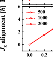
Figure 1: (Color online) The total energies (upper panels) and the alignments along the rotational axis (lower panels) as functions of the rotational frequency in ⁶⁰Fe calculated by the cranking CDFT-SLAP with separable pairing force (left panels) and monopole pairing force (right panels), respectively. The separable pairing force with $G=-728$ MeV fm³ and $a=0.644$ fm Tian et al. (2009), and the monopole pairing force with $G_{n}=G_{p}=0.8$ MeV Shi et al. (2018) are used in the particle-particle channel. For both neutron and proton, the dimensions of the MPC space are chosen as 500 (dotted lines), 1000 (dashed lines), and 2000 (solid lines), respectively. The energy at $\hbar\omega=0$ MeV calculated by separable pairing force is taken as reference.

Similar to Ref. Shi et al. (2018), by switching off pairing correlations, the validity of the cranking CDFT-SLAP with separable pairing force is checked against the TAC-CDFT calculation Zhao et al. (2011a). Here the total energies and the alignments along the rotational axis as functions of the rotational frequency in ⁶⁰Fe calculated by the cranking CDFT-SLAP, are compared with the TAC-CDFT calculations with tilted angle $\theta=0^{\circ}$ Zhao et al. (2011a). Satisfactory agreement is found with the differences less than 10^-4 MeV for the total energy and 10${}^{-4}\hbar$ for the alignment.

The convergence with respect to the major oscillator shells $N_{f}$ has been checked. By increasing $N_{f}$ from 12 to 14, the changes of the total energy and alignment for $\hbar\omega=0.2$ MeV are only 0.004$\%$ and 0.760$\%$, respectively. Thus $N_{f}=12$ are used in the present calculations.

The convergence with respect to the dimension of the MPC space has also been checked. The calculated total energies and alignments in ⁶⁰Fe by the cranking CDFT-SLAP with separable pairing force are shown in Fig. 1, compared with the results from the cranking CDFT-SLAP with monopole pairing force. For the separable pairing force, the tendency of convergence can be clearly seen. By increasing the dimensions of the MPC space from 1000 to 2000, the changes of the total energy and alignment for $\hbar\omega=0.2$ MeV are 0.151$\%$ and 0.667$\%$, respectively. In the following calculations, the dimensions of the MPC space are 1000 for both neutron and proton. For the monopole pairing force, there are no tendency of convergence with respect to the dimension of the MPC space for both the total energy and alignment. As was pointed out in Ref. Shi et al. (2018), the effective pairing strengths have to be changed when changing the dimension of the MPC space in this case.

IV Results and discussion

Three rotational bands in the nucleus ⁶⁰Fe, including the positive-parity yrast band (labeled as band A) and two negative-parity signature partner bands (labeled as bands B and C), were observed in Ref. Deacon et al. (2007). The cranking CDFT-SLAP with monopole pairing force has been applied to investigate these three bands Shi et al. (2018). In the following, the cranking CDFT-SLAP with separable pairing force will be used to calculate these three bands and compared with the data and the results in Ref. Shi et al. (2018).

IV.1 Energy spectra

In Fig. 2, the calculated total energies for the positive-parity band A and negative-parity signature partner bands B and C in ⁶⁰Fe are shown in comparison with the data Deacon et al. (2007) and the results calculated by the cranking CDFT-SLAP with monopole pairing force and without pairing from Ref. Shi et al. (2018).

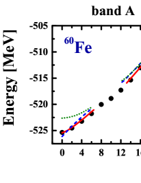
Figure 2: (Color online) The total energies for the positive-parity band A (left panel), negative-parity signature partner bands B (middle panel) and C (right panel) in ⁶⁰Fe as functions of the spin calculated by the cranking CDFT-SLAP with separable pairing force (solid lines), in comparison with the available data Deacon et al. (2007) (solid dots) and the results calculated by the cranking CDFT-SLAP with monopole pairing force (dashed lines) and without pairing (dotted lines) from Ref. Shi et al. (2018).

For band A, it is found that the cranking CDFT-SLAP with separable pairing force provides a successful description of the energy spectra, and are comparable with the cranking CDFT-SLAP with monopole pairing force. Both of them have a significant improvement on the results without pairing, in particular for the low-spin regions. There are sudden discontinuities in experimental energy sequence and intensities of the transitions at $I=8\hbar$, indicating a structural change and band crossing Deacon et al. (2007). Theoretically, all the three calculations can give this sudden change in the band structure. The band crossing obtained by the cranking CDFT-SLAP with separable pairing force occurs a bit later.

For band B, one can see that a better agreement with the data is obtained in the cranking CDFT-SLAP with separable pairing force than the cranking CDFT-SLAP with monopole pairing force, especially for the bandhead. Similar conclusion holds for band C.

IV.2 $I-\omega$ relations

In Fig. 3, the calculated angular momenta as functions of the rotational frequency are shown in comparison with the data Deacon et al. (2007), and the results calculated by the cranking CDFT-SLAP with monopole pairing force as well as without pairing from Ref. Shi et al. (2018) for bands A, B, and C.

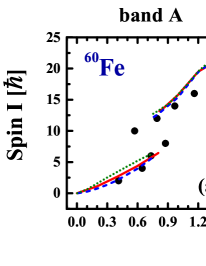
Figure 3: (Color online) The angular momenta for the positive-parity band A (left panel), negative-parity signature partner bands B (middle panel) and C (right panel) in ⁶⁰Fe as functions of the rotational frequency calculated by the cranking CDFT-SLAP with separable pairing force (solid lines), in comparison with the available data Deacon et al. (2007) (solid dots), and the results calculated by the cranking CDFT-SLAP with monopole pairing force (dashed lines) and without pairing (dotted lines) from Ref. Shi et al. (2018).

For band A, it is found that the inclusion of pairing correlations brings an improvement to the description of the $I\sim\hbar\omega$ relation, and both results given by the cranking CDFT-SLAP with separable pairing force and monopole pairing force agree well with the data. Experimentally, the $I\sim\hbar\omega$ relation shows an irregularity at spin $I=8\hbar$. As discussed in Ref. Shi et al. (2018), this corresponds to the sudden change of the configuration. The band crossing frequency obtained from the cranking CDFT-SLAP with separable pairing force is $\hbar\omega\sim 0.85$ MeV, which is a little larger than that from the cranking CDFT-SLAP calculations with monopole pairing force and without pairing ($\hbar\omega\sim 0.75$ MeV) Shi et al. (2018).

For band B, the cranking CDFT-SLAP calculations with separable pairing force and monopole pairing force give very similar results. Both of them reproduce the experimental band crossing at $\hbar\omega=1.1$ MeV well Deacon et al. (2007). For band C, similar conclusion with band B can be drawn, only that the predicted band crossing is somewhat earlier than the experimental one.

IV.3 Pairing energies

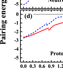
Figure 4: (Color online) The neutron and proton pairing energies for the positive-parity band A (left panel), negative-parity signature partner bands B (middle panel), and C (right panel) in ⁶⁰Fe as functions of the rotational frequency calculated by the cranking CDFT-SLAP with separable pairing force (solid lines), in comparison with the results calculated by the cranking CDFT-SLAP with monopole pairing force (dashed lines) from Ref. Shi et al. (2018).

One of the advantages of SLAP is that the pairing correlations are treated exactly and the particle number is conserved, thus there is no sharp pairing collapse in the calculations. Fig. 4 shows the neutron and proton pairing energies as functions of the rotational frequency, in comparison with the results calculated by the cranking CDFT-SLAP with monopole pairing force from Ref. Shi et al. (2018) for bands A, B, and C.

As seen in Fig. 4, both of the neutron and proton pairing energies from both the cranking CDFT-SLAP calculations with separable pairing force and monopole pairing force decrease with the rotational frequency. There is no sharp pairing collapse but rather a more continuous transition as rotational frequency is increased. However, there are evident differences in quantity between them.

For band A, before band crossing, the neutron pairing energy obtained from the cranking CDFT-SLAP with separable pairing force is smaller than that from monopole pairing force, and decreases with a smaller slope with the rotational frequency. After band crossing, the neutron pairing energy from monopole pairing force drops drastically to almost zero, while that from separable pairing force stays at around 1 MeV. The reason for this can be understood. The monopole pairing force only takes into account Cooper pairs coupled to angular momentum $J=0$. In contrast, the separable pairing force takes into account correlations not only in pairs with $J=0$, but also in pairs with higher angular momentum Tian et al. (2009).

IV.4 Shape evolutions

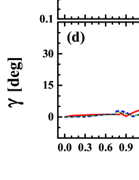
Figure 5: (Color online) The quadrupole deformation parameters $\beta$ and $\gamma$ for the positive-parity band A (left panel), negative-parity signature partner bands B (middle panel) and C (right panel) in ⁶⁰Fe as functions of the rotational frequency calculated by the cranking CDFT-SLAP with separable pairing force (solid lines), in comparison with the results calculated by the cranking CDFT-SLAP with monopole pairing force (dashed lines) and without pairing (dotted lines) from Ref. Shi et al. (2018).

In the CDFT calculation, the nuclear shape is obtained self-consistently. The shape evolutions with the rotational frequency for the three bands in ⁶⁰Fe have been investigated in Ref. Shi et al. (2018). It was found that in general the deformation parameters $\beta$ for bands A, B, and C decrease with the rotational frequency. For band A, the deformation jumps from $\beta\approx$ 0.19 to $\beta\approx$ 0.29 around the band crossing. In comparison with its signature partner band C, band B exhibits appreciable triaxial deformation Shi et al. (2018).

Figure 5 shows the evolutions of the quadrupole deformation parameters $\beta$ and $\gamma$ with the rotational frequency obtained from the cranking CDFT-SLAP with separable pairing force, in comparison with the corresponding results from monopole pairing force and without pairing. Generally speaking, the results from these three theoretical calculations are very similar. Therefore, the characteristics of the shape evolutions obtained in Ref. Shi et al. (2018) hold in the cranking CDFT-SLAP with separable pairing force calculations. It is noted that, the $\beta$ obtained from separable pairing force is slightly larger than that from monopole pairing force. This owes to two possible reasons. On the one hand, the neutron pairing energy obtained from separable pairing force is significantly smaller than that from monopole pairing force near the bandhead in band A, in corresponding with $\beta$ obtained from former calculation is about 0.02 larger than that from latter calculation during this region. On the other hand, the separable pairing force takes into account correlations in pairs with higher angular momentum, which may lead to a slightly larger $\beta$ than that from monopole pairing force in bands B, C and in the region after band crossing in band A although the pairing energy from former calculation is larger.

V Summary

In summary, a finite range separable pairing force is implemented in the shell-model-like approach based on the cranking covariant density functional theory. This method has been applied to investigate the rotational spectra observed in ⁶⁰Fe, including the positive-parity band A and negative-parity signature partner bands B and C, in comparison with the cranking CDFT-SLAP with monopole pairing force calculations. The examination of the convergence with respect to the MPC dimension shows that the calculation with separable pairing force can give better convergence than that with monopole pairing force. Excellent agreement with the available data is achieved. Furthermore, the pairing energies obtained from the cranking CDFT-SLAP with separable pairing force and monopole pairing force show evident differences in quantity that in general the pairing energy from the former calculation decreases slower with the rotational frequency than the latter one. It may be due to separable pairing force takes into account correlations not only in pairs with $J=0$, but also in pairs with higher angular momentum. This could also be the reason why the quadrupole deformation $\beta$ obtained from separable pairing force is slightly larger than that from monopole pairing force although the pairing energy from former calculation is larger.

Appendix A CALCULATION OF PAIRING MATRIX ELEMENTS

The harmonic oscillator bases one uses to solve the equation of motion (1) read

$$|n_{x}n_{y}n_{z};\alpha =+\rangle=|n_{x}n_{y}n_{z}\rangle\frac{i^{n_{y}}}{\sqrt{2}}(-1)^{n_{z}+1}\left[|\uparrow\rangle+(-1)^{n_{y}+n_{z}}|\downarrow\rangle\right],$$ (25)

$$|n_{x}n_{y}n_{z};\alpha =-\rangle=|n_{x}n_{y}n_{z}\rangle\frac{i^{n_{y}}}{\sqrt{2}}\left[|\uparrow\rangle+(-1)^{n_{y}+n_{z}+1}|\downarrow\rangle\right].$$ (26)

Here, $|n_{x}n_{y}n_{z}\rangle$ is the harmonic oscillator wave function in Cartesian coordinates, and $n_{x},~{}n_{y},~{}n_{z}$ are the corresponding quantum numbers. The labels $\alpha=+$ and $\alpha=-$ represent the states with positive and negative signature, respectively, and for simplicity they are respectively abbreviated below as $|a\rangle$ and $|\bar{b}\rangle$.

Based on these harmonic oscillator bases, the antisymmetric pairing matrix elements $\langle ab|\hat{V}_{\mathrm{pair}}|cd\rangle_{a}$ in Eq. (17) can be calculated, where the separable pairing force $\hat{V}_{\mathrm{pair}}$ (11) can be written as

$$\begin{split}\hat{V}_{\mathrm{pair}}(\bm{r}_{1},\bm{r}_{2};\bm{r}_{1}^{\prime},\bm{r}_{2}^{\prime})&=G\delta\left(\bm{R}-\bm{R}^{\prime}\right)P(\bm{r})P(\bm{r}^{\prime})\frac{1}{2}\left(1-P^{\sigma}\right)\\ &\equiv W(\bm{r}_{1},\bm{r}_{2};\bm{r}_{1}^{\prime},\bm{r}_{2}^{\prime})\frac{1}{2}(1-P^{\sigma}).\end{split}$$ (27)

There are four types of such matrix elements, i.e., $\langle a\bar{b}|\hat{V}_{\mathrm{pair}}|c\bar{d}\rangle_{a}$, $\langle ab|\hat{V}_{\mathrm{pair}}|cd\rangle_{a}$, $\langle ab|\hat{V}_{\mathrm{pair}}|\bar{c}\bar{d}\rangle_{a}$, and $\langle\bar{a}\bar{b}|\hat{V}_{\mathrm{pair}}|\bar{c}\bar{d}\rangle_{a}$. In the PAC-CDFT, the latter three types of matrix elements vanish because of the spatial symmetries fulfilled by the nuclear density distribution. As a result, only the matrix elements $\langle a\bar{b}|\hat{V}_{\mathrm{pair}}|c\bar{d}\rangle_{a}$ need to be calculated.

The antisymmetric matrix elements of the pairing interaction in Eq. (17) can be separated into a product of spin and coordinate space factors

$$\langle a\bar{b}|\hat{V}_{\rm{pair}}|c\bar{d}\rangle_{a}=\Big{\langle}a\bar{b}\Big{|}W\frac{1}{2}(1-P^{\sigma})\Big{|}c\bar{d}\Big{\rangle}_{a}.$$ (28)

The operator $\frac{1}{2}(1-P^{\sigma})$ projects onto the $S=0$ spin-singlet product state

$$\frac{1}{2}(1-P^{\sigma})|c\bar{d}\rangle=|c\bar{d}\rangle_{S=0}=\frac{1}{2}i^{n_{y}^{c}+n_{y}^{d}}(-1)^{n_{y}^{c}}\delta_{n_{y}^{c}+n_{y}^{d}+n_{z}^{c}+n_{z}^{d},\rm{even}}[|\uparrow\downarrow\rangle-|\downarrow\uparrow\rangle]|n^{c}n^{d}\rangle,$$ (29)

and the problem is reduced to the calculation of the spatial part of the matrix element

$$\begin{split}\langle a\bar{b}|\hat{V}^{\mathrm{pair}}|c\bar{d}\rangle_{a}=&\frac{1}{2}(-i)^{n_{y}^{a}+n_{y}^{b}}(-1)^{n_{y}^{a}}\delta_{n_{y}^{a}+n_{z}^{a}+n_{y}^{b}+n_{z}^{b},\mathrm{even}}\\ &\times i^{n_{y}^{c}+n_{y}^{d}}(-1)^{n_{y}^{c}}\delta_{n_{y}^{c}+n_{z}^{c}+n_{y}^{d}+n_{z}^{d},\mathrm{even}}\langle n^{a}n^{b}|W|n^{c}n^{d}\rangle.\\ \end{split}$$ (30)

The following formalisms are similar as those in Ref. Nikšić et al. (2010). The spatial part of the matrix element

$$\langle n^{a}n^{b}|W|n^{c}n^{d}\rangle\equiv 2\int\mathrm{d}\bm{r}_{1}\mathrm{d}\bm{r}_{2}\mathrm{d}\bm{r}^{\prime}_{1}\mathrm{d}\bm{r}^{\prime}_{2}~{}\phi_{n_{a}}(\bm{r}_{1})\phi_{n_{b}}(\bm{r}_{2})W(\bm{r}_{1},\bm{r}_{2};\bm{r}_{1}^{\prime},\bm{r}_{2}^{\prime})\phi_{n_{c}}(\bm{r}_{1}^{\prime})\phi_{n_{d}}(\bm{r}_{2}^{\prime}),$$ (31)

can be decomposed into three Cartesian components,

$$\langle n^{a}n^{b}|W|n^{c}n^{d}\rangle=2GW_{x}W_{y}W_{z}.$$ (32)

Here the detailed derivation of the $x$ component is given

$$W_{x}=\int\mathrm{d}x_{1}\mathrm{d}x_{2}\mathrm{d}x_{1}^{\prime}\mathrm{d}x_{2}^{\prime}~{}\phi_{n^{a}_{x}}(x_{1},b_{x})\phi_{n^{b}_{x}}(x_{2},b_{x})\delta(X-X^{\prime})P(x)P(x^{\prime})\phi_{n^{c}_{x}}(x^{\prime}_{1},b_{x})\phi_{n^{d}_{x}}(x^{\prime}_{2},b_{x}).$$ (33)

By transforming to the center-of-mass and relative coordinates, and making use of the 1D Talmi-Moshinsky transformation, the integrals over the center-of-mass coordinates $X$ and $X^{\prime}$ are solved analytically, and one can find

$$\begin{split}W_{x}=&\sum_{N_{x}}M^{n_{x}N_{x}}_{n_{x}^{a}n_{x}^{b}}I_{n_{x}}(b_{x})M^{n^{\prime}_{x}N^{\prime}_{x}}_{n_{x}^{c}n_{x}^{d}}I_{n^{\prime}_{x}}(b_{x}),\end{split}$$ (34)

where the selection rules

$$n_{x}^{a}+n_{x}^{b}=n_{x}+N_{x},~{}~{}~{}~{}~{}n_{x}^{c}+n_{x}^{d}=n^{\prime}_{x}+N^{\prime}_{x},$$ (35)

have been used to eliminate the sums over $n_{x}$ and $n^{\prime}_{x}$.

The $M^{n_{x}N_{x}}_{n_{x}^{a}n_{x}^{b}}$ denotes the 1D Talmi-Moshinsky brackets

$$\begin{split}M^{n_{x}N_{x}}_{n_{x}^{a}n_{x}^{b}}=&\sqrt{\frac{n_{x}^{a}!n_{x}^{b}!}{n_{x}!N_{x}!}}\sqrt{\frac{1}{2^{N_{x}+n_{x}}}}\delta_{n_{x}^{a}+n_{x}^{b},n_{x}+N_{x}}\sum_{m}(-1)^{n_{x}+m}\begin{pmatrix}N_{x}\\ N_{x}-n_{x}^{a}+m\end{pmatrix}\begin{pmatrix}n_{x}\\ m\end{pmatrix}.\end{split}$$ (36)

The $I_{n_{x}}(b_{x})$ reads

$$I_{n_{x}}(b_{x})=\int\mathrm{d}x~{}\phi_{n_{x}}(x,b_{x})P(x).$$ (37)

By making use of the generating function for the harmonic oscillator wave functions Nikšić et al. (2014), one can get

$$I_{n_{x}}(b_{x})=\pi^{-1/4}\sqrt{\frac{b_{x}}{b_{x}^{2}+a^{2}}}\left(\frac{a^{2}-b_{x}^{2}}{a^{2}+b_{x}^{2}}\right)^{n_{x}/2}\sqrt{\frac{n_{x}!}{2^{n_{x}}}}\frac{1}{(n_{x}/2)!}\delta_{n_{x},\mathrm{even}}.$$ (38)

To summarize, finally, the antisymmetric matrix element of the pairing interaction in Eq. (17) is

$$\langle a\bar{b}|V^{\mathrm{pair}}|c\bar{d}\rangle=G\sum_{N_{x}N_{y}N_{z}}V_{a\bar{b}}^{N_{x}N_{y}N_{z}*}V_{c\bar{d}}^{N_{x}N_{y}N_{z}},$$ (39)

which can be represented as a sum of separable terms in a 3DHO basis, with the single-particle matrix elements

$$V_{a\bar{b}}^{N_{x}N_{y}N_{z}}=i^{n_{y}^{a}+n_{y}^{b}}(-1)^{n_{y}^{a}}\delta_{n_{y}^{a}+n_{z}^{a}+n_{y}^{b}+n_{z}^{b},\mathrm{even}}V_{n^{a}_{x}n^{b}_{x}}^{N_{x}}(b_{x})V_{n^{a}_{y}n^{b}_{y}}^{N_{y}}(b_{y})V_{n^{a}_{z}n^{b}_{z}}^{N_{z}}(b_{z}).$$ (40)

The factors $V_{n^{a}_{x}n^{b}_{x}}^{N_{x}}(b_{x})$ are given by

$$V_{n^{a}_{x}n^{b}_{x}}^{N_{x}}(b_{x})=M_{n^{a}_{x}n^{b}_{x}}^{n_{x}N_{x}}I_{n_{x}}(b_{x})~{}~{}~{}\mathrm{with}~{}~{}n_{x}=n^{a}_{x}+n^{b}_{x}-N_{x}.$$ (41)

The Talmi-Moshinsky brackets $M_{n^{a}_{x}n^{b}_{x}}^{n_{x}N_{x}}$ are defined in Eq.  (36), and the integrals $I_{n_{x}}(b_{x})$ are given in Eq.  (38).

References

- Johnson et al. (1971) A. Johnson, H. Ryde, and J. Sztarkier, Phys. Lett. B 34, 605 (1971).
- Stephens and Simon (1972) F. S. Stephens and R. S. Simon, Nucl. Phys. A 183, 257 (1972).
- Twin et al. (1986) P. J. Twin, B. M. Nyakó, A. H. Nelson, J. Simpson, M. A. Bentley, H. W. Cranmer-Gordon, P. D. Forsyth, D. Howe, A. R. Mokhtar, J. D. Morrison , Phys. Rev. Lett. 57, 811 (1986).
- Frauendorf et al. (1994) S. Frauendorf, J. Meng, and J. Reif, in: M. A. Deleplanque (Ed.), Proceedings of the Conference on Physics From Large -Ray Detector Arrays, in: Report LBL35687, Univ. of California, Berkeley vol. II, p. 52 (1994).
- Frauendorf (1997) S. Frauendorf, Z. Phys. A 358, 163 (1997).
- Frauendorf (2001) S. Frauendorf, Rev. Mod. Phys. 73, 463 (2001).
- Hübel (2005) H. Hübel, Prog. Part. Nucl. Phys. 54, 1 (2005).
- Frauendorf and Meng (1997) S. Frauendorf and J. Meng, Nucl. Phys. A 617, 131 (1997).
- Meng and Zhang (2010) J. Meng and S. Q. Zhang, J. Phys. G. 37, 064025 (2010).
- Meng (2011) J. Meng, Internat. J. Modern Phys. E 20, 341 (2011).
- Meng et al. (2014) J. Meng, Q. B. Chen, and S. Q. Zhang, Internat. J. Modern Phys. E 23, 1430016 (2014).
- Meng and Zhao (2016) J. Meng and P. W. Zhao, Phys. Scr. 91, 053008 (2016).
- Xiong and Wang (2019) B. W. Xiong and Y. Y. Wang, At. Data Nucl. Data Tables 125, 193 (2019).
- Bohr and Mottelson (1975) A. Bohr and B. R. Mottelson, Nuclear tructure, vol. 2 (Benjamin, New York, 1975).
- Timár et al. (2019) J. Timár, Q. B. Chen, B. Kruzsicz, D. Sohler, I. Kuti, S. Q. Zhang, J. Meng, P. Joshi, R. Wadsworth, K. Starosta ., Phys. Rev. Lett. 122, 062501 (2019).
- Ring (1996) P. Ring, Prog. Part. Nucl. Phys. 37, 193 (1996).
- Meng et al. (2006a) J. Meng, H. Toki, S.-G. Zhou, S. Q. Zhang, W. H. Long, and L. S. Geng, Prog. Part. Nucl. Phys. 57, 470 (2006a).
- Meng and Zhou (2015) J. Meng and S.-G. Zhou, J. Phys. G 42, 093101 (2015).
- Liang et al. (2015a) H. Z. Liang, J. Meng, and S.-G. Zhou, Phys. Rep. 570, 1 (2015a).
- Meng (2016) J. Meng, ed., Relativistic Density Functional for Nuclear Structure, vol. 10 of International Review of Nuclear Physics (World Scientific, Singapore, 2016).
- Koepf and Ring (1990) W. Koepf and P. Ring, Nucl. Phys. A 511, 279 (1990).
- Peng et al. (2008) J. Peng, J. Meng, P. Ring, and S. Q. Zhang, Phys. Rev. C 78, 024313 (2008).
- Zhao et al. (2011a) P. W. Zhao, S. Q. Zhang, J. Peng, H. Z. Liang, P. Ring, and J. Meng, Phys. Lett. B 699, 181 (2011a).
- Meng et al. (2013) J. Meng, J. Peng, S. Q. Zhang, and P. W. Zhao, Front. Phys. 8, 55 (2013).
- Madokoro et al. (2000) H. Madokoro, J. Meng, M. Matsuzaki, and S. Yamaji, Phys. Rev. C 62, 061301 (2000).
- Zhao (2017) P. W. Zhao, Phys. Lett. B 773, 1 (2017).
- Yu et al. (2012) L. F. Yu, P. W. Zhao, S. Q. Zhang, P. Ring, and J. Meng, Phys. Rev. C 85, 024318 (2012).
- Zhao et al. (2011b) P. W. Zhao, J. Peng, H. Z. Liang, P. Ring, and J. Meng, Phys. Rev. Lett. 107, 122501 (2011b).
- Zhao et al. (2012) P. W. Zhao, J. Peng, H. Z. Liang, P. Ring, and J. Meng, Phys. Rev. C 85, 054310 (2012).
- Zhao et al. (2015a) P. W. Zhao, N. Itagaki, and J. Meng, Phys. Rev. Lett. 115, 022501 (2015a).
- Ren et al. (2019) Z. X. Ren, S. Q. Zhang, P. W. Zhao, N. Itagaki, J. A. Maruhn, and J. Meng, Sci. China Phys. Mech. 62, 112062 (2019).
- Meng et al. (2006b) J. Meng, J. Peng, S. Q. Zhang, and S.-G. Zhou, Phys. Rev. C 73, 037303 (2006b).
- Peng et al. (2008b) J. Peng, H. Sagawa, S. Q. Zhang, J. M. Yao, Y. Zhang, and J. Meng, Phys. Rev. C 77, 024309 (2008b).
- Yao et al. (2009) J. M. Yao, B. Qi, S. Q. Zhang, J. Peng, S. Y. Wang, and J. Meng, Phys. Rev. C 79, 067302 (2009).
- Li et al. (2011) J. Li, S. Q. Zhang, and J. Meng, Phys. Rev. C 83, 037301 (2011).
- Qi et al. (2013) B. Qi, H. Jia, N. B. Zhang, C. Liu, and S. Y. Wang, Phys. Rev. C 88, 027302 (2013).
- Ring and Schuck (1980) P. Ring and P. Schuck, The Nuclear Many-Body Problem (Springer-Verlag, Berlin, 1980).
- Zeng and Cheng (1983) J. Y. Zeng and T. S. Cheng, Nucl. Phys. A 405, 1 (1983).
- Rowe (1970) D. Rowe, Nuclear Collective Motion (Butler & Tanner Ltd, Frome and London, 1970).
- Mottelson and Valatin (1960) B. R. Mottelson and J. G. Valatin, Phys. Rev. Lett. 5, 511 (1960).
- Meng et al. (2006b) J. Meng, J. Y. Guo, L. Liu, and S. Q. Zhang, Front. Phys. China 1, 38 (2006b).
- Shi et al. (2018) Z. Shi, Z. H. Zhang, Q. B. Chen, S. Q. Zhang, and J. Meng, Phys. Rev. C 97, 034317 (2018).
- Zeng et al. (1994a) J. Y. Zeng, Y. A. Lei, T. H. Jin, and Z. J. Zhao, Phys. Rev. C 50, 746 (1994a).
- Liu et al. (2002) S. X. Liu, J. Y. Zeng, and E. G. Zhao, Phys. Rev. C 66, 024320 (2002).
- He et al. (2005) X. T. He, S. X. Liu, S. Y. Yu, J. Y. Zeng, and E. G. Zhao, Euro. Phys. J. A 23, 217 (2005).
- Wu et al. (2011) X. Wu, Z. H. Zhang, J. Y. Zeng, and Y. A. Lei, Phys. Rev. C 83, 034323 (2011).
- Zhang et al. (2013a) Z. H. Zhang, P. W. Zhao, J. Meng, J. Y. Zeng, E. G. Zhao, and S.-G. Zhou, Phys. Rev. C 87, 054314 (2013a).
- Zhang (2016a) Z. H. Zhang, Phys. Rev. C 94, 034305 (2016a).
- Liu et al. (2004) S. X. Liu, J. Y. Zeng, and L. Yu, Nucl. Phys. A 735, 77 (2004).
- Zhang et al. (2009) Z. H. Zhang, X. Wu, Y. A. Lei, and J. Y. Zeng, Nucl. Phys. A 816, 19 (2009).
- Zhang et al. (2009) Z. H. Zhang, Y. A. Lei, and J. Y. Zeng, Phys. Rev. C 80, 034313 (2009).
- Li et al. (2013) B. H. Li, Z. H. Zhang, and Y. A. Lei, Chin. Phys. C 37, 014101 (2013).
- Li and He (2016) Y. C. Li and X. T. He, Sci. China Phys. Mech. 59, 672011 (2016).
- Zhang (2016b) Z. H. Zhang, Nucl. Phys. A 949, 22 (2016b).
- Zhang et al. (2013b) Z. H. Zhang, J. Meng, E. G. Zhao, and S.-G. Zhou, Phys. Rev. C 87, 054308 (2013b).
- He et al. (2009) X. T. He, Z. Z. Ren, S. X. Liu, and E. G. Zhao, Nucl. Phys. A 817, 45 (2009).
- Zhang et al. (2011) Z. H. Zhang, J. Y. Zeng, E. G. Zhao, and S.-G. Zhou, Phys. Rev. C 83, 011304 (2011).
- Zhang et al. (2012) Z. H. Zhang, X. T. He, J. Y. Zeng, E. G. Zhao, and S.-G. Zhou, Phys. Rev. C 85, 014324 (2012).
- Liu et al. (2015) L. Liu, Z. H. Zhang, and P. W. Zhao, Phys. Rev. C 92, 044304 (2015).
- Molique and Dudek (1997) H. Molique and J. Dudek, Phys. Rev. C 56, 1795 (1997).
- Fu et al. (2013) X. M. Fu, F. R. Xu, J. C. Pei, C. F. Jiao, Y. Shi, Z. H. Zhang, and Y. A. Lei, Phys. Rev. C 87, 044319 (2013).
- Pillet et al. (2002) N. Pillet, P. Quentin, and J. Libert, Nucl. Phys. A 697, 141 (2002).
- Liang et al. (2015b) W. Y. Liang, C. F. Jiao, Q. Wu, X. M. Fu, and F. R. Xu, Phys. Rev. C 92, 064325 (2015b).
- Liu (2019) L. Liu, Phys. Rev. C 99, 024317 (2019).
- Tian et al. (2009) Y. Tian, Z. Y. Ma, and P. Ring, Phys. Lett. B 676, 44 (2009).
- Wang (2017) Y. K. Wang, Phys. Rev. C 96, 054324 (2017).
- Wang (2018) Y. K. Wang, Phys. Rev. C 97, 064321 (2018).
- Deacon et al. (2007) A. N. Deacon, S. J. Freeman, R. V. F. Janssens, M. Honma, M. P. Carpenter, P. Chowdhury, T. Lauritsen, C. J. Lister, D. Seweryniak, J. F. Smith , Phys. Rev. C 76, 054303 (2007).
- Bürvenich et al. (2002) T. Bürvenich, D. G. Madland, J. A. Maruhn, and P.-G. Reinhard, Phys. Rev. C 65, 044308 (2002).
- Nikšić et al. (2008) T. Nikšić, D. Vretenar, and P. Ring, Phys. Rev. C 78, 034318 (2008).
- Zhao et al. (2010) P. W. Zhao, Z. P. Li, J. M. Yao, and J. Meng, Phys. Rev. C 82, 054319 (2010).
- Koepf and Ring (1989) W. Koepf and P. Ring, Nucl. Phys. A 493, 61 (1989).
- König and Ring (1993) J. König and P. Ring, Phys. Rev. Lett. 71, 3079 (1993).
- Kaneko et al. (1993) K. Kaneko, M. Nakano, and M. Matsuzaki, Phys. Lett. B 317, 261 (1993).
- Koepf and Ring (1988) W. Koepf and P. Ring, Phys. Lett. B 212, 397 (1988).
- Dobaczewski and Dudek (1997) J. Dobaczewski and J. Dudek, Comput. Phys. Commun. 102, 166 (1997).
- Yao et al. (2006) J. M. Yao, H. Chen, and J. Meng, Phys. Rev. C 74, 024307 (2006).
- Nikšić et al. (2009) T. Nikšić, Z. P. Li, D. Vretenar, L. Próchniak, J. Meng, and P. Ring, Phys. Rev. C 79, 034303 (2009).
- Zeng et al. (1994b) J. Y. Zeng, T. H. Jin, and Z. J. Zhao, Phys. Rev. C 50, 1388 (1994b).
- Nikšić et al. (2010) T. Nikšić, P. Ring, D. Vretenar, Y. Tian, and Z. Y. Ma, Phys. Rev. C 81, 054318 (2010).
- Nikšić et al. (2014) T. Nikšić, N. Paar, D. Vretenar, and P. Ring, Comput. Phys. Commun. 185, 1808 (2014).