High-degree gravity modes in the single sdB star HD 4539

Abstract

HD 4539 (alias PG 0044+097 or EPIC 220641886) is a bright (V=10.2) long-period V1093 Her-type subdwarf B (sdB) pulsating star that was observed by the Kepler spacecraft in its secondary ($K2$) mission. We use the $K2$ light curve (78.7 days) to extract 169 pulsation frequencies, 124 with a robust detection. Most of these frequencies are found in the low-frequency region typical of gravity (g-)modes, but some higher frequencies corresponding to pressure (p-)modes are also detected. Therefore HD 4539 is a hybrid pulsator and both the deep and surface layers of the star can potentially be probed through asteroseismology. The lack of any frequency splitting in its amplitude spectrum suggests that HD 4539 has a rotation period longer than the $K2$ run and/or that it is seen pole-on. From asymptotic period spacing we see many high-degree modes, up to $l$=12, in the spectrum of HD 4539, with amplitudes as low as a few ppm. A large fraction of these modes can be identified and for $\sim$29% of them we obtain a unique and robust identification corresponding to $l$$\leq$8. Our study includes also a new determination of the atmospheric parameters of the star. From low-resolution spectroscopy we obtain $T_{\mathrm{eff}}$=22,800$\pm$160 K, $\log g$=5.20$\pm$0.02 and log($N$(He)/$N$(H))=–2.34$\pm$0.05. By fitting the SED we obtain $T_{\mathrm{eff}}$=23,470${}^{+650}_{-210}$ K, R_⋆=0.26$\pm$0.01 ${\mathrm{R}}_{\odot}$ and M_⋆=0.40$\pm$0.08 ${\mathrm{M}}_{\odot}$. Moreover, from 11 high-resolution spectra we see the radial velocity variations caused by the stellar pulsations, with amplitudes of $\approx$150 m/s for the main modes, and we can exclude the presence of a companion with a minimum mass higher than a few Jupiter masses for orbital periods below $\sim$300 days.

1 Introduction

Hot subdwarf stars of spectral class B (sdB) are core helium-burning stars, found both in the disk and halo of our Galaxy. Their observed properties locate them in the extreme horizontal branch (EHB) part of the H-R diagram, with effective temperatures from $\sim$22,000 to $\sim$38,000 K and surface gravities of 5.0 $\stackrel{{\scriptstyle{\displaystyle<}}}{{\sim}}$ $\log g$ $\stackrel{{\scriptstyle{\displaystyle<}}}{{\sim}}$ 6.2 in cgs units. They are compact objects with radii on the order of 0.2 $R_{\odot}$ and typical masses around 0.47 $M_{\odot}$. These stars have experienced extreme mass loss near the tip of the red giant branch, when nearly the entire hydrogen envelope was lost, leaving a helium-burning core with a very thin inert hydrogen-rich envelope ($M_{env}$ $\stackrel{{\scriptstyle{\displaystyle<}}}{{\sim}}$ 0.01 $M_{\odot}$), too thin to sustain hydrogen shell burning and ascend the asymptotic giant branch. The mechanisms responsible for this extreme mass loss are not yet well understood but it is clear that binarity plays a major role, at least for half sdB stars, those in a close binary with a white dwarf or an M-dwarf companion. The merger of two helium white dwarfs is another option to form single hot subdwarfs but only a small fraction of single sdB stars have masses large enough to be compatible with this mechanism (see e.g. discussion and Fig. 6 of Fontaine et al. 2012). Thus the formation of single sdB stars is still an open question. After depletion of helium in the core, sdB stars may evolve into subdwarf O (sdO) stars burning helium in a shell surrounding the C/O core (although a direct evolutionary link between sdB and sdO stars remains uncertain), and eventually they will end their evolutionary journey directly as a white dwarf (see Heber 2016 for a review).

About 10% of sdB stars with effective temperatures ($T_{\mathrm{eff}}$) between $\sim$28,000 and $\sim$36,000 K are found to pulsate with short period p-modes of a few minutes (Østensen et al., 2010). They are termed V361 Hya stars from the prototype (Kilkenny et al., 1997), that was discovered at about the same time at which p-modes were predicted by theory (Charpinet et al., 1996). At temperatures below 28,000 K, about 75% of sdB stars are found to be pulsating (Østensen et al., 2011) with longer-period g-modes, from $\sim$45 min up to few hours, and they are termed V1093 Her stars from the prototype (Green et al., 2003). Both p- and g-mode pulsations are driven by cyclic ionization of iron-group elements (Charpinet et al., 1997; Fontaine et al., 2003), which are pushed up by radiative levitation. Near the boundary between the two instability strips, at $T_{\mathrm{eff}}$$\approx$ 28,000 K, the so-called hybrid pulsators, that show both p- and g-modes (Baran et al., 2005; Schuh et al., 2006), offer the opportunity to probe both the external layers and the core of sdB stars.

A substantial improvement in our understanding of the stellar oscillations in sdB stars was brought by the Kepler space telescope (Borucki et al., 2010; Gilliland et al., 2010), that observed continuously 18 sdB pulsators for many months (up to more than 3 years) in its primary mission, and more than 30 pulsators for 70/90 days in its secondary mission ($K2$, Howell et al. 2014), after the second reaction wheel failed. The sampling time of 58 s of the so-called short-cadence data was not ideal for the short-period p-modes but very good for the longer-period g-modes. Thanks to the high-quality data of Kepler/$K2$, the constant period spacing predicted for the g-modes in the asymptotic limit was observed in several pulsators, as well as the missing periods due to trapped modes (Reed et al. 2011; Kern et al. 2018; Reed et al. 2018, and references therein). Multiplets of evenly spaced frequencies have confirmed that sdB stars are slow rotators, with typical periods of several days or tens of days, up to 100 days or more (Reed et al., 2018; Charpinet et al., 2018). Through period and frequency spacing it was possible to identify a large fraction of the pulsation modes detected in several stars and high-degree g-modes were seen in a few objects, up to $l$=6 (Kern et al., 2018) or $l$=8 (Telting et al., 2014a). The huge quantity of novel information contained in the Kepler/$K2$ data represents a strong challenge for seismic models and has also opened new possibilities of studying the evolution of the amplitude spectra in time, with variations of amplitudes and frequencies that are likely related to nonlinear interactions between different pulsation modes (see e.g. Zong et al. 2018). Since July 2018, the NASA $TESS$ (Transiting Exoplanet Survey Satellite) mission is continuing the work started by Kepler/$K2$ observing many new sdB pulsators and the first results are published in Charpinet et al. (2019).

In this article we describe the results of an analysis of both photometric and spectroscopic data of the sdB pulsator HD 4539 (alias PG 0044+097 or EPIC 220641886). Pulsations in this star were previously detected by Schoenaers & Lynas-Gray (2007) from line profile variations of 198 spectra acquired with the Grating Spectrograph at the 1.9 m SAAO telescope. The $K2$ light curve confirms the presence of pulsations and shows a very rich spectrum with many high-degree low-amplitude g-modes and a few p-modes, making this bright sdB star (V=10.2) one of the most interesting objects for asteroseismic studies.

2 K2 photometry

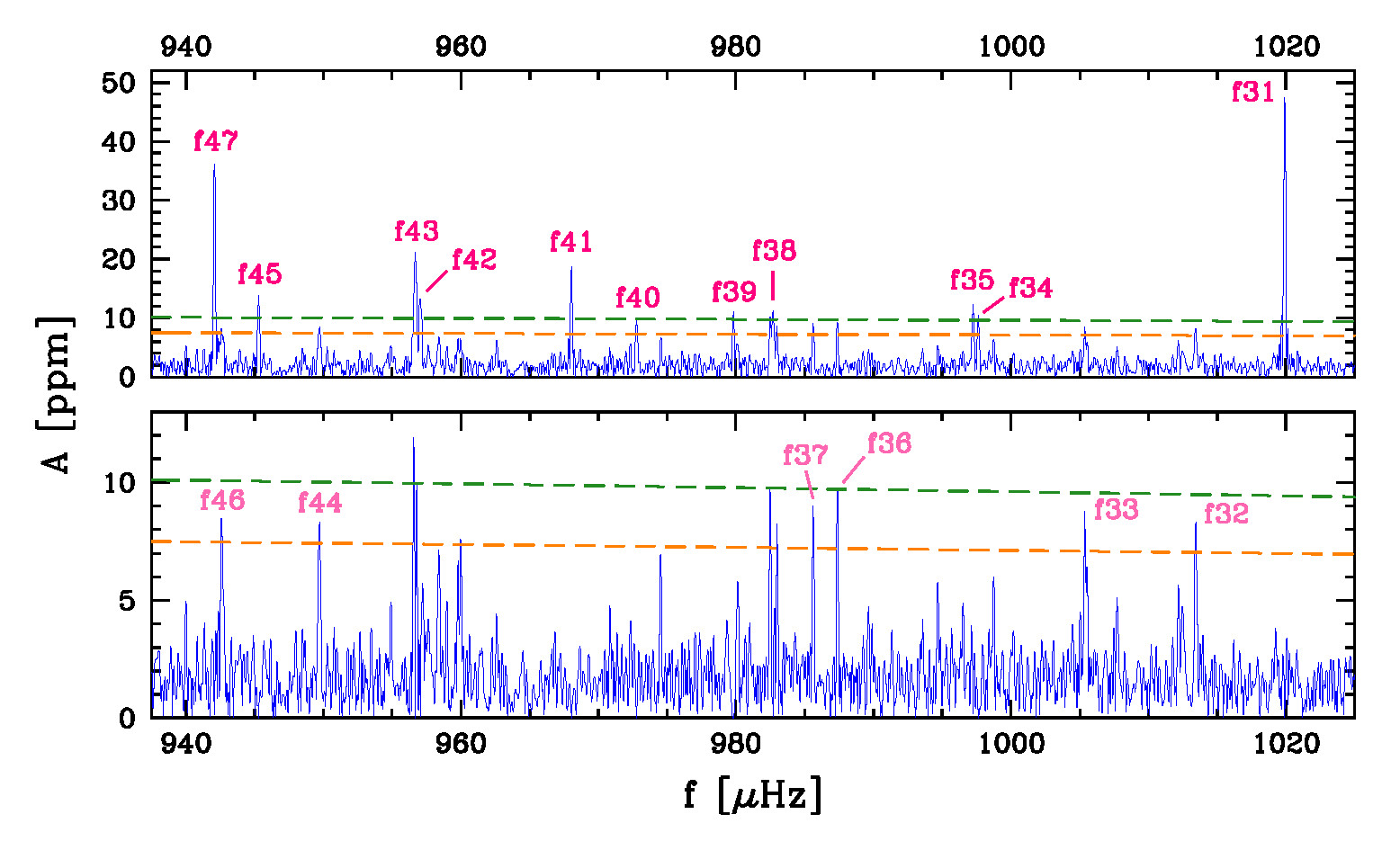
Figure 1: The 2-step procedure that we used to extract the pulsation frequencies. Top panel: the main frequencies (those with an amplitude higher than 5.4 $\sigma$, 124 in total) are extracted from the amplitude spectrum of the data. Bottom panel: once the 124 main frequencies have been subtracted from the data, secondary frequencies (45 in total, those with an amplitude between 4 and 5.4 $\sigma$) are extracted from the amplitude spectrum of the residuals. The thresholds of 4 and 5.4 $\sigma$ are represented by the orange and green lines respectively. Note that the peaks near 957 and 983 $\mu$Hz are not considered since they are just the residuals of f43 and f38, due to temporal variations of the frequencies and/or unresolved close frequencies. Instead, the peak at 960 $\mu$Hz is not considered since it was below 4 $\sigma$ in the upper panel. More details in the text.

Table 1: Pulsation frequencies.

ID	F	P	A	l	n	Notes
	[$\mu$Hz]	[s]	[ppm]
f1	4531.833	220.66	13.1	—	—
(f2	3503.332	285.44	6.2	—	—)
(f3	3499.973	285.72	5.2	—	—)
f4	3497.986	285.88	7.3	—	—	MR
(f5	3133.521	319.13	5.2	—	—)
f6	2969.824	336.72	8.6	—	—
f7	2969.661	336.74	7.6	—	—
f8	2968.864	336.83	9.8	—	—
f9	2968.701	336.85	7.3	—	—
f10	2968.444	336.88	12.4	—	—
(f11	2963.608	337.43	5.3	—	—)
f12	2945.414	339.51	7.5	—	—
(f13	2941.457	339.97	6.0	—	—)
(f14	2516.795	397.33	4.9	—	—)
f15	2329.916	429.20	9.4	—	—	MR
——  approximate boundary between p- and g-modes  ——
(f16	1704.969	586.52	6.3	—	—)
(f17	1683.290	594.07	5.5	—	—)
f18	1465.086	682.55	7.7	—	—
f19	1397.473	715.58	10.4	—	—
f20	1246.915	801.98	9.0	—	—
f21	1227.676	814.55	8.3	—	—
f22	1227.170	814.88	9.5	—	—
(f23	1226.799	815.13	6.0	—	—)
f24	1166.801	857.04	7.6	—	—	MR
(f25	1105.843	904.29	6.2	10	28)	TI
(f26	1077.765	927.85	6.6	9	26)	or l=12, n=35
(f27	1067.695	936.60	7.0	—	—)
f28	1067.503	936.77	9.7	10	29	TI
f29	1034.893	966.28	22.8	9	27	TI; NoR
f30	1025.764	974.88	11.6	—	—
f31	1019.899	980.49	48.4	12	37	TI; NoR
(f32	1013.432	986.75	8.5	—	—)
(f33	1005.356	994.67	8.7	7	22)	or l=8, n=24
f34	997.620	1002.39	9.7	9	28	or l=10, n=31
f35	997.230	1002.78	12.5	10	31	or l=9, n=28
(f36	987.372	1012.79	9.6	—	—)
(f37	985.603	1014.61	9.1	—	—)
f38	982.680	1017.63	11.0	6	19	TI; MR
f39	979.808	1020.61	10.1	—	—
f40	972.769	1027.99	9.5	—	—
f41	968.027	1033.03	18.5	12	39	TI; NoR
f42	957.031	1044.90	16.5	—	—
f43	956.670	1045.29	24.0	—	—	MR
(f44	949.703	1052.96	8.4	—	—)
f45	945.282	1057.89	13.7	—	—
(f46	942.577	1060.92	8.8	—	—)
f47	942.061	1061.50	36.7	12	40	TI
f48	919.003	1088.14	34.8	12	41	or l=7, n=24; SR
f49	912.554	1095.83	12.6	—	—
f50	904.752	1105.28	39.3	10	34	TI; NoR
(f51	902.985	1107.44	9.4	—	—)
(f52	896.904	1114.95	8.4	9	31)	or l=12, n=42
f53	896.305	1115.69	14.5	12	42	or l=9, n=31
f54	894.152	1118.38	11.8	—	—
(f55	890.156	1123.40	9.5	8	27)	TI
f56	885.065	1129.86	20.7	6	21	TI MR
f57	881.686	1134.19	26.6	7	25	TI
f58	879.016	1137.64	11.0	10	35	TI
f59	877.037	1140.20	12.8	12	43	TI
f60	867.057	1153.33	11.7	9	32	TI
f61	864.231	1157.10	36.8	—	—	MR

Table 2: continued

ID	F	P	A	l	n	Notes
	[$\mu$Hz]	[s]	[ppm]
(f62	857.000	1166.86	9.5	8	28)	TI
f63	855.757	1168.56	11.1	12	44	or l=10, n=36
f64	853.968	1171.00	21.2	10	36	or l=12, n=44
f65	841.157	1188.84	18.5	9	33	TI
(f66	836.247	1195.82	9.6	—	—)
f67	835.861	1196.37	11.0	—	—
f68	835.416	1197.01	24.4	12	45	TI
f69	828.161	1207.49	13.4	8	29	or l=10, n=37
(f70	823.361	1214.53	8.7	—	—)
f71	818.056	1222.41	33.8	12	46	or l=9, n=34; or l=7, n=27
(f72	808.031	1237.58	8.8	10	38)	or l=6, n=23
(f73	798.261	1252.72	8.8	8	30)	or l=12, n=47, SR
f74	793.296	1260.56	14.5	9	35	TI
f75	785.720	1272.72	19.6	7	28	TI
(f76	771.070	1296.90	8.0	—	—)
f77	770.607	1297.68	10.7	9	36	TI, SR
(f78	770.277	1298.23	8.4	—	—)
f79	757.778	1319.65	19.5	7	29	TI
f80	756.461	1321.95	10.7	—	—
(f81	752.619	1328.69	8.3	—	—)
f82	741.650	1348.34	24.2	6	25	TI
f83	734.678	1361.14	19.1	12	51	TI
f84	732.627	1364.95	28.8	—	—
f85	732.476	1365.23	52.4	7	30	TI
(f86	707.210	1414.01	8.6	12	53)	or l=7, n=31
(f87	702.790	1422.90	8.8	8	34)	TI
(f88	700.061	1428.45	8.8	—	—)
f89	682.352	1465.52	13.3	8	35	TI
f90	681.253	1467.88	11.6	12	55	TI
f91	679.234	1472.25	10.8	10	45	TI
f92	645.689	1548.73	19.4	8	37	or l=12, n=58; PLC1
(f93	634.943	1574.95	9.0	12	59)	or l=6, n=29
(f94	625.742	1598.10	7.3	7	35)	TI
f95	622.754	1605.77	14.0	10	49	or l=12, n=60
f96	613.476	1630.05	13.1	9	45	or l=12, n=61 or l=6, n=30
f97	611.943	1634.14	26.4	8	39
(f98	604.148	1655.22	10.2	12	62)	TI
f99	593.813	1684.03	16.4	6	31	or l=12, n=63
f100	593.579	1684.70	28.1	12	63	or l=6, n=31; MR
f101	581.916	1718.46	20.6	8	41
f102	567.798	1761.19	17.4	8	42
f103	557.560	1793.53	58.1	6	33	SR
f104	541.799	1845.70	12.8	8	44
f105	540.767	1849.23	31.4	12	69	TI; MR
f106	540.551	1849.97	45.7	6	34
f107	525.061	1904.54	72.5	6	35
f108	524.847	1905.32	39.0	10	58	TI
f109	510.027	1960.68	164.4	6	36	SR
(f110	503.468	1986.22	11.5	5	31)
(f111	495.961	2016.29	8.1	6	37)
f112	487.276	2052.22	36.0	5	32	MR
(f113	482.714	2071.62	9.5	6	38)
f114	472.533	2116.25	35.5	5	33	MR
f115	470.009	2127.62	42.1	6	39	MR
f116	458.005	2183.38	33.6	5	34	or l=6, n=40; or l=4, n=28
f117	446.757	2238.35	69.3	6	41	MR
f118	445.031	2247.03	23.0	5	35	MR
f119	441.287	2266.10	38.6	4	29	NoR
f120	432.204	2313.72	26.2	5	36	MR
f121	409.048	2444.70	52.0	5	38	MR
f122	399.031	2506.07	41.8	4	32	MR
f123	386.847	2585.00	41.3	4	33	MR

Table 3: continued

ID	F	P	A	l	n	Notes
	[$\mu$Hz]	[s]	[ppm]
f124	384.362	2601.71	77.3	—	—	SR
f125	374.989	2666.74	20.3	4	34	NoR
f126	353.644	2827.71	61.6	4	36	MR; PLC2
f127	343.924	2907.62	18.9	4	37
f128	325.591	3071.34	52.6	4	39	or l=6, n=56; NR
(f129	309.680	3229.14	12.6	4	41)	or l=5, n=50
f130	272.740	3666.50	185.5	2	25	NoR
f131	262.856	3804.37	47.0	2	26
f132	234.551	4263.47	217.1	2	29	NoR
f133	226.883	4407.56	83.4	—	—	PLC3
f134	226.772	4409.72	79.5	2	30
(f135	212.630	4703.01	21.6	2	32)
(f136	200.065	4998.36	26.3	2	34)	or l=1, n=20
f137	199.019	5024.65	103.8	1	20	or l=2, n=34; NR
f138	184.250	5427.40	52.0	—	—	PLC4
f139	183.842	5439.44	69.5	2	37	MR
(f140	178.849	5591.29	30.8	2	38)	PLC5
(f141	174.249	5738.90	28.8	2	39)	PLC6
f142	165.701	6034.97	74.8	2	41
(f143	145.725	6862.25	42.8	1	27)
f144	144.346	6927.78	49.1	2	47
f145	140.381	7123.45	68.7	1	28
f146	135.588	7375.29	180.0	2	50	or l=1, n=29
f147	126.811	7885.73	55.7	1	31
f148	125.496	7968.39	163.3	2	54
f149	123.141	8120.80	75.9	2	55	or l=1, n=32
f150	119.146	8393.06	355.3	1	33	or l=2, n=57; MR
f151	115.962	8623.53	131.4	1	34
f152	115.645	8647.18	62.5	—	—
f153	112.324	8902.79	223.3	1	35	MR
f154	106.398	9398.65	150.4	1	37	SR
f155	102.991	9709.61	73.2	1	38	TI
f156	102.856	9722.33	70.1	2	66	TI
f157	100.875	9913.29	502.5	1	39	SR
f158	95.776	10440.98	457.4	1	41	MR
(f159	92.884	10766.12	50.9	2	73)
f160	91.298	10953.08	322.4	1	43	SR
f161	89.230	11207.02	146.6	1	44
f162	85.032	11760.31	81.3	1	46	TI
f163	83.396	11990.97	796.1	1	47	NoR
f164	80.035	12494.57	231.9	1	49
f165	78.508	12737.50	321.9	1	50	or l=2, n=86; MR
f166	77.842	12846.60	144.5	2	87
f167	73.613	13584.56	74.9	2	92	or l=1, n=53
f168	68.027	14700.08	71.5	2	99	or l=1, n=58
f169	65.073	15367.46	306.0	2	104	or l=1, n=60
The overtone n in column 6 is arbitrarily defined assuming that $n$=1
corresponds to the first positive pulsation period starting from zero
(and assuming a constant period spacing down to $n$=1).
Notes: TI=Tentative Identification.
SR=Strong Residuals after prewhitening due to amplitude/
frequency variations and/or unresolved close frequencies.
MR=Moderate Residuals after prewhitening due to potential
ampl./freq. variations and/or unresolved close frequencies.
NoR=No Residuals after prewhitening: single stable peak.
PLC1=Potential Linear Combination: |f92-(f109+f146)|=0.074$\mu$Hz.
PLC2: |f126-(f132+f150)|=0.053$\mu$Hz.
PLC3: |f133-(f146+f160)|=0.003$\mu$Hz.
PLC4: |f138-(f150+f169)|=0.031$\mu$Hz, |f138-(f154+f166)|=0.010$\mu$Hz,
|f138-(f157+f163)|=0.021$\mu$Hz.
PLC5: |f140-(f157+f166)|=0.132$\mu$Hz.
PLC6: |f141-(f158+f165)|=0.035$\mu$Hz.

2.1 Pulsation frequencies

HD 4539 was observed for 78.7 days by $K2$ in short cadence from BJD_TBD 2457392.058531 to 2457470.781242 (corresponding to 04/01/2016 – 23/03/2016). We downloaded all available data from the “Barbara A. Mikulski Archive for Space Telescopes” (MAST). We used the short-cadence (SC) data, sampled at 58.85 s time resolution, since they allow us to reasonably sample an amplitude spectrum beyond the g-mode region, which means that both g-and p-mode regions are covered.

First, we used standard IRAF tasks to extract fluxes from the pixel tables. Next, we used our custom Python scripts to decorrelate fluxes in X and Y directions. This latter step removed the flux dependence on position on the CCD and the resultant light curve was free of the signatures of thruster firings. Finally, the light variations were converted to residual flux ($f/\bar{f}-1$) in parts per million (ppm).

In order to extract the pulsation frequencies from the light curve we used the following procedure: first we defined the mean noise level of the amplitude spectrum. This was done by selecting 123 peaks higher than a certain treshold in the amplitude spectrum of the data, regardless of whether they were true pulsation frequencies or not, subtracting these frequencies from the light curve (pre-whitening), computing the amplitude spectrum of the residuals, and applying to it a cubic spline interpolation. This cubic spline interpolation represents the mean noise level ($\sigma$) as a function of frequency. At this point we started the real extraction of the pulsation frequencies assuming a 5.4 $\sigma$ threshold, which corresponds to a 95% confidence level for $K2$ data following Baran et al. (2015). A low-frequency peak at 37.3 $\mu$Hz was excluded a-priori because the corresponding period of $\sim$26,800 s is too close to 6-7 hours, which is the typical time between two re-pointings of the $K2$ telescope (see e.g. Fig. 1 of Vandenburg & Johnson 2014).
The frequency extraction was done in two steps:
1) we selected from the amplitude spectrum of the data 83 high-amplitude peaks ($>$7.0 $\sigma$). Secondary peaks very close to the main peaks were excluded in this phase. The frequencies, amplitudes and phases of these 83 main signals were optimized using a least-square fit with 83$\times$3=249 free parameters. This is about the maximum number of parameters for which we obtain a robust convergence of the least-square solution. From here on the least-square optimization of further frequencies was done one by one, optimizing frequency, amplitude and phase of each new entry but keeping fixed the frequencies of the 83 main peaks (but not their amplitudes and phases). 30 further frequencies were added, with lower amplitudes but still higher than 5.4 $\sigma$. Furthermore, we added also 11 “close frequencies” bringing the total number of robust detections to 124 (see Table 1). As “close frequencies” we mean those frequencies that are close to one of the previous 113 (83+30) peaks, but distant enough to be resolved at half of their maximum amplitude (half maximum). Frequencies not resolved at half maximum are not considered in Table 1. Again, frequencies, amplitudes and phases of the close frequencies were optimized keeping fixed the frequencies of the 113 previous peaks (but not their amplitudes and phases).
2) From the amplitude spectrum of the residuals (light curve – 124 frequencies) we selected 45 further peaks with an amplitude higher than 4.0 $\sigma$, which corresponds to about 50% confidence level (Baran et al., 2015), and we verified that their amplitude was higher than 4.0 $\sigma$ also in the amplitude spectrum of the data. These 45 low-amplitude frequencies are considered only as candidates and are shown in brackets in Table 1. An example of our 2-step procedure to extract the pulsation frequencies is shown in Fig. 1.

2.2 Frequency multiplets, inclination, stellar rotation

In the amplitude spectrum of HD 4539 we do not see any signature of multiplets of equally spaced frequencies, suggesting a very long rotation period, longer than the $K2$ light curve, or a very low inclination of the rotation axis with respect to the line of sight or both. The rotation velocity of HD 4539 was measured by Geier & Heber (2012), who obtained v_rot sin$i$=3.9$\pm$1.0 km/s, using 21 absorption lines from FEROS spectra. If we assume a stellar radius of 0.26$\pm$0.01 ${\mathrm{R}}_{\odot}$ (see section 3), this measurement translates into P_rot/sin$i$=3.4$\pm^{1.3}_{0.8}$ days, corresponding to a rotational frequency splitting of $\sim$1.7/sin$i$ $\mu$Hz ($l$=1) or 2.8/sin$i$ $\mu$Hz ($l$=2). With a high inclination these frequency splittings would be easily seen given the $\sim$0.15 $\mu$Hz frequency resolution of the $K2$ data. With a low inclination the frequency splittings would be even larger but the amplitude of the $m$$\neq$0 modes would be lower. However, given the high quality of the $K2$ data, some of the low-amplitude components of the multiplets should be visible, e.g. the $m$=$\pm$1 components of the $l$=2 modes (Pesnell, 1985). Therefore, if we want to reconcile the absence of frequency splittings with the spectroscopic result of Geier & Heber (2012), the only possibility would be an extremely low inclination and a very short rotation period of the order of hours. But very short rotation periods are unusual in sdB pulsators and seem to happen only in close binaries (Reed et al., 2018; Charpinet et al., 2018). Given that HD 4539 does not have close companions (see section 4), we conclude that the rotation velocity of 3.9/sin$i$ km/s should be considered just as an upper limit. This interpretation is also supported by the fact that pulsational line broadening is certainly present in this star. The RV variations of several hundred meters per second that we measured (section 4) include both vertical and horizontal motions. But we know that the horizontal velocity field is dominant in g-modes so that the horizontal velocities, whose contribution is maximum at the limb of the star, just as the rotation does, may easily reach several km/s. In conclusion: 1) we do not have reasons to believe that the rotation period is much different from the relatively long periods found in almost all the other sdB pulsators. 2) This star must have a very long rotation period and/or a very low inclination. This is further confirmed by the fact that some of the main peaks in the amplitude spectrum (those indicated with “NoR” in the last column of Table 1) are completely removed when subtracting a single sine wave, indicating that there are no unresolved multiplets in these cases.

2.3 Period spacing

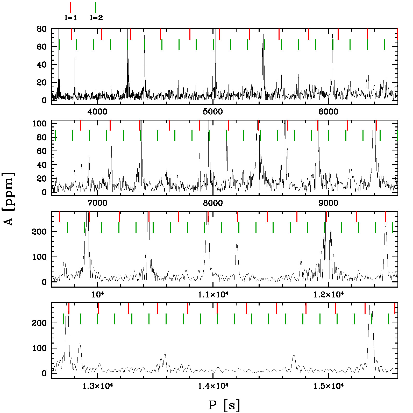
Figure 2: Period spacing for the modes with $l$=1,2: both sequences are well defined.

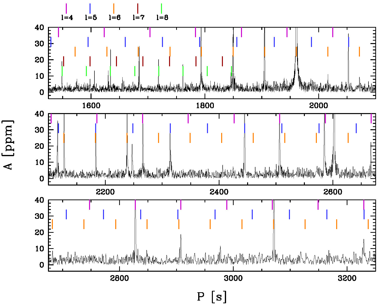
Figure 3: Period spacing for the modes with 4$\leq$$l$$\leq$8. Note the clean sequence of modes with $l$=4 (between $\sim$2260 and $\sim$3230 s), $l$=5 ($\sim$2050–2450 s, with 5 consecutive modes), $l$=6 ($\sim$1680–2240 s, with at least 9 consecutive modes) and $l$=8 ($\sim$1550–1850 s). The modes with $l$=7 are not active in this region and can be seen at shorter periods in Fig. 4.

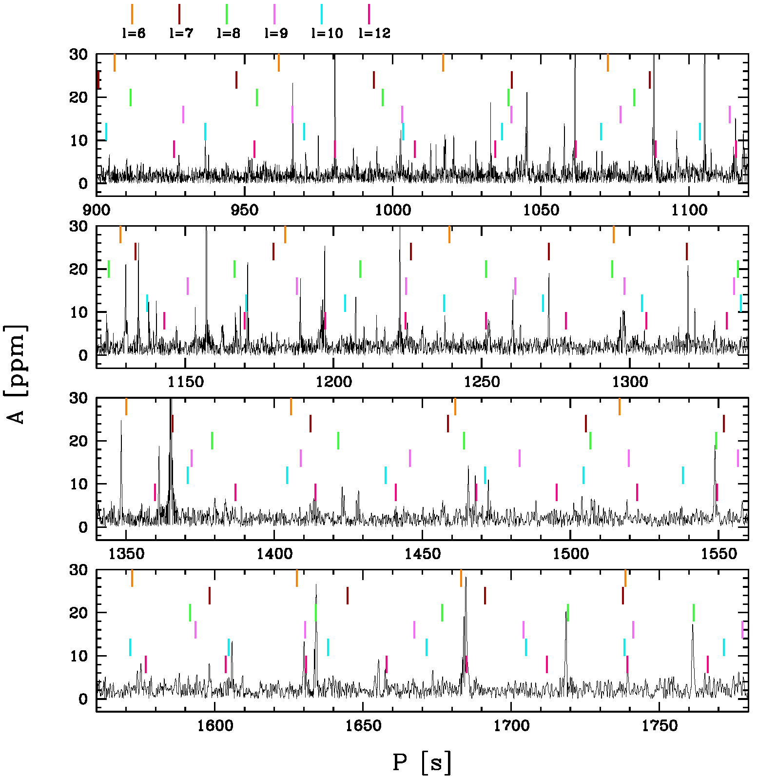
Figure 4: Period spacing for the modes with 6$\leq$$l$$\leq$12. The high concentration of peaks at short periods implies that modes with high degree, up to at least $l$=12, must be present in this star. However it makes the mode identification very difficult. Sequences with at least 2 or 3 consecutive peaks can be recognized for $l$=7 ($\sim$1090–1370 s) and $l$=8($\sim$1550–1760 s, see also Fig. 3), and partially also for $l$=9 ($\sim$1190–1300 s), $l$=10 ($\sim$905–1240 s), and $l$=12 ($\sim$980 to at least 1200).

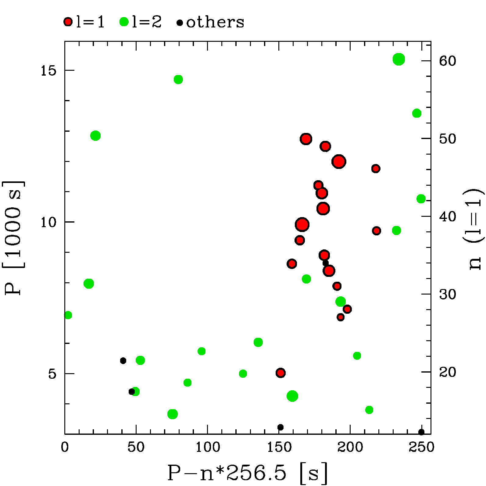
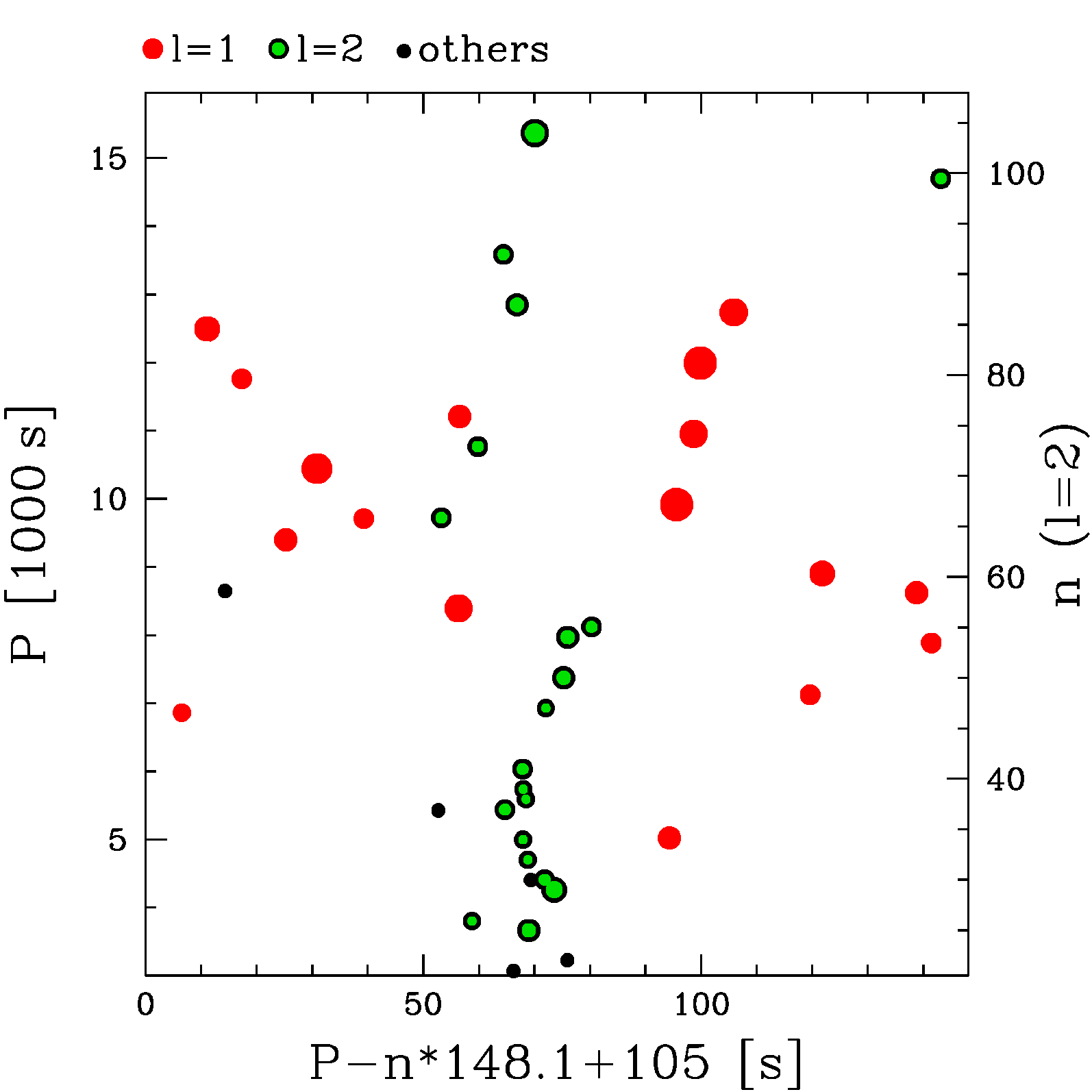
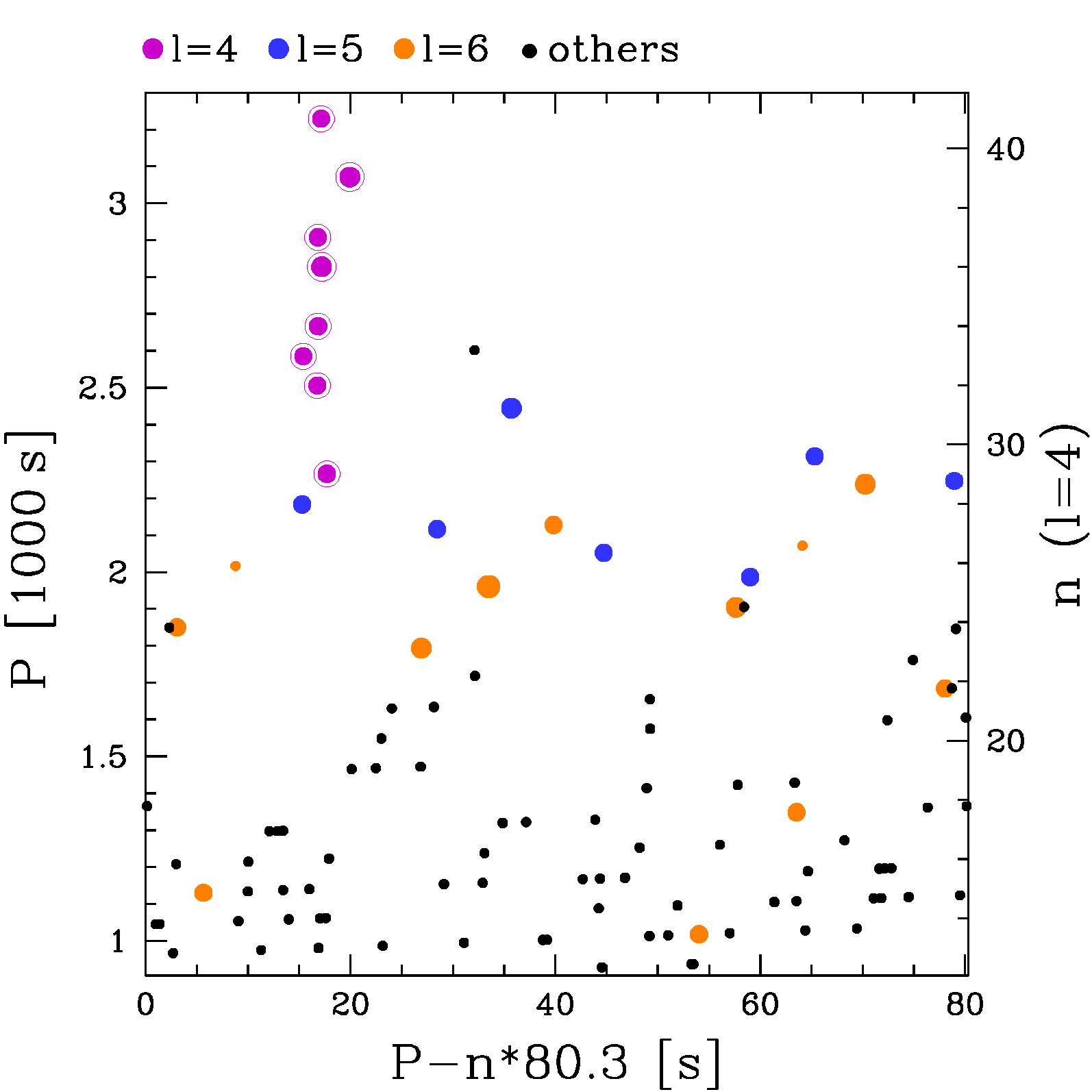
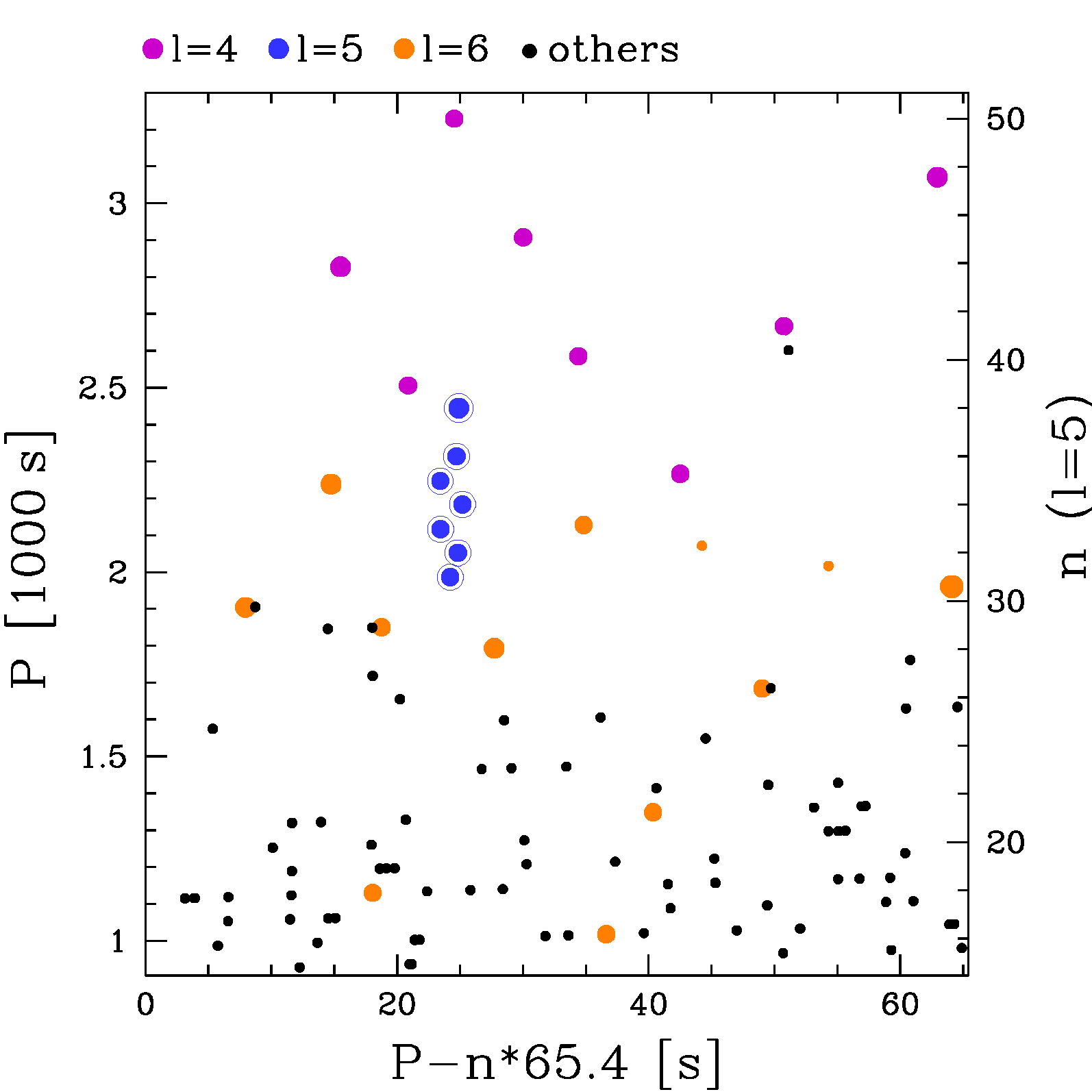
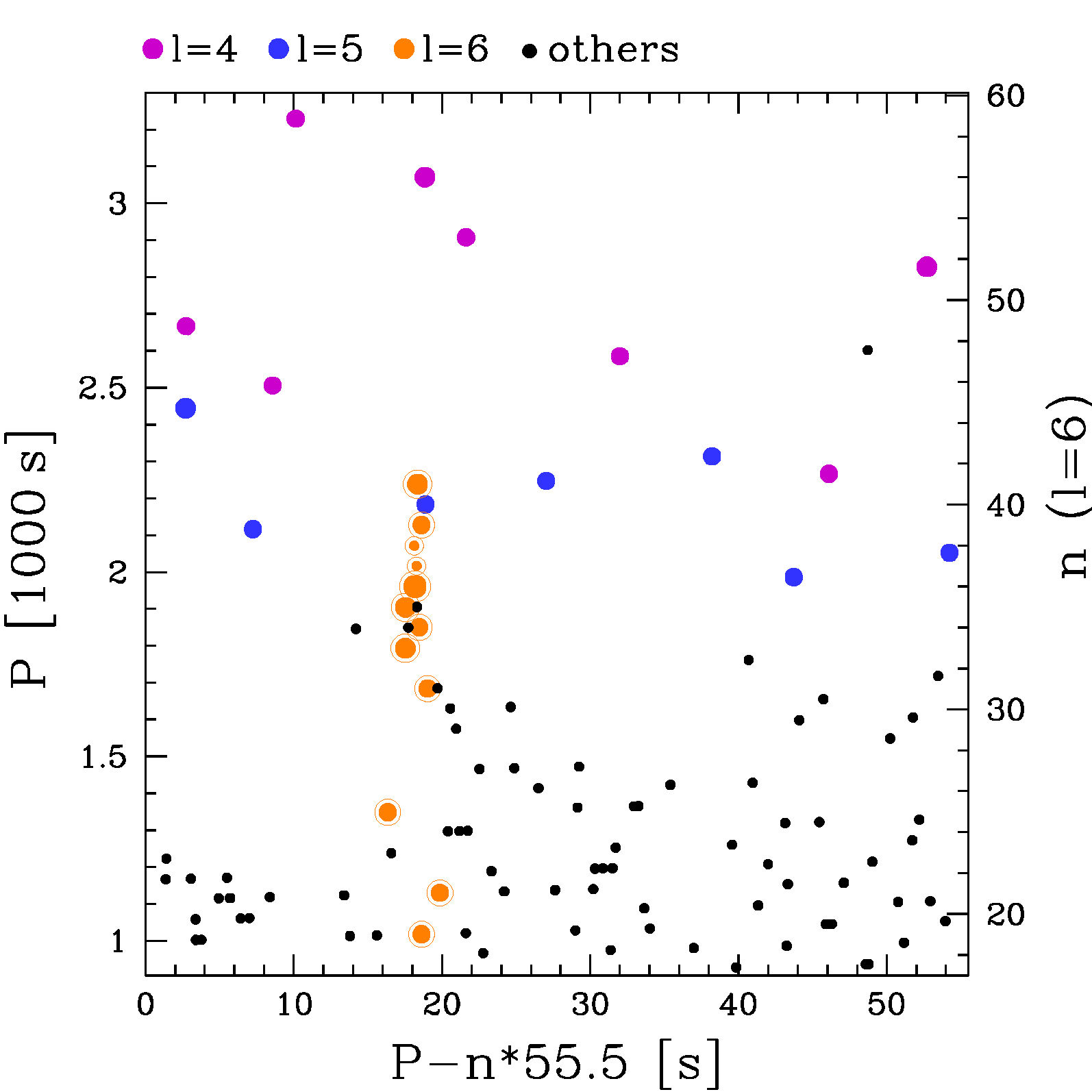
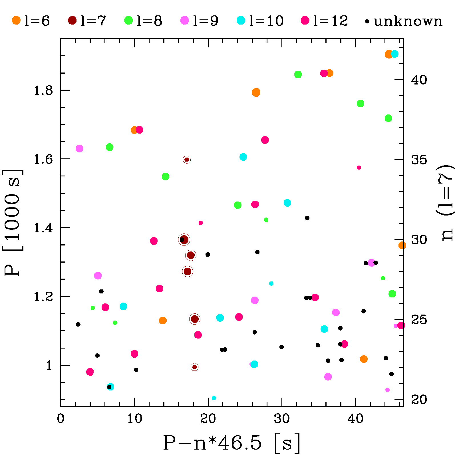
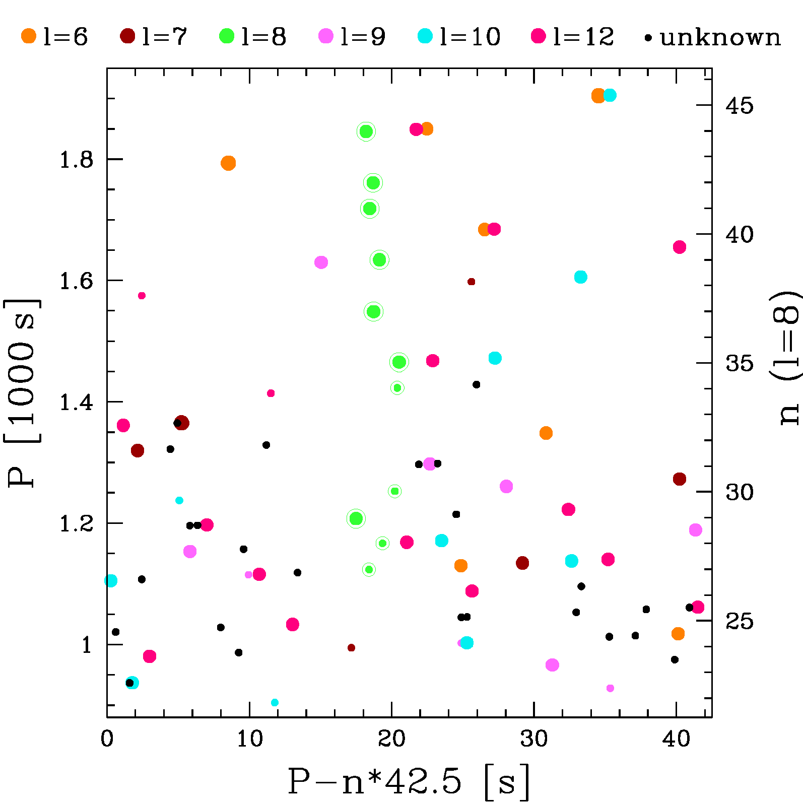
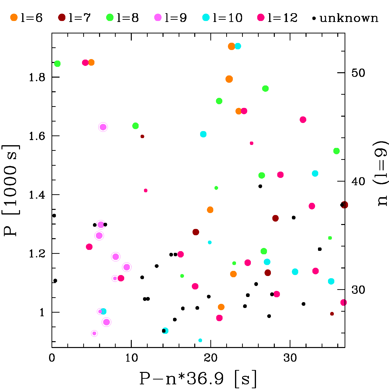
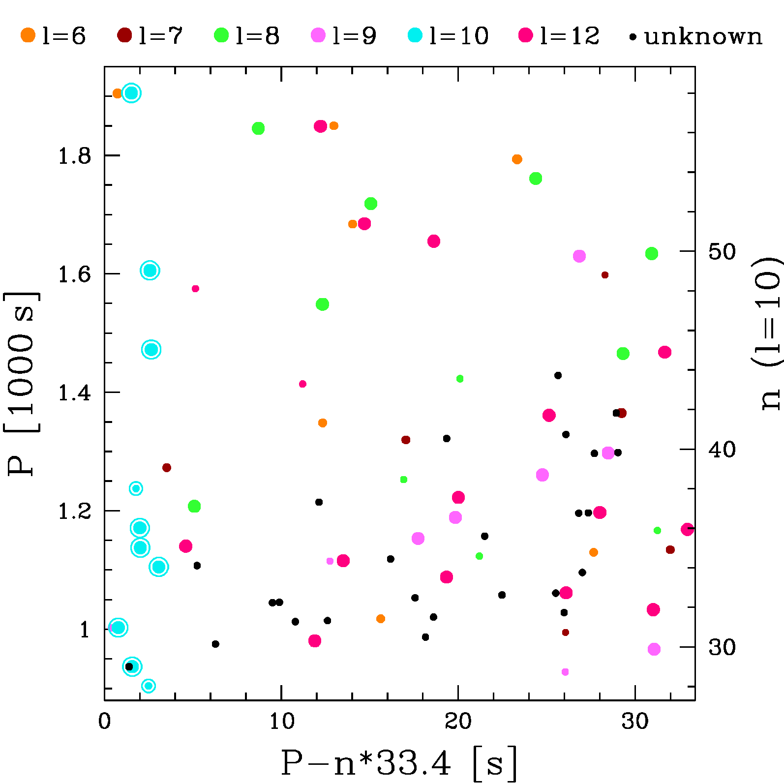
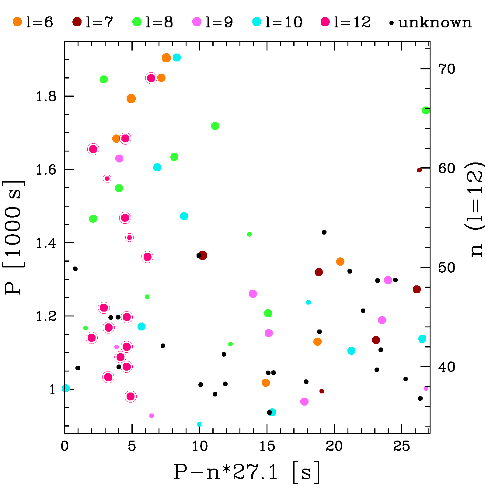
Figure 5: Echelle diagrams of the modes with $l$=1,2,4,5,6,7,8,9,10,12. The size of each point is proportional to the amplitude of that mode. An offset of 105 s was applied to the upper right panel ($l$=2) just for clarity.

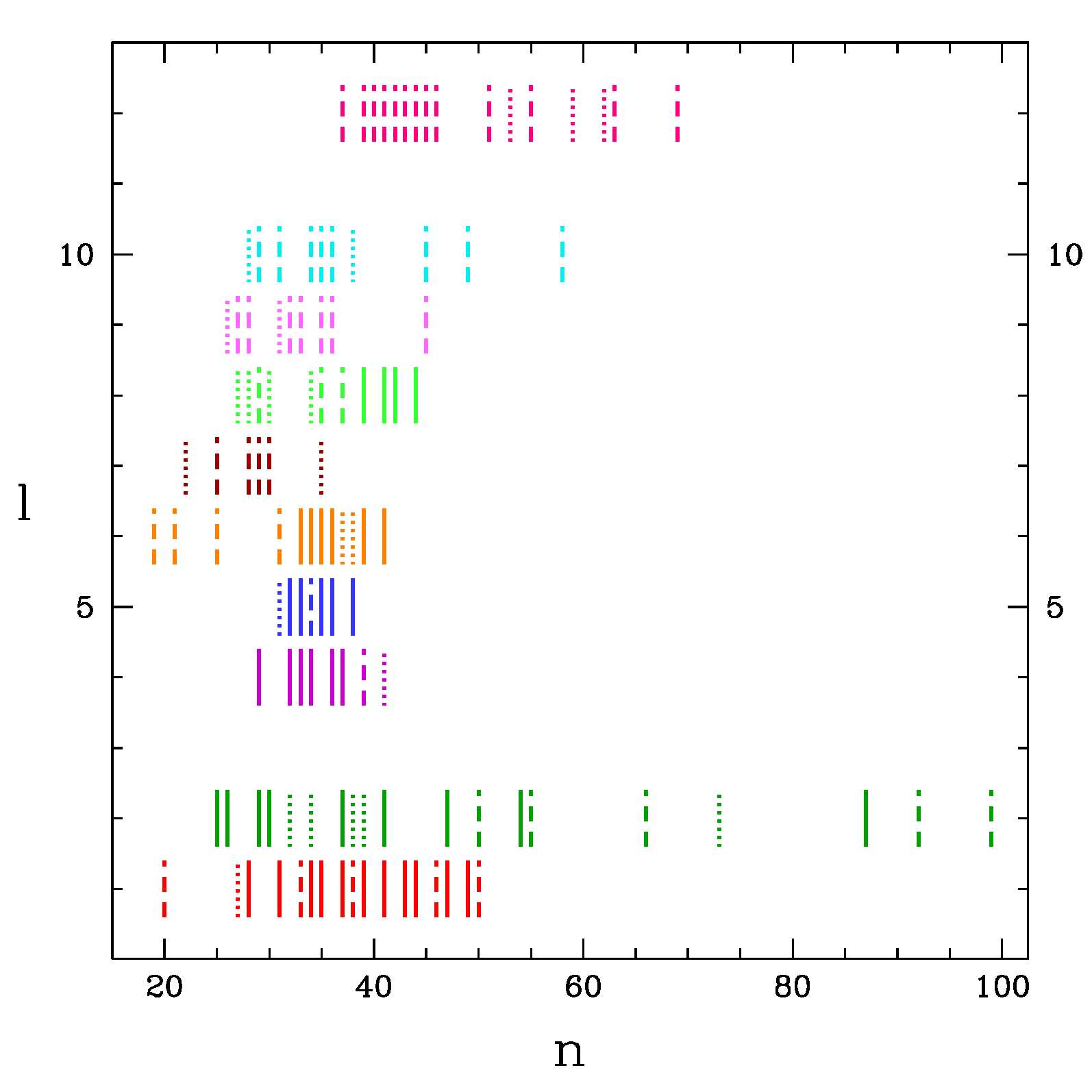
Figure 6: Summary of all identified g-modes. Dotted segments correspond to the modes with only 50% confidence level (reported in brackets in Table 1), dashed segments correspond to the modes with a tentative identification.

When we plot the amplitude spectrum as a function of the pulsation period (Fig. 2, 3 and 4), we clearly see sequences of modes that are evenly spaced in period. This corresponds to what is expected from theory in the asymptotic approximation ($n$$\gg$$l$) for high-order g-modes: $\Delta$$P_{l}$=$\Delta$$\Pi$/$[l(l+1)]^{1/2}$, where $\Delta\Pi$ is the reduced period spacing, which is typically close to 350 s for these stars. In practice we can derive $\Delta$$\Pi$ by measuring $\Delta$$P_{1}$ or $\Delta$$P_{2}$ and then compute the expected $\Delta$$P_{l}$ for $l$$>$2. From Fig. 2 we see that the two sequences with $l$=1 and $l$=2 are well defined, at least up to $\sim$12,500 s. Longer-period modes, up to $\sim$15,400 s, are present but their identification is less certain and it is not clear if these modes are $l$=1 or $l$=2. In both $l$=1 and $l$=2 sequences we do not see any clear signature of mode trapping in the high-order (long-period) region. Looking at the échelle diagrams in Fig. 5 (upper plots), only 3 modes appear to be shifted with respect to their normal position ($l$=1, $n$=38,46 and $l$=2, $n$=99) but their identification is not certain. As shown by Charpinet et al. (2014), the lack of trapped modes in the high-order region does not automatically mean that the star has a less stratified structure with respect to classical chemically stratified sdB models. Lower-order $l$=1 or $l$=2 modes, with periods below 3,600 s, where mode trapping could be more active, do not seem to be excited in this star. The average period spacing that we obtain for $l$=1 and $l$=2, 256.5 s and 148.1 s, correspond to a basically identical reduced period spacing of 362.75 and 362.77 s respectively, from which we can compute the expected period spacing for the modes with higher degree. In Fig. 3 the sequences with $l$=4, $l$=5, $l$=6 and $l$=8 are easily recognizable. The $l$=7 sequence is visible at shorter periods in Fig. 4. The $l$=3 sequence is not seen. Considering that Kepler’s response function extends from 4200 to 9000 Å with a maximum near 6000 Å, the fact that we do not see $l$=3 modes in our data is compatible with the expectation that these modes have much lower amplitudes in the optical at increasing wavelength (Randall et al., 2005). However the same article predicts particularly high amplitudes in the red for the $l$=5 modes, which we do not see. In Fig. 4 we see a large number of low-amplitude peaks at ever shorter periods, making difficult the mode identification in this region. The density of modes implies that modes with high degree, up to at least $l$=12, are present in this star: we see sequences of at least 2 or 3 consecutive peaks with $l$=7 and $l$=8 and partially also $l$=9, $l$=10 and $l$=12, while apparently we do not see consecutive $l$=11 modes. More details are given in the caption of Fig. 4. In Fig. 5 the échelle diagrams of the sequences with $l$=1,2,4,5,6,7,8,9,10,12 are shown. In Fig. 6 a summary of all the identified g-modes is given. We note that for most degrees the excited modes have about the same range of overtone index $n$. This kind of properties can be useful for comparison with models in future studies. See for example Fig. 9, 11 and 12 of Jeffery & Saio 2006, (although these authors consider only $l$=1,2,3,4 modes), or Fig. 6 of Bloemen et al. (2014) from which, potentially, we might obtain also some indication on the evolutionary status of the star (although the stars considered in that article are much hotter than HD 4539).

2.4 Linear combinations

In order to verify if some of the low-amplitude modes listed in Table 1 correspond to linear combinations of the main modes (those with an amplitude higher than 100 ppm), we computed f1+f2 and 2f1 for all the main modes. When the difference (in absolute value) between a mode frequency and the linear combination is less than 0.15 $\mu$Hz (the formal frequency resolution), a flag is given in column 7 of Table 1. In particular, a linear combination may explain why we could not find an identification for f133 and f138, the latter corresponding to three different combinations.

2.5 Frequency and amplitude time variations

From the continuous light curves produced by $Kepler$ and $K2$ we have learned that oscillation frequencies in sdB stars are not as stable as previously believed (see e.g. Reed et al. 2014) and, at least in one case, they may even show a stochastic behavior (Østensen et al., 2014). A systematic study of these aspects is presented by Zong et al. (2018). Even though the much longer $Kepler$ light curves are more suitable to study these aspects, a short analysis of the frequency/amplitude variations of HD 4539 was performed using sliding Fourier Transforms (sliding FTs) to see how the pulsation frequencies and amplitudes vary over the course of the 78.7 days of observation. We divided the $K2$ light curve into 30 subsets of about 20.7 days each, moving forward the beginning of each subset of two days at each step, and we computed the amplitude spectrum of each subset. From Table 1 we selected a few high-amplitude frequencies which are particularly variable (those marked with "SR=Strong Residuals after prewhitening" in the last column of Table 1) or, on the contrary, particularly stable (marked with “NoR=No Residuals” in the last column of Table 1). The sliding FTs of these frequencies are shown in Fig. 7.

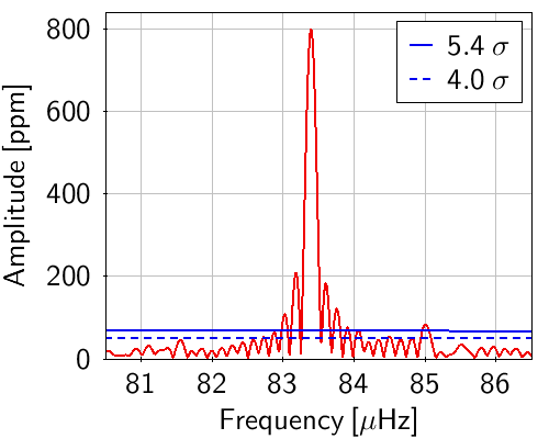
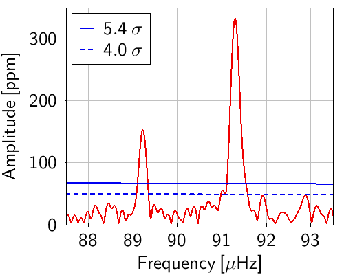
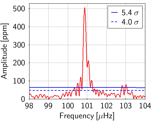
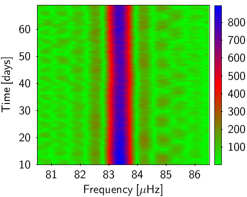
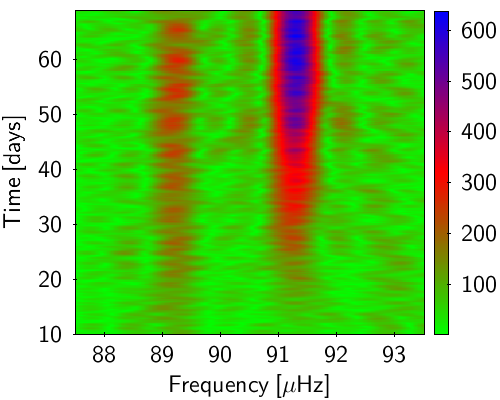
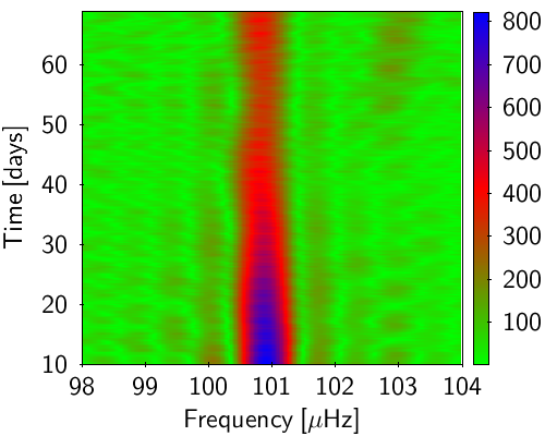
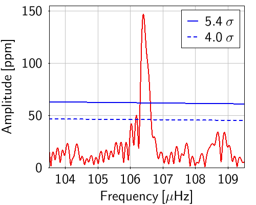
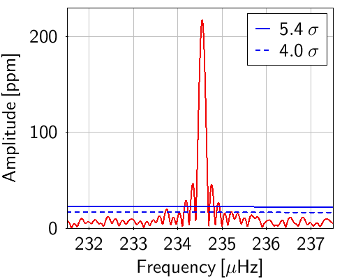
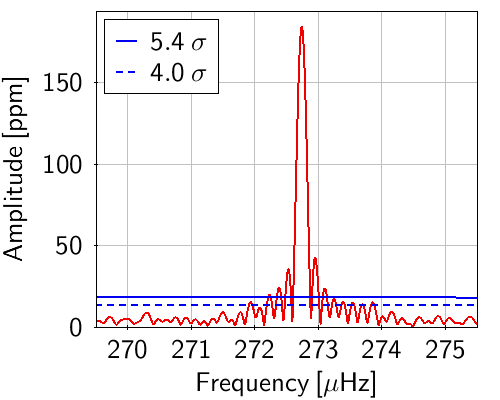
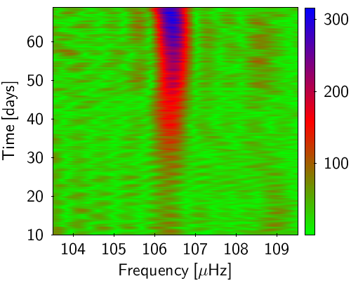
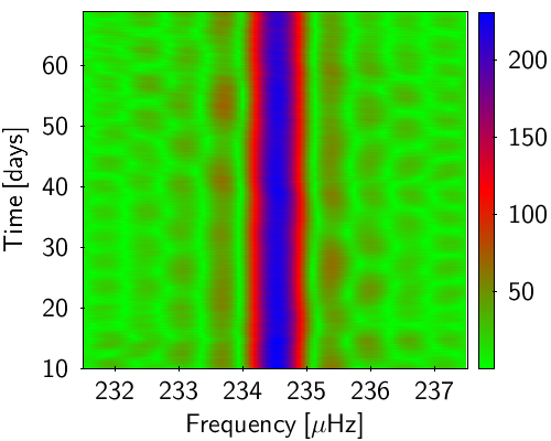
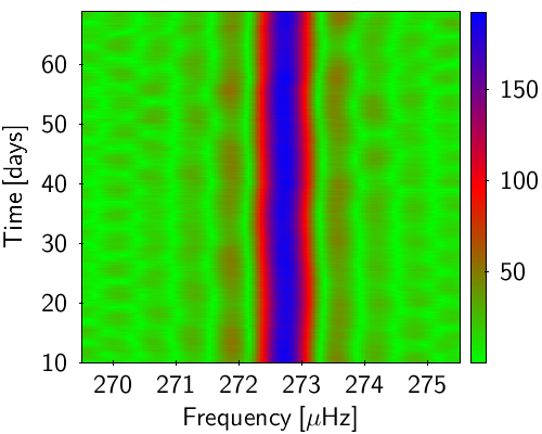
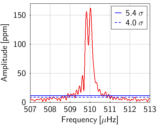
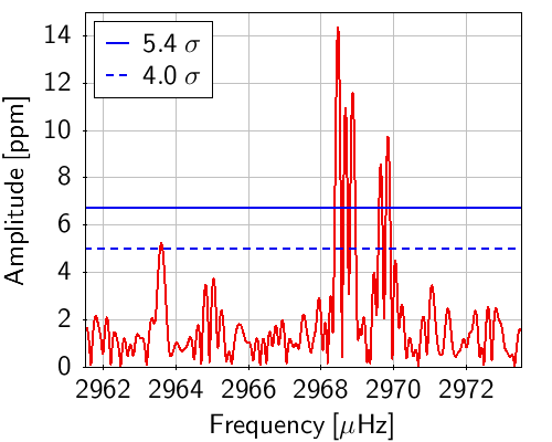
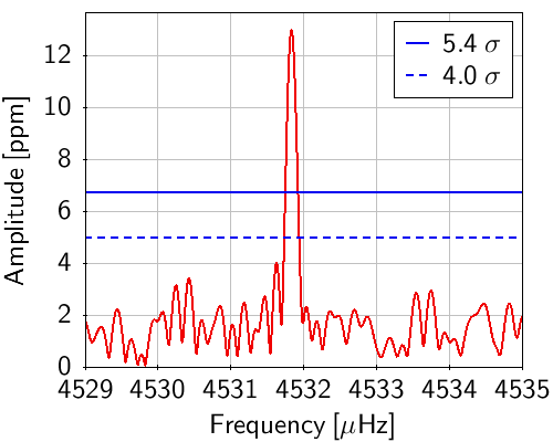
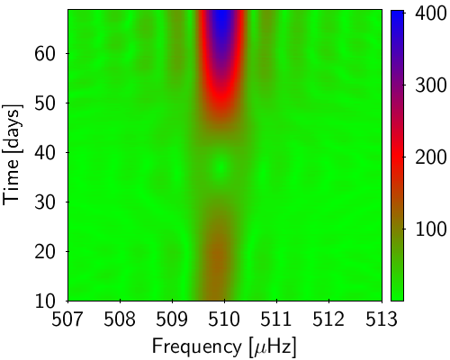
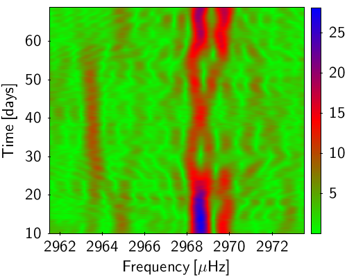
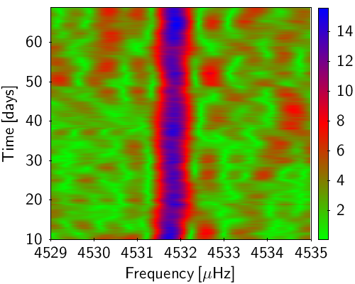
Figure 7: Sliding FTs of some of the main pulsation modes. From from top left to bottom right f163, f160, f157 and f154 ($l$=1); f132 and f130 ($l$=2); f109 ($l$=6); f6-f11 and f1 (p-modes). We see that some modes, like f130, f132 and partially f163 are stable both in frequency and amplitude, while others show variations that are particularly strong in amplitude. The color coded amplitude is given in ppm.

3 Low-resolution spectroscopy, SED, and atmospheric parameters

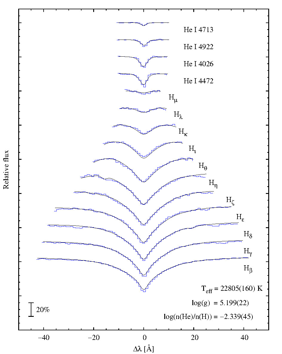
Figure 8: Atmospheric parameters of HD 4539 as obtained from the sum of 3 ALFOSC spectra.

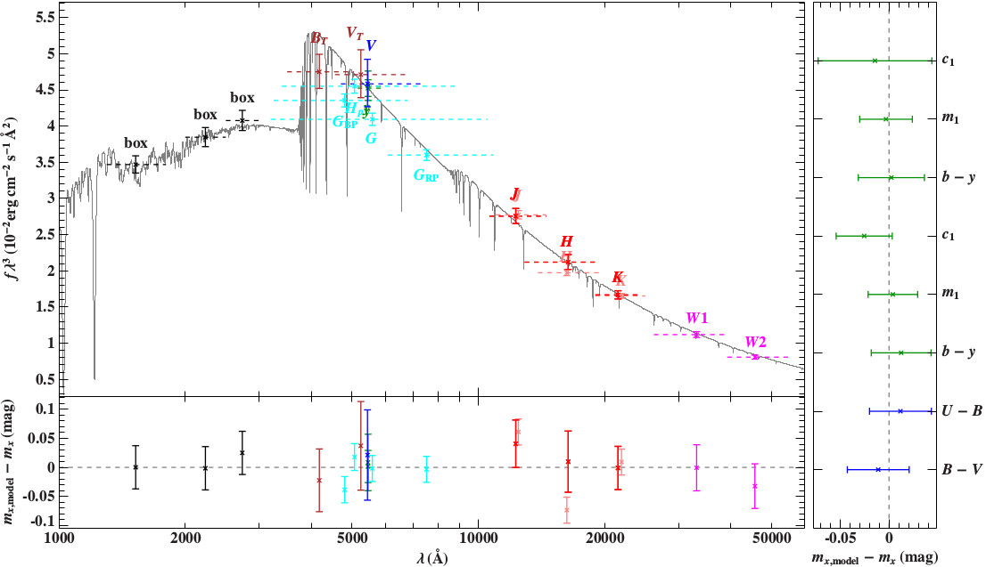
Figure 9: Spectral energy distribution of HD 4539. Colored data points represent the filter-averaged fluxes, which were converted from observed magnitudes (the filter widths are indicated by dashed horizontal lines), while the gray solid line represents a synthetic spectrum computed from a model atmosphere. The 3 box “filters” in the UV band, which cover the range 1300-1800, 2000-2500, and 2500–3000 Å, are extracted from IUE spectra (see Heber et al. 2018 for more details). The bottom/right panels show the differences between synthetic and observed magnitudes/colors. The following color codes are used to identify the photometric systems: UV (black), Tycho (brown), Johnson (blue), Hypparcos/Gaia (cyan), Strömgren (green), 2MASS (red), and WISE (magenta).

Given its brightness and long history in sdB literature, there are several determinations of the atmospheric parameters of HD 4539, sometimes with significant differences: $T_{\mathrm{eff}}$=25,000$\pm$2000 K, $\log g$=5.4$\pm$0.2 (Baschek, Sargent & Searle, 1972); $T_{\mathrm{eff}}$=24,800 K, $\log g$=5.4, log($N$(He)/$N$(H))=–2.32$\pm$0.05 (Heber & Langhans, 1986); $T_{\mathrm{eff}}$$\simeq$27,000 K, $\log g$$\simeq$5.46, log($N$(He)/$N$(H))=–2.30 (Saffer et al., 1994); $T_{\mathrm{eff}}$=25,200 K, $\log g$=5.40 (Cenarro et al., 2007); $T_{\mathrm{eff}}$=26,000$\pm$500 K, $\log g$=5.2$\pm$0.1, log($N$(He)/$N$(H))=–2.32$\pm$0.05 (Sale, Schoenaers & Lynas-Gray, 2008); $T_{\mathrm{eff}}$=23,000 K (Geier & Heber, 2012); $T_{\mathrm{eff}}$=23,200$\pm$100 K, $\log g$=5.20$\pm$0.01, log($N$(He)/$N$(H))=–2.27$\pm$0.24 (Schneider et al., 2018).

As part of our K2 sdBV follow-up spectroscopic survey (Telting et al., 2014b), we did a new determination of the atmospheric parameters of HD 4539 using three low-resolution spectra (R$\sim$2000, or 2.2 Å) taken at the 2.56 m Nordic Optical Telescope (NOT, La Palma) with ALFOSC, grism#18, 0.5 arcsec slit, and CCD#14, giving an approximate wavelength range 345-535 nm. The observations were carried out on the night starting on 2016-12-07. The spectra were homogeneously reduced and analysed. Standard reduction steps within IRAF include bias subtraction, removal of pixel-to-pixel sensitivity variations, optimal spectral extraction, and wavelength calibration based on helium arc-lamp spectra. The peak signal-to-noise ratio of the individual spectra is in excess of 200. By fitting 11 Balmer lines and 4 He I lines (Fig. 8) we obtain $T_{\mathrm{eff}}$=22,800$\pm$160 K, $\log g$=5.20$\pm$0.02 and log($N$(He)/$N$(H))=–2.34$\pm$0.05, in good agreement with Schneider et al. (2018). The values that we obtain are relative to the H/He LTE grid of Heber et al. (2000). The errors are the formal fitting errors, which only reflect the S/N of the mean spectrum and the match to the model, and not any systematic effects caused by the assumptions underlying those models, which can be an order of magnitude larger.

An independent determination of $T_{\mathrm{eff}}$ was derived also by fitting, with an appropriate model atmosphere, the spectral energy distribution (SED) obtained from available photometric measurements covering all wavelenghts from the ultraviolet to the infrared (Fig. 9), following the method described by Heber et al. 2018 (see also Schindewolf et al. 2018). Here we just mention the sources of the photometric data. We used ultraviolet fluxes extracted from IUE spectra (downloaded from the “Mikulski Archive for Space Telescopes” (MAST)), Tycho $B_{T}$, $V_{T}$ magnitudes and Hypparcos $H_{P}$ magnitude (ESA, 1997), Gaia DR2 magnitudes ($G$, $G_{BP}$, $G_{RP}$, see Gaia Collaboration et al. 2018), 2MASS J, H, K (Skrutskie et al. 2006) and WISE W1, W2 (Cutri et al., 2013) infrared magnitudes. Johnson V magnitude and colors and Strömgren colors from VizieR (Ochsenbein, Bauer & Marcout, 2000) were also included. Adopting $\log g$=5.20$\pm$0.05, we obtain $T_{\mathrm{eff}}$=23,470${}^{+650}_{-210}$ K, an angular diameter $\Theta$=$\left(6.38^{+0.06}_{-0.10}\right)$$\times$10^-11 rad and zero interstellar reddening (E(B–V)$<$0.009). If we combine the angular diameter with the Gaia DR2 parallax $\varpi$=5.384$\pm$0.132 mas (or d=185.7${}^{+4.7}_{-4.4}$ pc), we obtain for HD 4539 a radius of 0.263${}^{+0.009}_{-0.011}$ ${\mathrm{R}}_{\odot}$ and a mass of 0.40$\pm$0.08 ${\mathrm{M}}_{\odot}$ from the relation M=$g$ $\Theta^{2}$d²/(4 G).

4 High-resolution spectroscopy and radial velocities

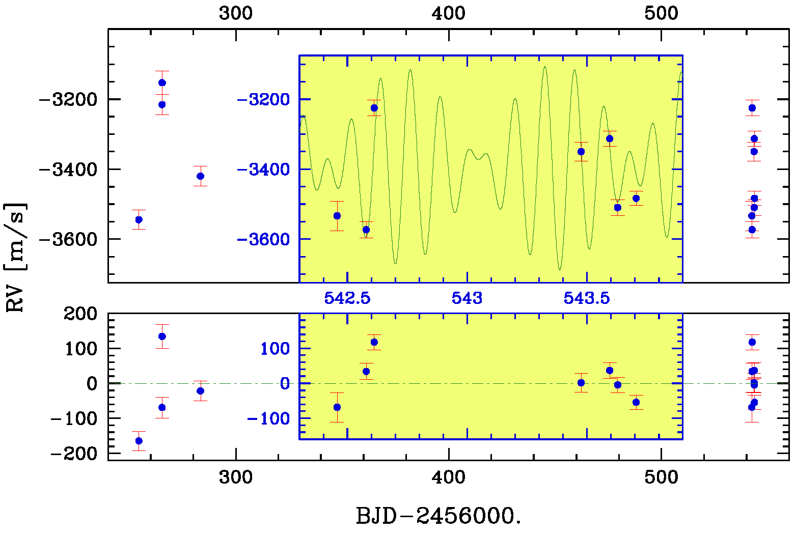
Figure 10: Upper panel: radial velocities of HD 4539 and best sinusoidal fit using the 3 highest-amplitude pulsation frequencies from Table 1 (f163, f157 and f158). Lower panel: residuals. The 2 yellow insets show a magnification of the 2nd run.

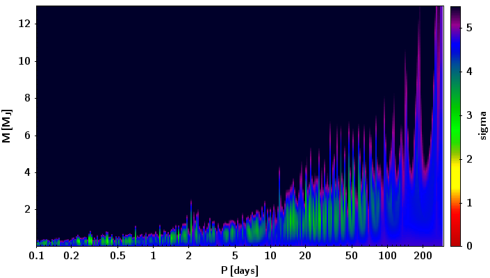
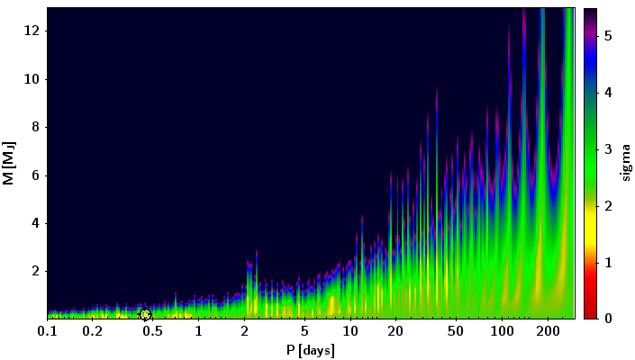
Figure 11: Upper limits to the mass of a hypothetical companion to HD 4539 as a function of orbital period. The upper panel is obtained using the RV data (upper panel of Fig. 10) while in the lower panel we used the RV residuals (lower panel of Fig. 10). The regions where the presence of a companion would be best compatible with the RV measurements are those in yellow/green. The counterintuitive fact that the “good” regions are smaller in the upper panel highlights the difficulty of fitting the RV data with a single orbital frequency when the RV variations are caused by several pulsation frequencies. In the lower panel a viewfinder at P$\simeq$0.45 d and M sin$i$$\simeq$0.15 $\rm M_{\rm Jup}$ shows the best point in terms of minimum difference between RV residual and synthetic RV value. See text for more details.

HD 4539 was observed with Harps-N at the Telescopio Nazionale Galileo (TNG, La Palma) in 2 runs (November-December 2012 and September 2013) and we collected in total 11 high-resolution spectra with a mean signal-to-noise ratio of 102. While a chemical abundance analysis is beyond the scope of this article, here we concentrate on the radial velocity (RV) measurements. Using the cross correlation function on more than 200 absorption lines (excluding H and He lines that are too broad), we computed the RVs of the star and we found a system velocity of –3392.7 m/s with significant variations around this value that are attributed to the g-mode pulsations (Fig. 10). With only 11 points it is obviously not possible to determine the RV amplitude of each pulsation mode. However, by fitting these 11 RVs with the three highest-amplitude pulsation frequencies from Table 1, we can at least obtain a zero-order measurement of the RV amplitudes involved. Assuming constant frequencies, we obtain amplitudes of 146, 164 and 40 m/s for f163, f157 and f158 respectively.

The residuals shown in the lower panel of Fig. 10 can be used to obtain an upper limit to the minimum mass (M sin$i$) of a hypothetical companion. We computed a series of synthetic RV curves for different orbital periods and companion masses and compared these curves with the RV residuals. For each synthetic RV curve we selected the best phase using a weighted least squares algorithm. For each observational point we computed the difference, in absolute value and in $\sigma$ units (where $\sigma$ is the observation error), between RV residual and synthetic RV value. The color coding in Fig. 11 corresponds to the mean value of this difference. We should keep in mind, however, that these upper limits to the mass of a companion are likely overestimated given that the residuals shown in the lower panel of Fig. 10 still contain some residual signal due to the many pulsation modes that were not considered in our fit.

5 Summary

The analysis of the $K2$ data on HD 4539 shows a very rich spectrum, with several g-modes of high-degree, up to at least $l$=12. To our knowledge, this is the first time that $l$=12 modes are seen in an sdB star and that sequences of consecutive modes with $l\geq$4, up to at least $l$=8, are clearly recognized. G-modes with such high degree are very rare also in other types of pulsating stars except, perhaps, $\delta$ Scuti stars (see e.g. Dziembowski et al. 1998; Mantegazza et al. 2012). The identification of these high-degree g-modes in HD 4539 is made possible by the absence of rotational splitting of the frequencies, which makes the spectrum cleaner, and by the star brightness, which makes it possible to detect amplitudes below 10 ppm. Therefore this star represents a challenge and an ideal laboratory to test current asteroseismic models. Thanks to the simultaneous presence of a few p-modes as well, potentially both the internal layers near the core and the external layers of the star can be probed through seismic tools. We have not been able to identify any trapped modes in the sequences of HD 4539, but such identifications are extremely hard when the mode sequences are incomplete and the order of individual modes cannot be verified with rotational splittings.

The absence of multiplets points towards a rotation period longer than the $K2$ light curve and/or a very low inclination. This is further strengthened by the presence of a few high-amplitude peaks in the Fourier spectrum that are completely removed when subtracting a single sinusoidal wave, suggesting that there are no unresolved multiplets in these cases. When we consider the rotation velocity obtained by Geier & Heber (2012), if the line broadening they measured was actually due only to rotation it would imply an extremely low inclination and a fast rotation with a period of the order of hours, which appears unlikely, also considering that part of the line broadening is produced by the pulsations.

Our new determination of the atmospheric parameters of HD 4539 confirms that this star is close to the low-temperature boundary of the g-mode instability strip, where the p-modes are normally not present. We know only one other sdB pulsator, KIC 2697388 (alias SDSS J190907.14+375614.2), showing both g- and p-modes at $T_{\mathrm{eff}}$ below $\sim$24,000 K (Kern et al., 2017). The reason why only these 2 relatively cool stars show p-modes is not clear. In the case of HD 4539 its brightness is certainly helpful in detecting ppm-level modes, but to answer this question we probably need larger statistics and the $TESS$ mission can help in this respect.

The RV measurements obtained from high-resolution spectroscopy show significant variations due to the pulsations, with amplitudes of the order of 150 m/s for the main modes, and allow us to exclude the presence of a companion with a minimum mass higher than a few Jupiter masses for orbital periods below $\sim$300 days.

Appendix A Some extra material

References

- Baran et al. (2005) Baran A., Pigulski A., Kozieł D., Ogłoza W., Silvotti R., Zoła S., 2005, MNRAS, 360, 737
- Baran et al. (2015) Baran A., Koen C., Pokrzywka B., 2015, MNRAS, 448, L16
- Baschek, Sargent & Searle (1972) Baschek B., Sargent W. L. W, Searle L., 1972, ApJ, 173, 611
- Bloemen et al. (2014) Bloemen S. et al., 2014, A&A, 569, A123
- Borucki et al. (2010) Borucki W. J. et al., 2010, Science, 327, 977
- Cenarro et al. (2007) Cenarro A. J. et al., 2007, MNRAS, 374, 664
- Charpinet et al. (1996) Charpinet S., Fontaine G., Brassard P., Dorman B., 1996, ApJ, 471, L103
- Charpinet et al. (1997) Charpinet S., Fontaine G., Brassard P., Chayer P., 1997, ApJ, 483, L123
- Charpinet et al. (2014) Charpinet S., Brassard P., Van Grootel V., Fontaine G., 2014, ASPC, 481, 179
- Cutri et al. (2013) Cutri R. M. et al., 2013, VizieR Online Data Catalog, 2328
- Charpinet et al. (2018) Charpinet S., Giammichele N., Zong W., Van Grootel V., Brassard P., Fontaine G., 2018, Open Astronomy, 27, 112
- Charpinet et al. (2019) Charpinet S. et al., 2019, A&A, submitted
- Dziembowski et al. (1998) Dziembowski W. A., Balona L. A., Goupil M.-J., Pamyatnykh A. A., 1998, “The First MONS Workshop: Science with a Small Space Telescope”, Eds.: H. Kjeldsen, T. R. Bedding, Aarhus Universitet, p. 127
- ESA (1997) ESA, 1997, The Hipparcos and Tycho Catalogues, ESA SP-1200
- Fontaine et al. (2003) Fontaine G., Brassard P., Charpinet S., Green E. M., Chayer P., Billères M., Randall S. K., 2003, ApJ, 597, 518
- Fontaine et al. (2012) Fontaine G., Brassard P., Charpinet S., Green E. M., Randall S. K., Van Grootel V., 2012, A&A, 539, A12
- Gaia Collaboration et al. (2018) Gaia Collaboration et al., 2018, A&A, 616, A1
- Geier & Heber (2012) Geier S., Heber U., 2012, A&A, 543, A149
- Gilliland et al. (2010) Gilliland R. L. et al., 2010, PASP, 122, 131
- Green et al. (2003) Green E. M. et al., 2003, ApJ, 583, L31
- Heber & Langhans (1986) Heber U., Langhans G., 1986, ESASP, 263, 279
- Heber et al. (2000) Heber U., Reid I. N., Werner K., 2000, A&A, 363, 198
- Heber (2016) Heber U., 2016, PASP, 128, 966
- Heber et al. (2018) Heber U., Irrgang A., Schaffenroth J., 2018, Open Astronomy, 27, 35
- Howell et al. (2014) Howell S. B. et al., 2014, PASP, 126, 398
- Jeffery & Saio (2006) Jeffery C.S., Saio H., 2006, MNRAS371, 659
- Kern et al. (2017) Kern J. W., Reed M. D., Baran A. S., Østensen R. H.,Telting J. H., 2017, MNRAS, 465, 1057
- Kern et al. (2018) Kern J. W., Reed M. D., Baran A. S., Telting J. H., Østensen R. H., 2018, MNRAS, 474, 4709
- Kilkenny et al. (1997) Kilkenny D., Koen C., O’Donoghue D., Stobie R. S., 1997, MNRAS, 285, 640
- Mantegazza et al. (2012) Mantegazza L. et al., 2012, A&A, 542, A24
- Ochsenbein, Bauer & Marcout (2000) Ochsenbein F., Bauer P., Marcout J., 2000, A&A, 143, 23O
- Østensen et al. (2010) Østensen R. H. et al., 2010, A&A, 513, A6
- Østensen et al. (2011) Østensen R. H. et al., 2011, MNRAS, 414, 2860
- Østensen et al. (2014) Østensen R. H., Reed M. D., Baran A. S., Telting J. H., 2014, A&A, 564, L14
- Pesnell (1985) Pesnell W. D., 1985, ApJ, 292, 238
- Randall et al. (2005) Randall S. K., Fontaine G., Brassard P., Bergeron, P., 2005, ApJS, 161, 456
- Reed et al. (2011) Reed M. D. et al., 2011, MNRAS, 414, 2885
- Reed et al. (2014) Reed M. D. Foster H., Telting J. H., Østensen R. H., Farris L. H., Oreiro R., Baran A. S., 2014, MNRAS, 440, 3809
- Reed et al. (2018) Reed M. D. et al., 2018, Open Astronomy, 27, 157
- Saffer et al. (1994) Saffer R. A., Bergeron P., Koester D., Liebert J., 1994, ApJ, 432, 351
- Sale, Schoenaers & Lynas-Gray (2008) Sale S. E., Schoenaers C., Lynas-Gray A. E., 2008, ASPC, 392, 109
- Schindewolf et al. (2018) Schindewolf M., Németh, P., Heber U., Battich T., Miller Bertolami M. M., Irrgang A., Latour M., 2018, A&A, 620, A36
- Schneider et al. (2018) Schneider D., Irrgang A., Heber U., Nieva, M. F., Przybilla N., 2018, A&A, 618, A86
- Schoenaers & Lynas-Gray (2007) Schoenaers C., Lynas-Gray A. E., 2007, Comm. in Asteroseismology, 151, 67
- Schuh et al. (2006) Schuh S., Huber J., Dreizler S., Heber U., O’Toole S. J., Green E. M., Fontaine G., 2006, A&A, 445, L31
- Skrutskie et al. (2006) Skrutskie M. F. et al. 2006, AJ, 131, 1163
- Telting et al. (2014a) Telting J. H. et al., 2014a, A&A, 570, A129
- Telting et al. (2014b) Telting J. H., Østensen R. H., Reed M., Farris L., Baran A., Oreiro R., O’Toole S., 2014b, ASPC, 481, 287
- Vandenburg & Johnson (2014) Vandenburg A., Johnson J. A., 2014, PASP, 126, 948
- Zong et al. (2018) Zong W., Charpinet S., Fu J.-N., Vauclair G., Niu J.-S., Su J., 2018, ApJ, 853, 98