Zero-shot Feature Selection via Transferring Supervised Knowledge

Abstract

Feature selection, an effective technique for dimensionality reduction, plays an important role in many machine learning systems. Supervised knowledge can significantly improve the performance. However, faced with the rapid growth of newly emerging concepts, existing supervised methods might easily suffer from the scarcity and validity of labeled data for training. In this paper, the authors study the problem of zero-shot feature selection (i.e., building a feature selection model that generalizes well to “unseen” concepts with limited training data of “seen” concepts). Specifically, they adopt class-semantic descriptions (i.e., attributes) as supervision for feature selection, so as to utilize the supervised knowledge transferred from the seen concepts. For more reliable discriminative features, they further propose the center-characteristic loss which encourages the selected features to capture the central characteristics of seen concepts. Extensive experiments conducted on various real-world datasets demonstrate the effectiveness of the method.

Abstract

Feature selection, an effective technique for dimensionality reduction, plays an important role in many machine learning systems. Supervised knowledge can significantly improve the performance. However, faced with the rapid growth of newly emerging concepts, existing supervised methods might easily suffer from the scarcity and validity of labeled data for training. In this paper, the authors study the problem of zero-shot feature selection (i.e., building a feature selection model that generalizes well to “unseen” concepts with limited training data of “seen” concepts). Specifically, they adopt class-semantic descriptions (i.e., attributes) as supervision for feature selection, so as to utilize the supervised knowledge transferred from the seen concepts. For more reliable discriminative features, they further propose the center-characteristic loss which encourages the selected features to capture the central characteristics of seen concepts. Extensive experiments conducted on various real-world datasets demonstrate the effectiveness of the method.

1 Introduction

The problem of feature selection [15] [23] has been widely investigated due to its importance for pattern recognition and image processing systems. This problem can be formulated as follows: identify an optimal feature subset which provides the best tradeoff between its size and relevance for a given task. The identified features not only provide an effective solution for the task, but also provide a dimensionally-reduced view of the underlying data [2].

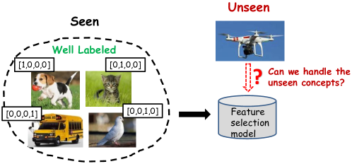
Figure 1: The Zero-Shot Feature Selection Problem.

Supervised knowledge (e.g., labels or pair-wise relationships) associated to data is capable of significantly improving the performance of feature selection methods [7]. However, it should be noted that existing supervised feature selection methods are facing an enormous challenge — the generation of reliable supervised knowledge cannot catch up with the rapid growth of newly-emerging concepts and multimedia data. In practice, it is costly to annotate sufficient training data for the new concepts timely, and meanwhile, impractical to retrain the feature selection model whenever a new concept emerges. As illustrated in Fig. 1, traditional methods perform well on the seen concepts which have correct guidance, but they may easily fail on the unseen concepts which have never been observed, like the newly invented product “quadrotor”. Therefore, the problem of Zero-Shot Feature Selection (ZSFS), i.e., building a feature selection model that generalizes well to unseen concepts with limited training data of seen concepts, deserves great attention. However, few studies have considered this problem.

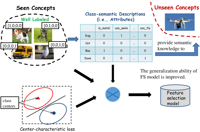
Figure 2: Overview of the proposed method.

The major challenge in the ZSFS problem is how to deduce the knowledge of unseen concepts from seen concepts. In fact, the primary reason why existing studies fail to handle unseen concepts is that they only consider the discrimination among seen concepts (like the 0/1-form class labels illustrated in Fig. 1), such that little knowledge could be deduced for unseen concepts. To address this, as illustrated in Fig. 2, we adopt the class-semantic descriptions (i.e., attributes) as supervision for feature selection. This idea is inspired by the recent development of Zero-Shot Learning (ZSL) [13] [1] [18] which has demonstrated that the capacity of inferring attributes allows us to describe, compare, or even categorize unseen objects.

An attendant problem is how to identify reliable discriminative features with attributes which might be inaccurate and noisy [17]. To alleviate this, we further propose a novel loss function (named center-characteristic loss) which encourages the selected features to capture the central characteristics of seen concepts. Theoretically, this loss function is a variant of the center loss [34] which has shown its effectiveness to learn discriminative and generalized features for categorizing unseen objects.

We evaluate the performance of the proposed method on several real-world datasets, including SUN, aPY and CIFAR10. One point should be noted is that the attributes of CIFAR10 are automatically generated from a public Wikipedia text-corpus [31] by a well-known NLP tool [16]. The experimental evidence shows that no matter with manually or automatically generated attributes, our method generalizes well to unseen concepts.

We summarize our main contributions as follows:

• We study the problem of ZSFS, i.e., building a feature selection model which generalizes well to unseen concepts with limited training data of seen concepts. To our best knowledge, little work has addressed this problem.

• We propose an efficient strategy to reuse the supervised knowledge of seen concepts. Concretely, feature selection is guided by the seen concept attributes which provide discriminative information about unseen concepts.

• To select more reliable discriminative features, we further encourage the selected features to capture the central characteristics of seen concepts. We formulate this by a novel loss function named center-characteristic loss.

• We conduct extensive experiments on three benchmark datasets to demonstrate the effectiveness of our method.

The rest of this paper is organized as follows. In Section 2, we briefly review some related work in feature selection and zero-shot learning. In Section 3, we formally define the problem studied in this paper. In Section 4, we elaborate our approach with details, together with the optimization method. In Section 5, more analysis of the method is provided. Extensive experiments on several different datasets will be reported in Section 6, followed by the conclusion in Section 7.

2 Related Work

2.1 Feature Selection

Feature selection, which selects a subset of the original features according to some criteria, plays an important role in pattern recognition and machine learning systems. In terms of the label availability, existing feature selection methods can be roughly classified into three groups: unsupervised, supervised and semi-supervised feature selection methods. In the unlabeled case, unsupervised methods select features which best keep the intrinsic structure of data according to various criteria, such as data variance [9], data similarity [26, 8] and data separability [4]. To take advantage of labeled data, supervised methods [22, 5, 37] evaluate features by their relevance to the given class labels. Extended from unsupervised and supervised methods, semi-supervised methods [19, 35, 36] utilize both labeled and unlabeled data to mine the feature relevance.

It should be noted that traditional feature selection methods do not consider the generalization to “unseen” concepts, limiting in the “seen” area where every concept should at least provide one (unlabeled or labeled) instance. In light of the knowledge explosion, with the rapid growth of newly-emerging concepts and multimedia data, building a feature selection model that generalizes well to unseen concepts has practical importance.

2.2 Attribute-based Zero Shot Learning

The task of Zero Shot Learning (ZSL) [21, 13, 1] is to recognize unseen objects without any label information. To achieve this goal, it leverages an intermediate semantic level (i.e., attribute layer) which is shared in both seen and unseen concepts. Take the seen concepts in Fig. 2 as an example. We can define some attributes like “can swim”, “can fly” and “is metal”. Then, we can train attribute recognizers using images and attribute information from seen concepts. After that, given an image belonging to unseen concepts, these attribute recognizers can infer the attributes of this image. Finally, the recognition result is obtained by comparing the test image’s attributes with each unseen concept’s attributes.

Although various ZSL methods have been proposed recently, they are mainly limited to classification or prediction applications. To our best knowledge, this is the first study to consider the zero-shot setting in the feature selection problem.

3 Problem Definition and Notations

Suppose there is a set of instances $X{=}\{x_{1},...,x_{n}\}^{\prime}\in\mathbb{R}^{n\times d}$ belonging to a seen concept set $\mathcal{C}$, where $x_{i}\in\mathbb{R}^{d}$ is the feature vector and $n$ is the instance number. We denote $Y{=}\{y_{1},...,y_{n}\}^{\prime}\in\{0,1\}^{n\times c}$ as the binary label indicator matrix, where $y_{i}\in\{0,1\}^{c}$ is the label vector of instance $x_{i}$ and $c$ is the number of seen concepts in $\mathcal{C}$.

Different from the traditional supervised feature selection setting where training and testing instances all belong to the same seen concept $\mathcal{C}$, the problem of Zero-Shot Feature Selection (ZSFS) considers a more challenging setting where testing instances belong to a related but “unseen” concept set $\mathcal{C}^{u}$. In other words, training and testing instances share no common concepts: $\mathcal{C}\cap\mathcal{C}^{u}{=}\varnothing$. Using only the training instances $X$ belonging to the seen concepts in $\mathcal{C}$, our goal is to learn a feature selection model that generalizes well to the unseen concepts in $\mathcal{C}^{u}$.

4 The Proposed Method

In this section, we provide a detailed description of the proposed method. Firstly, we discuss the feasibility of deducing knowledge of unseen concepts from seen concepts. Then, we describe the formulation of our method. Finally, we provide an effective solution to address the involved optimization issue.

4.1 Deduce Knowledge for Unseen Concepts

The success of ZSL demonstrates that the capacity of inferring attributes allows us to describe, compare, or even categorize unseen objects. Taking the seen concepts in Fig. 2 as an example, with the training images of these concepts, we could learn a mapping function between image features and some attributes (e.g., “has stripes”, “can fly” and “is metal”). As such, we can infer the attributes of the objects belonging to unseen concepts such as “koala” and “quadrotor”, so as to classify them without any training examples.

In light of this, as illustrated in Fig. 2, we propose to replace the original class labels with class-attribute descriptions (i.e., attributes) to guide feature selection. Unlike the original class labels (e.g., the 0/1-form label vectors in Fig. 1) which only reflect the discrimination among seen concepts, attributes provide additional semantic information about unseen concepts, making the feature selection models trained with seen concepts generalize well to unseen concepts. In other words, by introducing attributes, we can deduce the knowledge of unseen concepts from seen concepts. In the subsequent part, we denote this kind of semantic knowledge as $Y_{s}=[y^{s}_{1},...,y^{s}_{n}]^{\prime}\in\mathbb{R}^{n\times m}$, where $y^{s}_{i}\in\mathbb{R}^{m}$ denotes the attributes of the seen concept which instance $x_{i}$ belongs to, and $m$ is the attribute number. These attributes can either be provided manually or generated automatically from online textual documents [30, 28], such as Wikipedia articles.

4.2 Zero-Shot Feature Selection

4.2.1 Feature selection with attributes

We use $s{=}\{0,1\}^{d}$ as the indicator vector, where $s_{i}$=$1$ if the $i$-th feature is selected and $s_{i}$=$0$ otherwise. Denoting $\mathrm{diag}(s)$ as the matrix with the main diagonal being $s$, the original data can be represented as $X\mathrm{diag}(s)$ with the selected features. From a generative point of view, we assume that the selected features should have the ability to generate the given attributes. For simplicity and efficiency, we use a linear generating function $W{\in}\mathbb{R}^{d\times m}$, and adopt the squared loss to measure the error. Therefore, the optimal $s$ can be obtained by solving the following minimization problem:

$$\underset{W,s}{\text{min }} \mathcal{J}_{1}=\left\|Y_{s}-X\mathrm{diag}(s)W\right\|^{2}_{F}+\gamma\left\|W\right\|^{2}_{F}$$ (1)

$$\mathrm{s.t.} \hskip 5.0pts\in\{0,1\}^{d},\ s^{T}\textbf{1}_{d}=k$$

where $k$ is the number of features to select, $\gamma$ is the regularization parameter to avoid overfitting, and $\textbf{1}_{d}$ is a column vector with all its elements being 1. The most important part of Eq. 1 is the attributes $Y_{s}$ through which the power of categorizing unseen objects is captured by the selected features.

4.2.2 The center-characteristic loss

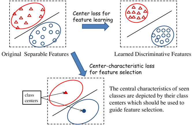
Figure 3: Center loss vs. Center-characteristic loss.

Although introducing attributes seems to be an effective solution for the ZSFS problem, it still has some limitations for discriminative feature selection. In particular, attributes cannot naturally describe the uncertainty about a class whose appearance may vary significantly [29]. For instance, “televisions” may have different colors and look quite differently from different angles. Moreover, attributes, which can be seen as real-valued multi-labels, tend to be more noisy than the common single-class labels [17]. For example, it is hard to determine a proper score for the attribute “running fast” for different animals and man-made vehicles.

Recent work [34] has pointed out that discriminative features are more generalized for identifying unseen objects than separable features. Specifically, to learn discriminative features, the work in [34] introduces center loss to minimize the distances between the learned features and their corresponding class centers (as illustrated in the upper portion of Fig. 3). Accordingly, for the feature selection task, this loss minimizes the distances between the selected features and their corresponding class centers, which yields the following minimization problem:

$$\underset{s}{\text{min }} \mathcal{J}_{2}=\left\|X\mathrm{diag}(s)-\bar{X}\mathrm{diag}(s)\right\|^{2}_{F}$$ (2)

$$\mathrm{s.t.} \hskip 5.0pts\in\{0,1\}^{d},\ s^{T}\textbf{1}_{d}=k$$

where $\bar{X}=\{\bar{x}_{1},...,\bar{x}_{n}\}^{\prime}\in\mathbb{R}^{n\times d}$, and $\bar{x}_{i}$ denotes the feature vector of the $y_{i}$-th class center.

However, this constraint may be too strict for a feature selection task, since all features are pre-calculated. On the other hand, as our ultimate goal is to find the relevance between features and attributes, it is reasonable to incorporate the attributes into this loss function. Therefore, we modify this constraint by multiplying the terms in the square loss with the generating function $W$ and approximate $X\mathrm{diag}(s)W$ with $Y_{s}$ according to Eq. 1. After this modification, Eq. 2 becomes:

$$\underset{W,s}{\text{min }} \mathcal{J}_{2}=\left\|Y_{s}-\bar{X}\mathrm{diag}(s)W\right\|^{2}_{F}$$ (3)

$$\mathrm{s.t.} \hskip 5.0pts\in\{0,1\}^{d},\ s^{T}\textbf{1}_{d}=k$$

We call this loss function center-characteristic loss, as it encourages the selected features to capture the central characteristics of seen concepts (illustrated in the lower portion of Fig. 3).

4.2.3 Zero-Shot feature selection joint learning model

By combining the objective functions in Eqs. 1 and 3, the proposed method is to solve the following optimization problem:

$$\underset{W,s}{\text{min }} \mathcal{J}=\left\|Y_{s}{-}X\mathrm{diag}(s)W\right\|^{2}_{F}{+}\alpha\left\|Y_{s}{-}\bar{X}\mathrm{diag}(s)W\right\|^{2}_{F}$$ (4)

$$\hskip 18.00003pt+\gamma\left\|W\right\|^{2}_{F}$$

$$\mathrm{s.t.} \hskip 4.5pts\in\{0,1\}^{d},\ s^{T}\textbf{1}_{d}=k$$

where $\alpha$ is a balancing parameter. We call the proposed method as Semantic based Feature Selection (SemFS), since we exploit the semantic knowledge (i.e., attributes) of seen concepts for the ZSFS problem.

Note that our method can be extended to handle both seen and unseen concepts, if we (just like the traditional feature selection methods) incorporate the original class labels into the final objective function. We leave this extension as future work.

4.3 Optimization

The optimization problem in Eq. 4 is a ‘0/1’ integer programming problem, which might be hard to solve by conventional optimization tools. Therefore, in this subsection, we give an efficient solution for this problem. First of all, to make the optimization tractable, we relax this ‘0/1’ constraint by allowing $s$ to take real non-negative values. This relaxation yields the following optimization problem:

$$\underset{W,s}{\text{min }} \mathcal{J}=\left\|Y_{s}{-}X\mathrm{diag}(s)W\right\|^{2}_{F}{+}\alpha\left\|Y_{s}{-}\bar{X}\mathrm{diag}(s)W\right\|^{2}_{F}$$ (5)

$$\hskip 18.00003pt+\gamma\left\|W\right\|^{2}_{F}$$

$$\mathrm{s.t.} \hskip 4.5pts\geq 0$$

As such, the objective function is differentiable w.r.t. the real-valued $s$. Intuitively, the value of $s_{i}$ can be interpreted as the importance score of $i$-th feature. Important features would have higher scores, while the scores of unimportant features tend to shrink towards 0. Therefore, after obtaining the solution of Eq. 5, we can rank $s$ to identify important features.

The optimization problem in Eq. 5 can be solved iteratively. Specifically, this consists of the following two steps.

Fix $s$ and update $W$

When $s$ is fixed, Eq. 5 is convex w.r.t $W$. Therefore, after removing the terms that are irrelevant to $W$, we can reformulate the objective function in Eq. 5 as the following unconstrained optimization problem:

$$\underset{W}{\text{min }} \mathcal{J}_{W}{=}\left\|Y_{s}{-}X\mathrm{diag}(s)W\right\|^{2}_{F}{+}\alpha\left\|Y_{s}{-}\bar{X}\mathrm{diag}(s)W\right\|^{2}_{F}$$ (6)

$$\hskip 18.00003pt+\gamma\left\|W\right\|^{2}_{F}$$

The derivative of $\mathcal{J}_{W}$ w.r.t. $W$ is:

$$\frac{\partial\mathcal{J}_{W}}{\partial W}=-2(X\mathrm{diag}(s))^{\prime}Y_{s}+2(X\mathrm{diag}(s))^{\prime}(X\mathrm{diag}(s))W$$ (7)

$$-2\alpha(\bar{X}\mathrm{diag}(s))^{\prime}Y_{s}{+}2\alpha(\bar{X}\mathrm{diag}(s))^{\prime}(\bar{X}\mathrm{diag}(s))W{+}2\gamma W$$

By setting this derivative to zero, we obtain the closed form solution for $W$:

$$W{=} [(X\mathrm{diag}(s))^{\prime}(X\mathrm{diag}(s)){+}\alpha(\bar{X}\mathrm{diag}(s))^{\prime}(\bar{X}\mathrm{diag}(s))$$ (8)

$${+}\gamma I_{d}]^{-1}[(X\mathrm{diag}(s))^{\prime}{+}\alpha(\bar{X}\mathrm{diag}(s))^{\prime}]Y_{s}$$

Fix $W$ and update $s$

When $W$ is fixed, the objective function in Eq. 5 can be rewritten as follows:

$$\underset{s}{\text{min }} \mathcal{J}_{s}{=}\left\|Y_{s}{-}X\mathrm{diag}(s)W\right\|^{2}_{F}{+}\alpha\left\|Y_{s}{-}\bar{X}\mathrm{diag}(s)W\right\|^{2}_{F}$$ (9)

$$\mathrm{s.t.} \hskip 4.5pts\geq 0$$

The derivative of $\mathcal{J}_{s}$ w.r.t. $s$ is:

$$\frac{\partial\mathcal{J}_{s}}{\partial s} =[-2X^{\prime}Y_{s}W^{\prime}+2X^{\prime}X\mathrm{diag}(s)WW^{\prime}$$ (10)

$$-2\alpha\bar{X}^{\prime}Y_{s}W^{\prime}+2\alpha\bar{X}^{\prime}\bar{X}\mathrm{diag}(s)WW^{\prime}]_{diag}$$

where $[\cdot]_{diag}$ denotes the vector of diagonal elements of matrix $[\cdot]$. In addition, since we require $s$ to be non-negative, we perform Projected Gradient Descent (PGD) [6] for this constrained optimization problem. Specifically, we project $s$ to be non-negative after each gradient updating step:

$$\mathrm{Proj}(s_{i})=max(0,s_{i}),\forall i=1,...,d$$ (11)

In summary, we can alternatively perform the above two steps until it converges or reaches a user-specified maximum iteration number. For clarity, we summarize this optimization procedure in Alg. 1.

Algorithm 1 Semantic based Feature Selection (SemFS)

1:Seen concept instances $X$ and attributes $Y_{s}$; Parameters $\alpha$ and $\gamma$;

2:Top ranked features for unseen concepts;

3:Calculate the center of each seen concept $\bar{X}$ ;

4:repeat

5:     Update $W$ by Eq. 8;

6:     Update $s$ through performing projected gradient descent by Eq. 10;

7:until Convergence or a certain iterations;

8:Rank features according to $s$ in a descending order and return the top ranked features.

5 Algorithm Analysis

5.1 Convergence Study

Proposition 1

At each iteration of Alg. 1, the objective value of Eq. 5 decreases until convergence.

Proof 1

As shown in Alg. 1, in each iteration, we update $W$ and $s$ in an alternative way. First of all, when $s$ is fixed, the original optimization problem (i.e., Eq. 5) w.r.t. $W$ reduces to the classical least square problem [11]. It can be easily verified that Eq. 8 is the optimal solution of this subproblem.

On the other hand, the update of $s$ is known as the projected gradient method which is guaranteed to converge to the minimum with appropriate choice of step size [24]. Therefore, Alg. 1 monotonically decreases the objective function value. In addition, since the objective function has a lower-bound of 0, Alg. 1 converges.

5.2 Time Complexity

Lines 3 and 4 in Alg. 1 list two main operations of our method, and the time complexity of each operation could be computed as:

• Line 3: Updating $W$ involves a matrix inversion and several matrix multiplications, and the total time complexity is $O(d^{3}+d^{2}n+dmn)$.

• Line 4: Updating $s$ also involves some matrix multiplications, and the time complexity is $O(dmn+d^{2}m+d^{2}n)$.

Generally speaking, the feature number and attribute number are much less than the seen instance number, i.e., ${d,m}\ll n$. Therefore, the total time complexity of each iteration in Alg. 1 is $\#iterations*O(n)$. As our method empirically converges quickly (usually in less than 20 iterations in our experiments), the overall time complexity of SemFS is linear to seen instance number $n$.

Note that if the feature number is large, the matrix inversion in Line 3 could be very time consuming. According to [25], this operation can be efficiently obtained through solving the following linear equation:

$$AW{=}[(Xdiag(s))^{\prime}{+}\alpha(\bar{X}diag(s))^{\prime}]Y_{s}$$ (12)

where $A{=}(Xdiag(s))^{\prime}(Xdiag(s)){+}\alpha(\bar{X}diag(s))^{\prime}(\bar{X}diag(s))\\ {+}\gamma I_{d}$. As such, the time complexity of Line 3 would be reduced to $O(md^{2}+d^{2}n+dmn)$.

5.3 SemFS v.s. Traditional Feature Selection Methods

Traditional feature selection methods including both unsupervised and (semi-)supervised methods all exploit the knowledge of seen concepts rather than unseen concepts [7]. Specifically, unsupervised methods generally prefer the features best preserving the intrinsic structure of seen concept data. (Semi-)supervised methods prefer the features best reflecting the discrimination (i.e., class labels) among different seen concepts. Consequently, as the data may vary dramatically among totally different concepts, traditional methods may not generalize well to unseen concepts.

Conversely, our method prefers the features best reflecting the knowledge about the attributes of seen concepts. As it is practicable to categorize unseen objects via inferring attributes, the selected features in our method would also have this ability, which is further verified in our later experiments.

6 Experiments

Table 1: The statistics of datasets

	SUN	aPY	CIFAR10
# seen concepts	707	20	2
# seen images	14,140	12,695	12,000
# unseen concepts	10	12	8
# unseen images	200	2,644	48,000
# attributes	102	64	50
# features	4,096	4,096	4,096

6.1 Experimental Setup

Datasets

The experiments are conducted on three widely used benchmark datasets. The first dataset is SUN scene attributes database (SUN) [27] which contains 14,340 images from 717 different scenes like “village” and “airport”. For each image, a 102-dimensional binary attribute vector is annotated manually. We average the images’ attributes to obtain the attributes for each concept, and follow the seen/unseen split setting as [17].

The second dataset is aPascal/aYahoo objects dataset (aPY) [13] which contains two subsets. The aPascal subset comes from PASCAL VOC2008 dataset, and contains 20 different categories, such as “people” and “dog”. The aYahoo subset is collected by Yahoo image search engine, and has 12 similar but different categories compared to aPascal, such as “monkey” and “zebra”. This dataset has a standard split setting, i.e., aPascal and aYahoo serve as the seen part and unseen part respectively. Each image is annotated by a 64-dimensional binary attribute vector. We average the attribute vectors of images in the same category to get the class attributes.

The third dataset is CIFAR10 [20] which consists of 10 classes of objects with 6,000 images per class. Since this dataset does not have a standard seen/unseen split setting, we randomly adopt two classes as seen. Thus, we have $C_{10}^{2}$ different seen/unseen splits. The purpose of this setting is to test the extreme case where most of the concepts are unseen. In addition, as this dataset does not have any attribute annotations, we adopt the 50-dimensional word vector provided by [16] as attributes for each class. Concretely, these embedding vectors are automatically generated from a Wikipedia corpus [31] with a total of about 2 million articles and 990 million tokens.

For all these three datasets, we use the widely used 4,096-dimensional deep features provided by [14]. The detailed statistics of these three benchmarks are listed in Table 1.

6.1.1 Comparison methods

We compare the proposed method SemFS with both unsupervised and supervised feature selection methods:

1. Random method selects features randomly.

2. MCFS [4] is an unsupervised method selecting features by using spectral regression with $\ell_{1}$-norm regularization.

3. FSASL [10] is an unsupervised method performing structure learning and feature selection simultaneously.

4. LASSO [33] is the classical supervised feature selection method.

5. L20ALM [5] is a supervised method evaluating features under an $\ell_{21}$-norm loss function with $\ell_{20}$-norm constraint.

6. WkNN [3] is a newest supervised feature selection method based on k-nearest neighbors algorithm

In addition, to validate the effectiveness of the proposed center-characteristic loss, we test a variant of our method (denoted as SemFS/c) by setting $\alpha{=}0$ in Eq. 5 to eliminate the effect of this loss term. Another point to be noted is that we apply all methods on seen concepts and then evaluate the quality of selected features on unseen concepts. In other words, in the training phase, the unseen concepts are invisible to all methods.

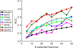
(a) SUN

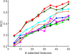
(b) aPY

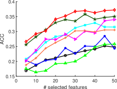
(c) CIFAR10

Figure 4: Clustering results (ACC).

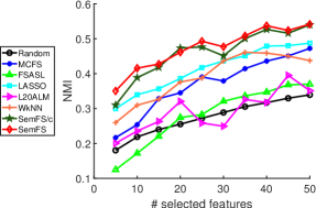
(a) SUN

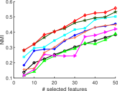
(b) aPY

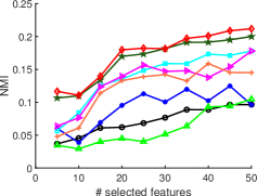
(c) CIFAR10

Figure 5: Clustering results (NMI).

6.1.2 Experimental Setting

Since determining the optimal number of selected features is still an open problem [32], we follow [10] to vary the selected features number from 5 to 50 in intervals of 5. As the unseen concepts have no labeled data, we evaluate the selected features on the clustering task, so as to follow the current practice of evaluating unsupervised feature selection [4]. Specifically, we employ the classical K-means clustering method and adopt two widely used clustering metrics, i.e., Accuracy (ACC) and Normalized Mutual Information (NMI) [12]. Since K-means is sensitive to initialization, we repeat the clustering 20 times with random initializations and report the average performance. To fully show the limitations of these compared methods, we tune their parameters by a grid-search strategy from $\{10^{-2},10^{-1},10^{0},10^{1},10^{2}\}$ and report the best results. In contrast, to show the effectiveness of our method, we simply fix our parameters $\alpha{=}1$ and $\gamma{=}0.1$ throughout the experiment.

6.2 Clustering with Selected Features

Figure 4 and Figure 5 show the clustering performance in terms of ACC and NMI, respectively. There are several important observations to be made.

• Our methods (both SemFS and SemFS/c) always outperform the others significantly, in terms of both ACC and NMI, on all datasets. For example, with 20 selected features, our two methods outperform the best baseline by 20–-40% relatively in terms of ACC. The underlying principle is that our methods successfully deduce the knowledge of unseen concepts from seen concepts by introducing attributes.

• An interesting observation is that the unsupervised method MCFS is comparable to or even better than those supervised baselines. This indicates that the supervised methods may be misled by the seen concept labels which provide little information about unseen concepts.

• On the CIFAR10 dataset where most concepts are unseen and attributes are automatically generated, our methods could still identify high quality features (Figs. 4(c) and 5(c)). This confirms the flexibility of our methods as well as the advantage of attributes.

• SemFS consistently obtains more stable and better performance than SemFS/c. This phenomenon indicates that the proposed center-characteristic loss can help to select reliable discriminative features for unseen concepts with limited labeled seen instances.

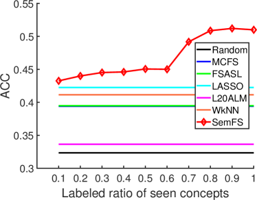
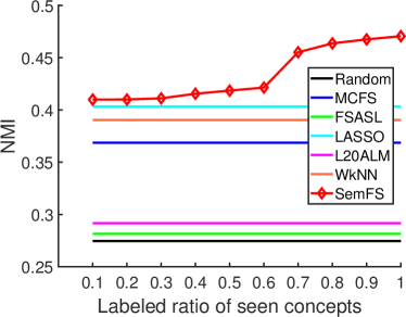
Figure 6: Average clustering performance w.r.t. different labeled ratios of seen concepts on SUN.

6.3 Effect of Labeled Seen Concept Ratio

In this part, we evaluate the performance of the proposed method SemFS w.r.t. the labeled ratio in all seen concepts. Specifically, in our method, we vary the labeled ratio of each seen concept from 0.1 to 1. Figure 6 shows the average clustering performance on SUN (due to space limitations, we do not report the results on the other datasets, because we have similar observations on them). It can be observed that even with only 10% of seen concepts, SemFS could still benefit the success of cross-concept knowledge generalization. This verifies the superiority of attributes for the ZSFS problem. On the other hand, we find that as labeled ratio of seen concepts increases, our method shows an increasing advantage over the previous studies. We analyse that with more seen concepts, SemFS would deduce more reliable supervision for the unseen concepts, thereby simultaneously improving the quality of selected features.

6.4 Advantage of Attributes

To further show the advantage of attributes, we use three methods: SemFS, SemFS/c and the compared classical feature selection method LASSO. For clarity, we use $\mathcal{M}_{o}$ and $\mathcal{M}_{s}$ to denote the method $\mathcal{M}$ using the original class labels (i.e., $Y$) and semantic attributes (i.e., $Y_{s}$), respectively. Figure 7 shows the average clustering results in terms of ACC. It can be clearly observed that: compared to the original class labels, attributes could significantly improve the generalization ability of these feature selection methods. The underlying reason is that attributes contain discriminative information about unseen concepts. In contrast, the original class labels neglect this kind of knowledge, thereby leading to poor performance.

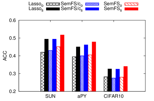
Figure 7: Average ACC: class labels vs. attributes.

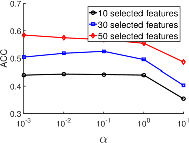
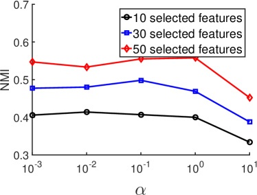
Figure 8: The effect of parameter $\alpha$ on SUN.

6.5 Parameter Sensitivity

In the proposed method SemFS, there is an important parameter $\alpha$ which controls the penalty of center loss. Figure 8 shows the clustering performance w.r.t. this parameter on SUN (with the fixed regularization parameter $\lambda{=}1$). It can be observed that our method is not very sensitive to $\alpha$, and the results remain almost the same when the parameters vary among $\{10^{-3},...,10^{0}\}$ in our experiments.

7 Conclusion

This paper investigates the problem of Zero-Shot Feature Selection, i.e., building a feature selection model that generalizes well to unseen concepts with limited training data of seen concepts. We propose a novel feature selection method named SemFS. The basic idea of our method is to guide feature selection by attributes which can be seen as a bridge for transferring supervised knowledge from seen concepts to unseen concepts. In addition, we propose the center-characteristic loss to enhance the quality of selected features. Finally, we formulate these two components into a joint learning model and give an efficient solution. Extensive experiments conducted on several real-world datasets demonstrate the effectiveness of our method. In the future, we plan to extend our method to use the additional unlabeled data of seen concepts.

References

- Akata et al. [2016] Akata, Z., Malinowski, M., Fritz, M., Schiele, B., 2016. Multi-cue zero-shot learning with strong supervision. In: Proceedings of the IEEE Conference on Computer Vision and Pattern Recognition. pp. 59–68.
- Bicciato et al. [2003] Bicciato, S., Luchini, A., Di Bello, C., 2003. Pca disjoint models for multiclass cancer analysis using gene expression data. Bioinformatics 19 (5), 571–578.
- Bugata and Drotár [2019] Bugata, P., Drotár, P., 2019. Weighted nearest neighbors feature selection. Knowledge-Based Systems 163, 749–761.
- Cai et al. [2010] Cai, D., Zhang, C., He, X., 2010. Unsupervised feature selection for multi-cluster data. In: Proceedings of the 16th ACM SIGKDD international conference on Knowledge discovery and data mining. ACM, pp. 333–342.
- Cai et al. [2013] Cai, X., Nie, F., Huang, H., 2013. Exact top-k feature selection via l2, 0-norm constraint. In: International Joint Conference on Artificial Intelligence (IJCAI). pp. 1240–1246.
- Calamai and Moré [1987] Calamai, P. H., Moré, J. J., 1987. Projected gradient methods for linearly constrained problems. Mathematical programming 39 (1), 93–116.
- Chandrashekar and Sahin [2014] Chandrashekar, G., Sahin, F., 2014. A survey on feature selection methods. Computers & Electrical Engineering 40 (1), 16–28.
- Chu and Zhao [2018] Chu, Y., Zhao, Y., 2018. Bidirectional feature selection with global and local structure preservation for small size samples. Cognitive Systems Research 52, 756–764.
- Dash and Liu [2000] Dash, M., Liu, H., 2000. Feature selection for clustering. In: Pacific-Asia Conference on knowledge discovery and data mining. Springer, pp. 110–121.
- Du and Shen [2015] Du, L., Shen, Y.-D., 2015. Unsupervised feature selection with adaptive structure learning. In: Proceedings of the 21th ACM SIGKDD International Conference on Knowledge Discovery and Data Mining. ACM, pp. 209–218.
- Duda et al. [1995] Duda, R. O., Hart, P. E., Stork, D. G., 1995. Pattern classification and scene analysis 2nd ed. ed: Wiley Interscience.
- Duda et al. [2012] Duda, R. O., Hart, P. E., Stork, D. G., 2012. Pattern classification. John Wiley & Sons.
- Farhadi et al. [2009] Farhadi, A., Endres, I., Hoiem, D., Forsyth, D., 2009. Describing objects by their attributes. In: Proceedings of the IEEE Conference on Computer Vision and Pattern Recognition. IEEE, pp. 1778–1785.
- Guo et al. [2016] Guo, Y., Ding, G., Gao, Y., Wang, J., 2016. Semi-supervised active learning with cross-class sample transfer. In: Proceedings of the Twenty-Fifth International Joint Conference on Artificial Intelligence. pp. 1526–1532.
- Guyon and Elisseeff [2003] Guyon, I., Elisseeff, A., 2003. An introduction to variable and feature selection. Journal of machine learning research 3 (Mar), 1157–1182.
- Huang et al. [2012] Huang, E. H., Socher, R., Manning, C. D., Ng, A. Y., 2012. Improving word representations via global context and multiple word prototypes. In: Proceedings of the 50th Annual Meeting of the Association for Computational Linguistics: Long Papers-Volume 1. pp. 873–882.
- Jayaraman and Grauman [2014] Jayaraman, D., Grauman, K., 2014. Zero-shot recognition with unreliable attributes. In: Advances in Neural Information Processing Systems. pp. 3464–3472.
- Ji et al. [2019] Ji, Z., Yu, X., Yu, Y., He, Y., 2019. Manifold embedding for zero-shot recognition. Cognitive Systems Research 55, 34–43.
- Kong and Yu [2010] Kong, X., Yu, P. S., 2010. Semi-supervised feature selection for graph classification. In: Proceedings of the 16th ACM SIGKDD international conference on Knowledge discovery and data mining. ACM, pp. 793–802.
- Krizhevsky and Hinton [2009] Krizhevsky, A., Hinton, G., 2009. Learning multiple layers of features from tiny images.
- Lampert et al. [2009] Lampert, C. H., Nickisch, H., Harmeling, S., 2009. Learning to detect unseen object classes by between-class attribute transfer. In: Proceedings of the IEEE Conference on Computer Vision and Pattern Recognition. IEEE, pp. 951–958.
- Lee Rodgers and Nicewander [1988] Lee Rodgers, J., Nicewander, W. A., 1988. Thirteen ways to look at the correlation coefficient. The American Statistician 42 (1), 59–66.
- Lin et al. [2018] Lin, Q., Xue, Y., Wen, J., Zhong, P., 2018. A sharing multi-view feature selection method via alternating direction method of multipliers. Neurocomputing.
- Luenberger and Ye [2015] Luenberger, D. G., Ye, Y., 2015. Linear and nonlinear programming. Vol. 228. Springer.
- Nie et al. [2010] Nie, F., Huang, H., Cai, X., Ding, C. H., 2010. Efficient and robust feature selection via joint l2, 1-norms minimization. In: Advances in neural information processing systems. pp. 1813–1821.
- Nie et al. [2008] Nie, F., Xiang, S., Jia, Y., Zhang, C., Yan, S., 2008. Trace ratio criterion for feature selection. In: AAAI. Vol. 2. pp. 671–676.
- Patterson and Hays [2012] Patterson, G., Hays, J., 2012. Sun attribute database: Discovering, annotating, and recognizing scene attributes. In: Proceedings of the IEEE Conference on Computer Vision and Pattern Recognition. IEEE, pp. 2751–2758.
- Qiao et al. [2016] Qiao, R., Liu, L., Shen, C., Hengel, A. v. d., 2016. Less is more: zero-shot learning from online textual documents with noise suppression. arXiv preprint arXiv:1604.01146.
- Ren et al. [2016] Ren, Z., Jin, H., Lin, Z., Fang, C., Yuille, A., 2016. Joint image-text representation by gaussian visual-semantic embedding. In: Proceedings of the 2016 ACM on Multimedia Conference. ACM, pp. 207–211.
- Rohrbach et al. [2010] Rohrbach, M., Stark, M., Szarvas, G., Gurevych, I., Schiele, B., 2010. What helps where–and why? semantic relatedness for knowledge transfer. In: Proceedings of the IEEE Conference on Computer Vision and Pattern Recognition. IEEE, pp. 910–917.
- Shaoul [2010] Shaoul, C., 2010. The westbury lab wikipedia corpus. Edmonton, AB: University of Alberta.
- Tang and Liu [2012] Tang, J., Liu, H., 2012. Unsupervised feature selection for linked social media data. In: Proceedings of the 18th ACM SIGKDD international conference on Knowledge discovery and data mining. ACM, pp. 904–912.
- Tibshirani [1996] Tibshirani, R., 1996. Regression shrinkage and selection via the lasso. Journal of the Royal Statistical Society. Series B (Methodological), 267–288.
- Wen et al. [2016] Wen, Y., Zhang, K., Li, Z., Qiao, Y., 2016. A discriminative feature learning approach for deep face recognition. In: European Conference on Computer Vision. Springer, pp. 499–515.
- Xu et al. [2010] Xu, Z., King, I., Lyu, M. R.-T., Jin, R., 2010. Discriminative semi-supervised feature selection via manifold regularization. IEEE Transactions on Neural networks 21 (7), 1033–1047.
- Zeng et al. [2016] Zeng, Z., Wang, X., Zhang, J., Wu, Q., 2016. Semi-supervised feature selection based on local discriminative information. Neurocomputing 173, 102–109.
- Zhao et al. [2018] Zhao, M., Lin, M., Chiu, B., Zhang, Z., Tang, X.-s., 2018. Trace ratio criterion based discriminative feature selection via l2, p-norm regularization for supervised learning. Neurocomputing 321, 1–16.