Out of Time Order Correlations in the Quasi-Periodic Aubry-André model

Abstract

We study out of time ordered correlators (OTOC) in a free fermionic model with a quasi-periodic potential. This model is equivalent to the Aubry-André model and features a phase transition from an extended phase to a localized phase at a non-zero value of the strength of the quasi-periodic potential. We investigate five different time-regimes of interest for out of time ordered correlators; early, wavefront, $x=v_{B}t$, late time equilibration and infinite time. For the early time regime we observe a power law for all potential strengths. For the time regime preceding the wavefront we confirm a recently proposed universal form and use it to extract the characteristic velocity of the wavefront for the present model. A Gaussian waveform is observed to work well in the time regime surrounding $x=v_{B}t$. Our main result is for the late time equilibration regime where we derive a finite time equilibration bound for the OTOC, bounding the correlator’s distance from its late time value. The bound impose strict limits on equilibration of the OTOC in the extended regime and is valid not only for the Aubry-André model but for any quadratic model. Finally, momentum out of time ordered correlators for the Aubry-André model are studied where large values of the OTOC are observed at late times at the critical point.

I Introduction

Recently out of time ordered correlators (OTOCs) have experienced a resurgence of interest from different fields of physics ranging from the black hole information problem Maldacena et al. (2016) to information propagation in condensed matter systems Yoshida (2019); Swingle and Chowdhury (2017); González Alonso et al. (2019); Yan et al. (2019); Tuziemski (2019); Mao et al. (2019); Lewis-Swan et al. (2019); Nakamura et al. (2019). The OTOC is of particular interest due to its role in witnessing the spreading or“scrambling” of locally stored quantum information across all degrees of freedom of the system, something traditional dynamical correlation functions of the form $\langle A(t)B\rangle$ cannot. Thus, thermalization must have information scrambling as a precursor since the thermal state necessarily will have lost information about any initial state, although thermalization typically occurs at a significantly longer time-scale Bohrdt et al. (2017). An upper bound for the initial exponential growth, $e^{\lambda_{L}t}$, of the OTOC, with $\lambda_{L}\leq 2\pi k_{B}T/\hbar$ has been conjectured Maldacena et al. (2016). Models approaching or saturating this bound are known as fast scramblers, in contrast to many condensed matter systems which exhibit a much slower growth and are therefore known as slow scramblers. The introduction of disorder significantly alters the information spreading, restricting it within a localization length in Anderson insulators Riddell and Sørensen (2019) and partially halting the growth of the OTOC in many-body localized states Swingle and Chowdhury (2017). The OTOC is directly related to the Loschmidt Echo Yan et al. (2019) and is has been established that the second Renyi entropy can be expressed in terms of a sum over appropriately defined OTOCs Fan et al. (2017). Any bound that can be established on the growth of the OTOC therefore implies a related bound on the entanglement. A further understanding of the dynamics of quantum information in models with both extended and localized states is therefore of considerable interest and our focus here is on understanding how this arises in the quasi-periodic Aubry-André (AA) model where a critical potential strength separates an extended and localized phase.

An OTOC is generally written in the form,

$$C(x,t)=\langle[\hat{A}(t),\hat{B}]^{\dagger}[\hat{A}(t),\hat{B}]\rangle,$$ (1)

where $\hat{A}$, $\hat{B}$ are local observables which commute at $t=0$. If the observables are both hermitian and unitary the OTOC can be re-expressed as,

$$C(x,t)=2-2\Re[F(x,t)],$$ (2)

where,

$$F(x,t)=\langle\hat{A}(t)\hat{B}\hat{A}(t)\hat{B}\rangle.$$ (3)

Often one refers to both $F$ and $C$ as the OTOC. From a condensed matter perspective the OTOC is a measure of an operator spreading its influence over a lattice, and quantifies the degree of non-commutativity between two operators at different times. If the initially zero $C(x,t)$ remains non-zero for an extended period of time we say the system has scrambled. A closely analogous diagnostic tool, capable of detecting information scrambling, can be defined in terms of the mutual information between two distant intervals Alba and Calabrese (2019).

From a measurement perspective $F(x,t)$ can be understood as a series of measurements. First acting on the state with operator $\hat{B}$ at $t=0$ and evolving in time to $t>0$, then acting on the state with operator $\hat{A}$, then evolving for time $-t<0$. The OTOC is then obtained by calculating the overlap between the resulting state and the state that is first evolved by $t$, then acted upon by $A$, then evolved by $-t$ and finally acted upon by $B$. Typically in the context of the OTOC one uses $\langle\dots\rangle$ as the thermal average, often at infinite temperature, but studies in a non-equilibrium setting starting from product states have also been done Lee et al. (2018); Riddell and Sørensen (2019); Chen et al. (2017). Out of time correlators have also sparked experimental interest and significant progress has been made to reliably measure these quantities Swingle et al. (2016); Zhu et al. (2016); Yao et al. (2016); Danshita et al. (2017); Gärttner et al. (2017). The correlators have even been reliably simulated on a small quantum computer Li et al. (2017a) and recently on an ion trap quantum computer Landsman et al. (2019).

The dynamics of the OTOC has five important regimes; early time, the wavefront, $x=v_{B}t$, late time dynamics and the infinite time limit. The early time growth of OTOCs has been of interest as an initial growth of the OTOC that precedes classical information. If the Hamiltonian is local in interactions then use of the Hadamard formula (see ref. Miller (1972) lemma 5.3) allows one to conclude that in the early time regime the OTOC grows with a power law in time,

$$C(x,t)\sim t^{l(x)},$$ (4)

where $t$ is small and $l(x)$ is a linearly increasing function of the distance. The early power law growth in time occurs before the wavefront hits and is known to be independent of the integrability of the model Dóra and Moessner (2017); Roberts and Swingle (2016); Chen et al. (2018); Lin and Motrunich (2018); Riddell and Sørensen (2019); Lee et al. (2018); Bao and Zhang (2019). This polynomial form is also known to be independent of disorder strength and has been observed to hold in localized regimes Riddell and Sørensen (2019); Lee et al. (2018).

More interestingly, the wavefront tracks the passage of classical information in the system. A universal wavefront form has been proposed Xu and Swingle (2018a); Khemani et al. (2018), valid for $t\ll x/v_{B}$,

$$C(x,t)\sim\exp\left(-\lambda_{L}\frac{(x-v_{B}t)^{1+p}}{t^{p}}\right),$$ (5)

where $\lambda_{L}$ is the Lyapunov exponent and $v_{B}$ is the butterfly velocity. Several other forms have been proposed, for a review see Ref. Xu and Swingle (2018a). The above wavefront form, Eq. (5), has been confirmed in several cases, and even used to show a chaotic to many body localization transition Nahum et al. (2018); von Keyserlingk et al. (2018); Jian and Yao (2018); Gu et al. (2017); Xu and Swingle (2018b, a); Khemani et al. (2018); Sahu et al. (2018); Rakovszky et al. (2018); Shenker and Stanford (2014); Patel et al. (2017); Chowdhury and Swingle (2017); Jian and Yao (2018). For free models one can show with a saddle point approximation that the form from Eq. (5) takes $p=\frac{1}{2}$ and $v_{B}$ is the maximal group velocity of the model Xu and Swingle (2018b, a); Khemani et al. (2018). A particular appealing feature of Eq. (5) is the appearance of a well-defined Butterfly velocity, $v_{B}$ for a large range of models. A recent numerical study focusing on the random field XX-model suggested that for this disordered model a different form could be made to fit better over an extended region Riddell and Sørensen (2019) surrounding $x=v_{B}t$. This result suggests further studies are important for understanding how quantum information is spreading through the system.

The late time dynamics of OTOCs are a similarly rich regime of interest. Understanding how the function $g(t)=|C(x,t)-C(x,t\to\infty)|^{2}$ decays in time has received attention in many models. In the case of the anisotropic XY model the decay of the OTOC to its equilibrium value is an inverse power law Lin and Motrunich (2018); Bao and Zhang (2019),

$$C(x,t)\sim\frac{1}{t^{\alpha}}+\gamma,$$ (6)

where $\alpha\geq 0$ depending on the choices of spin operators and the anisotropy, and $\gamma$ is the equilibrium value. Other work has been done on interacting systems where both inverse power laws were observed for chaotic and many body localized phases, and even an exponential decay in time for Floquet systems Chen et al. (2017); Swingle and Chowdhury (2017). However, these results are mostly numerical, and do not give rigorous bounds or arguments as to whether or not the OTOC reaches equilibrium and if it does, to what resolution. Another aspect of the late time regime, the quantity $C(x,t\to\infty)$ in it self, is naturally of considerable interest. In this setting $F(x,t\to\infty)$ is often chosen as the quantity to study. In the presence of chaos we expect $F$ to equilibrate to zero, and in other cases settle at a finite value between zero and one Huang et al. (2017a); Fan et al. (2017); Chen (2016a); Swingle and Chowdhury (2017); He and Lu (2017); Riddell and Sørensen (2019); Lin and Motrunich (2018); Bao and Zhang (2019); Chen et al. (2017); Lee et al. (2018); Roberts and Yoshida (2017); Huang et al. (2017b); Chen (2016b); Max McGinley (2018). A particularly important case for our purposes are the non-interacting models where the observables defining the OTOC are both local in fermionic and spin representations on the lattice. Here $F(x,t)$ is expected to initially decay towards zero, but eventually return to $F(x,t)=1$ and in the presence of disorder need not decay back to its initial value or even equilibrate Bao and Zhang (2019); Riddell and Sørensen (2019); Lin and Motrunich (2018); Chen (2016a); Max McGinley (2018). Of course, $C$ is then predicted to follow the opposite behaviour, starting at zero then reaching a maximum. It is also noteworthy that, in the proximity of a quantum critical point the OTOC has been shown to follow dynamical scaling laws Wei et al. (2019).

The introduction of disorder, with the potential of leading to localization, significantly changes the behaviour of the OTOC and propagation of quantum information as a whole. Naturally, quantum information dynamics is expected to be dramatically different between localized and extended phases. We therefore focus on the one-dimensional quasiperiodic Aubry-André (AA) model Aubry and André (1980); Hiramoto and Kohmoto (1989):

$$H=-\frac{J}{2}\sum_{j}(|j\rangle\langle j+1|+\mathrm{h.c})+\lambda\sum_{j}\cos(2\pi\sigma j)|j\rangle\langle j|.$$ (7)

Here, $J$ is the hopping strength and $\lambda$ the strength of the quasi-periodic potential. This model has been extensively studied Aulbach et al. (2004); Boers et al. (2007); Modugno (2009); Albert and Leboeuf (2010); Ribeiro et al. (2013); Danieli et al. (2015); Wang and Tong (2017); Li et al. (2017b); Martínez et al. (2018); Castro and Paredes (2019) and since it is quadratic large-scale exact numerical results can be obtained from the exact solution. In particular quench dynamics has recently been studied Gramsch and Rigol (2012). Crucially, it is well established that a critical potential strength $\lambda_{c}=J$ separates an extended and localized regime if $\sigma$ is chosen to be the golden mean $\sigma=(\sqrt{5}-1)/2$. For finite lattices this strictly only holds if the system size is chosen as $L=F_{i}$, with $F_{i}$ a Fibonacci number, and $\sigma=F_{i-1}/F_{i}$ approaching the golden mean as $i\to\infty$. A dual model can then be formulated Aubry and André (1980); Aulbach et al. (2004) by introducing the dual basis $|\bar{k}\rangle=L^{-1/2}\sum_{j}\exp(i2\pi\bar{k}\sigma j)|j\rangle$. $\lambda_{c}=J$ is then the self-dual point. The extended phase is characterized by ballistic transport as opposed to diffusive Aubry and André (1980). The nature of the quasi-periodic potential is also special since no rare regions exists and it has recently been argued that localization in the AA model is fundamentally more classical than disorder-induced Anderson localization Albert and Leboeuf (2010). It is possible to realize this model quite closely in optical lattices and studies of both bosonic and fermionic experimental realizations have been pursued using ³⁹K bosons Roati et al. (2008); Deissler et al. (2010); Lucioni et al. (2011), ⁸⁷Rb bosons Fallani et al. (2007), and ⁴⁰K fermions Schreiber et al. (2015); Lüschen et al. (2017a, b).

The AA model has also recently been studied in the presence of an interaction term Iyer et al. (2013); Xu et al. (2019). While no longer exactly solvable, a many-body localized phase can be identified in studies of small chains Iyer et al. (2013); Xu et al. (2019) and by analyzing the OTOC it has been suggested that an intermediate ’S’ phase occurs between the extended and many-body localized phases with a power-law like causal lightcone Xu et al. (2019).

The structure of this paper is as follows, in section II we discuss our formulation of the Aubry-André model and describe the quench protocol we use. In section III we investigate the dynamics of an out of time ordered correlator in real space and break the section into three subsections dedicated to three dynamical regions of interest. In subsection III.1 we show that when quenching into either the extended, localized, or critical phase a power-law growth is observed in the early time regime. In III.2 we investigate the discrepancies between Xu and Swingle (2018a); Khemani et al. (2018) and Riddell and Sørensen (2019) for times closer to the wave-front. Section III.3 contains a proof that, in the extended phase of a free model, we expect the out of time ordered correlator to equilibrate even in the presence of the quasi-periodic potential. The infinite time value is also shown to be zero regardless of the strength of the quasi-periodic potential indicating a lack of scrambling regardless of disorder in the extended phase. Finally in section IV we investigate OTOCs constructed from momentum occupation operators and find that they obey a simple waveform.

II The model and OTOCs

As outlined, we focus on the quasi-periodic AA model. We chose a fermionic representation and write the Hamiltonian as follows:

$$\hat{H}=\sum_{i,j}M_{i,j}\hat{f}_{i}^{\dagger}\hat{f}_{j},$$ (8)

where the effective elements of the Hamiltonian matrix $M$ is filled by, $M_{i,j}=-\frac{J}{2}$ if $|i-j|=1$ and $M_{j,j}=\lambda\cos(2\pi\sigma j)$. The operators are fermionic so we have $\{\hat{f}_{k},\hat{f}_{l}\}=\{\hat{f}_{k}^{\dagger},\hat{f}_{l}^{\dagger}\}=0$ and $\{\hat{f}_{l}^{\dagger},\hat{f}_{k}\}=\delta_{l,k}$. All other entries of the effective Hamiltonian are zero. Note that this corresponds to open boundary conditions with nearest neighbour hopping which is the most convenient for the calculations. The constant $\sigma$ is the inverse golden ratio, $\sigma=(\sqrt{5}-1)/2$. For the very large system sizes we use we have not been able to observe any numerical difference between using $L=F_{i},\ \sigma=F_{i-1}/L$ and using a large $L$ with $\sigma=(\sqrt{5}-1)/2$ even though the model is strictly no longer self-dual. For convenience we therefore use the latter approach. Since the inverse golden ratio is irrational, this creates a quasi-periodic potential controlled by the value of $\lambda$. For the rest of our discussion we set $J=1$ and $\hbar=1$. This model is identical to the Aubry-André model as can be seen through a series of transformations Aubry and André (1980); Coleman (2015). One can easily diagonalize and time evolve states in this model, the details of which are presented in the Appendix A. As described above, this model is known to have a localization transition at a critical point $\lambda_{c}=J$. For $\lambda<\lambda_{c}$ all states are extended, and $\lambda>\lambda_{c}$ all states are localized with localization length $\xi=\frac{1}{\ln\lambda}$ Aubry and André (1980). Relaxation and thermalization following a quench into both extended and localized phases has recently been investigated in this model Gramsch and Rigol (2012). While most one-body observables thermalize to a generalized Gibbs ensemble in the extended state, and some in the localized, special dynamics was observed for a quench to the critical points where the observables investigated did not reach a clear stationary value in the time intervals investigated. Similar quadratic fermionic models have been used to investigate OTOCs at large system sizes, showing non-trivial behaviour of both non-disordered and disordered OTOC investigations in integrable models Riddell and Sørensen (2019); Lin and Motrunich (2018); Muralidharan et al. (2018).

The OTOCs we will be interested in are written in the form Eq. (1) where we choose $\hat{A}$ and $\hat{B}$ such that they commute at $t=0$ and are unitary. The operators being hermitian and unitary then obey Eq. (2), (3). In general we choose our operators such that at $t=0$ $[\hat{A},\hat{B}]=0$, making $C(x,0)=0$ in all cases. This gives us a convenient reference point in time. Because we are talking about fermionic operators, it makes sense to only consider operators which are quadratic, and further, we choose to restrict ourselves to operators that can be expressed as number operators in real or momentum space. In momentum space the operators we consider are :

$$\eta_{k}:=\frac{1}{\sqrt{L}}\sum_{j}e^{ikj}\hat{f}_{j}$$ (9)

$$\eta_{k}^{\dagger}:=\frac{1}{\sqrt{L}}\sum_{j}e^{-ikj}\hat{f}_{j}^{\dagger}.$$ (10)

Where, $k\in 2\pi m/L$ with $m=1,2\dots L$. These operators are extremely non-local in the real space operators, and for the case of $\lambda=0$ and periodic boundary conditions, are the operators which diagonalize $M$ (strictly speaking only when periodic boundary conditions are used). It has been observed previously that operators not local in the fermionic representation show fundamentally different behaviour than the local ones Lin and Motrunich (2018). These however were spin operators, which were non-local in the Jordan-Wigner transform, so investigating OTOCs with momentum number operators is not entirely an exact analogue.

III Real space OTOCs

We start by considering OTOCs based on operators defined in real space. To be specific we study the following operators,

$$\hat{A}(t)=2\hat{f}_{\frac{L}{2}}^{\dagger}(t)\hat{f}_{\frac{L}{2}}(t)-1\enspace\text{,}\enspace\hat{B}=2\hat{f}_{j}^{\dagger}\hat{f}_{j}-1$$ (11)

Where we have fixed the location of $\hat{A}$ in space at the middle point of the lattice, and we will vary the location of $\hat{B}$, so we see can observe the effect of $\hat{A}$ spreading over the lattice. The operators are written with a factor of $2$ and a subtraction of $1$ to make them unitary. The dynamics and calculations of the OTOC in this setting is presented in Appendix A, B and C.

III.1 Early time

In this section we explore the early time behavior of the real space OTOCs. As seen in Eq. 84 the dynamics of the OTOC are dominated by the squared anti-commutator relation of the fermionic operators in time, $a_{m,n}(t)$ (defined in Eq. 45). If one sets $\lambda=0$ and assumes periodic boundary conditions, one finds that in the thermodynamic limit that the squared anti-commuter behaves as the square of a Bessel function in time (see for example Appendix C ofXu and Swingle (2018a)),

$$C(x,t)\sim|a_{m,n}(t)|^{2}\sim J_{x}^{2}(t),$$ (12)

then in the limit of small $t$ one finds that,

$$C(x,t)\sim t^{2|x|}.$$ (13)

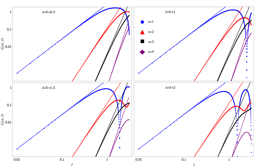
Figure 1: Early time behavior of $C(x,t)$ at different distances. The solid curve is the power law and the dotted curved is the data collected for the OTOC. The system size is $L=1200$. Results are shown for quenches to four different values of $\lambda$ starting from the ground state of the model at $\lambda=0$.

For our purposes the derivation sketched above is too restrictive as we are also interested in non-translationally invariant models and our OTOC features more dynamical terms than just the squared anti-commuter. However, the result, Eq. (13) still remains correct even in the presence of non-zero quasi-periodic potential. This can be seen through the use of the Hadamard formula as shown in Riddell and Sørensen (2019).

We study this prediction in the most dynamically rich way possible, by quenching from the half-filled ground-state at $\lambda=0$ to $\lambda=0.5,1,1.5,2$. Our results are shown in Fig.  1. For a detailed discussion of the starting state see Appendix B. The results here do not significantly change if the quench is to the localized phase ($\lambda=1.5,2$), critical ($\lambda=1)$ or extended phase ($\lambda=0.5$). For all strengths of the quasi-periodic potential is a power-law behaviour observed following Eq. (13). This results agree with Riddell and Sørensen (2019) which found that in an Anderson localized model regardless of the strength of the localization, if the OTOC significantly grows, then the polynomial early time growth Eq. (13) is observed to be hold. This follows naturally from the fact that Eq. (13) is independent of the potential strength, the first contributing dynamics to the OTOC are unaffected by the potential term and come solely from the hopping terms. The early time behaviour can therefore be obtained by studying the $\lambda=0$ case.

III.2 Wavefront

In this section we study the wavefront at different potential strengths and address discrepancies from the results shown in Xu and Swingle (2018a); Khemani et al. (2018) and Riddell and Sørensen (2019). Recently, the universal form was claimed to be confirmed in the XX spin chain, contradictory to earlier claims Bao and Zhang (2019). Here we discuss these seemingly contradictory claims. The universal wave form predicted for the out of time ordered correlator in free theories by means of a standard saddle point approximation scheme is given by Eq. (5) in terms of the Lyapunov exponent, $\lambda_{L}$ and the Butterfly velocity, $v_{B}$. Often this form is applied at surprisingly early times Xu et al. (2019) where $-50<\log(C)<-10$. For the AA model with $\lambda=0$, corresponding to free fermions, we expect the $v_{B}=J$ as the maximal group velocity, and $p=\frac{1}{2}$. The universal form, Eq. (5), cannot be re-expressed in a form equivalent to the ’Gaussian’ form characterized by two spatial and disorder dependent functions $a(x,\lambda)$, $b(x,\lambda)$ proposed in Ref. Riddell and Sørensen, 2019, for times surrounding $x=v_{B}t$, for a fixed $x=x_{0}$:

$$C(x=x_{0},t)\sim e^{-a(x,\lambda)\left(\frac{t^{2}}{2}-\frac{xt}{v_{B}}\right)+b(x,\lambda)t}.$$ (14)

We can rewrite Eq. 14 as,

$$C(x=x_{0},t)\sim e^{-m(x,\lambda)\left(t-\frac{x}{v_{B}}\right)^{2}+b(x,\lambda)t},$$ (15)

where $m(x,\lambda)=a(x,\lambda)/2$.

We expect that the discrepancy is most likely due the existence two unique time regimes that are close together. To eliminate noise in our OTOC we drop all of the dynamical terms except the squared anti-commutator. which is equivalent to instead studying the OTOC,

$$C(x,t)={\rm tr}\left(\{\hat{f}_{m}^{\dagger}(t),\hat{f}_{n}\}\{\hat{f}_{m}(t),\hat{f}_{n}^{\dagger}\}\right)\equiv|a_{m,n}(t)|^{2}.$$ (16)

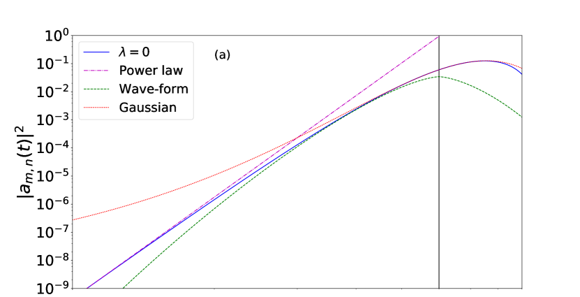
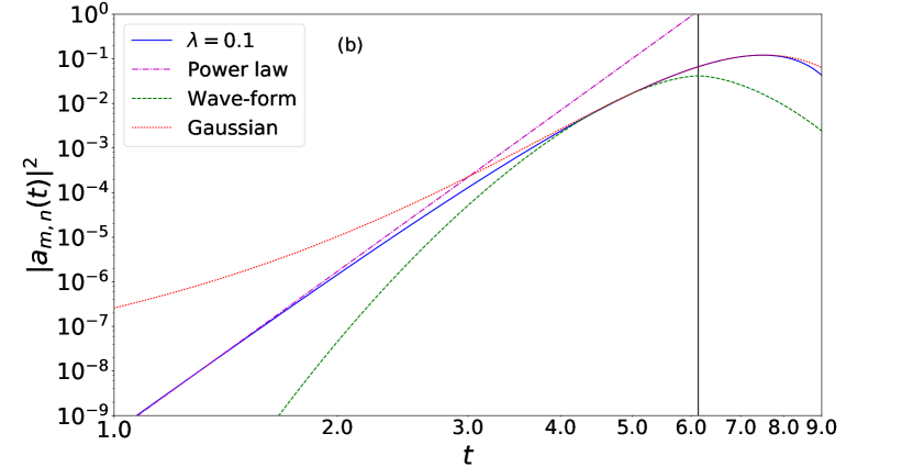
Figure 2: $|a_{m,n}(t)|^{2}$ for $\lambda=0$ (a) and $\lambda=0.1$ (b) plotted with the fitting functions of the early time form, Eq. (13), the proposed universal wave form, Eq. (5) and the Gaussian form, Eq. (15). Results are for a fixed $x=6$ with $L=1600$ and $\lambda=0$. The vertical solid line in both panels corresponds the arrival of the classical wave front at $t=x/v_{B}$ using the fitted $v_{B}$.

To further facilitate the analysis we include a phase, $\phi$, in the potential $\lambda\cos(2\pi\sigma j+\phi)$ and smooth our data by averaging over $\phi$. Our results are shown in Fig. 2 where we follow an analysis similar to Sahu et al. (2018). By varying both time and space we fit the OTOC for $\lambda=0$ in the region such that $\log\left(|a_{m,n}|^{2}\right)\in[-10,-6]$. With this fit we find $v_{B}=0.9950\pm 0.0002$, $p=0.50\pm 0.08$ and $\lambda_{L}=1.78\pm 0.03$ for the universal form, Eq. (5). Where the errors reported are one standard deviation of the parameter estimate. These values are in close agreement with the expected values of $v_{B}=1$ and $p=\frac{1}{2}$. Similarly we investigated the $\lambda=0.1$ case for $\log\left(|a_{m,n}|^{2}\right)\in[-12,-8]$ and found $v_{B}=0.9783\pm 0.0003$, $p=0.647\pm 0.03$ and $\lambda_{L}=2.153\pm 0.09$ for the universal form, Eq. (5). However, these fits correspond to times that significantly precede the classical wavefront. For larger values of the potential strength, $\lambda$, we have found it more difficult to obtain good fits to the universal form, Eq. (5).

At later times the OTOC enters a dynamical regime where the Gaussian form of Eq. 15 is valid. Fixing $x=6$ and using the $v_{B}$ found for the universal form we find that for $\lambda=0$ $m(x,\lambda)=0.3027\pm 0.0001$ and $b(x,\lambda)=0.9470\pm 0.0001$. For $\lambda=0.1$ we find $m(x,\lambda)=0.3052\pm 0.0001$ and $b(x,\lambda)=0.8597\pm 0.0002$.

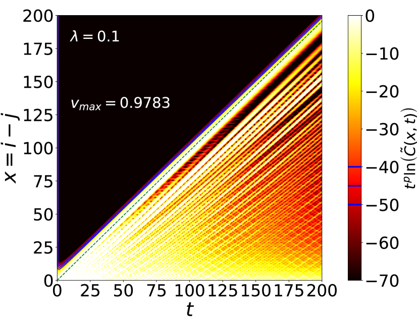
Figure 3: Density plot of $t^{p}\log(\tilde{C})$, with $\tilde{C}$ an appropriately normalized OTOC from Eqn. 16 and $p=0.6470$. Results are shown for $\lambda=0.1$ and $L=1600$. Contour lines are plotted as solid blue lines. The dashed green line indicates $x=v_{B}t$ with $v_{b}=0.9783$ which appear closely parallel to the contour lines.

To further illustrate the universal form, Eq. (5), we show in Fig. 3 results for the entire $C(x,t)$ over a large range of $x$ and $t$ for $\lambda=0.1$. As above we have smoothened the data over the phase $\phi$. We first appropriately normalize $C$ to obtain $\tilde{C}$ and then plot $t^{p}\log(\tilde{C})$ using the fitted $p=0.6470$. We then expect that contour lines should be straight lines defined by $x=v_{b}t$. This is clearly observed in Fig. 3 although we note that it is only contour lines for extremely small values of $t^{p}\log(\tilde{C})$ (of the order of $-40$ to $-50$) that are completely parallel to the determined $v_{B}t$. Although the universal form of Eq. 5 seems to work well, it is only applicable at times $t\ll\frac{x}{v_{B}}$.

Let us return to the Gaussian form of Eq. 15, expected to be valid close to $x=v_{B}t$. We consider the behaviour of the functions $m(x,\lambda)$ and $b(x,\lambda)$ by varying $x$ and fixing $v_{B}$ as the velocities found fitting the universal waveform. These functions appear to asymptotically approach a fixed value in the large $x$ limit.

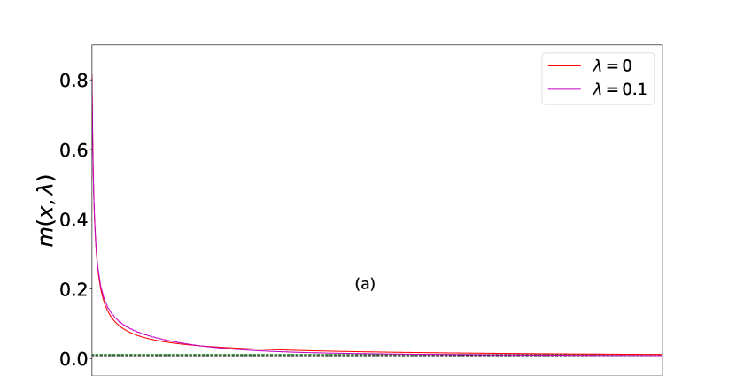
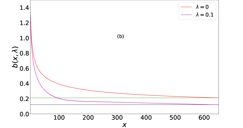
Figure 4: Functions $m(x,\lambda)$ (a) and $b(x,\lambda)$ (b) behaviour for fixed $\lambda$ at different $x$. Results are shown for no $\phi$ averaging and $L=1600$. The dashed green horizontal line corresponds to the observed value of the function at $x=650$ for $\lambda=0$ and the dashed black line to the value for $\lambda=0.1$.

For large $x$ and $\lambda=0$ $m(x,\lambda)\approx 0.01$ and $b(x,\lambda)\approx 0.2$. For $\lambda=0.1$ we see the values $m(x,\lambda)\approx 0.008$ and $b(x,\lambda)\approx 0.1$. This result is shown in Fig. 4. Errors on this parameters are on the order of $10^{-4}$ or smaller. This means that taking large values of distance between the two observables $\hat{A}$ and $\hat{B}$, we may write,

$$C(x,t)\sim e^{-m(t-\frac{x}{v_{B}})^{2}}e^{bt},$$ (17)

where $m$ and $b$ are positive constants. Intuitively this corresponds to a Gaussian wave travelling at velocity $v_{B}$, augmented by $e^{bt}$. This form is expected to be valid on the interval surrounding the passage of classical information around $x=v_{B}t$. Hence, this form for works rather close to $x=v_{B}t$. It seems likely that in interacting systems this might be apparent for much smaller values of $x$.

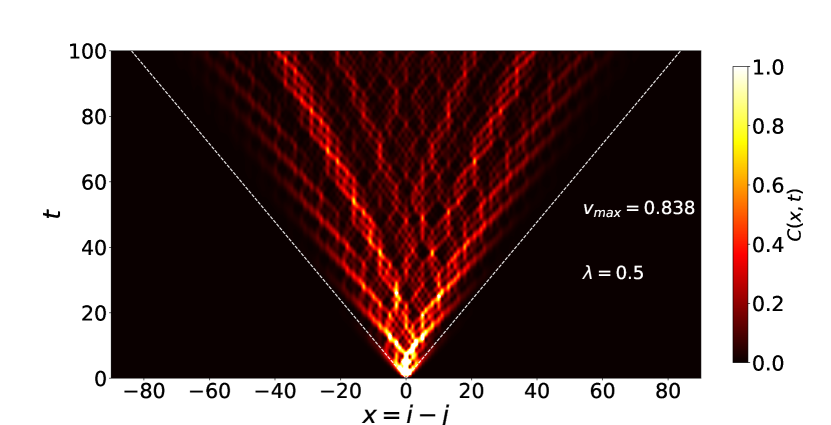
Figure 5: Wavefront spreading in both $x$ and $t$ for $\lambda=0.5$, the center being taken as $\frac{L}{2}$. System size $L=1200$.

If we instead of using the OTOC defined from the anti-commutator, Eq. (16), use the full $C(x,t)$ with a thermal average where we fixed the inverse temperature $\beta=1$ we find typical results as shown in Fig. 5 for $\lambda=0.5$. In this case, as is this case for the remainder of our results we do not smoothen the data using the phase $\phi$. From Fig. 5 we see that the velocity predicted from the universal fit, Eq. (5), of $v_{B}=0.838$ seems to be a good fit for predicting the spread of classical information. For larger values of $\lambda$ we have not found it possible to use the universal form Eq. (16) in contrast to recent results by Xu et al Xu et al. (2019). A possible explanation for this is that Xu et al  Xu et al. (2019) study the behaviour of the OTOC in a thermal state at infinite temperature in an interacting model, a somewhat different setting.

III.3 Late time

It is also interesting to investigate the late time dynamics of the OTOC. In prior studies it was pointed out that a $C(x,t)\sim\frac{1}{t}$ behaviour was expected in late time Bao and Zhang (2019); Lin and Motrunich (2018). These results however are for disorder-free models and do not in general hold for our discussion. So instead we look to analytically show that these OTOCs indeed go to an equilibrium value in the late time regime in the extended phase, regardless of strength of the quasi-periodic potential. To bound this behaviour and prove equilibration we again focus on studying the OTOC defined in terms of the squared anti-commutator, Eq. (16). From Eq. (45) this can be written as:

$$C(x,t) = {\rm tr}\left(\{\hat{f}_{m}^{\dagger}(t),\hat{f}_{n}\}\{\hat{f}_{m}(t),\hat{f}_{n}^{\dagger}\}\right)\equiv\left|a_{m,n}(t)\right|^{2}$$ (18)

$$= \sum_{k,l}A_{m,k}A_{n,k}A_{m,l}A_{n,l}e^{i\left(\epsilon_{k}-\epsilon_{l}\right)t}.$$

The infinite time average is defined as,

$$\left|\omega_{m,n}\right|^{2}=\lim_{T\to\infty}\frac{1}{T}\int_{0}^{T}|a_{m,n}|^{2}dt,$$ (19)

using the fact that $\epsilon_{k}=\epsilon_{l}\Leftrightarrow k=l$,

$$\left|\omega_{m,n}\right|^{2}=\sum_{k}A_{m,k}^{2}A_{n,k}^{2}.$$ (20)

From Eq. (20) we can come to the intuitive conclusion that when the system is extended, in the thermodynamic limit $L\to\infty$, we expect the infinite time average to go to zero. The argument for this is as follows. In the extended phase, the values of $A_{m,k}$ will go like $A_{m,k}\sim\frac{1}{\sqrt{L}}$. Which leads to,

$$\left|\omega_{m,n}\right|^{2}\sim\frac{1}{L},$$ (21)

approaching zero in the thermodynamic limit. This is opposed to the localized phase where we expect, $A_{m,k}\sim e^{-|k-m|/\xi}$, with $\xi$ the localization length and $k=1,\dots L$ Abdul-Rahman et al. (2017) (see lemma 8.1). This makes the infinite time average go like,

$$|w_{m,n}|^{2}\sim\max_{k}e^{-(|k-m|+|k-n|)/\xi}.$$ (22)

Hence, the infinite time average of the OTOC is in this case non-zero within a distance of the order of the localization length.

Next we focus on bounding the relaxation process in time, following Malabarba et al. (2014); García-Pintos et al. (2017); Álvaro M. Alhambra et al. (2019). To study the relaxation we define the positive function,

$$g_{m,n}(t)=\left|\left|a_{m,n}(t)\right|^{2}-\left|\omega_{m,n}\right|^{2}\right|^{2}.$$ (23)

Eq. (23) can be interpreted as the distance the OTOC is from its late time value, assuming such a value exists. To be precise we will work with the time average of the function,

$$\langle g_{m,n}(t)\rangle_{T}=\frac{1}{T}\int_{0}^{T}\left|\sum_{k\neq l}A_{m,k}A_{n,k}A_{m,l}A_{n,l}e^{i\left(\epsilon_{k}-\epsilon_{l}\right)t}\right|^{2}dt,$$ (24)

to make notation easier let $\alpha=(k,l)$ and,

$$v_{\alpha}=A_{m,k}A_{n,k}A_{m,l}A_{n,l},\enspace G_{\alpha}=\epsilon_{k}-\epsilon_{l}.$$ (25)

This allows us to instead write the expression as,

$$\langle g_{m,n}(t)\rangle_{T}=\frac{1}{T}\int_{0}^{T}\sum_{\alpha,\beta}v_{\alpha}v_{\beta}e^{i\left(G_{\alpha}-G_{\beta}\right)t}dt,$$ (26)

We make use of the triangle inequality to make all elements of the sum positive, and then normalize, defining, $Q=\sum_{\alpha}|v_{\alpha}|$,

$$\langle g_{m,n}(t)\rangle_{T}\leq Q^{2}\frac{1}{T}\int_{0}^{T}\sum_{\alpha,\beta}p_{\alpha}p_{\beta}e^{i\left(G_{\alpha}-G_{\beta}\right)t}dt.$$ (27)

It is important to consider how big $Q$ might be. Trivially, $Q\leq\sum_{\alpha}\max_{\alpha}|v_{\alpha}|$. Since this sum over $\alpha$ is quadratic in $L$ and restricting ourselves to the extended regime, Eq. (25) gives, $\max_{\alpha}|v_{\alpha}|\sim\frac{1}{L^{2}}$, it then follows that $Q=O(1)$.

We now introduce the function,

$$\xi_{p}(x)=\max_{\beta}\sum_{\alpha:G_{\beta}\in[G_{\beta},G_{\beta}+x]}p_{\alpha}.$$ (28)

In Appendix D we show that the time average can be bounded using a Gaussian profile, giving,

$$\langle g_{m,n}(t)\rangle_{T}\leq\kappa\pi Q^{2}\xi_{p}\left(\frac{1}{T}\right),$$ (29)

where $\kappa\approx 2.8637$. To further bound this we introduce the two functions,

$$a(\epsilon)=\frac{\xi_{p}(\epsilon)}{\epsilon}\sigma_{G},\enspace\delta(\epsilon)=\xi_{p}(\epsilon),$$ (30)

where $\sigma_{G}=\sqrt{\sum_{\alpha}p_{\alpha}G_{\alpha}^{2}-\left(p_{\alpha}G_{\alpha}\right)^{2}}$ is the standard deviation of our distribution of frequencies. From here on we assume $a(\epsilon)$ and $\delta(\epsilon)$ are implicitly dependent on $m,n$. It can be shown that (proposition 5 of  García-Pintos et al. (2017)):

$$\xi_{p}(x)\leq\frac{a(\epsilon)}{\sigma_{G}}x+\delta(\epsilon).$$ (31)

Using Eq. (31) we can rewrite Eq. 29 as:

$$\langle g_{m,n}(t)\rangle_{T}\leq\kappa\pi Q^{2}\left(\frac{a(\epsilon)}{\sigma_{G}T}+\delta(\epsilon)\right).$$ (32)

Eq. 32 allows us to upper bound the time scale at which the OTOC equilibrates as $T_{eq}=\frac{\kappa\pi a(\epsilon)Q^{2}}{\sigma_{G}}$.

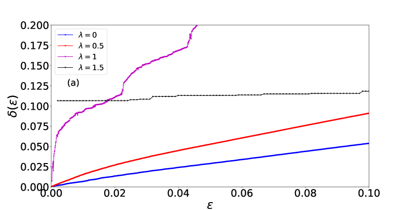
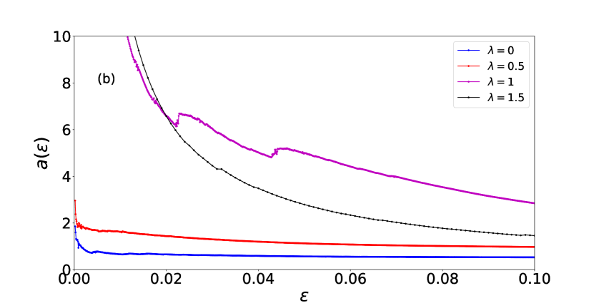
Figure 6: Numerical example of $\delta(\epsilon)$ (panel (a)) and $a(\epsilon)$ (panel (b)) at different system sizes and potential strength for $m=\frac{L}{2},n=\frac{L}{2}+6$, for $L=800$.

Now all that is left is to numerically show that $\delta(\epsilon)$ is quite small. In Fig. 6 we show our results for $a(\epsilon)$ and $\delta(\epsilon)$ at different system sizes and potential strength. From these results we can conclude that the bound performs poorly in the localized regime, and at the critical point of the model, while in the extended regime the bound appears to perform quite well. For the extended regime it appears we may pick an $a(\epsilon)\sim O(1)$ while picking $\delta(\epsilon)\approx 0$, meaning in these cases we expect the OTOC to equilibrate to its infinite time average.

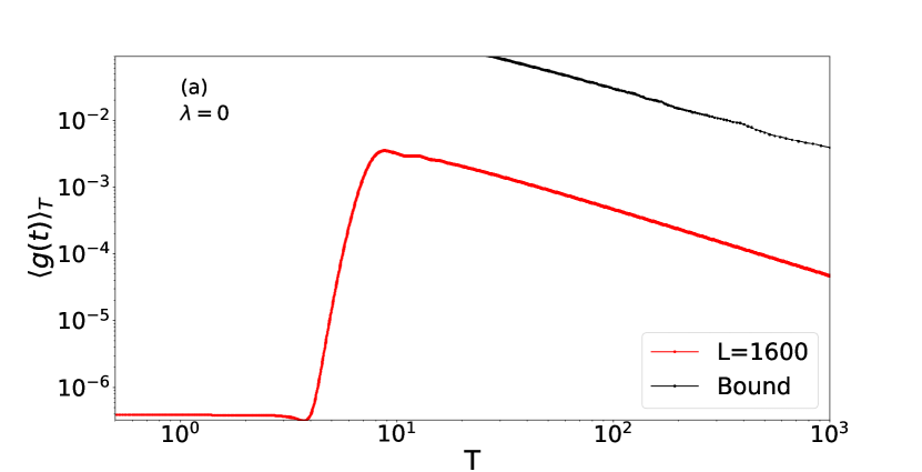
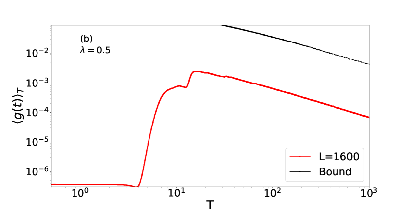
Figure 7: Bound from Eq. (29) for potential strengths $\lambda=0$ (panel (a)) and $\lambda=0.5$ (panel (b)). Both results were computed with $L=1600$ and used $m=\frac{L}{2},n=\frac{L}{2}+6$, $L=1600$.

Next we illustrate the bound, Eq. (29), by numerically evaluating $\langle g_{m,n}(t)\rangle_{T}$ and $\xi(\frac{1}{T})$. Our results are shown in Fig. 7 where we see that, as predicted, the time average defined in Eq. (24) is not only upper bounded by Eq. (29), but as the time interval $T$ is increase this upper bound decays to zero in the extended region. Thus, this constitutes equilibration of an OTOC in both a translationally invariant case ($\lambda=0$), and a case with a non-zero quasi-periodic potential ($\lambda=0.5$). This result is expected to hold for $\lambda\in[0,\lambda_{\text{critical}})$ where for the present numerics we have, $\lambda_{\text{critical}}=1$. Furthermore, we stress that this result should be applicable to all quadratic models in their extended phases.

Next we consider relaxation in the infinite time limit $T\to\infty$. Here, the quantity to bound (assuming for simplicity non-degenerate mode gaps, and excluding the localized and critical regimes) is,

$$\lim_{T\to\infty}\langle g_{m,n}(t)\rangle_{T}=\sum_{k\neq l}A_{m,k}^{2}A_{n,k}^{2}A_{m,l}^{2}A_{n,l}^{2}.$$ (33)

From Eq. (33), using $A_{m,k}^{2}\sim\frac{1}{L}$, we see that with four such terms and only a quadratic summation over these terms $\lim_{T\to\infty}\langle g_{m,n}(t)\rangle_{T}$ must go to zero in the extended region. To put this into more rigorous terms we may define the constant $c=L\max_{k}\{A_{m,k}^{2},A_{n,k}^{2}\}$ such that,

$$\lim_{T\to\infty}\langle g_{m,n}(t)\rangle_{T}\leq c^{4}\sum_{k\neq l}\frac{1}{L^{4}}\leq\frac{c^{4}}{L^{2}},$$ (34)

where $c$ is independent of system size due to the terms $\sqrt{L}A_{m,k}=O(1)$.

IV Momentum OTOCs

In this section we study the out of time order correlators with momentum number operators, and set,

$$\hat{A}(t)=2\hat{\eta}_{\pi}^{\dagger}(t)\hat{\eta}_{\pi}(t)-1\enspace\text{,}\enspace\hat{B}=2\hat{\eta}_{\pi}^{\dagger}\hat{\eta}_{\pi}-1.$$ (35)

The OTOC then corresponds to the $k=\pi$ momentum operator commuting with itself in time. We make this choice since, although two momenta $k$ and $l$ could be neighbours in momentum space, this distance isn’t physical and no wave front can be defined. The choice of $k=\pi$ is arbitrary but sits in the ”middle” of momentum space. To distinguish our results from the previous sections, where real space OTOCs were discussed, we denote the OTOC $C_{p}(t)$ in this section, suppressing the $x$ dependence of $C$. The system size throughout this section is set to $L=400$, no significant differences were observed for systems sizes up to $L=1200$.

IV.1 Quenching

The momentum OTOCs are studied by quenching from the ground state of the initial Hamiltonian. This is done in a manner identically to section III. First we consider quenching from an initial potential strength$\lambda_{i}=0$.

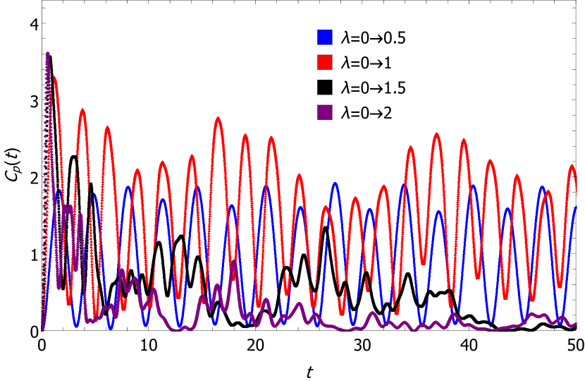
Figure 8: $C_{p}(t)$ plotted from the dynamics of a ground state of a Hamiltonian characterized by $\lambda_{i}=0$ to various final Hamiltonians. This corresponds to quenching from the extended region into the critical point at $\lambda=1$, extended phase $\lambda=0.5$ and two examples of the localized phase $\lambda=1.5,2$. Results are for $L=400$.

Fig. 8 shows $C_{p}(t)$ quenched from the ground state of the Hamiltonian with $\lambda_{i}=0$ then quenched and time evolved with new values of $\lambda_{f}=0.5,1,1.5,2$. Interestingly, the OTOCs all attain a maximum, at quite early times $t<4$, and then display a slow decay from the largest value. The localized phase dynamics for potential strengths of$\lambda_{f}=1.5,2$ clearly show that the momentum OTOC eventually decay to zero, and oscillate near it. The extended phase oscillates away from zero, but does not appear to reach it. At the critical point, $\lambda_{c}=1$ pronounced oscillations is observed exceeding all other $\lambda_{f}$. The extended state is characterized by oscillations around a fixed non-zero with this value rising with $\lambda_{f}$ as it approaches $\lambda_{f}=\lambda_{c}$.

As can be clearly seen from Fig. 8, the dynamics are quite complex and it is desirable to understand the asymptotic behaviour at the wavefront, which we can tentatively define as the first occurrence where $C(t)$ decreases. Since the momentum OTOCs are highly non-local in real space the proposed universal form, Eq. (5), is not directly applicable and we therefore consider an ad-hoc form

$$f(x)=C\exp(at+b/t+c/t^{2}+d/t^{3}).$$ (36)

Figure 9: $\log C_{p}(t)$ plotted from the dynamics of a ground state of a Hamiltonian characterized by $\lambda_{i}=0$ to various final Hamiltonians characterized by different $\lambda_{f}$. This data is then fitted to the function, $f(t)=C\exp(at+b/t+c/t^{2}+d/t^{3})$, which is then graphed. Results are for $L=400$

Results by fitting to the form, Eq. (36) are shown in Fig. 9 for several different values of $\lambda_{f}$. Extremely good fits are obtained and we have verified that adding more terms does not significantly improve the fits.

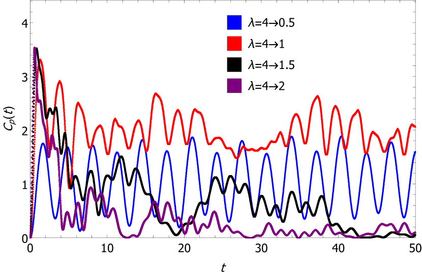
Figure 10: $C_{p}(t)$ plotted from the dynamics of a ground state of a Hamiltonian characterized by $\lambda=4$ to various final Hamiltonians. This corresponds to quenching from the extended region into the critical point at $\lambda=1$, extended phase $\lambda=0.5$ and two examples of the localized phase $\lambda=1.5,2$. Results are for $L=400$.

Next we consider a different quench where we instead start from the localized phase with $\lambda_{i}=4$ and evolve with the four different $\lambda_{f}=0.5,1,1.5,2$. Our results for this case are shown in Fig. 10. The oscillations in this case comparably to quecnhing from $\lambda_{i}=0$ shown in Fig. 8. However, their quasi-periodicity is much smaller and less chaotic. Both examples, $\lambda_{i}=0,4$, are characterized by the same oscillations that appear to never dissipate. However, the wavefront for $\lambda_{i}=4$ is near identical to the one shown in Fig. 9 for $\lambda_{i}=0$. The same function, Eq. (36), used to fit the results for $\lambda_{i}=0$ can be used to characterize the wavefront for $\lambda_{i}=4$ producing extremely high quality fits almost indistinguishable from the fits shown in Fig. 9. Thus we conclude that the initial rise of the OTOC goes like Eq. (36) in both quench scenarios. The form given in Eq. (46) was also observed to hold for momentum OTOCs defined in a thermal states, as well as for initial states in the form of a product state:

$$|\psi\rangle=\prod_{l\in\mathbb{S}}\hat{f}_{l}^{\dagger}|0\rangle.$$ (37)

where $\mathbb{S}=\{l\in\mathbb{N}:l\mod 2=0\}$. This then allows us to conclude that this form of the wavefront for momentum OTOCs is rather generic, and doesn’t depend on initial conditions.

V Conclusion

The AA model with a quasi-periodic potential represents a unique opportunity to investigate quantum information dynamics in the presence of a phase transition between an extended localized phase using exact numerics. Here we have explicitly demonstrated equilibration of the real-space OTOCs to zero in the extended phase of the model, a result that generalizes to any model with quadratic interactions in an extended regime. The early time behavior of the real-space OTOCs are largely independent of the strength of the quasi-periodic potential and follow a simple power-law with position dependent exponent even in the localized phase. The regime close to the classical wavefront, $x=v_{B}t$, has been shown to propagate as a Gaussian (Eq. 15) with distance dependent parameters which converge to constants in the large distance limit, signifying a fifth time regime of interest for the OTOC. At earlier times $t\ll\frac{x}{v_{B}}$ it is possible to apply the universal waveform Eq. 5 which is often applied to thermal OTOCs at infinite temperature. The spreading of information in momentum space as obtained from analyzing momentum space OTOCs is significantly more complex and a complete understanding is currently lacking. Here we propose an ad-hoc form for the early time behaviour of the momentum OTOCs that seem to work exceedingly well.

VI Acknowledgements

J.R would like to thank Álvaro M. Alhambra, Luis Pedro García-Pintos and Shenglong Xu for helpful discussions. This research was supported by NSERC and enabled in part by support provided by (SHARCNET) (www.sharcnet.ca) and Compute/Calcul Canada (www.computecanada.ca).

Appendix A Time evolution

In this appendix entry we review time evolution of free fermions and present out the numerical method required to carry out of quench protocol. For more detailed treatments of the time evolution of free fermions see Riddell and Sørensen (2019),Perarnau-Llobet et al. (2016). We are given in general a Hamiltonian written in the form,

$$\hat{H}=\sum_{i,j}M_{i,j}\hat{f}_{i}^{\dagger}\hat{f}_{j}.$$ (38)

Where we assume $M$ is real symmetric and thus can be diagonilized with a real orthogonal matrix $A$ such that $M=ADA^{\dagger}$. This solves the model, and we recover new fermionic operators and a diagonal Hamiltonian,

$$\hat{H}=\sum_{k}\epsilon_{k}\hat{d}_{k}^{\dagger}\hat{d}_{k},$$ (39)

where we refer to $\epsilon_{k}$ as energy eigenmodes which are the entries of the diagonal matrix and the corresponding space, eigenmode space (normal modes is also regularly used). Since the states we are interested in are Gaussian (product states, thermal states, ground states), we can completely deduce all statistics of the model with the occupation matrix. Defining arbitrary fermionic operators as $\hat{b}_{k}^{\dagger}$, $\hat{b}_{l}$ we define the matrix in $b$ space as,

$$\Lambda_{k,l}^{(b)}=\langle\hat{b}_{k}^{\dagger}\hat{b}_{l}\rangle.$$ (40)

Where the superscript denotes the space we are describing. In this document we refer to real space with $f$, eigenmode space with $d$ and momentum space with $p$ superscripts. Time evolving individual eigenmodes is easily deduced from Eq. (39),

$$\hat{d}_{k}(t)=e^{-i\epsilon_{k}t}\hat{d}_{k}.$$ (41)

For the creation operators simply take the Hermitian adjoint. As seen in Eq. (84), we are interested in time evolving one or two operators in the expectation value. Thus we see that evolving the whole matrix in real space we get,

$$\Lambda^{(f)}(t,t)=Ae^{iDt}\Lambda^{(d)}e^{-iDt}A^{T}.$$ (42)

Where the double time arguments signify we are time evolving both the creation and annihilation part. Similarly the out of time correlations in real space can be calculated from,

$$\Lambda^{(f)}(t,0)=Ae^{iDt}\Lambda^{(d)}A^{T}\enspace\text{,}\enspace\Lambda^{(f)}(0,t)=A\Lambda^{(d)}e^{-iDt}A^{T}.$$ (43)

From here we can calculate the correlation functions of the momentum operators given by,

$$\eta_{k}:=\frac{1}{\sqrt{L}}\sum_{j}e^{ikj}\hat{f}_{j},$$

$$\eta_{k}^{\dagger}:=\frac{1}{\sqrt{L}}\sum_{j}e^{-ikj}\hat{f}_{j}^{\dagger}.$$

Then the correlations in momentum space are given by,

$$\Lambda^{(p)}_{k,l}=\sum_{m,n}e^{-i(mk-nl)}\Lambda_{m,n}^{(f)}.$$ (44)

The time evolution is then found by time evolving $\Lambda_{m,n}^{(f)}$ in the desired way. Now all we need to describe is the out of time anti-commutation relations. For the real space operators,

$$\{\hat{f}_{m}^{\dagger}(t),\hat{f}_{n}\}=\sum_{k}{A}_{m,k}A_{n,k}e^{i\epsilon_{k}t}=a_{m,n}(t),$$ (45)

simply taking the conjugate recovers the relationship where $\hat{f}_{n}$ is time evolved. We also have, $\{\hat{f}_{m}(t),\hat{f}_{n}\}=\{\hat{f}_{m}^{\dagger}(t),\hat{f}_{n}^{\dagger}\}=0$. For the momentum operators ,

$$\{\eta_{k}^{\dagger}(t),\eta_{p}\}=\frac{1}{L}\sum_{m,n}e^{-i(km-pn)}\left(\hat{f}_{m}^{\dagger}(t)\hat{f}_{n}+\hat{f}_{n}\hat{f}_{m}^{\dagger}(t)\right)=\frac{1}{L}\sum_{m,n}e^{-i(km-pn)}a_{m,n}(t)=u_{k,p}(t).$$ (46)

Eq. (46) is simply a discrete Fourier transform of Eq. (45). With these pieces we can now calculate the necessary correlators and out of time anti-commutators for the OTOC.

Appendix B Quench protocol

We now turn to a discussion of the quench protocol. We define two Hamiltonians written identically to the one written in Eq. (38), with $\hat{H}^{(1)}$ and $\hat{H}^{(2)}$. We first prepare the ground state of $\hat{H}^{(1)}$ by diagonalizing $M^{(1)}$, let $\epsilon_{k}^{(1)}$ be its eigenvalues, and preparing the eigenmode state with,

$$\Lambda_{k,l}^{(d,1)}=\langle\hat{d}_{k}^{\dagger}\hat{d}_{l}\rangle=\left\{\begin{array}[]{cl}1&k=l\land\epsilon_{k}^{(1)}<0\\ 0&\text{otherwise}.\end{array}\right.$$ (47)

Note that in some cases we might have $\epsilon_{k}^{(1)}=0$ for some value of $k$, making the ground state degenerate. We then choose to construct the ground state which only has negative eigenmodes occupied and neglect the zero. We then transform the occupation matrix to real space,

$$\Lambda^{(f)}(0,0)=A^{(1)T}\Lambda^{(d,1)}A^{(1)}.$$ (48)

This gives us the initial correlation functions. Next we imagine suddenly changing the Hamiltonian to $\hat{H}^{(2)}$. We can now find this states representation in the eigenmode of the new Hamiltonian by using its orthogonal transform, $\Lambda^{(d,2)}=A^{(2)T}\Lambda^{(f)}A^{(2)}$ Thus the time evolution we are interested in is written as,

$$\Lambda^{(f)}(t,t)=A^{(2)}e^{iD^{(2)}t}\Lambda^{(d,2)}e^{-iD^{(2)}t}A^{(2)T},$$ (49)

$$\Lambda^{(f)}(t,0)=A^{(2)}e^{iD^{(2)}t}\Lambda^{(d,2)}A^{(2)T},$$ (50)

$$\Lambda^{(f)}(0,t)=A^{(2)}\Lambda^{(d,2)}e^{-iD^{(2)}t}A^{(2)T}.$$ (51)

This representation allows us to compute statistic we could be interested in for a Gaussian state.

Appendix C Calculating the OTOCs

Here we present the calculation of the OTOCs in terms of second moments. In all three cases we are interested in; product states, thermal states and ground states, are Gaussian. Thus we can use Wick’s theorem to calculate the OTOC. This is done similarly to Riddell and Sørensen (2019). Here we present the derivation for $F_{b}(x,t)$ for arbitrary lattice points and fermionic operators. Consider arbitrary fermionic operators $\hat{b}_{i}$ such that $\{\hat{b}_{k},\hat{b}_{l}\}=\{\hat{b}_{k}^{\dagger},\hat{b}_{l}^{\dagger}\}=0$, $\{\hat{b}_{l}^{\dagger},\hat{b}_{k}\}=\delta_{l,k}$ and $a_{m,n}(t)=\{\hat{b}_{m}^{\dagger}(t),\hat{b}_{n}\}$, where we assume $\{\hat{b}_{m}(t),\hat{b}_{n}\}=\{\hat{b}_{m}^{\dagger}(t),\hat{b}_{n}^{\dagger}\}=0$. Then we are interested in the real part of the function,

$$F_{b}(x,t)=\langle\left(\hat{b}_{i}^{\dagger}(t)\hat{b}_{i}(t)-\frac{1}{2}\right)\left(\hat{b}_{j}^{\dagger}\hat{b}_{j}-\frac{1}{2}\right)\left(\hat{b}_{i}^{\dagger}(t)\hat{b}_{i}(t)-\frac{1}{2}\right)\left(\hat{b}_{j}^{\dagger}\hat{b}_{j}-\frac{1}{2}\right)\rangle.$$ (52)

Adopting the notation $\hat{n}_{i}=\hat{b}_{i}^{\dagger}\hat{b}_{i}$ and using $\hat{n}_{i}(t)^{2}=n_{i}(t)$ we can write,

$$F(t)=16\langle\hat{n}_{i}(t)\hat{n}_{j}\hat{n}_{i}(t)\hat{n}_{j}-\frac{1}{2}(\hat{n}_{i}(t)\hat{n}_{j}\hat{n}_{i}(t)+\hat{n}_{j}\hat{n}_{i}(t)\hat{n}_{j})+\frac{1}{4}(\hat{n}_{j}\hat{n}_{i}(t)-\hat{n}_{i}(t)\hat{n}_{j})+\frac{1}{16}\rangle.$$ (53)

Here we present the derivation for the thermal state, but since all states considered are Gaussian the end result will be equivalent. Throughout the derivation we abuse the fact that $\hat{b}_{i}^{2}=\left(\hat{b}_{i}^{\dagger}\right)^{2}=0$, the out of time anti-commutation rules, and assuming that each $\hat{b}_{k}$ is a linear combination of $\hat{d}_{l}$ terms only. Now we can focus on treating each term based on our initial conditions as before. Let us deal with each term of $F(t)$ individually. First consider the fourth order correlations,

$$\langle\hat{n}_{j}\hat{n}_{i}(t)-\hat{n}_{i}(t)\hat{n}_{j}\rangle_{\beta}.$$ (54)

Let us derive a rule to contract these fourth moments. Consider,

$$\langle\hat{n}_{i}(t)\hat{n}_{j}\rangle_{\beta}=\langle\hat{b}_{i}^{\dagger}(t)\hat{b}_{i}(t)\hat{b}_{j}^{\dagger}\hat{b}_{j}\rangle_{\beta}=\sum_{m,n,k,l}A_{i,k}A_{i,l}A_{j,m}A_{j,n}e^{i(\epsilon_{k}-\epsilon_{l}t)}\langle\hat{d}_{k}^{\dagger}\hat{d}_{l}\hat{d}_{m}^{\dagger}\hat{d}_{n}\rangle_{\beta}.$$ (55)

Using the fact that,

$$\Lambda_{k,l}^{d,\beta}=\langle\hat{d}_{k}^{\dagger}\hat{d}_{l}\rangle_{\beta}=\left\{\begin{array}[]{cl}\frac{1}{1+e^{\beta\epsilon_{k}}}&k=l,\\ 0&\text{otherwise}.\end{array}\right.$$ (56)

$${\rm tr}\left(\hat{d}_{k}^{\dagger}\hat{d}_{l}\hat{d}_{m}^{\dagger}\hat{d}_{n}\rho_{\beta}\right)=\delta_{k,l}{\rm tr}(\hat{d}_{m}^{\dagger}\hat{d}_{n}\rho_{\beta})+\delta_{k,n}{\rm tr}(\hat{d}_{l}\hat{d}_{m}^{\dagger}\rho_{\beta})-{\rm tr}(\hat{d}_{l}\hat{d}_{m}^{\dagger}\hat{d}_{n}\hat{d}_{k}^{\dagger}\rho_{\beta}).$$ (57)

Using $e^{-\beta\epsilon_{k}\hat{n}_{k}}\hat{d}_{k}^{\dagger}=e^{-\beta\epsilon_{k}}\hat{d}_{k}^{\dagger}e^{-\beta\epsilon_{k}\hat{n}_{k}}$ we get,

$$(1+e^{\beta\epsilon_{k}}){\rm tr}\left(\hat{d}_{k}^{\dagger}\hat{d}_{l}\hat{d}_{m}^{\dagger}\hat{d}_{n}\rho_{\beta}\right)=\delta_{k,l}{\rm tr}(\hat{d}_{m}^{\dagger}\hat{d}_{n}\rho_{\beta})+\delta_{k,n}{\rm tr}(\hat{d}_{l}\hat{d}_{m}^{\dagger}\rho_{\beta}),$$ (58)

$$\implies{\rm tr}\left(\hat{d}_{k}^{\dagger}\hat{d}_{l}\hat{d}_{m}^{\dagger}\hat{d}_{n}\rho_{\beta}\right)=\langle\hat{d}_{k}^{\dagger}\hat{d}_{l}\rangle{\rm tr}(\hat{d}_{m}^{\dagger}\hat{d}_{n}\rho_{\beta})+\langle\hat{d}_{k}^{\dagger}\hat{d}_{n}\rangle{\rm tr}(\hat{d}_{l}\hat{d}_{m}^{\dagger}\rho_{\beta}).$$ (59)

This then gives,

$$\langle\hat{n}_{i}(t)\hat{n}_{j}\rangle_{\beta}=\langle\hat{b}_{i}^{\dagger}(t)\hat{b}_{i}(t)\rangle_{\beta}\langle\hat{b}_{j}^{\dagger}\hat{b}_{j}\rangle_{\beta}+\langle\hat{b}_{i}^{\dagger}(t)\hat{b}_{j}\rangle_{\beta}\langle\hat{b}_{i}(t)\hat{b}_{j}^{\dagger}\rangle_{\beta}.$$ (60)

Similarly,

$$\langle\hat{n}_{j}\hat{n}_{i}(t)\rangle_{\beta}=\langle\hat{b}_{j}^{\dagger}\hat{b}_{j}\rangle_{\beta}\langle\hat{b}_{i}^{\dagger}(t)\hat{b}_{i}(t)\rangle_{\beta}+\langle\hat{b}_{j}^{\dagger}\hat{b}_{i}(t)\rangle_{\beta}\langle\hat{b}_{j}\hat{b}_{i}^{\dagger}(t)\rangle_{\beta}$$ (61)

From here we see that,

$$\langle\hat{n}_{j}\hat{n}_{i}(t)\rangle_{\beta}-\langle\hat{n}_{i}(t)\hat{n}_{j}\rangle_{\beta}=\langle\hat{b}_{j}^{\dagger}\hat{b}_{i}(t)\rangle_{\beta}\langle\hat{b}_{j}\hat{b}_{i}^{\dagger}(t)\rangle_{\beta}-\langle\hat{b}_{i}^{\dagger}(t)\hat{b}_{j}\rangle\langle\hat{b}_{i}(t)\hat{b}_{j}^{\dagger}\rangle_{\beta},$$ (62)

$$=\langle\hat{b}_{j}^{\dagger}\hat{b}_{i}(t)\rangle_{\beta}\left(a_{i,j}(t)-\langle\hat{b}_{i}^{\dagger}(t)\hat{b}_{j}\rangle_{\beta}\right)-\langle\hat{b}_{i}^{\dagger}(t)\hat{b}_{j}\rangle_{\beta}\left(\bar{a}_{i,j}(t)-\langle\hat{b}_{j}^{\dagger}\hat{b}_{i}(t)\rangle_{\beta}\right)=a_{i,j}(t)\langle\hat{b}_{j}^{\dagger}\hat{b}_{i}(t)\rangle_{\beta}-\bar{a}_{i,j}(t)\langle\hat{b}_{i}^{\dagger}(t)\hat{b}_{j}\rangle_{\beta},$$ (63)

this is however a purely imaginary number and therefore does not contribute to the OTOC. Now the sixth order term,

$$\hat{n}_{j}\hat{n}_{i}(t)\hat{n}_{j}=\hat{b}_{j}^{\dagger}\hat{b}_{j}\hat{b}_{i}^{\dagger}(t)\hat{b}_{i}(t)\hat{b}_{j}^{\dagger}\hat{b}_{j},$$ (64)

$$=\hat{b}_{j}^{\dagger}\left(a_{i,j}(t)-\hat{b}_{i}^{\dagger}(t)\hat{b}_{j}\right)\hat{b}_{i}(t)\hat{b}_{j}^{\dagger}\hat{b}_{j},$$ (65)

$$=a_{i,j}(t)\hat{b}_{j}^{\dagger}\hat{b}_{i}(t)\hat{b}_{j}^{\dagger}\hat{b}_{j}-\hat{b}_{j}^{\dagger}\hat{b}_{i}^{\dagger}(t)\hat{b}_{j}\hat{b}_{i}(t)\hat{b}_{j}^{\dagger}\hat{b}_{j},$$ (66)

$$=a_{i,j}\hat{b}_{j}^{\dagger}\left(\bar{a}_{i,j}(t)-\hat{b}_{j}^{\dagger}\hat{b}_{i}(t)\right)\hat{b}_{j}+\hat{b}_{j}^{\dagger}\hat{b}_{i}^{\dagger}(t)\hat{b}_{i}(t)\hat{b}_{j}\hat{b}_{j}^{\dagger}\hat{b}_{j},$$ (67)

$$|a_{i,j}|^{2}\hat{b}_{j}^{\dagger}\hat{b}_{j}+\hat{b}_{j}^{\dagger}\hat{b}_{i}^{\dagger}(t)\hat{b}_{i}(t)\left(1-\hat{b}_{j}^{\dagger}\hat{b}_{j}\right)\hat{b}_{j},$$ (68)

$$=|a_{i,j}|^{2}\hat{b}_{j}^{\dagger}\hat{b}_{j}+\hat{b}_{j}^{\dagger}\hat{b}_{i}^{\dagger}(t)\hat{b}_{i}(t)\hat{b}_{j}.$$ (69)

Then applying the expectation value,

$$|a_{i,j}|^{2}\langle\hat{b}_{i}^{\dagger}(t)\hat{b}_{i}(t)\rangle_{\beta}+\langle\hat{b}_{i}^{\dagger}(t)\hat{b}_{j}^{\dagger}\hat{b}_{j}\hat{b}_{i}(t)\rangle_{\beta},$$ (70)

$$=|a_{i,j}|^{2}\langle\hat{b}_{i}^{\dagger}(t)\hat{b}_{i}(t)\rangle_{\beta}+\sum_{m,n,k,l}A_{i,k}A_{j,l}A_{j,m}A_{i,n}e^{i(\epsilon_{k}-\epsilon_{n}t)}\langle\hat{d}_{k}^{\dagger}\hat{d}_{l}^{\dagger}\hat{d}_{m}\hat{d}_{n}\rangle_{\beta},$$ (71)

$$=|a_{i,j}|^{2}\langle\hat{b}_{i}^{\dagger}(t)\hat{b}_{i}(t)\rangle_{\beta}+\sum_{m,n,k,l}A_{i,k}A_{j,l}A_{j,m}A_{i,n}e^{i(\epsilon_{k}-\epsilon_{n}t)}\left(-\langle\hat{d}_{k}^{\dagger}\hat{d}_{m}\rangle_{\beta}\langle\hat{d}_{l}^{\dagger}\hat{d}_{n}\rangle_{\beta}+\langle\hat{d}_{k}^{\dagger}\hat{d}_{n}\rangle_{\beta}\langle\hat{d}_{l}^{\dagger}\hat{d}_{m}\rangle_{\beta}\right),$$ (72)

$$=|a_{i,j}|^{2}\langle\hat{b}_{i}^{\dagger}(t)\hat{b}_{i}(t)\rangle_{\beta}+\langle\hat{b}_{j}^{\dagger}\hat{b}_{j}\rangle_{\beta}\langle\hat{b}_{i}(t)^{\dagger}\hat{b}_{i}(t)\rangle_{\beta}-\langle\hat{b}_{j}^{\dagger}\hat{b}_{i}(t)\rangle_{\beta}\langle\hat{b}_{i}^{\dagger}(t)\hat{b}_{j}\rangle_{\beta}$$ (73)

Next we look at the other 6th moment,

$$\hat{n}_{i}(t)\hat{n}_{j}\hat{n}_{i}(t)=\hat{b}_{i}^{\dagger}(t)\hat{b}_{i}(t)\hat{b}_{j}^{\dagger}\hat{b}_{j}\hat{b}_{i}^{\dagger}(t)\hat{b}_{i}(t).$$ (74)

The strategy here is identical, and we arrive at,

$$\hat{n}_{i}(t)\hat{n}_{j}\hat{n}_{i}(t)=|a_{i,j}|^{2}\hat{b}_{i}^{\dagger}(t)\hat{b}_{i}(t)+\hat{b}_{i}^{\dagger}(t)\hat{b}_{j}^{\dagger}\hat{b}_{j}\hat{b}_{i}(t).$$ (75)

Applying the thermal expectation value,

$$\langle\hat{n}_{i}(t)\hat{n}_{j}\hat{n}_{i}(t)\rangle_{\beta}=|a_{i,j}|^{2}\langle\hat{b}_{i}^{\dagger}(t)\hat{b}_{i}(t)\rangle_{\beta}+\langle\hat{b}_{i}^{\dagger}(t)\hat{b}_{j}^{\dagger}\hat{b}_{j}\hat{b}_{i}(t)\rangle_{\beta},$$ (76)

$$=|a_{i,j}|^{2}\langle\hat{b}_{i}^{\dagger}(t)\hat{b}_{i}(t)\rangle_{\beta}+\langle\hat{b}_{j}^{\dagger}\hat{b}_{j}\rangle_{\beta}\langle\hat{b}_{i}(t)^{\dagger}\hat{b}_{i}(t)\rangle_{\beta}-\langle\hat{b}_{j}^{\dagger}\hat{b}_{i}(t)\rangle_{\beta}\langle\hat{b}_{i}^{\dagger}(t)\hat{b}_{j}\rangle_{\beta}.$$ (77)

So we finally need the eighth order term which is made easier by knowing the results from the 6th order terms,

$$\hat{n}_{i}(t)\hat{n}_{j}\hat{n}_{i}(t)\hat{n}_{j}=\hat{b}_{i}^{\dagger}(t)\hat{b}_{i}(t)\left(\hat{b}_{j}^{\dagger}\hat{b}_{j}\hat{b}_{i}^{\dagger}(t)\hat{b}_{i}(t)\hat{b}_{j}^{\dagger}\hat{b}_{j}\right),$$ (78)

$$=\hat{b}_{i}^{\dagger}(t)\hat{b}_{i}(t)\left(|a_{i,j}(t)|^{2}\hat{b}_{j}^{\dagger}\hat{b}_{j}+\hat{b}_{j}^{\dagger}\hat{b}_{i}^{\dagger}(t)\hat{b}_{i}(t)\hat{b}_{j}\right),$$ (79)

$$=|a_{i,j}(t)|^{2}\hat{b}_{i}^{\dagger}(t)\hat{b}_{i}(t)\hat{b}_{j}^{\dagger}\hat{b}_{j}+\hat{b}_{i}^{\dagger}(t)\hat{b}_{i}(t)\hat{b}_{j}^{\dagger}\hat{b}_{i}^{\dagger}(t)\hat{b}_{i}(t)\hat{b}_{j},$$ (80)

$$=|a_{i,j}(t)|^{2}\hat{b}_{i}^{\dagger}(t)\hat{b}_{i}(t)\hat{b}_{j}^{\dagger}\hat{b}_{j}+\hat{b}_{j}^{\dagger}\hat{b}_{i}^{\dagger}(t)\hat{b}_{i}(t)\hat{b}_{j}.$$ (81)

Now, taking the thermal expectation value we can use previous results, (the first term is from the fourth moments, and second from the sixth) ,

$$=|a_{i,j}(t)|^{2}(\langle\hat{b}_{i}^{\dagger}(t)\hat{b}_{i}(t)\rangle_{\beta}\langle\hat{b}_{j}^{\dagger}\hat{b}_{j}\rangle_{\beta}+\langle\hat{b}_{i}^{\dagger}(t)\hat{b}_{j}\rangle_{\beta}\langle\hat{b}_{i}(t)\hat{b}_{j}^{\dagger}\rangle_{\beta})+\langle\hat{b}_{i}^{\dagger}(t)\hat{b}_{i}(t)\rangle_{\beta}\langle\hat{b}_{j}^{\dagger}\hat{b}_{j}\rangle_{\beta}-\langle\hat{b}_{i}^{\dagger}(t)\hat{b}_{j}\rangle_{\beta}\langle\hat{b}_{j}^{\dagger}\hat{b}_{i}(t)\rangle_{\beta},$$ (82)

$$=|a_{i,j}(t)|^{2}(\langle\hat{b}_{i}^{\dagger}(t)\hat{b}_{i}(t)\rangle_{\beta}\langle\hat{b}_{j}^{\dagger}\hat{b}_{j}\rangle_{\beta}+\langle\hat{b}_{i}^{\dagger}(t)\hat{b}_{j}\rangle_{\beta}\langle\bar{a}_{i,j}(t)-\hat{b}_{j}^{\dagger}\hat{b}_{i}(t)\rangle_{\beta})+\langle\hat{b}_{i}^{\dagger}(t)\hat{b}_{i}(t)\rangle_{\beta}\langle\hat{b}_{j}^{\dagger}\hat{b}_{j}\rangle_{\beta}-\langle\hat{b}_{i}^{\dagger}(t)\hat{b}_{j}\rangle_{\beta}\langle\hat{b}_{j}^{\dagger}\hat{b}_{i}(t)\rangle_{\beta}$$ (83)

Grouping everything together finally gives us,

$$F_{b}(x,t)=16|a_{i,j}(t)|^{2}\left(\langle\hat{b}_{i}^{\dagger}(t)\hat{b}_{i}(t)\rangle_{\beta}\langle\hat{b}_{j}^{\dagger}\hat{b}_{j}\rangle_{\beta}-\frac{1}{2}\left(\langle\hat{b}_{i}^{\dagger}(t)\hat{b}_{i}(t)\rangle_{\beta}+\langle\hat{b}_{j}^{\dagger}\hat{b}_{j}\rangle_{\beta}\right)+\bar{a}_{i,j}(t)\langle\hat{b}_{i}^{\dagger}(t)\hat{b}_{j}\rangle_{\beta}-\langle\hat{b}_{i}^{\dagger}(t)\hat{b}_{j}\rangle_{\beta}\langle\hat{b}_{j}^{\dagger}\hat{b}_{i}(t)\rangle_{\beta}\right)+1.$$ (84)

Note in the case of product states this form is significantly reduced and in the case of the ground state, one can simply drop the thermal expectation values. This form is general and recovers both cases used in Riddell and Sørensen (2019).

Appendix D Bounding uniform average

Here we provide the proof to bound the uniform average found in Eq. 24. This proof is similar to Malabarba et al. (2014); García-Pintos et al. (2017); Álvaro M. Alhambra et al. (2019) and is provided here for completeness. Consider the Gaussian probability density function with average $\mu=\frac{T}{2}$ and standard deviation $\sigma=\alpha T$,

$$p_{G}(t)=\frac{1}{\sqrt{2\pi\alpha^{2}T^{2}}}e^{-\frac{(t-T/2)^{2}}{2\alpha^{2}T^{2}}},\enspace t\in R$$ (85)

Similarly we define the uniform probability density function as,

$$p_{T}(t)=\left\{\begin{array}[]{cl}\frac{1}{T}&t\in[0,T],\\ 0&\text{otherwise}.\end{array}\right.$$ (86)

Let $f(t)$ be some positive function of time, then the Gaussian and uniform averages are written,

$$\langle f(t)\rangle_{G_{T}}=\int_{-\infty}^{\infty}f(t)p_{G}(t)dt,\enspace\text{and},\enspace\langle f(t)\rangle_{T}=\int_{-\infty}^{\infty}f(t)p_{T}(t)dt.$$ (87)

We wish to find some constant $\gamma$ such that for all $t\in[0,T]$,

$$\langle f(t)\rangle_{T}\leq\gamma\langle f(t)\rangle_{G_{T}}.$$ (88)

This can be made tight by setting the two probability densities identical to each other at $t=T$ and ensuring the Gaussian is larger than the uniform distribution on this interval. For the Gaussian this gives,

$$p_{G}(t=T)=\frac{1}{\sqrt{2\pi}\alpha T}e^{-\frac{1}{8\alpha^{2}}},$$ (89)

Meaning we can write,

$$\langle f(t)\rangle_{T}\leq\gamma\langle f(t)\rangle_{G_{T}},$$ (90)

where $\gamma=\gamma(\alpha)=\sqrt{2\pi}\alpha e^{\frac{1}{8\alpha^{2}}}$ and $\alpha>0$ is a free parameter we can choose to minimize the constant. Next we introduce our unitary dynamics to proceed bounding the function,

$$f(t)=\sum_{\alpha,\beta}p_{\alpha}p_{\beta}e^{i\left(G_{\alpha}-G_{\beta}\right)t},$$ (91)

where $p_{\alpha}$ is a discrete probability distribution such that $p_{\alpha}\geq 0$ and $\sum_{\alpha}p_{\alpha}=1$. Then we may write,

$$\langle f(t)\rangle_{T}=\frac{1}{T}\int_{0}^{T}\sum_{\alpha,\beta}p_{\alpha}p_{\beta}e^{i\left(G_{\alpha}-G_{\beta}\right)t}dt\leq\frac{\gamma}{\sqrt{2\pi\alpha^{2}T^{2}}}\int_{-\infty}^{\infty}\sum_{\alpha,\beta}p_{\alpha}p_{\beta}e^{i\left(G_{\alpha}-G_{\beta}\right)t}e^{-\frac{(t-T/2)^{2}}{2\alpha^{2}T^{2}}}dt.$$ (92)

Let $\Delta G=G_{\alpha}-G_{\beta}$. Then each term in the sum is simply the characteristic function of the Gaussian. Using the well known identity,

$$\frac{1}{\sqrt{2\pi\alpha^{2}T^{2}}}\int_{-\infty}^{\infty}e^{i\Delta Gt}e^{-\frac{(t-T/2)^{2}}{2\alpha^{2}T^{2}}}dt=e^{i\mu\Delta G-\frac{\sigma^{2}\Delta G^{2}}{2}}.$$ (93)

Taking the magnitude of Eq. 93 we can put everything together and write,

$$\langle f(t)\rangle_{T}\leq\gamma\sum_{\alpha\beta}p_{\alpha}p_{\beta}e^{-\frac{\sigma^{2}\Delta G^{2}}{2}}$$ (94)

Next we introduce the function,

$$g(x)=\left\{\begin{array}[]{cl}1&\text{ if }x\in[0,1),\\ 0&\text{otherwise}.\end{array}\right.$$ (95)

We also need the bound,

$$e^{-x^{2}}\leq\sum_{n=0}^{\infty}e^{-n^{2}}g(|x|-n)$$ (96)

we re-express this as,

$$e^{-x^{2}}=e^{\left(\frac{\alpha}{2}\right)^{-\Delta G^{2}T^{2}}}\leq\sum_{n=0}^{\infty}r^{n^{2}}g(\Delta G^{2}T^{2}-n),$$ (97)

where we must restrict ourselves to the case that $e^{\frac{\alpha}{2}}>1$ and where $r=e^{-\frac{\alpha}{2}}$. Then,

$$\langle f(t)\rangle_{T}\leq\gamma\sum_{n=0}^{\infty}r^{n^{2}}\sum_{\alpha,\beta}p_{\alpha}p_{\beta}g\left(\Delta G^{2}T^{2}-n\right),$$ (98)

To further break this sum up we may restrict the values of $\beta$ based on the definition the values of $\alpha$. Consider $\Delta G^{2}T^{2}-n\in[0,1)$.

$$\Delta G^{2}T^{2}-n\in[0,1)\implies G_{\beta}\in I_{+}=\left[G_{\alpha}+\frac{\sqrt{n}}{T},G_{\alpha}+\frac{\sqrt{n+1}}{T}\right)\enspace\text{and}\enspace I_{-}=\left(G_{\alpha}-\frac{\sqrt{n+1}}{T},G_{\alpha}+\frac{\sqrt{n}}{T}\right].$$ (99)

The length of this interval is upper bounded by $\sqrt{n+1}-\sqrt{n}\leq 1$, $n\in\mathbb{N}\cup\{0\}$. Thus we can introduce the function,

$$\xi_{p}(x)=\max_{\beta}\sum_{\alpha:G_{\beta}\in[G_{\beta},G_{\beta}+x]}p_{\alpha},$$ (100)

which allows us to finally write,

$$\langle f(t)\rangle_{T}\leq\gamma\sum_{n=0}^{\infty}r^{n^{2}}\sum_{\alpha}p_{\alpha}\left(\sum_{G_{\beta}\in I_{+}}p_{\beta}+\sum_{G_{\beta}\in I_{-}}p_{\beta}\right)\leq 2\gamma\xi_{p}\left(\frac{1}{T}\right)\sum_{n=0}^{\infty}r^{n^{2}},$$ (101)

then it remains to minimize the constant term. The sum is related to the elliptic theta function by $\sum_{n=0}^{\infty}r^{n^{2}}=\frac{1}{2}\left(\Theta_{3}(0,r)+1\right)$ which is convergent for all $r<1$. The entire constant is minimized by $\alpha\approx 0.6347$, which gives,

$$\langle f(t)\rangle_{T}\leq\kappa\pi\xi_{p}\left(\frac{1}{T}\right)$$ (102)

where $\kappa\approx 2.8637$. This completes the proof.

References

- Maldacena et al. (2016) J. Maldacena, S. H. Shenker, and D. Stanford, Journal of High Energy Physics 2016, 106 (2016).
- Yoshida (2019) B. Yoshida, (2019), arXiv:1902.09763 .
- Swingle and Chowdhury (2017) B. Swingle and D. Chowdhury, Phys. Rev. B 95, 060201 (2017).
- González Alonso et al. (2019) J. R. González Alonso, N. Yunger Halpern, and J. Dressel, Phys. Rev. Lett. 122, 040404 (2019).
- Yan et al. (2019) B. Yan, L. Cincio, and W. H. Zurek, (2019), arXiv:1903.02651 .
- Tuziemski (2019) J. Tuziemski, (2019), arXiv:1903.05025 .
- Mao et al. (2019) D. Mao, D. Chowdhury, and T. Senthil, (2019), arXiv:1903.10499 .
- Lewis-Swan et al. (2019) R. J. Lewis-Swan, A. Safavi-Naini, J. J. Bollinger, and A. M. Rey, Nature Communications 10, 1581 (2019).
- Nakamura et al. (2019) S. Nakamura, E. Iyoda, T. Deguchi, and T. Sagawa, “Universal scrambling in gapless quantum spin chains,” (2019), arXiv:1904.09778 .
- Bohrdt et al. (2017) A. Bohrdt, C. B. Mendl, M. Endres, and M. Knap, New Journal of Physics 19, 063001 (2017).
- Riddell and Sørensen (2019) J. Riddell and E. S. Sørensen, Phys. Rev. B 99, 054205 (2019).
- Fan et al. (2017) R. Fan, P. Zhang, H. Shen, and H. Zhai, Science Bulletin 62, 707 (2017).
- Alba and Calabrese (2019) V. Alba and P. Calabrese, arXiv.org (2019), 1903.09176 .
- Lee et al. (2018) J. Lee, D. Kim, and D. H. Kim, (2018), arXiv:1812.00357 .
- Chen et al. (2017) X. Chen, T. Zhou, D. A. Huse, and E. Fradkin, Annalen der Physik 529, 1600332 (2017).
- Swingle et al. (2016) B. Swingle, G. Bentsen, M. Schleier-Smith, and P. Hayden, Phys. Rev. A 94, 040302 (2016).
- Zhu et al. (2016) G. Zhu, M. Hafezi, and T. Grover, Phys. Rev. A 94, 062329 (2016).
- Yao et al. (2016) N. Y. Yao, F. Grusdt, B. Swingle, M. D. Lukin, D. M. Stamper-Kurn, J. E. Moore, and E. A. Demler, (2016), arXiv:1607.01801 .
- Danshita et al. (2017) I. Danshita, M. Hanada, and M. Tezuka, Progress of Theoretical and Experimental Physics 2017 (2017), 10.1093/ptep/ptx108, http://oup.prod.sis.lan/ptep/article-pdf/2017/8/083I01/19650704/ptx108.pdf .
- Gärttner et al. (2017) M. Gärttner, J. G. Bohnet, A. Safavi-Naini, M. L. Wall, J. J. Bollinger, and A. M. Rey, Nature Physics 13, 781 (2017).
- Li et al. (2017a) J. Li, R. Fan, H. Wang, B. Ye, B. Zeng, H. Zhai, X. Peng, and J. Du, Phys. Rev. X 7, 031011 (2017a).
- Landsman et al. (2019) K. A. Landsman, C. Figgatt, T. Schuster, N. M. Linke, B. Yoshida, N. Y. Yao, and C. Monroe, Nature Publishing Group 567, 1 (2019).
- Miller (1972) W. Miller, Symmetry Groups and Their Applications, Computer Science and Applied Mathematics (Academic Press, 1972).
- Dóra and Moessner (2017) B. Dóra and R. Moessner, Phys. Rev. Lett. 119, 026802 (2017).
- Roberts and Swingle (2016) D. A. Roberts and B. Swingle, Phys. Rev. Lett. 117, 091602 (2016).
- Chen et al. (2018) X. Chen, T. Zhou, and C. Xu, Journal of Statistical Mechanics: Theory and Experiment 2018, 073101 (2018).
- Lin and Motrunich (2018) C.-J. Lin and O. I. Motrunich, Phys. Rev. B 97, 144304 (2018).
- Bao and Zhang (2019) J. Bao and C. Zhang, arXiv.org (2019), 1901.09327 .
- Xu and Swingle (2018a) S. Xu and B. Swingle, arXiv.org (2018a), 1802.00801 .
- Khemani et al. (2018) V. Khemani, D. A. Huse, and A. Nahum, Phys. Rev. B 98, 144304 (2018).
- Nahum et al. (2018) A. Nahum, S. Vijay, and J. Haah, Phys. Rev. X 8, 021014 (2018).
- von Keyserlingk et al. (2018) C. W. von Keyserlingk, T. Rakovszky, F. Pollmann, and S. L. Sondhi, Phys. Rev. X 8, 021013 (2018).
- Jian and Yao (2018) S.-K. Jian and H. Yao, (2018), arXiv:1805.12299 .
- Gu et al. (2017) Y. Gu, X.-L. Qi, and D. Stanford, Journal of High Energy Physics 2017, 125 (2017).
- Xu and Swingle (2018b) S. Xu and B. Swingle, arXiv.org (2018b), 1805.05376v1 .
- Sahu et al. (2018) S. Sahu, S. Xu, and B. Swingle, arXiv cond-mat.str-el (2018), 1807.06086 .
- Rakovszky et al. (2018) T. Rakovszky, F. Pollmann, and C. W. von Keyserlingk, Phys. Rev. X 8, 031058 (2018).
- Shenker and Stanford (2014) S. H. Shenker and D. Stanford, Journal of High Energy Physics 2014, 67 (2014).
- Patel et al. (2017) A. A. Patel, D. Chowdhury, S. Sachdev, and B. Swingle, Phys. Rev. X 7, 031047 (2017).
- Chowdhury and Swingle (2017) D. Chowdhury and B. Swingle, Phys. Rev. D 96, 065005 (2017).
- Huang et al. (2017a) Y. Huang, Y.-L. Zhang, and X. Chen, Annalen der Physik 529, 1600318 (2017a).
- Chen (2016a) Y. Chen, arXiv.org (2016a), arXiv:1608.02765 .
- He and Lu (2017) R.-Q. He and Z.-Y. Lu, Phys. Rev. B 95, 054201 (2017).
- Roberts and Yoshida (2017) D. A. Roberts and B. Yoshida, Journal of High Energy Physics 2017, 121 (2017).
- Huang et al. (2017b) Y. Huang, F. G. S. L. Brandao, and Y.-L. Zhang, (2017b), arXiv:1705.07597 .
- Chen (2016b) Y. Chen, arXiv.org (2016b), arXiv:1608.02765 .
- Max McGinley (2018) J. K. Max McGinley, Andreas Nunnenkamp, arXiv.org (2018), 1807.06039 .
- Wei et al. (2019) B.-B. Wei, G. Sun, and M.-J. Hwang, (2019), 1906.00533 .
- Aubry and André (1980) S. Aubry and G. André, Proceedings, VIII International Colloquium on Group-Theoretical Methods in Physics 3 (1980).
- Hiramoto and Kohmoto (1989) H. Hiramoto and M. Kohmoto, Physical Review B 40, 8225 (1989).
- Aulbach et al. (2004) C. Aulbach, A. Wobst, G.-L. Ingold, P. Hänggi, and I. Varga, New Journal Of Physics 6, 70 (2004).
- Boers et al. (2007) D. J. Boers, B. Goedeke, D. Hinrichs, and M. Holthaus, Phys. Rev. A 75, 063404 (2007).
- Modugno (2009) M. Modugno, New Journal Of Physics 11, 033023 (2009).
- Albert and Leboeuf (2010) M. Albert and P. Leboeuf, Phys. Rev. A 81, 013614 (2010).
- Ribeiro et al. (2013) P. Ribeiro, M. Haque, and A. Lazarides, Phys. Rev. A 87, 043635 (2013).
- Danieli et al. (2015) C. Danieli, K. Rayanov, B. Pavlov, G. Martin, and S. Flach, International Journal of Modern Physics B 29, 1550036 (2015).
- Wang and Tong (2017) X. Wang and P. Tong, Journal of Statistical Mechanics: Theory and Experiment 2017, 113107 (2017).
- Li et al. (2017b) X. Li, X. Li, and S. Das Sarma, Phys. Rev. B 96, 085119 (2017b).
- Martínez et al. (2018) A. J. Martínez, M. A. Porter, and P. G. Kevrekidis, Philosophical Transactions of the Royal Society A: Mathematical, Physical and Engineering Sciences 376, 20170139 (2018).
- Castro and Paredes (2019) G. A. D. Castro and R. Paredes, European Journal of Physics (2019).
- Gramsch and Rigol (2012) C. Gramsch and M. Rigol, Phys. Rev. A 86, 053615 (2012).
- Roati et al. (2008) G. Roati, C. D’Errico, L. Fallani, M. Fattori, C. Fort, M. Zaccanti, G. Modugno, M. Modugno, and M. Inguscio, Nature 453, 895 (2008).
- Deissler et al. (2010) B. Deissler, M. Zaccanti, G. Roati, C. D’Errico, M. Fattori, M. Modugno, G. Modugno, and M. Inguscio, Nature Physics 6, 354 (2010).
- Lucioni et al. (2011) E. Lucioni, B. Deissler, L. Tanzi, G. Roati, M. Zaccanti, M. Modugno, M. Larcher, F. Dalfovo, M. Inguscio, and G. Modugno, Physical Review Letters 106, 133 (2011).
- Fallani et al. (2007) L. Fallani, J. E. Lye, V. Guarrera, C. Fort, and M. Inguscio, Physical Review Letters 98, 39 (2007).
- Schreiber et al. (2015) M. Schreiber, S. S. Hodgman, P. Bordia, H. P. Lüschen, M. H. Fischer, R. Vosk, E. Altman, U. Schneider, and I. Bloch, Science 349, 842 (2015).
- Lüschen et al. (2017a) H. P. Lüschen, P. Bordia, S. S. Hodgman, M. Schreiber, S. Sarkar, A. J. Daley, M. H. Fischer, E. Altman, I. Bloch, and U. Schneider, Physical Review X 7, 37 (2017a).
- Lüschen et al. (2017b) H. P. Lüschen, P. Bordia, S. Scherg, F. Alet, E. Altman, U. Schneider, and I. Bloch, Physical Review Letters 119, 18 (2017b).
- Iyer et al. (2013) S. Iyer, V. Oganesyan, G. Refael, and D. A. Huse, Phys. Rev. B 87, 134202 (2013).
- Xu et al. (2019) S. Xu, X. Li, B. Swingle, and S. Das Sarma, arXiv.org (2019), 1902.07199 .
- Coleman (2015) P. Coleman, Introduction to Many-Body Physics (Cambridge University Press, 2015).
- Muralidharan et al. (2018) S. Muralidharan, K. Lochan, and S. Shankaranarayanan, Phys. Rev. E 97, 012142 (2018).
- Abdul-Rahman et al. (2017) H. Abdul-Rahman, B. Nachtergaele, R. Sims, and G. Stolz, Annalen der Physik 529, 1600280 (2017).
- Malabarba et al. (2014) A. S. L. Malabarba, L. P. García-Pintos, N. Linden, T. C. Farrelly, and A. J. Short, Phys. Rev. E 90, 012121 (2014).
- García-Pintos et al. (2017) L. P. García-Pintos, N. Linden, A. S. L. Malabarba, A. J. Short, and A. Winter, Phys. Rev. X 7, 031027 (2017).
- Álvaro M. Alhambra et al. (2019) Álvaro M. Alhambra, J. Riddell, and L. P. García-Pintos, arXiv:1906.11280 (2019).
- Perarnau-Llobet et al. (2016) M. Perarnau-Llobet, A. Riera, R. Gallego, H. Wilming, and J. Eisert, New Journal of Physics 18, 123035 (2016).