Fast longitudinal beam dynamics optimization in x-ray FEL linear accelerators

Abstract

A high peak current, flat longitudinal phase space electron beam is desirable for efficient x-ray free electron laser (FEL) radiation in next generation light sources. To attain such a beam requires the extensive design of the linear accelerator (linac) including both linear and nonlinear effects. In this paper, we propose a lumped longitudinal beam dynamics model for fast optimization of the electron beam longitudinal phase space through the accelerator. This model is much faster than available tracking programs and also shows good agreement with the fully three-dimensional element-by-element multi-particle simulations. We applied this model in a parallel multi-objective differential evolution optimization program to an existing LCLS-II superconducting linac design and obtained an optimal solution with significantly higher core peak current than the original design.

I Introduction

High brightness, coherent x-ray radiation from a free electron laser (FEL) light source provides an important tool for scientific discovery in physics, chemistry, biology and other fields. To produce such a coherent radiation effectively requires the use of high brightness electron beam with high peak current, small energy spread, and small emittance inside the radiation undulator. The high brightness electron beam used in an x-ray FEL light source typically comes from a linear accelerator beam delivery system lcls ; fermi ; xfel ; jfel ; palfel ; swissfel . This system consists of a photoinjector to generate an initial high brightness electron beam, a RF linac to accelerate the beam to multiple GeV energy and to compress the beam to hundred or thousand Ampere peak current, and transport beam line to deliver the beam to different undulators.

To attain a high brightness electron beam at the entrance of undulator involves extensive design and optimization of the linear accelerator parameters. In previous studies, analytical model was developed to choose the settings of linac accelerating gradients, phases, and magnetic chicane parameters zagorodnov ; dimitri . This model gives a quick estimate of the RF cavity accelerating gradient amplitude, phase and bunch compressor parameter settings inside the linac but it does not include collective effects such as space-charge effects, coherent synchrotron radiation (CSR), and structure or resistive wall wakefields inside the accelerator. It works well when the peak current is not very high and the collective effects are weak. It can be used as a starting point of longitudinal phase space optimization. However, when one pushes the limit of final core peak current, those collective effects are no longer negligible and can have major impact on electron beam longitudinal phase space distribution. This is especially true after the final stage of beam compression, the electron bunch length becomes as short as a few tens microns. Using the phase setting in the RF cavities to remove the correlated energy spread (also called chirp) of the electron beam becomes inefficient. Meanwhile, given the high peak current after compression, the collective effects such as wakefields can become dominant. For example, in the LCLS-II design, the final correlated energy spread of the electron beam is almost completely removed by the resistive wall wakefields before entering the undulator paul ; tor . Including those collective effects in the longitudinal beam dynamics model is crucial for the high peak current accelerator design.

To include those effects, one normally resorts to detailed multi-particle element-by-element tracking simulations. In the past studies, a number of tracking codes such as LiTrack litrack , Elegant elegant , and IMPACT impact1 ; impact2 were used for element-by-element electron linac simulations. Among those three codes, LiTrack handles only longitudinal beam dynamics and has the fastest computational speed. However, LiTrack does not include the CSR effect and the longitudinal space-charge effect in simulation. The other two codes include all those collective effects, but are much slower in computational speed due to the use of fully three-dimensional element-by-element multi-particle tracking. In this paper, we propose a lumped longitudinal beam dynamics model for fast longitudinal phase space optimization. This model is based on the assumption that out of the injector, inside the RF linac, when the electron beam energy is sufficiently high (e.g. $\geq 100$ MeV), the transverse beam dynamics and the longitudinal beam dynamics can be reasonably decoupled. The transverse focusing elements such as quadrupoles are treated as drifts in the longitudinal beam dynamics model. The RF cavities in each section of the linac are lumped as one RF accelerating element. The magnetic bunch compression chicane is treated as a thin lens element except that the last dipole bending magnet is used for the CSR effect calculation. The longitudinal space-charge effect, the structure wakefields from the RF cavities, and the resistive wall wakefields from the transport beam line pipe are included in the model. Using the lumped elements significantly improves the speed of simulation while including all longitudinal collective effects. In the simulation, those collective effects are computed efficiently using an FFT based method. Using a weighted macropaticle method, given the initial current profile and correlated energy profile in longitudinal phase space, a small number of macroparticles (from a few hundreds to a thousand macroparticles) that corresponds to the longitudinal slice coordinates are needed in the simulation. All these make the longitudinal beam dynamics simulation very fast.

The organization of this paper is as follows: after the Introduction, we present the one-dimensional (1D) longitudinal beam dynamics model in Section II; We discuss about a recently developed multi-objective differential evolution optimization algorithm in Section III; We apply the multi-objective longitudinal beam dynamics optimization to an existing LCLS-II design in Section IV; and draw conclusions in Section V.

II Longitudinal beam dynamics model

In this study, we focus only on the longitudinal beam dynamics, and neglect the transverse motion of electrons. Each electron macroparticle has longitudinal coordinates $(z,\Delta\gamma)$ with respect to the reference particle $(s_{0},\gamma_{0})$ and charge weight $w$. Here, $z=s-s_{0}$ is the bunch length coordinate ($z_{max}$ corresponds to the bunch head and $z_{min}$ the bunch tail), $\Delta\gamma=\frac{E-E_{0}}{mc^{2}}$, $E$ is the total energy of the particle, $E_{0}$ is the total energy of the reference particle, $m$ is the rest mass of the particle, and $c$ is the speed of light in vacuum. For the longitudinal beam dynamics study, we include only drifts, RF cavities, and magnetic compression chicanes as the beam line elements of the x-ray FEL linear accelerator. The other focusing elements such as quadrupoles are treated as drifts too.

For a macroparticle transporting through the lumped RF cavity element with total length $L_{acc}$, its longitudinal coordinates will be updated by the following equations:

$$z = z+\frac{L_{acc}}{2}\Delta\gamma/(\gamma_{0}\beta_{0})^{3}$$ (1)

$$\gamma_{0} = \gamma_{0}+\frac{L_{acc}}{2}V_{acc}\cos(\phi_{0})$$ (2)

$$\Delta\gamma = \Delta\gamma+L_{acc}V_{acc}(\cos(\phi_{0}-kz)-\cos(\phi_{0}))$$ (3)

$$z = z+\frac{L_{acc}}{2}\Delta\gamma/(\gamma_{0}\beta_{0})^{3}$$ (4)

$$\gamma_{0} = \gamma_{0}+\frac{L_{acc}}{2}V_{acc}\cos(\phi_{0})$$ (5)

where $V_{acc}=qV_{rf}/L_{acc}$ is the accelerating gradient amplitude, $k$ is the RF wave number, and $\phi_{0}$ is the RF cavity design phase.

The magnetic bunch compression chicane is modeled as a thin lens element. The particle longitudinal position through the chicane is given by r56 :

$$z = z+R_{56}\frac{\Delta\gamma}{\gamma_{0}}+T_{566}(\frac{\Delta\gamma}{\gamma_{0}})^{2}+U_{5666}(\frac{\Delta\gamma}{\gamma_{0}})^{3}$$ (6)

where

$$R_{56} \approx 2\theta^{2}(L_{db}+\frac{2}{3}L_{b})$$ (7)

$$T_{566} \approx -\frac{3}{2}R_{56}$$ (8)

$$U_{5666} \approx 2R_{56}$$ (9)

where $\theta$ is the bending angle of one of dipole magnets (assuming that all four dipoles have the same bending angle amplitude), $L_{b}$ is the length of the dipole magnet, and $L_{db}$ is the distance between the first and the second (or between the third and fourth) dipole bending magnets. From our benchmark with fully 3D element-by-element tracking using $5^{th}$ order transfer map for the dipole bending magnet, we need to increase the $R_{56}$ by $0.5\%$ in order to match the current profile after the chicane with that from the 3D model.

Collective effects such as longitudinal space-charge effect, structure and resistive wall wakefields, and coherent synchrotron radiation play an important role in the longitudinal beam dynamics and are included in this model. For the longitudinal space-charge effect, instead of using the space-charge impedance model in the frequency domain impact2 , we assume that the electron beam is a round cylinder with separable uniform transverse density distribution and longitudinal density distribution. The longitudinal space-charge field on the axis is given as:

$$E_{z}^{sc}(0,0,z) = \frac{1}{4\pi\epsilon_{0}}\frac{2}{a^{2}}\int\frac{\gamma_{0}(z-z^{\prime})\rho(z^{\prime})}{(\gamma_{0}^{2}(z-z^{\prime})^{2}+r^{\prime 2})^{3/2}}r^{\prime}dz^{\prime}dr^{\prime}$$ (10)

After integrating with respect to the transverse radial dimension, the longitudinal space-charge field on the axis can be written as:

$$E_{z}^{sc}(z) = \frac{1}{4\pi\epsilon_{0}}\frac{2}{a^{2}}{\Big{(}}\int_{z_{min}}^{z}\rho(z^{\prime})dz^{\prime}-\int_{z}^{z_{max}}\rho(z^{\prime})dz^{\prime}-\int_{z_{min}}^{z_{max}}\frac{\gamma_{0}(z-z^{\prime})\rho(z^{\prime})}{\sqrt{\gamma_{0}^{2}(z-z^{\prime})^{2}+a^{2}}}dz^{\prime}{\Big{)}}$$ (11)

where $a$ is the radius of the cylinder, $z_{min}$ and $z_{max}$ denote the minimum and the maximum longitudinal bunch length positions, and $\rho$ is the electron beam longitudinal charge density distriubtion. The above convolution can be computed efficiently using an FFT based method hockney ; impact3 .

The longitudinal wakefields from both the structure wakefields of RF cavities and the resistive wall wakefields are included in the model. The longitudinal field from the wakefields are calculated from the following convolution:

$$E_{z}^{wk}(z)=\int_{z}^{z_{max}}W_{L}(z-z^{\prime})\rho(z^{\prime})dz^{\prime}$$ (12)

where $W_{L}(s)$ is the longitudinal wake function. This convolution can also be computed efficiently using the FFT based method impact2 .

The coherent synchrotron radiation through a bending magnet can be calculated from the following integral:

$$E_{z}^{csr}(z)=\int_{z_{min}}^{z}W_{csr}(z,z^{\prime})\rho(z^{\prime})dz^{\prime}$$ (13)

where $W_{csr}(s)$ is the longitudinal CSR wake function that includes both transient and steady-state radiations through a bending magnet following Saldin et al. (Case A-D) csr0 . The CSR wake function has a very sharp variation around the origin of bunch length coordinate. To avoid the use of large number of numerical grid points to resolve the sharp variation, instead of using the original CSR wake function and calculating the above integral directly, we divide this integral into the summation of a number of small interval integrals and rewrite the integral for the CSR wakefield at location $z_{k}$ as:

$$E_{z}^{csr}(z_{k})=\sum_{k^{\prime}=1}\int_{z_{k^{\prime}}-h/2}^{z_{k^{\prime}}+h/2}W_{csr}(z_{k},z^{\prime})\rho(z^{\prime})dz^{\prime}$$ (14)

If we assume that the longitudinal density $\rho(z^{\prime})$ is constant within that small interval, the above integral at $k$ slice can be approximated as csr1 ; csr2 :

$$E_{z}^{csr}(z_{k})=\sum_{k^{\prime}=1}\rho(z_{k^{\prime}})w_{k,k^{\prime}}$$ (15)

where

$$w_{k,k^{\prime}} = \int_{z_{k^{\prime}}-h/2}^{z_{k^{\prime}}+h/2}W_{csr}(z_{k},z^{\prime})dz^{\prime}$$ (16)

$$= I_{csr}(z_{k},z_{k}^{\prime}-h/2)-I_{csr}(z_{k},z_{k}^{\prime}+h/2)$$ (17)

where

$$I_{csr}(z,z_{t})=-\int_{z_{min}}^{z_{t}}W_{csr}(z,z^{\prime})dz^{\prime}$$ (18)

In case A (transient at entrance) where radiation source electron is in front of bending dipole magnet while the observer electron is inside the magnet, the integrated CSR wake function is given as:

$$I_{csr} = \frac{\gamma r_{c}mc^{2}}{R}\Big{(}\frac{1}{\zeta}-\frac{2(\hat{\phi}+\hat{y})+\hat{\phi}^{3}}{(\hat{\phi}+\hat{y})^{2}+\hat{\phi}^{4}/4}\Big{)}$$ (19)

where $\hat{\phi}=\gamma\phi$, $\phi$ is the azimuthal angle of the observer electron, $\zeta=(z-z_{t})\gamma^{3}/R$, $R$ is the bending radius of the dipole, and $\hat{y}$, the normalized distance from the source to the dipole entrance, can be found from the solution of the following equation:

$$\zeta=\frac{\hat{\phi}+\hat{y}}{2}+\frac{\hat{\phi}^{3}}{24}\frac{\hat{\phi}+4\hat{y}}{\hat{\phi}+\hat{y}}$$ (20)

Figure 1: A schematic of LCLS-II linac.

In case B (steady-state) where both the source and the observer are inside the dipole, the integrated CSR wake function is given as:

$$I_{csr} = -\frac{\gamma r_{c}mc^{2}}{R}\Big{(}\frac{4(\hat{u}^{2}+8)\hat{u}}{(\hat{u}^{2}+4)(\hat{u}^{2}+12)}\Big{)}$$ (21)

where $\hat{u}$, the normalized angle between the observer and the source, can be found from the solution of the following equation:

$$\zeta=\frac{\hat{u}^{3}}{24}+\frac{\hat{u}}{2}$$ (22)

In case C (transient at exit) where the source is in front of the dipole entrance while the observer is outside the dipole exit, the integrated CSR wake function is given as:

$$I_{csr} = \frac{\gamma r_{c}mc^{2}}{R}\Big{(}\frac{1}{\zeta}-\frac{2(\hat{\phi}_{m}+\hat{x}+\hat{y}+\hat{\phi}_{m}^{3}/2+\hat{\phi}_{m}^{2}\hat{x})}{(\hat{\phi}_{m}+\hat{x}+\hat{y})^{2}+(\hat{\phi}\hat{x}+\hat{\phi}_{m}^{2}/2)^{2}}\Big{)}$$ (23)

where $\hat{\phi}_{m}=\gamma\phi_{m}$, $\phi_{m}$ is the total bending angle of the dipole, $\hat{x}=\gamma x/R$, $x$ the distance from the dipole exit to the observer, and the normalized distance from the source to the dipole entrance $\hat{y}$ can be found from the solution of the following equation:

$$\zeta=\frac{\hat{\phi}_{m}+\hat{x}+\hat{y}}{2}+\frac{\hat{\phi}_{m}^{2}}{24}\frac{\hat{\phi}_{m}^{2}+4\hat{\phi}_{m}(\hat{x}+\hat{y})+12\hat{x}\hat{y}}{\hat{\phi}_{m}+\hat{x}+\hat{y}}$$ (24)

In case D (transient at exit) where the source is inside the dipole while the observer is outside the dipole, the integrated CSR wake function is given as:

$$I_{csr} = \frac{\gamma r_{c}mc^{2}}{R}\Big{(}\frac{1}{\zeta}-\frac{2(\hat{\psi}+\hat{x}+\hat{\psi}^{3}/2+\hat{\psi}^{2}\hat{x})}{(\hat{\psi}+\hat{x})^{2}+(\hat{\psi}\hat{x}+\hat{\psi}^{2}/2)^{2}}\Big{)}$$ (25)

where $\hat{\psi}$, the normalized arc length from the source to the dipole exit, can be found from the solution of the following equation:

$$\zeta=\frac{\hat{\psi}+\hat{x}}{2}+\frac{\hat{\psi}^{2}}{24}\frac{\hat{\psi}+4\hat{x}\hat{\psi}}{\hat{\psi}+\hat{x}}$$ (26)

The transient cases C and D at the exit of the bending dipole magnet are not included in a drift element.

Figure 2: Initial longitudinal phase space distribution (left) and current profile (right) at the entrance of the linac.

As a benchmark of the above model, we applied this model to the longitudinal beam dynamics simulation of a LCLS-II linac design with 100pC charge and compared the longitudinal phase space and current profile from this one-dimensional model with those from the fully 3D multi-particle simulation using real number of electrons. The LCLS-II is a high repetition rate (1 MHz) x-ray FEL that will deliver photons of energy between 200 eV and 5 keV paul ; tor . Figure 1 shows a schematic of LCLS-II superconducting RF linac. It consists of a laser heater (LH) to suppress microbunching instability, a section of superconducting linac L1 to accelerate the beam to about 270 MeV, a section of a third harmonic cavities (also called harmonic linearizer (HL) ) to linearize electron beam longitudinal phase space and decelerate the beam down to about $230$ MeV, a bunch compressor BC1, a second section of superconducting linac L2 to accelerate the beam to about 1.6 GeV, another bunch compressor BC2, and a third section of superconducting linac L3 to accelerate the beam to about final 4 GeV, a long bypass transport line, and a magnetic kicker to spread the electron beam to a soft x-ray transport beam line and to a hard x-ray transport beam line. The superconducting linacs in all three sections are made of 1.3 GHz 9 cell superconducting cavities except the two cryomodules of 3.9 GHz third harmonic cavities right before the BC1 to linearize longitudinal phase space.

Figure 3: Longitudinal phase space distribution (left) and current profile (right) after BC1 of the linac from the 1D model (red) and from the 3D model (green).

Figure 4: Longitudinal phase space distribution (left) and current profile (right) after BC2 of the linac from the 1D model (red) and from the 3D model (green).

Figure 5: Longitudinal phase space distribution (left) and current profile (right) at the entrance to undulator from the 1D model (red) and from the 3D model (green).

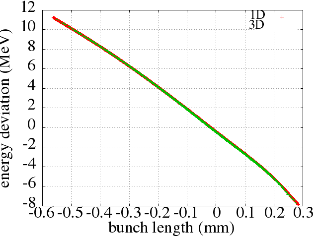
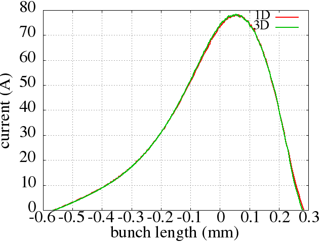
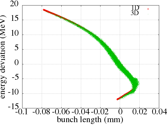
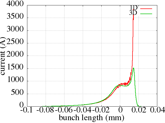
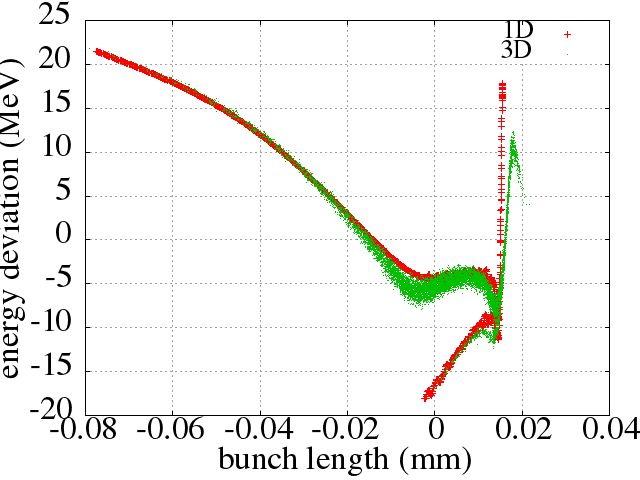
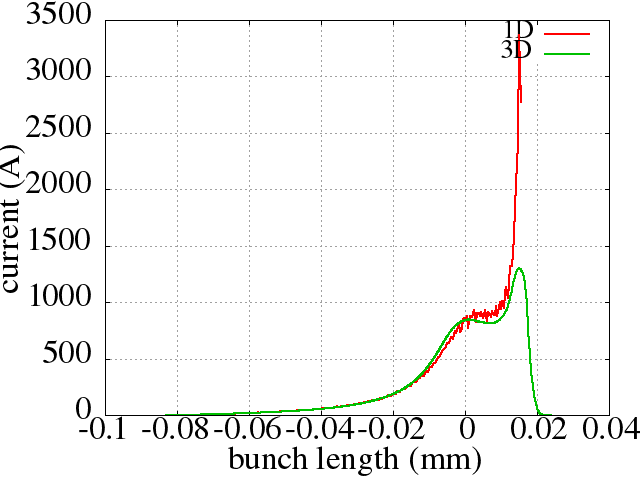
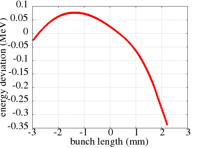
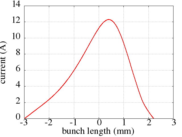
Figure 2 shows the initial longitudinal phase space and current profile at the entrance of the LCLS-II linac. This initial beam distribution has an energy of about $100$ MeV coming out of a high repetition rate photoinjector. A total $1024$ macroparticles (corresponding to $1024$ grid points/slices) that uniformly distributed along the bunch length coordinate are used in the 1D simulation. The energy deviation of each macroparticle can be obtained from the left longitudinal phase space plot of the Fig. 2. The charge weight of each macroparticle can be obtained from the right current plot, i.e. $w_{i}=I_{i}\delta z/c$, where $I_{i}$ is the current at longitudinal bunch position $i$ and $\delta z$ is the longitudinal grid size.

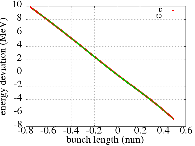
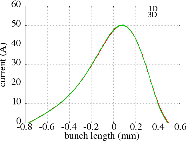
Figure 3 shows the longitudinal phase space and current profile after the magnetic bunch compression chicane BC1 from the tracking using $1024$ macroparticles and the above one-dimensional (1D) longitudinal beam dynamics model and the lumped elements and from the three-dimensional (3D) element-by-element tracking using the IMPACT code with the real number of electrons. In the 1D tracking, the longitudinal space-charge effect and the structure wakefields from the RF cavities are included in the simulation. The CSR effect is applied only through the last bending dipole magnet where the bunch length is short and the CSR effect is strong chad . It is seen that both models agree with each other very well after BC1.

Figure 4 shows the longitudinal phase space and current profile after magnetic bunch compression chicane BC2 from the the above 1D longitudinal beam dynamics model with lumped beam line elements and from the 3D element-by-element multi-particle tracking using the IMPACT code. It is seen that the longitudinal phase space and the current profile from both models agree with each other quite well. The large current spike around the head of the beam from the 1D model is due to the fact that the 1D model started with a distribution with zero uncorrelated energy spread. Such uncorrelated energy spread in the 3D multi-particle simulation smears the longitudinal phase space somewhat and reduces the current spike near the head of the beam. The longitudinal space-charge effect and the RF cavity structure wakefields are included in the 1D tracking. The CSR effect was applied through the last bending magnet of the BC2.

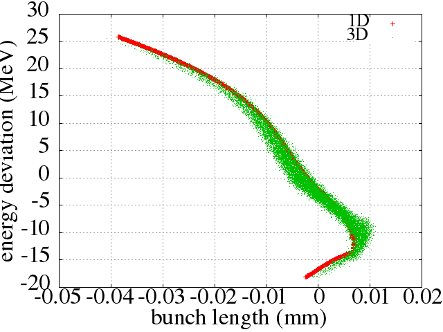
After the bunch compressor BC2, the electron beam moves through another accelerating section (linac 3), a long transport beam line, and a hard x-ray beam transport line, before entering the undulator section. There are a number of dogleg sections in the transport beam line. Here, we included the longitudinal space-charge effect, the structure wakefield in linac3, the CSR effect inside a long bending magnet with a large bending angle, and the resistive wall wakefields. Figure 5 shows the final longitudinal phase space and current profile at the end of accelerator beam delivery system, i.e. at the entrance of undulator section from the above 1D longitudinal beam dynamics model with lumped elements and from the 3D element-by-element tracking using the IMPACT code. The final longitudinal phase space and the current profile from the 1D model agree with those from the 3D model quite well. The longitudinal phase space from the 1D model shows similar shape to that from the 3D model including the fold-over particle distribution near the head of the electron beam. The current spike around the head of the bunch from the 1D model is higher than the spike from the 3D simulation due to the absence of the initial uncorrelated energy spread in the particle distribution.

The benchmark between the above 1D longitudinal beam dynamics model using lumped elements and the 3D element-by-element multi-particle simulation shows good agreement between those two models. This gives us confidence in applying this fast 1D model to final longitudinal phase space optimization to attain high peak current and flat longitudinal phase space distribution.

III Multi-Objective Differential Evolution Optimization Algorithm

In many accelerator applications, one needs to optimize more than one objective function. The problem of multi-objective optimization can be stated in the general mathematical form as:

$$min\left\{\begin{array}[]{l}f_{1}(\vec{x})\\ \cdots\\ f_{n}(\vec{x})\end{array}\right.subject\ to\ g_{i}(\vec{x})\leq 0,h_{i}(\vec{x})=0$$ (30)

Here, $f_{1},\cdots,f_{n}$ are $n$ objective functions to be optimized, $\vec{x}$ is a vector of control parameters, and $g_{i}$ and $h_{i}$ are constraints to the optimization. The goal of multi-objective optimization is to find the Pareto front in the objective function solution space. The Pareto optimal front is a collection of non-dominated solutions in the whole feasible solution space. Any other solution in the feasible solution space will be dominated by those solutions on the Pareto optimal front. In the multi-objective optimization, a solution A is said to dominate a solution B if all components of A are at least as good as those of B (with at least one component strictly better). Here, a component of A corresponds to one objective function value, i.e. $A_{i}=f_{i}(\vec{x})$. The solution A is non-dominated if it is not dominated by any solution within the group.

Recently, we developed a new parallel multi-objective differential evolution algorithm with varying population size of each generation and with external storage to save non-dominated solutions qiangop3 ; qiangop4 . The use of variable population from generation to generation is based on the observation that during the early stage of evolution, the number of nondominated solutions is small. There is no need to keep many dominated solutions in the parent population. As the search evolves, more and more nondominated solutions are obtained. Those nondominated solutions are stored in an external storage so that they can be used for selecting the new parent population. The advantage of using a variable population size with external storage is to reduce the number of objective function evaluations and to improve the speed of convergence. The new algorithm is summarized in the following steps:

• Step 0: Define the minimum parent size, $NPmin$ and the maximum size, $NPmax$ of the parent population. Define the maximum size of the external storage, $NPext$.

• Step 1: An initial $NPini$ population of parameter vectors are chosen quasi-randomly to cover the entire solution space.

• Step 2: Generate the offspring population using a unified differential evolution algorithm.

• Step 3: Check the new population against the constraints.

• Step 4: Combine the new population with the existing parent population from the external storage. Non-dominated solutions ($Ndom$) are found from this group of solutions and $min(Ndom,Next)$ of solutions are put back to the external storage. Pruning is used if $Ndom>Next$. $NP$ parent solutions are selected from this group of solutions for next generation production. If $NPmin\leq Ndom\leq NPmax$, $NP=Ndom$. Otherwise, $NP=NPmin$ if $Ndom<NPmin$ and $NP=NPmax$ if $Ndom>NPmax$. The elitism is emphasized through keeping the non-dominated solutions while the diversity is maintained by penalizing the over-crowded solutions through pruning.

• Step 5: If the stopping condition is met, stop. Otherwise, return to Step 2.

The differential evolution algorithm is a simple but powerful method for global parameter optimization storn2 ; ali ; price . Compared with the other evolutionary algorithms such as the genetic algorithm, the differential evolution algorithm makes use of the differences of parent solutions to attain gradient information. This helps improve the convergence speed of the algorithm in comparison to the genetic algorithm. Meanwhile, compared with the particle swarm method, the differential evolution algorithm has a cross-over stage to enhance the diversity of solutions. This helps the differential evolution algorithm to avoid converging to a premature solution.

The differential evolution algorithm generates new offsprings using two operations: mutation and crossover. During the mutation stage, for each population member (target vector) $\vec{x}_{i}$, $i=1,2,3,\cdots,NP$ at generation $G$, a new mutant vector $\vec{v}_{i}$ is generated by following a mutation strategy. A number of mutation strategies have been proposed for the conventional standard differential evolution algorithm. The presence of multiple mutation strategies complicates the use of the differential evolution algorithm. Recently, we proposed a single mutation expression that can unify most conventional mutation strategies used by the differential evolution algorithm qiangop2 . This single unified mutation strategy can be written as:

$$\vec{v}_{i} = \vec{x}_{i}+F_{1}(\vec{x}_{b}-\vec{x}_{i})+F_{2}(\vec{x}_{r_{1}}-\vec{x}_{i})+F_{3}(\vec{x}_{r_{2}}-\vec{x}_{r_{3}})$$ (31)

Here, the second term on the right-hand side of equation (31) denotes the contribution from the best solution found in the current generation, the third term denotes the rotationally invariant contribution from the random solution price2 , and the fourth term is the same terms as that used in the original differential evolution algorithm to account for the contribution from the difference of parent solutions. Those last two terms divert the mutated solution away from the best solution and help to improve the algorithm’s exploration of the decision parameter space. The three parameters $F_{1}$, $F_{2}$, and $F_{3}$ are the weights from each contribution. This unified expression represents a combination of exploitation (using the best found solution) and exploration (using randomly chosen solutions) when generating the new mutant solution.

Using the equation (31), the multiple mutation strategies of the standard differential evolution algorithm can be included in a single expression. For example, the standard differential evolution algorithm such as DE/rand/1 can be attained by setting $F_{1}=0$, and $F_{2}=1$. This new expression provides an opportunity to explore more broadly the space of mutation operators. Using a different set of parameters $F_{1},F_{2},F_{3}$, a new mutation strategy can be achieved. Moreover, by adjusting these parameters during the evolution, the multiple mutation strategies and their combinations can be used during different stages of optimization. Thus, the unified mutation expression has the virtue of mathematical simplicity and also provides users with flexibility for broader exploration of different mutation strategies.

A crossover operation between the new generated mutant vector $\vec{v}_{i}$ and the target vector $\vec{x}_{i}$ is used to further increase the diversity of the new candidate solution. This operation combines the two vectors into a new trial vector $\vec{U}_{i},i=1,2,3,\cdots,NP$, where the components of the trial vector are obtained from the components of $\vec{v}_{i}$ or $\vec{x}_{i}$ according to a crossover probability $Cr$. In the binomial crossover scheme for a $D$ dimensional control parameter space, the new trial vector $\vec{U}_{i}$, $i=1,2,\cdots,NP$ is generated using the following rule:

$$\vec{U}_{i} = (u_{i1},u_{i2},\cdots,u_{iD})$$ (32)

$$u_{ij} = \left\{\begin{array}[]{ll}v_{ij},&{\rm if}\ \ {\rm rand}_{j}\leq Cr\ \ {\rm or}\ j={\rm mbr}_{i}\\ x_{ij},&{\rm otherwise}\end{array}\right.$$ (35)

where rand_j is a randomly chosen real number in the interval $[0,1]$, and the index $mbr_{i}$ is a randomly chosen integer in the range $[1,D]$. This ensures that the new trial vector contains at least one component from the new mutant vector.

During the mutation stage and the crossover stage at generation, each individual solution $\vec{x}_{i}$, $i=1,2,3,\cdots,NP$ has a set of control parameters $F_{1,i},F_{2,i},F_{3,i}$ and $Cr_{i}$ associated with it. Before generating a new mutant solution using the unified differential evolution expression (31), a set of control parameters $F_{1,i},F_{2,i},F_{3,i}$ and $Cr_{i}$ are calculated as:

$$F_{j,i} = F_{jmin}+r_{ji}(F_{jmax}-F_{jmin})$$ (36)

$$Cr_{i} = Cr_{min}+r_{i}(Cr_{max}-Cr_{min})$$ (37)

where $r_{ji},r_{i},j=1,2,3$ are uniform random values in the interval $[0,1]$, $F_{jmin}$ and $F_{jmax}$ for $j=1,2,3$ are the minimum and the maximum allowed values of those control parameters, $Cr_{min}$ and $Cr_{max}$ are the minimum and the maximum cross-over probability. The values of $F_{jmin}$ and $F_{jmax}$ are set to $0$ and $1$ respectively in this study. We also set $Cr_{min}=0.5$ and $Cr_{max}=1$. The selection of these values is based on the consideration that the various conventional differential evolution mutation strategies can be covered by the settings of those parameters, and in the literature, $F_{3}$ is rarely greater than one.

IV Longitudinal beam dynamics optimization of a LCLS-II design

We applied the above fast one-dimensional longitudinal beam dynamics model together with the multi-objective optimization algorithm to an existing LCLS-II design optimization. The two objective functions in this optimization are the final negative fraction of charge and rms energy spread inside a longitudinal phase space window. Here, the window’s bunch length is set between -$5$ microns and $5$ microns, while the energy spread is set between -$8$ MeV and $8$ MeV. The smaller the negative fraction of charge, the higher the peak current will be. The smaller the rms energy spread inside the window, the flatter the longitudinal phase space will be. In general, the higher peak current might result in the larger energy spread. By simultaneously optimizing those two conflict objectives, we hope to attain the best achievable solutions, i.e. the Pareto optimal front. The high peak current and flat longitudinal phase space improves the x-ray FEL radiation power and reduces the radiation bandwidth.

We used $10$ control parameters of the linear accelerator in this optimization. These $10$ control parameters in the LCLS-II linac are the linac section one RF cavity accelerating gradient amplitude and RF phase, 3rd harmonic cavity amplitude and phase, bending angle in bunch compressor one, linac section two RF cavity amplitude and phase, bending angle in bunch compressor two, and linac three RF cavity amplitude and phase. The maximum RF cavity accelerating gradient is constrained around $16MV/m$ and the final energy around $4$ GeV. The initial population size is $256$. The minimum and the maximum population size are set as $128$ and $1024$ respectively. The maximum number of nondominated solutions in the external storage is set as $2000$. The Pareto front converges after about $460$ generations with about $76$ thousand objective function evaluations. It took one and half hour computing time on $64$ Intel Xeon Phi Processor $7250$ at National Energy Research Supercomputing Center. A major section of the Pareto front (with fraction of charge less than $0.6$) has converged after one hour of computing time after $360$ generations with $51$ thousand function evaluations. Figure 6 shows the Pareto optimal front of the final rms energy spread and the negative fraction of charge inside the defined window from the above multi-objective longitudinal beam dynamics optimization.

Figure 6: The Pareto front of longitudinal phase space optimization.

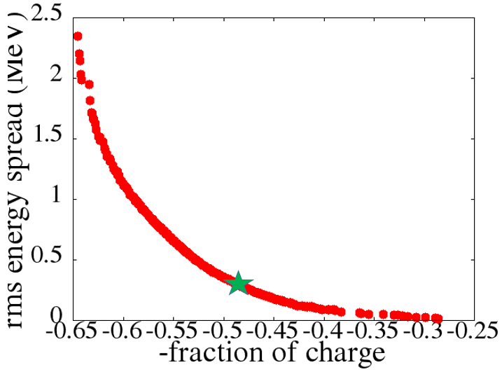
This optimal front suggests that the more charge inside the core of the beam, the larger correlated energy spread the longitudinal phase space will be.

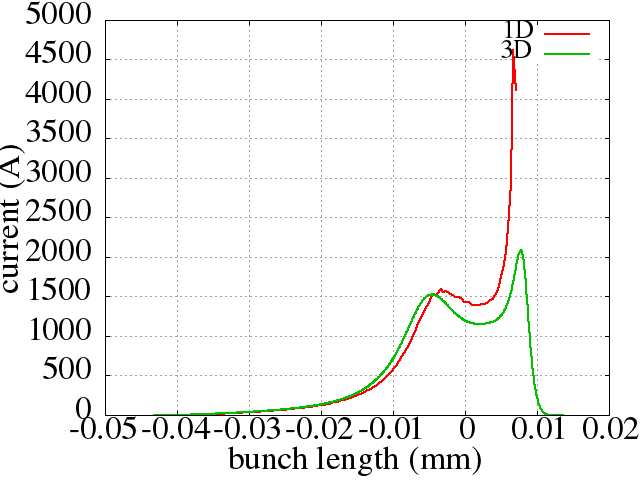
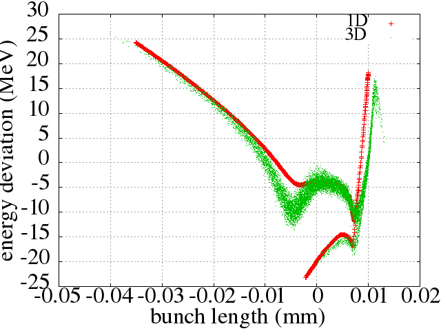
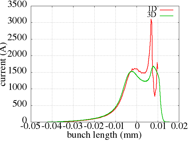
From those optimal solutions, we selected one optimal solution, the green star in Fig. 6. For this solution, the optimized linac one RF cavity accelerating gradient amplitude and phase are $11.5$ M/m and $-14.9$ degrees respectively, harmonic linearizer RF cavity amplitude and phase are $9.0$ M/m and $153.6$ degrees respectively, bunch compression one bending angle is $0.10$ radian, linac two RF cavity amplitude and phase are $16.1$ M/m and -$30.4$ degrees, bunch compressor two bending angle is $0.047$ radian, linac three amplitude and phase are $16.0$ M/m and $0.0$ degrees. With those parameter settings of the LCLS-II linac, we ran the fast 1D longitudinal beam dynamics simulation and the fully 3D element-by-element multi-particle simulation using the IMPACT code. The longitudinal phase spaces and current profiles after BC1, after BC2, and at the entrance to undulator are given in Figs. 7-9. It is seen that the predictions of the 1D longitudinal beam dynamics model agree with those of the 3D model quite well. There is about a factor of four compression after the first bunch compression chicane. After the second bunch compressor chicane, the electron beam is further compressed by more than a factor of $20$. The optimized solution results in a final core peak current greater than $1.2$ kA, which is about $50\%$ improvement from the previous design of around $800$ A peak current. Such a higher core peak current can result in higher x-ray FEL radiation power.

Figure 7: Longitudinal phase space distribution (left) and current profile (right) after BC1 of the LCLS-II linac from the 1D model (red) and from the 3D model (green) using an optimal solution settings.

Figure 8: Longitudinal phase space distribution (left) and current profile (right) after BC2 of the linac from the 1D model (red) and from the 3D model (green) using an optimal solution settings.

Figure 9: Longitudinal phase space distribution (left) and current profile (right) at the entrance to undulator from the 1D model (red) and from the 3D model (green) using an optimal solution settings.

V Conclusions

In this paper, we proposed a lumped one-dimensional longitudinal beam dynamics model that includes nonlinear effects from drift, RF acceleration, magnetic bunch compression, longitudinal space-charge effect, CSR effect, and structure and resistive wall wakefields, for fast longitudinal phase space optimization in x-ray FEL linear accelerators. Benchmarking using a LCLS-II design, this simplified model shows good agreement with the fully 3D element-by-element multi-particle tracking using the IMPACT code. This model, implemented in a recently developed multi-objective differential evolution optimization program, provides a fast computational tool for the longitudinal phase space optimization and resulted in an improved solution on the existing LCLS-II design. In the future study, we plan to apply this tool to the optimization of using control parameters from both the linac parameter setting and the initial longitudinal phase space. Those optimization results will help set up the requirements for the electron beam longitudinal distribution out of a photoinjector in order to achieve the optimal final electron beam quality at the entrance of undulator.

References

- (1) P. Emma, et al., Nature Photon. 4 (2010) 641.
- (2) E. Allaria, et al., Nature Photon. 6 (2012) 699.
- (3) H. Weise and W. Decking, in Proceedings of the 2017 Free Electron Laser Conference, (JACoW, Geneva, 2017), pp. 9 13.
- (4) H. Tanaka et al., A compact x-ray free-electron laser emitting in the sub-angstrom region, Nat. Photonics 6, 540 (2012).
- (5) H.-S. Kang et al., PAL-XFEL technical design report, Pohang Accelerator Laboratory, 2014.
- (6) C. Milne et al., SwissFEL: The Swiss x-ray free electron laser, Appl. Sci. 7, 720 (2017).
- (7) I. Zagorodnov and M. Dohlus, Phys. Rev. ST Accel. Beams 14, 014403, 2011.
- (8) S. DiMitri et al., Physics Reports 539, p.1, 2014.
- (9) P. Emma et al., in Proceedings of the 2014 Free Electron Laser Conference, Basel, Switzerland, (JACoW, Geneva, 2014), pp. 743-747.
- (10) T. O. Raubenheimer et al., in Proceedings of the 2015 Free Electron Laser Conference, Daejeon, Korea, (JACoW, Geneva, 2015), pp. 618 624.
- (11) K.L.F. Bane, P. Emma, LiTrack: A Fast longitudinal phase space tracking Code with graphical user interface, SLAC-PUB-11037, 2005.
- (12) M. Borland, Elegant, APS LS-287, presented at ICAP 2000, Darmstadt, Germany.
- (13) J. Qiang, R. D. Ryne, S. Habib, V. Decyk, J. Comput. Phys. 163, 434, 2000.
- (14) J. Qiang, R. D. Ryne, M. Venturini, A. A. Zholents, and I. V. Pogorelov, Phys. Rev. ST Accel. Beams, vol. 12, 100702, 2009.
- (15) M. Dohlus, T. Limberg, P. Emma, “Bunch compression for linac-based FELs,” in ICFA Beam Dynamics Newsletter, No. 38, p.15, 2005.
- (16) R.W. Hockney, J.W. Eastwood, Computer Simulation Using Particles, Adam Hilger, New York, 1988.
- (17) J. Qiang, S. Lidia, R. D. Ryne, and C. Limborg-Deprey, Phys. Rev. ST Accel. Beams 9, 044204, 2006.
- (18) E.L. Saldin, E.A. Schneidmiller, M.V. Yurkovb Nuclear Instruments and Methods in Physics Research Section A398 (2012) 373.
- (19) J. Qiang, C. Mitchell, R. Ryne., Nuclear Instruments and Methods in Physics Research Section A682 (2012) 49.
- (20) C. Mitchell, J. Qiang, R. Ryne., Nuclear Instruments and Methods in Physics Research Section A715 (2013) 119.
- (21) C. Mitchell, J. Qiang, P. Emma, Phys. Rev. ST Accel. Beams, vol. 16, 060703 (2013).
- (22) R. Storn and K. Price, Journal of Global Optimization 1a1:341-359, (1997).
- (23) M. M. Ali and A. Torn, Computers and Operations Research, Elsevier, no. 31, p. 1703, 2004.
- (24) K. Price et al., Differential Evolution - A Practical Approach to Global Optimization, Springer, Berlin, 2005.
- (25) K. V. Price, ”An introduction to differential evolution,” in New Ideas in Optimization, D. Corne, M. Dorigo, and V. Glover, Eds. London, U.K.: McGraw-Hill, 1999, pp. 79-108.
- (26) J. Qiang et al., in Proceedings of IPAC2013, p. 1031, Shanghai, 2013.
- (27) J. Qiang, “Advances in global optimization of high brightness beams,” to appear in Int. J. Mod. Phys. A, 2019.
- (28) J. Qiang, C. Mitchell, and A. Qiang, in Proc. CEC2016, Vancouver, p. 4061, 2016.