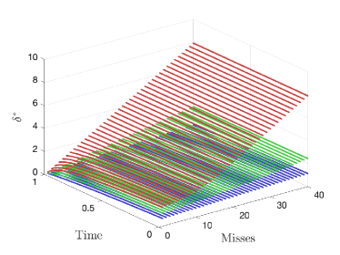
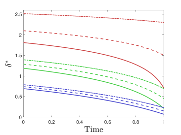
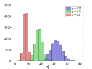
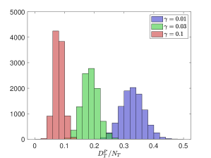
Latency and Liquidity Risk

Álvaro Cartea Mathematical Institute, University of Oxford Oxford-Man Institute of Quantitative Finance alvaro.cartea@maths.ox.ac.uk Department of Statistical Sciences, University of Toronto Sebastian Jaimungal sebastian.jaimungal@utoronto.ca Leandro Sánchez-Betancourt leandro.sanchezbetancourt@maths.ox.ac.uk
Abstract

Latency (i.e., time delay) in electronic markets affects the efficacy of liquidity taking strategies. During the time liquidity takers process information and send marketable limit orders (MLOs) to the exchange, the limit order book (LOB) might undergo updates, so there is no guarantee that MLOs are filled. We develop a latency-optimal trading strategy that improves the marksmanship of liquidity takers. The interaction between the LOB and MLOs is modelled as a marked point process. Each MLO specifies a price limit so the order can receive worse prices and quantities than those the liquidity taker targets if the updates in the LOB are against the interest of the trader. In our model, the liquidity taker balances the tradeoff between missing trades and the costs of walking the book. We employ techniques of variational analysis to obtain the optimal price limit of each MLO the agent sends. The price limit of a MLO is characterized as the solution to a new class of forward-backward stochastic differential equations (FBSDEs) driven by random measures. We prove the existence and uniqueness of the solution to the FBSDE and numerically solve it to illustrate the performance of the latency-optimal strategies.

keywords:
Marked point processes , high-frequency trading , algorithmic trading , latency , forward-backward stochastic differential equations.
journal: TBAlabel0label0footnotetext: SJ would like to acknowledge support from the Natural Sciences and Engineering Research Council of Canada (grants RGPIN-2018-05705 and RGPAS-2018-522715). LSB acknowledges support from CONACyT, México and the Mathematical Institute, University of Oxford.

Introduction

Speed to make decisions and to access the market is a key element in the success of trading strategies in electronic markets. Liquidity providers monitor and update their limit orders (LOs) resting in the limit order book (LOB), and liquidity takers send orders that target LOs. The efficacy of the strategies of the makers and takers of liquidity depends on their latency in the marketplace. Latency is the time delay between an exchange streaming market data to a trader, the trader processing information and making a decision, and the exchange receiving the instruction from the trader. Thus, due to latency, there is no guarantee that liquidity providers can place a LO in a desired queue position in the book or withdraw a stale quote before it is picked off by another trader.

Furthermore, there are no assurances that marketable limit orders (MLOs) from liquidity takers, which aim at a quantity and price they observed in the LOB, hit the desired target. A MLO is a liquidity taking order for immediate execution against the LOs resting in the book, and each MLO specifies the quantity of the security (e.g., equity, currency pairs, futures, etc.) and a price limit to execute against LOs.111A marketable order and a market order differ in that the marketable limit order walks the LOB until it reaches the limit price specified by the trader, while a market order walks the LOB until it is filled in full. Due to latency, by the time the exchange processes a MLO, prices and quantities could have improved, so the order is filled at a better price, or prices and quantities could have worsened, so the order is filled if the limit price allows, otherwise the order is rejected.

In this paper, we focus on how latency affects the marksmanship of liquidity takers and we develop a latency-optimal trading strategy that accounts for the time delays in the marketplace. We frame the interaction between the LOB and MLOs as a marked point process (MPP). In our model, the agent sends buy/sell MLOs at random times to partly camouflage her order flow, and before the order reaches the exchange, the LOB undergoes quantity and price updates. We assume the agent sends fill-or-kill MLOs, that is, the orders are either filled in full or rejected.222This is in contrast to an immediate-or-cancel order, which has the property that the order can be partially filled if there is liquidity in the LOB that meets the requirements of the MLO. The unfilled portion of the order is rejected. The price limit of the MLO consists of the best quote the agent observes at the time she decides to trade and a discretion to walk the LOB.

The LOB is a moving target, so liquidity takers hit or miss the LOs they are attempting to execute. Everything else being the same, the chances of filling a MLO increase if the agent is willing to receive quantities and prices that are worse than those of the best quotes the agent observes in the LOB when she decides to trade. If the discretion to walk the book is unlimited, the MLO will be filled, but potentially at much worse prices than those of the best quotes the agent observed. On the other hand, if the updates in the LOB are in the interest of the agent, the MLO will be filled at better prices than those of the LOs that the agent targeted.

In our model, the agent balances the tradeoff between missing trades and the costs from walking the LOB over a trading window (e.g., minutes, hours, days, etc.). For each liquidity taking order, the strategy optimizes the discretion of the MLO, while it penalizes both the number of missed trades and the costs accrued to the strategy over the trading horizon. We employ techniques of variational analysis to obtain the optimal discretion for each MLO the agent sends, which we characterize as the solution to a forward-backward stochastic differential equation (FBSDE). We show existence and uniqueness of the solution to the forward and backward parts of the FBSDE and show existence and uniqueness of the solution to the full FBSDE. To the best of our knowledge, uniqueness and existence of the resulting random-measure driven FBSDE is not covered in the extant literature, and the particular form itself appears to be new.

In the agent’s performance criterion, when the penalty for missing trades is linear in the expected number of rejected trades, we obtain the optimal strategy in closed-form – the latency-optimal strategy consists of sending all MLOs with a fixed discretion. When the penalty for missing trades is quadratic in the expected number of rejected trades, we solve the FBSDE numerically. We illustrate the performance of the latency-optimal strategies for a range of model parameters and examine the tradeoff between costs from walking the book and number of missed trades. Finally, we discuss strategies that are cost-neutral to the agent. That is, the latency-optimal strategy is devised so the expected costs from walking the book to fill MLOs when the LOB moves against the agent’s interests is the same as the expected benefits (i.e., negative costs) from executing trades at better prices than the ones the agent targets.

Several authors address various aspects of latency in electronic markets. Moallemi and Saĝlam, (2013) look at the cost of latency for liquidity takers in equity markets. They compare the costs of liquidating one stock with and without time delays in the marketplace to compute the cost of latency. The work of Stoikov and Waeber, (2016) shows how to execute a large order in electronic markets by employing the volume imbalance of the LOB to predict price changes and study the effect of latency in the efficacy of the execution strategy. Lehalle and Mounjid, (2017) employ data from Nasdaq-Omx and also find that as latency increases, the informational content in the volumes of the LOB diminishes.

Cartea and Sánchez-Betancourt, (2018) employ proprietary foreign exchange data to show how latency and volatility of the midprice of the security affect the fill ratio of liquidity taking strategies. The authors show how traders could employ latency-optimal strategies to improve fill ratios, while minimizing costs, and they show how to compute the shadow price of latency in foreign exchange markets. Gao and Wang, (2018) use Markov decision processes to model the problem of a market maker with latency who trades in a LOB, where the size of the quoted spread is always one tick. The authors find that as latency increases, the profits from making markets decrease.

Recent literature on high-frequency trading and algorithmic trading discusses various characteristics of trading and how traders use speed to obtain informational advantages, see e.g., Lehalle and Laruelle, (2013). Other strands of the literature discuss the relationship of market quality, the speed of market participants, and stochastic liquidity, see for example Almgren, (2012) and Guéant, (2016) for trading in illiquid markets. Barger and Lorig, (2019) model the rapid updates of the best quotes in the LOB to propose a model of stochastic price impact.

The remainder of the paper proceeds as follows. Section 2 proposes the agent’s performance criterion and characterizes the latency-optimal strategy as the solution to a FBSDE. Section 3 shows existence and uniqueness of the solution of the forward and backward part of the FBSDE, and existence and uniqueness of the solution to the full FBSDE. Section 4 shows that the candidate control we find is the global optimum and Section 5 discusses the performance of the strategy for various scenarios. We conclude in Section 6 and collect some proofs in the Appendix.

Optimal discretion to walk the book

Latency: the LOB as a moving target

Liquidity takers in electronic markets face a moving target problem. Traders send orders that target a price and quantity they observe in the LOB, but due to latency, when the order arrives in the exchange, the target could have moved. If prices and quantities worsen, the agent’s order is rejected, and if prices and quantities improve or do not worsen, the order is filled.

We frame the moving target problem as a MPP 𝒩={(Tn,Zn)}(n1)𝒩subscriptsubscript𝑇𝑛subscript𝑍𝑛𝑛1\mathcal{N}=\{(T_{n},\,Z_{n})\}_{(n\geq 1)} in the probability space (Ω,,)Ω\left(\Omega,\,\mathcal{F},\,\mathbb{P}\right). Here, (Tn)subscript𝑇𝑛(T_{n}) is an increasing sequence of random points in (0,T]{}0𝑇(0,T]\bigcup\{\infty\}, which represent the times when the agent sends MLOs to the exchange, and (Zn)subscript𝑍𝑛(Z_{n}) is a sequence of marks, which represent the shock to the average price per share due to changes in prices and quantities.

We assume that each order is for one unit of the security or for a lot of securities, where the lots have a fixed size throughout the trading horizon. When the volume of the MLO is in lots of the security, the mark Z𝑍Z represents a shock to the LOB commensurate with the volume of the MLO.

As in Confortola et al., (2016), we define the sample space to be Ω=n{Tn>T}Ωsubscript𝑛subscript𝑇𝑛𝑇\Omega={\bigcup}_{n}\{T_{n}>T\}, where T(0,)𝑇0T\in(0,\infty) denotes a fixed time horizon. The filtration (t)t0subscriptsubscript𝑡𝑡0\left(\mathcal{F}_{t}\right)_{t\geq 0} is generated by 𝒩𝒩\mathcal{N} and is the smallest filtration such that for each n𝑛n, the point Tnsubscript𝑇𝑛T_{n} is a stopping time and the mark Znsubscript𝑍𝑛Z_{n} is Tnsubscriptsubscript𝑇𝑛\mathcal{F}_{T_{n}}-measurable. We use predictable processes to mean the left-continuous version of a process, see Theorem 7.2.4 in Cohen and Elliott, (2015).

The random measure associated with 𝒩𝒩\mathcal{N} is

p(dt,dz)=n1:TnT𝔇(Tn,Zn)(dt,dz),𝑝d𝑡d𝑧subscript:𝑛1subscript𝑇𝑛𝑇subscript𝔇subscript𝑇𝑛subscript𝑍𝑛d𝑡d𝑧p(\mathrm{d}t,\mathrm{d}z)=\sum_{n\geq 1:T_{n}\leq T}\mathfrak{D}_{(T_{n},Z_{n})}(\mathrm{d}t,\mathrm{d}z)\,,

where 𝔇𝔇\mathfrak{D} denotes the Dirac measure, and we assume that

𝔼[(p([0,T],))2]<and𝔼[0T|z|p(dz,dt)]<.formulae-sequence𝔼delimited-[]superscript𝑝0𝑇2and𝔼delimited-[]superscriptsubscript0𝑇subscript𝑧𝑝d𝑧d𝑡\mathbb{E}\left[\left(p\left([0,T],\,\mathbb{R}\right)\right)^{2}\right]<\infty\qquad\text{and}\qquad\mathbb{E}\left[\int_{0}^{T}\int_{\mathbb{R}}\left|z\right|\,p(\mathrm{d}z,\mathrm{d}t)\right]<\infty\,. (1)

We denote by p~~𝑝\tilde{p} the predictable compensator of the random measure p𝑝p, which admits the following decomposition

p~(dz,dt)=ϕt(dz)dAt.~𝑝d𝑧d𝑡subscriptitalic-ϕ𝑡d𝑧dsubscript𝐴𝑡\tilde{p}(\mathrm{d}z,\mathrm{d}t)=\phi_{t}(\mathrm{d}z)\,\mathrm{d}A_{t}\,. (2)

Here, the compensator has the property that for q:=pp~assign𝑞𝑝~𝑝q:=p-\tilde{p} and any integrable and predictable process H𝐻H, the stochastic integral (Hq)t=0tHsq(ds,dz)subscript𝐻𝑞𝑡superscriptsubscript0𝑡subscriptsubscript𝐻𝑠𝑞d𝑠d𝑧\left(H\star q\right)_{t}=\int_{0}^{t}\int_{\mathbb{R}}H_{s}\,q(\mathrm{d}s,\mathrm{d}z) is a martingale. In (2), the predictable process (At)t𝔗subscriptsubscript𝐴𝑡𝑡𝔗(A_{t})_{t\in{\mathfrak{T}}}, where 𝔗:=[0,T]assign𝔗0𝑇{\mathfrak{T}}:=[0,T], is the compensator of the counting process of the MLOs, which we denote by Nt:=p([0,t]×)assignsubscript𝑁𝑡𝑝0𝑡N_{t}:=p([0,t]\times\mathbb{R}).

Assumption 1.

The process A𝐴A admits a bounded stochastic intensity so that we may write At=0tλudusubscript𝐴𝑡superscriptsubscript0𝑡subscript𝜆𝑢differential-d𝑢A_{t}=\int_{0}^{t}\lambda_{u}\,\mathrm{d}u for a predictable process (λt)t𝔗subscriptsubscript𝜆𝑡𝑡𝔗\left(\lambda_{t}\right)_{{t\in{\mathfrak{T}}}} and λ¯¯𝜆\exists\,\,\bar{\lambda}\in\mathbb{R}, such that (t,ω)[0,T]×Ωfor-all𝑡𝜔0𝑇Ω\forall\,(t,\omega)\in[0,T]\times\Omega, λt(ω)λ¯subscript𝜆𝑡𝜔¯𝜆\lambda_{t}(\omega)\leq\bar{\lambda}.

The density function of the marks is ϕtsubscriptitalic-ϕ𝑡\phi_{t}, which has support in \mathbb{R} and is bounded, and its cumulative distribution function is ΦtsubscriptΦ𝑡\Phi_{t}, which we assume is uniformly Lipchitz in [0,T]×Ω0𝑇Ω[0,T]\times\Omega with Lipschitz constant k𝑘k.

Let (δt)t𝔗subscriptsubscript𝛿𝑡𝑡𝔗\left(\delta_{t}\right)_{{t\in{\mathfrak{T}}}} be a predictable process that specifies the cash per unit of the security (or lots of the security) the agent is willing to walk the LOB to increase the chances of filling her liquidity taking order, i.e., δ𝛿\delta is the discretion of the MLO. For example, in equity markets, if the agent sends a buy order to lift the offer at the best ask atsubscript𝑎𝑡a_{t}, the discretionary amount δtsubscript𝛿𝑡\delta_{t} is the extra cash per share the order may walk the book, i.e., at+δtsubscript𝑎𝑡subscript𝛿𝑡a_{t}+\delta_{t} is the highest price the agent is willing to pay for one share of equity. Similarly, if the agent sends a sell order to hit the best bid btsubscript𝑏𝑡b_{t}, the amount δtsubscript𝛿𝑡\delta_{t} is the cash discount per share the order may walk the book, i.e., btδtsubscript𝑏𝑡subscript𝛿𝑡b_{t}-\delta_{t} is the lowest price the agent is willing to accept to sell one share of equity.

In the examples above, the best bid and best ask prices (btsubscript𝑏𝑡b_{t} and atsubscript𝑎𝑡a_{t}) refer to those the agent ‘observes’ when she decides to trade, but due to latency, these prices could be stale. In addition, by the time the exchange processes the order of the agent, prices and quantities in the LOB could have borne further updates. Price changes could be against or in favour of the agent’s interest. When the price per unit of the security moves against the interest of the agent, the order is filled only if the discretion δ𝛿\delta of the MLO is enough to cover the adverse change in price and quantity; we refer to this as a price deterioration. On the other hand, if the price per unit of the security moves in favour of the agent’s trade interest, the order is filled at a better price; we refer to this as a price improvement

Tradeoff: cost of walking the LOB and missed trades

The agent must balance the costs of walking the LOB against the number of missed trades as a consequence of her latency in the marketplace. Clearly, if the agent sends orders with infinite discretion to walk the LOB, all orders are filled (we rule out cases in which the LOB is empty) and the costs accrued from walking the LOB are expected to be highest. On the other hand, everything else being equal, lowering discretion, lowers the strategy’s cost but increases the number of missed trades.

We discuss the cost for MLOs with volume equal to one unit of the security – the costs for MLOs where volume is in lots of the security are computed in a similar way. For buy orders, the cost of the strategy is the cash the agent pays for the security minus the price on the offer side of the LOB that the agent targets. Similarly, for sell orders, the cost of the strategy is the target price in the bid side of the LOB minus the cash received for the security. That is, the cost of the strategy is the extra cash paid to walk the LOB, which is zero if the order is not executed. We denote the controlled cost process by Cδ=(Cδ)t𝔗superscript𝐶𝛿subscriptsuperscript𝐶𝛿𝑡𝔗C^{\delta}=(C^{\delta})_{{t\in{\mathfrak{T}}}} and

Ctδ=0tzG^(δsz)p(dz,ds),subscriptsuperscript𝐶𝛿𝑡superscriptsubscript0𝑡subscript𝑧^𝐺subscript𝛿𝑠𝑧𝑝d𝑧d𝑠C^{\delta}_{t}=\int_{0}^{t}\int_{\mathbb{R}}z\,{\hat{G}}(\delta_{s}-z)\,p(\mathrm{d}z,\mathrm{d}s)\,, (3)

where G^(x)=1^𝐺𝑥1{\hat{G}}(x)=1 if x0𝑥0x\geq 0 and G^(x)=0^𝐺𝑥0{\hat{G}}(x)=0 otherwise.

The extra cost for each filled trade is zG^(δsz)𝑧^𝐺subscript𝛿𝑠𝑧z\,{\hat{G}}(\delta_{s}-z), which can be negative (price improvement), positive (price deterioration), or zero. This cost is negative when the shock to the LOB is negative (z<0𝑧0z<0), in which case the order is filled at a better price than that targeted by the agent – the price improvement is |z|𝑧\left|z\right|. On the other hand, this cost is positive when the shock to the LOB is positive (z>0𝑧0z>0), in which case the order is filled (because δz𝛿𝑧\delta\geq z) at a worse price than that targeted by the agent – the price deterioration is z𝑧z. Finally, when the shock to the LOB is zero (z=0𝑧0z=0) or the trade is missed, the cost is zero.

The process Dδ=(Dtδ)t𝔗superscript𝐷𝛿subscriptsubscriptsuperscript𝐷𝛿𝑡𝑡𝔗D^{\delta}=(D^{\delta}_{t})_{{t\in{\mathfrak{T}}}} denotes the controlled number of misses and

Dtδ=0tG(δsz)p(dz,ds),subscriptsuperscript𝐷𝛿𝑡superscriptsubscript0𝑡subscript𝐺subscript𝛿𝑠𝑧𝑝d𝑧d𝑠D^{\delta}_{t}=\int_{0}^{t}\int_{\mathbb{R}}G\left(\delta_{s}-z\right)\,p(\mathrm{d}z,\mathrm{d}s)\,, (4)

where G(x)=1G^(x)𝐺𝑥1^𝐺𝑥G(x)=1-{\hat{G}}(x). Recall that the MLO is for one unit of the security or for lots of the security, which are of fixed size throughout the trading horizon. In the latter case, the number of misses is in lots of the security.

Performance criterion

The agent’s performance criterion is

J(δ)=𝔼[CTδ+αDTδ+γ(DTδ)2],𝐽𝛿𝔼delimited-[]subscriptsuperscript𝐶𝛿𝑇𝛼subscriptsuperscript𝐷𝛿𝑇𝛾superscriptsubscriptsuperscript𝐷𝛿𝑇2J(\delta)=\mathbb{E}\left[C^{\delta}_{T}+\alpha\,D^{\delta}_{T}+\gamma\,\left(D^{\delta}_{T}\right)^{2}\right]\,, (5)

where both α0𝛼0\alpha\geq 0 and γ0𝛾0\gamma\geq 0 are penalty parameters for the total number of missed trades, and the set of admissible strategies is

𝒜:={δ=(δt)t𝔗|δ is predictable and 𝔼[supt𝔗(δt)2]<}.assign𝒜conditional-set𝛿subscriptsubscript𝛿𝑡𝑡𝔗𝛿 is predictable and 𝔼delimited-[]subscriptsupremum𝑡𝔗superscriptsubscript𝛿𝑡2{\mathcal{A}}:=\left\{\delta=\left(\delta_{t}\right)_{{t\in{\mathfrak{T}}}}\left|\delta\text{ is }\mathcal{F}-\text{{predictable} and }\mathbb{E}\left[\sup_{{t\in{\mathfrak{T}}}}\left(\delta_{t}\right)^{2}\right]\,<\,\infty\right.\right\}\,. (6)

The agent wishes to find a control δ𝒜superscript𝛿𝒜\delta^{*}\in{\mathcal{A}} that minimizes the performance criterion (5), that is, the agent solves the problem

δ=argminδ𝒜J(δ).superscript𝛿subscriptargmin𝛿𝒜𝐽𝛿\delta^{*}=\operatorname*{argmin}_{\delta\in{\mathcal{A}}}J(\delta)\,.

Note that J(δ)<𝐽𝛿J(\delta)<\infty because G1𝐺1G\leq 1 and (1) holds. We choose the units of the parameters α,γ𝛼𝛾\alpha,\,\gamma, so that the performance criterion has the same units as those of the costs C𝐶C.

In the performance criterion, the penalties for missing trades are not financial costs. Everything else being equal, an increase in the value of the penalty parameters makes the strategy post orders with higher discretion to walk the LOB. In the extreme case where one of the penalty parameters is arbitrarily large, the optimal strategy is to post orders with discretion to walk the LOB as deep as necessary to fill the trades, i.e., the MLO with infinite discretion is a market order.

Variational Analysis Approach

We employ techniques of variational analysis to obtain the optimal discretion strategy. For ease of presentation, we write

J(δ)=JC(δ)+αJLP(δ)+γJQP(δ),𝐽𝛿superscript𝐽C𝛿𝛼superscript𝐽LP𝛿𝛾superscript𝐽QP𝛿J(\delta)=J^{\text{C}}(\delta)+\alpha\,J^{\text{LP}}(\delta)+\gamma\,J^{\text{QP}}(\delta)\,, (7)

where JC(δ)=𝔼[CTδ]superscript𝐽C𝛿𝔼delimited-[]subscriptsuperscript𝐶𝛿𝑇J^{\text{C}}(\delta)=\mathbb{E}\left[C^{\delta}_{T}\right], JLP(δ)=𝔼[DTδ]superscript𝐽LP𝛿𝔼delimited-[]subscriptsuperscript𝐷𝛿𝑇J^{\text{LP}}(\delta)=\mathbb{E}\left[D^{\delta}_{T}\right], and JQP(δ)=𝔼[(DTδ)2]superscript𝐽QP𝛿𝔼delimited-[]superscriptsubscriptsuperscript𝐷𝛿𝑇2J^{\text{QP}}(\delta)=\mathbb{E}\left[\left(D^{\delta}_{T}\right)^{2}\right].

Next, note that

JC(δ)superscript𝐽C𝛿\displaystyle J^{\text{C}}(\delta) =𝔼[0TzG^(δtz)p(dz,ds)]=𝔼[0TzG^(δtz)ϕt(dz)dAt],absent𝔼delimited-[]superscriptsubscript0𝑇subscript𝑧^𝐺subscript𝛿𝑡𝑧𝑝d𝑧d𝑠𝔼delimited-[]superscriptsubscript0𝑇subscript𝑧^𝐺subscript𝛿𝑡𝑧subscriptitalic-ϕ𝑡d𝑧differential-dsubscript𝐴𝑡\displaystyle=\mathbb{E}\left[\int_{0}^{T}\int_{\mathbb{R}}z\,{\hat{G}}(\delta_{t}-z)\,p(\mathrm{d}z,\mathrm{d}s)\right]=\mathbb{E}\left[\int_{0}^{T}\int_{\mathbb{R}}z\,{\hat{G}}(\delta_{t}-z)\,\phi_{t}(\mathrm{d}z)\,\mathrm{d}A_{t}\right]\,, (8)

and the next proposition provides expressions for JLP(δ)superscript𝐽𝐿𝑃𝛿J^{LP}(\delta) and JQP(δ)superscript𝐽𝑄𝑃𝛿J^{QP}(\delta).

Proposition 1.

The following equations hold

JLP(δ)superscript𝐽LP𝛿\displaystyle J^{\text{LP}}(\delta) =𝔼[0TG(δtz)p~(dz,dt)],absent𝔼delimited-[]superscriptsubscript0𝑇subscript𝐺subscript𝛿𝑡𝑧~𝑝d𝑧d𝑡\displaystyle=\mathbb{E}\left[\int_{0}^{T}\int_{\mathbb{R}}G(\delta_{t}-z)\,\tilde{p}(\mathrm{d}z,\,\mathrm{d}t)\right]\,, (9)
JQP(δ)superscript𝐽QP𝛿\displaystyle J^{\text{QP}}(\delta) =𝔼[0T(2DtδG(δtz)+G(δtz))p~(dz,dt)].absent𝔼delimited-[]superscriptsubscript0𝑇subscript2subscriptsuperscript𝐷𝛿superscript𝑡𝐺subscript𝛿𝑡𝑧𝐺subscript𝛿𝑡𝑧~𝑝d𝑧d𝑡\displaystyle=\mathbb{E}\left[\int_{0}^{T}\int_{\mathbb{R}}\left(2\,D^{\delta}_{t^{-}}\,G(\delta_{t}-z)+G(\delta_{t}-z)\right)\,\tilde{p}(\mathrm{d}z,\,\mathrm{d}t)\right]\,. (10)
Proof.

Equation (9) follows from the predictability of the integrand. Next, we show (10). The number of missed trades Dtδsubscriptsuperscript𝐷𝛿𝑡D^{\delta}_{t} satisfy the SDE

dDtδ=G(δtz)p(dz,dt).dsubscriptsuperscript𝐷𝛿𝑡subscript𝐺subscript𝛿𝑡𝑧𝑝d𝑧d𝑡\mathrm{d}D^{\delta}_{t}=\int_{\mathbb{R}}G(\delta_{t}-z)\,p(\mathrm{d}z,\,\mathrm{d}t)\,.

Let h(x)=x2𝑥superscript𝑥2h(x)=x^{2} and use an integration formula (see Jeanblanc et al., (2009)) to write

dh(Dtδ)=(h(Dtδ+G(δtz))h(Dtδ))p(dz,dt).dsubscriptsuperscript𝐷𝛿𝑡subscriptsubscriptsuperscript𝐷𝛿superscript𝑡𝐺subscript𝛿𝑡𝑧subscriptsuperscript𝐷𝛿superscript𝑡𝑝d𝑧d𝑡\displaystyle\mathrm{d}h(D^{\delta}_{t})=\int_{\mathbb{R}}\left(h\left(D^{\delta}_{t^{-}}+G\left(\delta_{t}-z\right)\right)-h\left(D^{\delta}_{t^{-}}\right)\right)\,p(\mathrm{d}z,\,\mathrm{d}t)\,.

Then,

d(Dtδ)2dsuperscriptsubscriptsuperscript𝐷𝛿𝑡2\displaystyle\mathrm{d}\left(D^{\delta}_{t}\right)^{2} =(2DtδG(δtz)+G2(δtz))p(dz,dt)absentsubscript2subscriptsuperscript𝐷𝛿superscript𝑡𝐺subscript𝛿𝑡𝑧superscript𝐺2subscript𝛿𝑡𝑧𝑝d𝑧d𝑡\displaystyle=\int_{\mathbb{R}}\left(2\,D^{\delta}_{t^{-}}\,G(\delta_{t}-z)+G^{2}(\delta_{t}-z)\right)\,p(\mathrm{d}z,\,\mathrm{d}t)
=(2DtδG(δtz)+G(δtz))p(dz,dt),absentsubscript2subscriptsuperscript𝐷𝛿superscript𝑡𝐺subscript𝛿𝑡𝑧𝐺subscript𝛿𝑡𝑧𝑝d𝑧d𝑡\displaystyle=\int_{\mathbb{R}}\left(2\,D^{\delta}_{t^{-}}\,G(\delta_{t}-z)+G(\delta_{t}-z)\right)\,p(\mathrm{d}z,\,\mathrm{d}t)\,,

where the second equality holds because G2=Gsuperscript𝐺2𝐺G^{2}=G. Integrate from zero to T𝑇T, take expectations, and because the integrand 2DtδG(δtz)+G(δtz)2subscriptsuperscript𝐷𝛿superscript𝑡𝐺subscript𝛿𝑡𝑧𝐺subscript𝛿𝑡𝑧2\,D^{\delta}_{t^{-}}\,G(\delta_{t}-z)+G(\delta_{t}-z) is predictable, obtain

𝔼[(DTδ)2]𝔼delimited-[]superscriptsubscriptsuperscript𝐷𝛿𝑇2\displaystyle\mathbb{E}\left[\left(D^{\delta}_{T}\right)^{2}\right] =𝔼[0T(2DtδG(δtz)+G(δtz))p(dz,dt)]absent𝔼delimited-[]superscriptsubscript0𝑇subscript2subscriptsuperscript𝐷𝛿superscript𝑡𝐺subscript𝛿𝑡𝑧𝐺subscript𝛿𝑡𝑧𝑝d𝑧d𝑡\displaystyle=\mathbb{E}\left[\int_{0}^{T}\int_{\mathbb{R}}\left(2\,D^{\delta}_{t^{-}}\,G(\delta_{t}-z)+G(\delta_{t}-z)\right)\,p(\mathrm{d}z,\,\mathrm{d}t)\right]
=𝔼[0T(2DtδG(δtz)+G(δtz))p~(dz,dt)].absent𝔼delimited-[]superscriptsubscript0𝑇subscript2subscriptsuperscript𝐷𝛿superscript𝑡𝐺subscript𝛿𝑡𝑧𝐺subscript𝛿𝑡𝑧~𝑝d𝑧d𝑡\displaystyle=\mathbb{E}\left[\int_{0}^{T}\int_{\mathbb{R}}\left(2\,D^{\delta}_{t^{-}}\,G(\delta_{t}-z)+G(\delta_{t}-z)\right)\,\tilde{p}(\mathrm{d}z,\,\mathrm{d}t)\right]\,.


Optimal discretion to walk the LOB

We employ Gâteaux derivatives to obtain the latency-optimal strategy that minimizes the performance criterion of the agent. Let w,δ𝒜𝑤𝛿𝒜w,\delta\,\in\,{\mathcal{A}}. The directional derivative of J𝐽J at δ𝛿\delta in the direction of w𝑤w is given by

𝒟J(δ),w=limϵ01ϵ[J(δ+ϵw)J(δ)],𝒟𝐽𝛿𝑤subscriptitalic-ϵ01italic-ϵdelimited-[]𝐽𝛿italic-ϵ𝑤𝐽𝛿\langle\mathcal{D}\,J(\delta),w\rangle=\lim_{\epsilon\to 0}\tfrac{1}{\epsilon}\left[J(\delta+\epsilon\,w)-J(\delta)\right]\,, (11)

when the limit exists. Now, let 𝒜superscript𝒜{\mathcal{A}}^{\prime} be the dual space of 𝒜𝒜{\mathcal{A}}. If there is A𝒜superscript𝐴superscript𝒜A^{\prime}\in{\mathcal{A}}^{\prime} such that 𝒟J(δ),w=A(w)𝒟𝐽𝛿𝑤superscript𝐴𝑤\langle\mathcal{D}\,J(\delta),w\rangle=A^{\prime}(w) for all w𝒜𝑤𝒜w\in{\mathcal{A}}, then Asuperscript𝐴A^{\prime} is called the Gâteaux derivative of J𝐽J at δ𝛿\delta. In this paper, the directional derivatives are elements of the dual of 𝒜𝒜{\mathcal{A}}, hence we refer to the directional derivatives as Gâteaux derivatives. Note that it is trivial to show that 𝒜𝒜{\mathcal{A}} is a linear space over \mathbb{R}.

Lemma 1.

The Gâteaux derivative at δ𝒜𝛿𝒜\delta\in{\mathcal{A}} in the direction w𝒜𝑤𝒜w\in{\mathcal{A}} of the:

  1. (a)

    cost functional JCsuperscript𝐽CJ^{\text{C}} is

    𝒟JC(δ),w𝒟superscript𝐽C𝛿𝑤\displaystyle\langle\mathcal{D}\,J^{\text{C}}(\delta),w\rangle =𝔼[0Twtϕt(δt)δtdAt];absent𝔼delimited-[]superscriptsubscript0𝑇subscript𝑤𝑡subscriptitalic-ϕ𝑡subscript𝛿𝑡subscript𝛿𝑡differential-dsubscript𝐴𝑡\displaystyle=\mathbb{E}\left[\int_{0}^{T}w_{t}\,\phi_{t}(\delta_{t})\,\delta_{t}\,\mathrm{d}A_{t}\right]\,;
  2. (b)

    linear penalty functional JLPsuperscript𝐽LPJ^{\text{LP}} is

    𝒟JLP(δ),w𝒟superscript𝐽LP𝛿𝑤\displaystyle\langle\mathcal{D}\,J^{\text{LP}}(\delta),w\rangle =𝔼[0Twtϕt(δt)dAt];absent𝔼delimited-[]superscriptsubscript0𝑇subscript𝑤𝑡subscriptitalic-ϕ𝑡subscript𝛿𝑡differential-dsubscript𝐴𝑡\displaystyle=-\mathbb{E}\left[\int_{0}^{T}w_{t}\,\phi_{t}(\delta_{t})\,\mathrm{d}A_{t}\right]\,;
  3. (c)

    quadratic penalty functional JQPsuperscript𝐽QPJ^{\text{QP}} is

    𝒟JQP(δ),w𝒟superscript𝐽QP𝛿𝑤\displaystyle\langle\mathcal{D}\,J^{\text{QP}}(\delta),w\rangle =2𝔼[0Twtϕt(δt)𝔼t[tTG(δsz)p~(dz,ds)]dAt]absent2𝔼delimited-[]superscriptsubscript0𝑇subscript𝑤𝑡subscriptitalic-ϕ𝑡subscript𝛿𝑡subscript𝔼superscript𝑡delimited-[]superscriptsubscript𝑡𝑇subscript𝐺subscript𝛿𝑠superscript𝑧~𝑝dsuperscript𝑧d𝑠differential-dsubscript𝐴𝑡\displaystyle=-2\,\mathbb{E}\left[\int_{0}^{T}w_{t}\,\phi_{t}(\delta_{t})\,\mathbb{E}_{t^{-}}\left[\int_{t}^{T}\int_{\mathbb{R}}G(\delta_{s}-z^{\prime})\,\tilde{p}(\mathrm{d}z^{\prime},\,\mathrm{d}s)\right]\,\mathrm{d}A_{t}\right]
    2𝔼[0Twtϕt(δt)DtδdAt]𝔼[0Twtϕt(δt)dAt].2𝔼delimited-[]superscriptsubscript0𝑇subscript𝑤𝑡subscriptitalic-ϕ𝑡subscript𝛿𝑡subscriptsuperscript𝐷𝛿superscript𝑡differential-dsubscript𝐴𝑡𝔼delimited-[]superscriptsubscript0𝑇subscript𝑤𝑡subscriptitalic-ϕ𝑡subscript𝛿𝑡differential-dsubscript𝐴𝑡\displaystyle\quad-2\,\mathbb{E}\left[\int_{0}^{T}w_{t}\,\phi_{t}(\delta_{t})\,D^{\delta}_{t^{-}}\,\mathrm{d}A_{t}\right]-\mathbb{E}\left[\int_{0}^{T}w_{t}\,\phi_{t}(\delta_{t})\,\mathrm{d}A_{t}\right]\,.
Proof.

See A.  

The next theorem provides the Gâteaux derivative of the performance criterion of the agent and provides a characterization of the optimal discretion to walk the LOB.

Theorem 1.

The Gâteaux derivative of the functional J𝐽J at δ𝒜𝛿𝒜\delta\in{\mathcal{A}} in the direction of w𝒜𝑤𝒜w\in{\mathcal{A}} is

𝒟J(δ),w=𝔼[0Twtϕt(δt)(δt2γDtδγα2γ𝔼t[tTG(δsz)p~(dz,ds)])dAt],𝒟𝐽𝛿𝑤𝔼delimited-[]superscriptsubscript0𝑇subscript𝑤𝑡subscriptitalic-ϕ𝑡subscript𝛿𝑡subscript𝛿𝑡2𝛾subscriptsuperscript𝐷𝛿superscript𝑡𝛾𝛼2𝛾subscript𝔼superscript𝑡delimited-[]superscriptsubscript𝑡𝑇subscript𝐺subscript𝛿𝑠superscript𝑧~𝑝dsuperscript𝑧d𝑠differential-dsubscript𝐴𝑡\displaystyle\langle\mathcal{D}\,J(\delta),w\rangle=\mathbb{E}\left[\int_{0}^{T}w_{t}\,\phi_{t}(\delta_{t})\,\left(\delta_{t}-2\,\gamma\,D^{\delta}_{t^{-}}-\gamma-\alpha-2\,\gamma\,\mathbb{E}_{t^{-}}\left[\int_{t}^{T}\int_{\mathbb{R}}G(\delta_{s}-z^{\prime})\,\tilde{p}(\mathrm{d}z^{\prime},\,\mathrm{d}s)\right]\right)\,\mathrm{d}A_{t}\right]\,,

and vanishes in every direction w𝒜𝑤𝒜w\in{\mathcal{A}} if and only if there is a process δ𝒜superscript𝛿𝒜\delta^{*}\in{\mathcal{A}} such that

δtsubscriptsuperscript𝛿𝑡\displaystyle\delta^{*}_{t} =2γ𝔼t[DTδ]+γ+α,absent2𝛾subscript𝔼superscript𝑡delimited-[]subscriptsuperscript𝐷superscript𝛿𝑇𝛾𝛼\displaystyle=2\,\gamma\,\mathbb{E}_{t^{-}}\left[D^{\delta^{*}}_{T}\right]+\gamma+\alpha\,, (12)

almost everywhere in 𝔗×Ω𝔗Ω{\mathfrak{T}}\times\Omega.

Proof.

By Lemma 1 and the performance criterion (7), the Gâteaux derivative of J𝐽J vanishes at

δtsubscriptsuperscript𝛿𝑡\displaystyle\delta^{*}_{t} =2γ𝔼t[tTG(δsz)p~(dz,ds)]+2γ(Dtδ+12)+αabsent2𝛾subscript𝔼superscript𝑡delimited-[]superscriptsubscript𝑡𝑇subscript𝐺subscriptsuperscript𝛿𝑠superscript𝑧~𝑝dsuperscript𝑧d𝑠2𝛾subscriptsuperscript𝐷superscript𝛿superscript𝑡12𝛼\displaystyle=2\,\gamma\,\mathbb{E}_{t^{-}}\left[\int_{t}^{T}\int_{\mathbb{R}}G(\delta^{*}_{s}-z^{\prime})\,\tilde{p}(\mathrm{d}z^{\prime},\,\mathrm{d}s)\right]+2\,\gamma\,\left(D^{\delta^{*}}_{t^{-}}+\tfrac{1}{2}\right)+\alpha
=2γ𝔼t[tTG(δsz)p(dz,ds)]+2γ(Dtδ+12)+αabsent2𝛾subscript𝔼superscript𝑡delimited-[]superscriptsubscript𝑡𝑇subscript𝐺subscriptsuperscript𝛿𝑠superscript𝑧𝑝dsuperscript𝑧d𝑠2𝛾subscriptsuperscript𝐷superscript𝛿superscript𝑡12𝛼\displaystyle=2\,\gamma\,\mathbb{E}_{t^{-}}\left[\int_{t}^{T}\int_{\mathbb{R}}G(\delta^{*}_{s}-z^{\prime})\,p(\mathrm{d}z^{\prime},\,\mathrm{d}s)\right]+2\,\gamma\,\left(D^{\delta^{*}}_{t^{-}}+\tfrac{1}{2}\right)+\alpha
=2γ𝔼t[DTδDtδ]+2γ(Dtδ+12)+αabsent2𝛾subscript𝔼superscript𝑡delimited-[]subscriptsuperscript𝐷superscript𝛿𝑇subscriptsuperscript𝐷superscript𝛿superscript𝑡2𝛾subscriptsuperscript𝐷superscript𝛿superscript𝑡12𝛼\displaystyle=2\,\gamma\,\mathbb{E}_{t^{-}}\left[D^{\delta^{*}}_{T}-D^{\delta^{*}}_{t^{-}}\right]+2\,\gamma\,\left(D^{\delta^{*}}_{t^{-}}+\tfrac{1}{2}\right)+\alpha
=2γ𝔼t[DTδ]+γ+α.absent2𝛾subscript𝔼superscript𝑡delimited-[]subscriptsuperscript𝐷superscript𝛿𝑇𝛾𝛼\displaystyle=2\,\gamma\,\mathbb{E}_{t^{-}}\left[D^{\delta^{*}}_{T}\right]+\gamma+\alpha\,. (13)

Now we show that if the Gâteaux derivative at δ𝛿\delta vanishes in every direction w𝑤w, the control δ𝛿\delta satisfies (13). We proceed by contradiction. Suppose there exists δ^𝒜^𝛿𝒜\hat{\delta}\in{\mathcal{A}} such that 𝒟J(δ^),w=0𝒟𝐽^𝛿𝑤0\langle\mathcal{D}\,J(\hat{\delta}),w\rangle=0 for all w𝒜𝑤𝒜w\in{\mathcal{A}} and there is (𝕋,𝔒)(𝔗)×T𝕋𝔒𝔗subscript𝑇(\mathbb{T},\,{\mathfrak{O}})\in\mathcal{B}({\mathfrak{T}})\times{\mathcal{F}}_{T} with 𝕃(𝕋)(𝔒)>0𝕃𝕋𝔒0\mathbb{L}(\mathbb{T})\,\mathbb{P}({\mathfrak{O}})>0 such that δ^t(ω)δt(ω)subscript^𝛿𝑡𝜔subscriptsuperscript𝛿𝑡𝜔\hat{\delta}_{t}(\omega)\neq\delta^{*}_{t}(\omega) for t𝕋𝑡𝕋t\in\mathbb{T}, and ω𝔒𝜔𝔒\omega\in{\mathfrak{O}}, where 𝕃(𝕋)𝕃𝕋\mathbb{L}(\mathbb{T}) denote the Lebesgue measure of 𝕋(𝔗)𝕋𝔗\mathbb{T}\in\mathcal{B}({\mathfrak{T}}), and (𝔗)𝔗\mathcal{B}({\mathfrak{T}}) is the Borel sigma-algebra of 𝔗𝔗{\mathfrak{T}}. Thus, on 𝕋×𝔒𝕋𝔒\mathbb{T}\times{\mathfrak{O}} we have

δ^t(ω)2γ𝔼t[DTδ^](ω)γα0.subscript^𝛿𝑡𝜔2𝛾subscript𝔼superscript𝑡delimited-[]subscriptsuperscript𝐷^𝛿𝑇𝜔𝛾𝛼0\hat{\delta}_{t}(\omega)-2\,\gamma\,\mathbb{E}_{t^{-}}\left[D^{\hat{\delta}}_{T}\right](\omega)-\gamma-\alpha\neq 0\,.

Hence, wt=δ^t2γ𝔼t[DTδ^]γαsubscript𝑤𝑡subscript^𝛿𝑡2𝛾subscript𝔼superscript𝑡delimited-[]subscriptsuperscript𝐷^𝛿𝑇𝛾𝛼w_{t}=\hat{\delta}_{t}-2\,\gamma\,\mathbb{E}_{t^{-}}[D^{\hat{\delta}}_{T}]-\gamma-\alpha is predictable and 𝔼[supt𝔗(wt)2]<𝔼delimited-[]subscriptsupremum𝑡𝔗superscriptsubscript𝑤𝑡2\mathbb{E}[\sup_{{t\in{\mathfrak{T}}}}(w_{t})^{2}]<\infty. Furthermore, the Gâteaux derivative of δ^^𝛿\hat{\delta} in the direction of w𝑤w satisfies the inequality 𝒟J(δ^),w>0𝒟𝐽^𝛿𝑤0\langle\mathcal{D}\,J(\hat{\delta}),w\rangle>0, which is a contradiction. Therefore, there is no (𝕋,𝔒)(𝔗)×𝕋𝔒𝔗(\mathbb{T},\,{\mathfrak{O}})\in\mathcal{B}({\mathfrak{T}})\times{\mathcal{F}} with 𝕃(𝕋)(𝔒)>0𝕃𝕋𝔒0\mathbb{L}(\mathbb{T})\,\mathbb{P}({\mathfrak{O}})>0 such that δ^t(ω)δt(ω)subscript^𝛿𝑡𝜔subscriptsuperscript𝛿𝑡𝜔\hat{\delta}_{t}(\omega)\neq\delta^{*}_{t}(\omega) for t𝕋𝑡𝕋t\in\mathbb{T} and ω𝔒𝜔𝔒\omega\in{\mathfrak{O}}.  

If the value of the quadratic penalty parameter γ𝛾\gamma is zero, the candidate optimal control in (12) has the simple closed-form expression

δtsubscriptsuperscript𝛿𝑡\displaystyle\delta^{*}_{t} =α,absent𝛼\displaystyle=\alpha\,, (14)

which is independent of the number of missed trades. Thus, for γ=0𝛾0\gamma=0 the agent sends all MLOs with discretion α𝛼\alpha to walk the LOB.

Existence and Uniqueness of the FBSDE

To the best of our knowledge, the FBSDE in (12) is a new class of random measure driven FBSDEs, and there are no uniqueness or existence results in the extant literature. Therefore, in this section we prove existence and uniqueness of the solution of the FBSDE. For FBSDEs in a semimartingale setting see Antonelli, (1993). For fully coupled FBSDEs in the Brownian motion case see Peng and Wu, (1999). For an account of Brownian motion and Poisson processes in FBSDEs, see Zhen, (1999). Jianming, (2000), Confortola and Fuhrman, (2013), Confortola et al., (2016), and Bandini, (2016) study the framework of BSDEs and MPPs. For the study of FBSDEs that arise from vanishing Gâteaux derivatives in stochastic games stemming from algorithmic trading problems, see Casgrain and Jaimungal, 2018b and Casgrain and Jaimungal, 2018a .

To streamline the results in this section, we start with a lemma that is useful to prove existence and uniqueness of the solution to the FBSDE (12).

Lemma 2.

Let

𝒞:={U=(Ut)t𝔗|U is adapted &𝔼[supt𝔗(Ut)2]<}.assign𝒞conditional-set𝑈subscriptsubscript𝑈𝑡𝑡𝔗𝑈 is adapted 𝔼delimited-[]subscriptsupremum𝑡𝔗superscriptsubscript𝑈𝑡2\displaystyle{\mathcal{C}}:=\left\{U=(U_{t})_{{t\in{\mathfrak{T}}}}\left|U\text{ is }\mathcal{F}-\text{{adapted} }\;\&\;\mathbb{E}\left[\sup_{{t\in{\mathfrak{T}}}}\left(U_{t}\right)^{2}\right]\,<\,\infty\right.\right\}\,.

The spaces (𝒜,)𝒜subscriptdelimited-∥∥({\mathcal{A}},\left\lVert\cdot\right\rVert_{\infty}), (𝒜,)𝒜delimited-∥∥({\mathcal{A}},\left\lVert\cdot\right\rVert), (𝒞,)𝒞subscriptdelimited-∥∥({\mathcal{C}},\left\lVert\cdot\right\rVert_{\infty}), and (𝒞,)𝒞delimited-∥∥({\mathcal{C}},\left\lVert\cdot\right\rVert) are Banach spaces, where

δ=𝔼[supt𝔗|δt|]andδ=𝔼[0T|δt|dt].formulae-sequencesubscriptdelimited-∥∥𝛿𝔼delimited-[]subscriptsupremum𝑡𝔗subscript𝛿𝑡anddelimited-∥∥𝛿𝔼delimited-[]superscriptsubscript0𝑇subscript𝛿𝑡differential-d𝑡\left\lVert\delta\right\rVert_{\infty}=\mathbb{E}\left[\sup_{{t\in{\mathfrak{T}}}}\left|\delta_{t}\right|\right]\qquad\text{and}\qquad\left\lVert\delta\right\rVert=\mathbb{E}\left[\int_{0}^{T}\left|\delta_{t}\right|\,\mathrm{d}t\right]\,.
Proof.

We prove the results for the set 𝒜𝒜{\mathcal{A}} – the proof for the set 𝒞𝒞{\mathcal{C}} is similar.

The predictable class of processes is closed in the space of finite processes with norm subscriptdelimited-∥∥\left\lVert\cdot\right\rVert_{\infty} (resp. delimited-∥∥\left\lVert\cdot\right\rVert), which we denote by Lsuperscript𝐿L^{\infty} (resp. L1superscript𝐿1L^{1}). Then the space (𝒜,)𝒜subscriptdelimited-∥∥({\mathcal{A}},\left\lVert\cdot\right\rVert_{\infty}) (resp. (𝒜,)𝒜delimited-∥∥({\mathcal{A}},\left\lVert\cdot\right\rVert)) is a linear closed subspace of Lsuperscript𝐿L^{\infty} (resp. L1superscript𝐿1L^{1}), which is a Banach space and (𝒜,)𝒜subscriptdelimited-∥∥({\mathcal{A}},\left\lVert\cdot\right\rVert_{\infty}) (resp. (𝒜,)𝒜delimited-∥∥({\mathcal{A}},\left\lVert\cdot\right\rVert)) is also a Banach space.  

Corollary 1.

The space 𝒞×𝒞𝒞𝒞{\mathcal{C}}\times{\mathcal{C}} with norm

(U,V)𝒞×𝒞=U𝒞+V𝒞,whereU𝒞=𝔼[0T|Us|ds]formulae-sequencesubscriptdelimited-∥∥𝑈𝑉𝒞𝒞subscriptdelimited-∥∥𝑈𝒞subscriptdelimited-∥∥𝑉𝒞wheresubscriptdelimited-∥∥𝑈𝒞𝔼delimited-[]superscriptsubscript0𝑇subscript𝑈𝑠differential-d𝑠\left\lVert(U,V)\right\rVert_{{\mathcal{C}}\times{\mathcal{C}}}=\left\lVert U\right\rVert_{{\mathcal{C}}}+\left\lVert V\right\rVert_{{\mathcal{C}}}\,,\quad\text{where}\quad\left\lVert U\right\rVert_{{\mathcal{C}}}=\mathbb{E}\left[\int_{0}^{T}\left|U_{s}\right|\mathrm{d}s\right]

and (U,V)𝒞×𝒞𝑈𝑉𝒞𝒞(U,V)\in{\mathcal{C}}\times{\mathcal{C}}, is a Banach space.

By means of the change of variables δ~t=δt+2γDtδsubscript~𝛿𝑡subscriptsuperscript𝛿𝑡2𝛾subscriptsuperscript𝐷superscript𝛿𝑡\tilde{\delta}_{t}=\delta^{*}_{t}+2\,\gamma\,D^{\delta^{*}}_{t}, we have that a solution to the FBSDE

δtsubscript𝛿𝑡\displaystyle{\delta}_{t} =2γ𝔼t[DTδ]+γ+α,absent2𝛾subscript𝔼superscript𝑡delimited-[]subscriptsuperscript𝐷𝛿𝑇𝛾𝛼\displaystyle=2\,\gamma\,\mathbb{E}_{t^{-}}\left[D^{{\delta}}_{T}\right]+\gamma+\alpha\,, (15)
Dtδsubscriptsuperscript𝐷𝛿𝑡\displaystyle D^{{\delta}}_{t} =0tG(δsz)p(dz,ds),D0δ=0,formulae-sequenceabsentsuperscriptsubscript0𝑡subscript𝐺subscript𝛿𝑠𝑧𝑝d𝑧d𝑠subscriptsuperscript𝐷𝛿00\displaystyle=\int_{0}^{t}\int_{\mathbb{R}}G({\delta}_{s}-z)\,p(\mathrm{d}z,\mathrm{d}s)\,,\quad\quad\quad D^{\delta}_{0}=0\,,

with δ𝒜𝛿𝒜\delta\in{\mathcal{A}} and D𝒞𝐷𝒞D\in{\mathcal{C}}, exists and is unique, if and only if a solution to the FBSDE

δ~tsubscript~𝛿𝑡\displaystyle\tilde{\delta}_{t} =2γ𝔼t[DTδ~Dtδ~]+γ+α,absent2𝛾subscript𝔼𝑡delimited-[]subscriptsuperscript𝐷~𝛿𝑇subscriptsuperscript𝐷~𝛿𝑡𝛾𝛼\displaystyle=2\,\gamma\,\mathbb{E}_{t}\left[D^{\tilde{\delta}}_{T}-D^{\tilde{\delta}}_{t}\right]+\gamma+\alpha\,, (16)
Dtδ~subscriptsuperscript𝐷~𝛿𝑡\displaystyle D^{\tilde{\delta}}_{t} =0tG(δ~s+2γDsδ~z)p(dz,ds),D0δ~=0,formulae-sequenceabsentsuperscriptsubscript0𝑡subscript𝐺subscript~𝛿superscript𝑠2𝛾subscriptsuperscript𝐷~𝛿superscript𝑠𝑧𝑝d𝑧d𝑠subscriptsuperscript𝐷~𝛿00\displaystyle=\int_{0}^{t}\int_{\mathbb{R}}G(\tilde{\delta}_{s^{-}}+2\,\gamma\,D^{\tilde{\delta}}_{s^{-}}-z)\,p(\mathrm{d}z,\mathrm{d}s)\,,\quad\quad\quad D^{\tilde{\delta}}_{0}=0\,,

with δ~,Dδ~𝒞~𝛿superscript𝐷~𝛿𝒞\tilde{\delta},\,D^{\tilde{\delta}}\in{\mathcal{C}}, exists and is unique. We write (16) as

δ~tsubscript~𝛿𝑡\displaystyle\tilde{\delta}_{t} =2γ𝔼t[tTG(δ~s+2γDsδ~z)p(dz,ds)]+γ+α,absent2𝛾subscript𝔼𝑡delimited-[]superscriptsubscript𝑡𝑇subscript𝐺subscript~𝛿superscript𝑠2𝛾subscriptsuperscript𝐷~𝛿superscript𝑠𝑧𝑝d𝑧d𝑠𝛾𝛼\displaystyle=2\,\gamma\,\mathbb{E}_{t}\left[\int_{t}^{T}\int_{\mathbb{R}}G(\tilde{\delta}_{s^{-}}+2\,\gamma\,D^{\tilde{\delta}}_{s^{-}}-z)\,p(\mathrm{d}z,\mathrm{d}s)\right]+\gamma+\alpha\,, (17)
Dtδ~subscriptsuperscript𝐷~𝛿𝑡\displaystyle D^{\tilde{\delta}}_{t} =0tG(δ~s+2γDsδ~z)p(dz,ds),absentsuperscriptsubscript0𝑡subscript𝐺subscript~𝛿superscript𝑠2𝛾subscriptsuperscript𝐷~𝛿superscript𝑠𝑧𝑝d𝑧d𝑠\displaystyle=\int_{0}^{t}\int_{\mathbb{R}}G(\tilde{\delta}_{s^{-}}+2\,\gamma\,D^{\tilde{\delta}}_{s^{-}}-z)\,p(\mathrm{d}z,\mathrm{d}s)\,, D0δ~=0.subscriptsuperscript𝐷~𝛿00\displaystyle D^{\tilde{\delta}}_{0}=0\,.

To analyse solutions to the FBSDE (17), we study the fixed points of the functional

Υ(U,V)tΥsubscript𝑈𝑉𝑡\displaystyle\Upsilon(U,V)_{t} =(H(U,V)tI(U,V))t)=(2γ𝔼t[tTG(Us+2γVsz)p(dz,ds)]+γ+α0tG(Us+2γVsz)p(dz,ds)),\displaystyle=\begin{pmatrix}H(U,V)_{t}\\ I(U,V))_{t}\end{pmatrix}=\begin{pmatrix}2\,\gamma\,\mathbb{E}_{t}\left[\int_{t}^{T}\int_{\mathbb{R}}G(U_{s^{-}}+2\,\gamma\,V_{s^{-}}-z)\,p(\mathrm{d}z,\mathrm{d}s)\right]+\gamma+\alpha\\ \int_{0}^{t}\int_{\mathbb{R}}G(U_{s^{-}}+2\,\gamma\,V_{s^{-}}-z)\,p(\mathrm{d}z,\mathrm{d}s)\end{pmatrix}, (18)

and, for completeness, prove existence and uniqueness of the solution of: (i) the backward part of the FBSDE; (ii) the forward part of the FBSDE; and (iii) the full FBSDE – a result which we derive independently from the existence of the backward and forward parts of the FBSDE.

The following theorem shows the existence and uniqueness of the solution to the backward part of the FBSDE (17).

Theorem 2.

Fix V𝒞𝑉𝒞V\in{\mathcal{C}}. Let the cumulative distribution function ΦΦ\Phi be Lipschitz with constant k𝑘k, and let λ¯¯𝜆\bar{\lambda} be the upper bound of the stochastic intensity λ𝜆\lambda in Assumption 1. The functional Ψ:𝒞𝒞:Ψ𝒞𝒞\Psi:{\mathcal{C}}\to{\mathcal{C}} given by

Ψ(U)t=2γ𝔼t[tTG(Us+2γVsz)p(dz,ds)]+γ+α,V𝒞,formulae-sequenceΨsubscript𝑈𝑡2𝛾subscript𝔼𝑡delimited-[]superscriptsubscript𝑡𝑇subscript𝐺subscript𝑈superscript𝑠2𝛾subscript𝑉superscript𝑠𝑧𝑝d𝑧d𝑠𝛾𝛼𝑉𝒞\Psi(U)_{t}=2\,\gamma\,\mathbb{E}_{t}\left[\int_{t}^{T}\int_{\mathbb{R}}G(U_{s^{-}}+2\,\gamma\,V_{s^{-}}-z)\,p(\mathrm{d}z,\mathrm{d}s)\right]+\gamma+\alpha\,,\qquad V\in{\mathcal{C}}\,,

has a unique fixed point.

Proof.

We proceed as in Proposition A1 in Duffie and Epstein, (1992). Define Z=supt𝔗|XtYt|𝑍subscriptsupremum𝑡𝔗subscript𝑋𝑡subscript𝑌𝑡Z=\sup_{t\in{\mathfrak{T}}}\left|X_{t}-Y_{t}\right| and Zt=𝔼t[Z]subscript𝑍𝑡subscript𝔼𝑡delimited-[]𝑍Z_{t}=\mathbb{E}_{t}\left[Z\right] for any X𝑋X and Y𝑌Y in 𝒞𝒞{\mathcal{C}}. Let Ψ(1)=ΨsuperscriptΨ1Ψ\Psi^{(1)}=\Psi and Ψ(n)=Ψ(Ψ(n1))superscriptΨ𝑛ΨsuperscriptΨ𝑛1\Psi^{(n)}=\Psi(\Psi^{(n-1)}). Then

|Ψ(X)tΨ(Y)t|Ψsubscript𝑋𝑡Ψsubscript𝑌𝑡\displaystyle\left|\Psi(X)_{t}-\Psi(Y)_{t}\right| =2γ|𝔼t[tT(Φ(Ys+2γVs)Φ(Xs+2γVs))λsds]|absent2𝛾subscript𝔼𝑡delimited-[]superscriptsubscript𝑡𝑇Φsubscript𝑌superscript𝑠2𝛾subscript𝑉superscript𝑠Φsubscript𝑋superscript𝑠2𝛾subscript𝑉superscript𝑠subscript𝜆𝑠differential-d𝑠\displaystyle=2\,\gamma\,\left|\mathbb{E}_{t}\left[\int_{t}^{T}\left(\Phi(Y_{s^{-}}+2\,\gamma\,V_{s^{-}})-\Phi(X_{s^{-}}+2\,\gamma\,V_{s^{-}})\right)\,\lambda_{s}\,\mathrm{d}s\right]\right|
2γk𝔼t[tT|XsYs|λsds]absent2𝛾𝑘subscript𝔼𝑡delimited-[]superscriptsubscript𝑡𝑇subscript𝑋superscript𝑠subscript𝑌superscript𝑠subscript𝜆𝑠differential-d𝑠\displaystyle\leq 2\,\gamma\,k\,\mathbb{E}_{t}\left[\int_{t}^{T}\left|X_{s^{-}}-Y_{s^{-}}\right|\,\lambda_{s}\,\mathrm{d}s\right]
2γkλ¯(Tt)𝔼t[Z].absent2𝛾𝑘¯𝜆𝑇𝑡subscript𝔼𝑡delimited-[]𝑍\displaystyle\leq 2\,\gamma\,k\,\bar{\lambda}\,(T-t)\,\mathbb{E}_{t}\left[Z\right]\,.

Use Fubini’s theorem for conditional expectations to write

|Ψ(2)(X)tΨ(2)(Y)t|superscriptΨ2subscript𝑋𝑡superscriptΨ2subscript𝑌𝑡\displaystyle\left|\Psi^{(2)}(X)_{t}-\Psi^{(2)}(Y)_{t}\right| 2γkλ¯𝔼t[tT|Ψ(Xs)Ψ(Ys)|ds]absent2𝛾𝑘¯𝜆subscript𝔼𝑡delimited-[]superscriptsubscript𝑡𝑇Ψsubscript𝑋𝑠Ψsubscript𝑌𝑠differential-d𝑠\displaystyle\leq 2\,\gamma\,k\,\bar{\lambda}\,\mathbb{E}_{t}\left[\int_{t}^{T}\left|\Psi(X_{s})-\Psi(Y_{s})\right|\,\mathrm{d}s\right]
2γkλ¯𝔼t[tT2γkλ¯(Ts)𝔼s[Z]ds]absent2𝛾𝑘¯𝜆subscript𝔼𝑡delimited-[]superscriptsubscript𝑡𝑇2𝛾𝑘¯𝜆𝑇𝑠subscript𝔼𝑠delimited-[]𝑍differential-d𝑠\displaystyle\leq 2\,\gamma\,k\,\bar{\lambda}\,\mathbb{E}_{t}\left[\int_{t}^{T}2\,\gamma\,k\,\bar{\lambda}\,(T-s)\,\mathbb{E}_{s}\left[Z\right]\mathrm{d}s\right]
(2γkλ¯)2𝔼t[tT(Ts)𝔼s[Z]ds]absentsuperscript2𝛾𝑘¯𝜆2subscript𝔼𝑡delimited-[]superscriptsubscript𝑡𝑇𝑇𝑠subscript𝔼𝑠delimited-[]𝑍differential-d𝑠\displaystyle\leq\left(2\,\gamma\,k\,\bar{\lambda}\right)^{2}\,\mathbb{E}_{t}\left[\int_{t}^{T}\,(T-s)\,\mathbb{E}_{s}\left[Z\right]\,\mathrm{d}s\right]
(2γkλ¯)2(Tt)22!𝔼t[Z],absentsuperscript2𝛾𝑘¯𝜆2superscript𝑇𝑡22subscript𝔼𝑡delimited-[]𝑍\displaystyle\leq\left(2\,\gamma\,k\,\bar{\lambda}\right)^{2}\,\frac{(T-t)^{2}}{2!}\,\mathbb{E}_{t}\left[Z\right]\,,

which after n𝑛n iterations becomes

|Ψ(n)(X)tΨ(n)(Y)t|superscriptΨ𝑛subscript𝑋𝑡superscriptΨ𝑛subscript𝑌𝑡\displaystyle\left|\Psi^{(n)}(X)_{t}-\Psi^{(n)}(Y)_{t}\right| (2γkλ¯)n(Tt)nn!𝔼t[Z].absentsuperscript2𝛾𝑘¯𝜆𝑛superscript𝑇𝑡𝑛𝑛subscript𝔼𝑡delimited-[]𝑍\displaystyle\leq\left(2\,\gamma\,k\,\bar{\lambda}\right)^{n}\,\frac{(T-t)^{n}}{n!}\,\mathbb{E}_{t}\left[Z\right]\,.

Finally,

𝔼[supt𝔗|Ψ(n)(X)tΨ(n)(Y)t|]𝔼delimited-[]subscriptsupremum𝑡𝔗superscriptΨ𝑛subscript𝑋𝑡superscriptΨ𝑛subscript𝑌𝑡\displaystyle\mathbb{E}\left[\sup_{t\in{\mathfrak{T}}}\left|\Psi^{(n)}(X)_{t}-\Psi^{(n)}(Y)_{t}\right|\right] (2γkλ¯T)nn!𝔼[supt𝔗𝔼t[Z]]absentsuperscript2𝛾𝑘¯𝜆𝑇𝑛𝑛𝔼delimited-[]subscriptsupremum𝑡𝔗subscript𝔼𝑡delimited-[]𝑍\displaystyle\leq\frac{\left(2\,\gamma\,k\,\bar{\lambda}\,T\right)^{n}}{n!}\,\mathbb{E}\left[\sup_{t\in{\mathfrak{T}}}\,\mathbb{E}_{t}\left[Z\right]\right]
4(2γkλ¯T)nn!𝔼[supt𝔗|XtYt|].absent4superscript2𝛾𝑘¯𝜆𝑇𝑛𝑛𝔼delimited-[]subscriptsupremum𝑡𝔗subscript𝑋𝑡subscript𝑌𝑡\displaystyle\leq 4\,\frac{\left(2\,\gamma\,k\,\bar{\lambda}\,T\right)^{n}}{n!}\,\mathbb{E}\left[\sup_{t\in{\mathfrak{T}}}\,\left|X_{t}-Y_{t}\right|\right]\,.

Therefore, for n𝑛n sufficiently large, the function Ψ(n)superscriptΨ𝑛\Psi^{(n)} is a contraction mapping in the Banach space 𝒞𝒞{\mathcal{C}} equipped with the supremum norm (𝒞,)𝒞subscriptdelimited-∥∥({\mathcal{C}},\left\lVert\cdot\right\rVert_{\infty}). Thus, there exists a unique333Unique in the sense of indistinguishability. process U𝒞𝑈𝒞U\in{\mathcal{C}} such that Ψ(n)(U)=UsuperscriptΨ𝑛𝑈𝑈\Psi^{(n)}(U)=U and because Ψ(n)(Ψ(U))=Ψ(Ψ(n)((U)))=Ψ(U)superscriptΨ𝑛Ψ𝑈ΨsuperscriptΨ𝑛𝑈Ψ𝑈\Psi^{(n)}(\Psi(U))=\Psi\left(\Psi^{(n)}((U))\right)=\Psi(U) and by uniqueness of the fixed point, we have Ψ(U)=UΨ𝑈𝑈\Psi(U)=U, which proves the existence of the fixed point for ΨΨ\Psi. Uniqueness of this fixed point for ΨΨ\Psi follows from uniqueness of the fixed point in Ψ(n)superscriptΨ𝑛\Psi^{(n)}, which concludes the proof.  

The next theorem shows the existence and uniqueness of the solution to the forward part of the FBSDE (17).

Theorem 3.

Fix U𝒞𝑈𝒞U\in{\mathcal{C}}. Let the distribution function ΦΦ\Phi be Lipschitz with constant k𝑘k, and let λ¯¯𝜆\bar{\lambda} be the upper bound of the stochastic intensity λ𝜆\lambda in Assumption 1. The functional Θ:𝒞𝒞:Θ𝒞𝒞\Theta:{\mathcal{C}}\to{\mathcal{C}} given by

Θ(V)t=0tG(Us+2γVsz)p(dz,ds),U𝒞,formulae-sequenceΘsubscript𝑉𝑡superscriptsubscript0𝑡subscript𝐺subscript𝑈superscript𝑠2𝛾subscript𝑉superscript𝑠𝑧𝑝d𝑧d𝑠𝑈𝒞\Theta(V)_{t}=\int_{0}^{t}\int_{\mathbb{R}}G(U_{s^{-}}+2\,\gamma\,V_{s^{-}}-z)\,p(\mathrm{d}z,\mathrm{d}s)\,,\qquad U\in{\mathcal{C}},

has a unique fixed point.

Proof.

First we prove that ΘΘ\Theta is a functional from 𝒞𝒞{\mathcal{C}} to 𝒞𝒞{\mathcal{C}}. Let U,V𝒞𝑈𝑉𝒞U,\,V\in{\mathcal{C}}. By definition, the function Θ(V)Θ𝑉\Theta(V) is adapted and because G1𝐺1G\leq 1 we have

𝔼[supt𝔗|Θ(V)t|]𝔼delimited-[]subscriptsupremum𝑡𝔗Θsubscript𝑉𝑡\displaystyle\mathbb{E}\left[\sup_{t\in{\mathfrak{T}}}\left|\Theta(V)_{t}\right|\right] 𝔼[p([0,T],)]<.absent𝔼delimited-[]𝑝0𝑇\displaystyle\leq\mathbb{E}\left[p\left([0,T],\mathbb{R}\right)\right]<\infty\,.

Thus, Θ(V)𝒞Θ𝑉𝒞\Theta(V)\in{\mathcal{C}}. Next, denote Θn=Θ(Θn1)superscriptΘ𝑛ΘsuperscriptΘ𝑛1\Theta^{n}=\Theta(\Theta^{n-1}) with Θ0=Θ(0)superscriptΘ0Θ0\Theta^{0}=\Theta(0) and define hn:[0,T]:subscript𝑛0𝑇h_{n}:[0,T]\to\mathbb{R} as

hn(t)=𝔼[sup0st|Θs(n+1)Θs(n)|].subscript𝑛𝑡𝔼delimited-[]subscriptsupremum0𝑠𝑡subscriptsuperscriptΘ𝑛1𝑠subscriptsuperscriptΘ𝑛𝑠h_{n}(t)=\mathbb{E}\left[\sup_{0\leq s\leq t}\left|\Theta^{(n+1)}_{s}-\Theta^{(n)}_{s}\right|\right]\,.

We find an upper bound for hn(t)subscript𝑛𝑡h_{n}(t) as follows:

hn(t)subscript𝑛𝑡\displaystyle h_{n}(t) =𝔼[sup0st|Θs(n+1)Θs(n)|]absent𝔼delimited-[]subscriptsupremum0𝑠𝑡subscriptsuperscriptΘ𝑛1𝑠subscriptsuperscriptΘ𝑛𝑠\displaystyle=\mathbb{E}\left[\sup_{0\leq s\leq t}\left|\Theta^{(n+1)}_{s}-\Theta^{(n)}_{s}\right|\right]
=𝔼[sup0st|0s(G(Uu+2γΘu(n)z)G(Uu+2γΘu(n1)z))p(dz,du)|]absent𝔼delimited-[]subscriptsupremum0𝑠𝑡superscriptsubscript0𝑠subscript𝐺subscript𝑈superscript𝑢2𝛾subscriptsuperscriptΘ𝑛superscript𝑢𝑧𝐺subscript𝑈superscript𝑢2𝛾subscriptsuperscriptΘ𝑛1superscript𝑢𝑧𝑝d𝑧d𝑢\displaystyle=\mathbb{E}\left[\sup_{0\leq s\leq t}\left|\int_{0}^{s}\int_{\mathbb{R}}\left(G\left(U_{u^{-}}+2\,\gamma\,\Theta^{(n)}_{u^{-}}-z\right)-G\left(U_{u^{-}}+2\,\gamma\,\Theta^{(n-1)}_{u^{-}}-z\right)\right)\,p(\mathrm{d}z,\mathrm{d}u)\right|\right]
𝔼[0t|G(Uu+2γΘu(n)z)G(Uu+2γΘu(n1)z)|p~(dz,du)]absent𝔼delimited-[]superscriptsubscript0𝑡subscript𝐺subscript𝑈superscript𝑢2𝛾subscriptsuperscriptΘ𝑛superscript𝑢𝑧𝐺subscript𝑈superscript𝑢2𝛾subscriptsuperscriptΘ𝑛1superscript𝑢𝑧~𝑝d𝑧d𝑢\displaystyle\leq\mathbb{E}\left[\int_{0}^{t}\int_{\mathbb{R}}\left|G\left(U_{u^{-}}+2\,\gamma\,\Theta^{(n)}_{u^{-}}-z\right)-G\left(U_{u^{-}}+2\,\gamma\,\Theta^{(n-1)}_{u^{-}}-z\right)\right|\,\tilde{p}(\mathrm{d}z,\mathrm{d}u)\right]
=𝔼[0t|Φ(Uu+2γΘu(n))Φ(Uu+2γΘu(n1))|λtdt]absent𝔼delimited-[]superscriptsubscript0𝑡Φsubscript𝑈superscript𝑢2𝛾subscriptsuperscriptΘ𝑛superscript𝑢Φsubscript𝑈superscript𝑢2𝛾subscriptsuperscriptΘ𝑛1superscript𝑢subscript𝜆𝑡differential-d𝑡\displaystyle=\mathbb{E}\left[\int_{0}^{t}\left|\Phi\left(U_{u^{-}}+2\,\gamma\,\Theta^{(n)}_{u^{-}}\right)-\Phi\left(U_{u^{-}}+2\,\gamma\,\Theta^{(n-1)}_{u^{-}}\right)\right|\,\lambda_{t}\,\mathrm{d}t\right]
2γkλ¯𝔼[0t|Θu(n)Θu(n1)|dt]absent2𝛾𝑘¯𝜆𝔼delimited-[]superscriptsubscript0𝑡subscriptsuperscriptΘ𝑛superscript𝑢subscriptsuperscriptΘ𝑛1superscript𝑢differential-d𝑡\displaystyle\leq 2\,\gamma\,k\,\bar{\lambda}\,\mathbb{E}\left[\int_{0}^{t}\left|\Theta^{(n)}_{u^{-}}-\Theta^{(n-1)}_{u^{-}}\right|\,\mathrm{d}t\right]
2γkλ¯0thn(s)ds.absent2𝛾𝑘¯𝜆superscriptsubscript0𝑡subscript𝑛𝑠differential-d𝑠\displaystyle\leq 2\,\gamma\,k\,\bar{\lambda}\,\int_{0}^{t}h_{n}(s)\,\mathrm{d}s\,.

The above inequality, together with the observation that h0(T)=M<subscript0𝑇𝑀h_{0}(T)=M<\infty, implies

0hn(T)M(2γkλ¯)nTnn!,0subscript𝑛𝑇𝑀superscript2𝛾𝑘¯𝜆𝑛superscript𝑇𝑛𝑛0\leq h_{n}(T)\leq\frac{M\,\left(2\,\gamma\,k\,\bar{\lambda}\right)^{n}\,T^{n}}{n!}\,,

and use Markov’s inequality to obtain the bound:

(supt𝔗|Θt(n+1)Θt(n)|2n)M(2γkλ¯)nTn 22nn!n0.subscriptsupremum𝑡𝔗subscriptsuperscriptΘ𝑛1𝑡subscriptsuperscriptΘ𝑛𝑡superscript2𝑛𝑀superscript2𝛾𝑘¯𝜆𝑛superscript𝑇𝑛superscript22𝑛𝑛𝑛0\mathbb{P}\left(\sup_{t\in{\mathfrak{T}}}\left|\Theta^{(n+1)}_{t}-\Theta^{(n)}_{t}\right|\geq 2^{-n}\right)\leq\frac{M\,\left(2\,\gamma\,k\,\bar{\lambda}\right)^{n}\,T^{n}\,2^{2\,n}}{n!}\xrightarrow{n\to\infty}0.

By Borel-Cantelli arguments, there is 𝔒Ω𝔒Ω{\mathfrak{O}}\subset\Omega such that for all ω𝔒𝜔𝔒\omega\in{\mathfrak{O}} the functions tΘt(n)(w)𝑡subscriptsuperscriptΘ𝑛𝑡𝑤t\to\Theta^{(n)}_{t}(w) form a Cauchy sequence in the supremum norm of 𝒞𝒞{\mathcal{C}} with probability one. Thus, ω𝔒for-all𝜔𝔒\forall\,\omega\,\in\,{\mathfrak{O}} there is a function Θt(ω)subscriptsuperscriptΘ𝑡𝜔\Theta^{*}_{t}(\omega) such that Θt(n)(ω)subscriptsuperscriptΘ𝑛𝑡𝜔\Theta^{(n)}_{t}(\omega) converges uniformly to Θt(ω)subscriptsuperscriptΘ𝑡𝜔\Theta^{*}_{t}(\omega) in 𝔗𝔗{\mathfrak{T}}. Furthermore, there is an adapted modification of ΘsuperscriptΘ\Theta^{*} in ΩΩ\Omega.

Thus, the process ΘsuperscriptΘ\Theta^{*} is a fixed point of the mapping defined by ΘΘ\Theta, and therefore satisfies the forward part of the FBSDE.  

Finally, the next theorem shows the existence and uniqueness of the solution to the FBSDE (17).

Theorem 4.

Let the cumulative distribution function ΦΦ\Phi be Lipchitz with parameter k𝑘k such that

kTλ¯(max{1,2γ})2<1,𝑘𝑇¯𝜆superscript12𝛾21k\,T\,\bar{\lambda}\,\left(\max\{1\,,2\,\gamma\}\right)^{2}<1\,,

where λ¯¯𝜆\bar{\lambda} is the upper bound of the stochastic intensity λ𝜆\lambda in Assumption 1. There exists a unique solution to the FBSDE

δ~tsubscript~𝛿𝑡\displaystyle\tilde{\delta}_{t} =2γ𝔼t[tTG(δ~s+2γDsδ~z)p(dz,ds)]+γ+α,absent2𝛾subscript𝔼𝑡delimited-[]superscriptsubscript𝑡𝑇subscript𝐺subscript~𝛿superscript𝑠2𝛾subscriptsuperscript𝐷~𝛿superscript𝑠𝑧𝑝d𝑧d𝑠𝛾𝛼\displaystyle=2\,\gamma\,\mathbb{E}_{t}\left[\int_{t}^{T}\int_{\mathbb{R}}G(\tilde{\delta}_{s^{-}}+2\,\gamma\,D^{\tilde{\delta}}_{s^{-}}-z)\,p(\mathrm{d}z,\mathrm{d}s)\right]+\gamma+\alpha\,, (19a)
Dtδ~subscriptsuperscript𝐷~𝛿𝑡\displaystyle D^{\tilde{\delta}}_{t} =0tG(δ~s+2γDsδ~z)p(dz,ds),absentsuperscriptsubscript0𝑡subscript𝐺subscript~𝛿superscript𝑠2𝛾subscriptsuperscript𝐷~𝛿superscript𝑠𝑧𝑝d𝑧d𝑠\displaystyle=\int_{0}^{t}\int_{\mathbb{R}}G(\tilde{\delta}_{s^{-}}+2\,\gamma\,D^{\tilde{\delta}}_{s^{-}}-z)\,p(\mathrm{d}z,\mathrm{d}s)\,, D0δ~=0.subscriptsuperscript𝐷~𝛿00\displaystyle D^{\tilde{\delta}}_{0}=0\,. (19b)
Proof.

Consider the functional Υ:𝒞×𝒞𝒞×𝒞:Υ𝒞𝒞𝒞𝒞\Upsilon:{\mathcal{C}}\times{\mathcal{C}}\to{\mathcal{C}}\times{\mathcal{C}} defined in (18). By Corollary 1, 𝒞×𝒞𝒞𝒞{\mathcal{C}}\times{\mathcal{C}} is a Banach space when equipped with the norm

Υ(U,V)𝒞×𝒞=H(U,V)𝒞+I(U,V)𝒞,whereU𝒞=𝔼[0T|Us|ds].formulae-sequencesubscriptdelimited-∥∥Υ𝑈𝑉𝒞𝒞subscriptdelimited-∥∥𝐻𝑈𝑉𝒞subscriptdelimited-∥∥𝐼𝑈𝑉𝒞wheresubscriptdelimited-∥∥𝑈𝒞𝔼delimited-[]superscriptsubscript0𝑇subscript𝑈𝑠differential-d𝑠\left\lVert\Upsilon(U,V)\right\rVert_{{\mathcal{C}}\times{\mathcal{C}}}=\left\lVert H(U,V)\right\rVert_{{\mathcal{C}}}+\left\lVert I(U,V)\right\rVert_{{\mathcal{C}}}\,,\quad\text{where}\quad\left\lVert U\right\rVert_{{\mathcal{C}}}=\mathbb{E}\left[\int_{0}^{T}\left|U_{s}\right|\mathrm{d}s\right]\,.

Let (U,V)𝑈𝑉(U,V) and (X,Y)𝑋𝑌(X,Y) be in 𝒞×𝒞𝒞𝒞{\mathcal{C}}\times{\mathcal{C}} and write

Υ(U,V)Υ(X,Y)𝒞×𝒞=subscriptdelimited-∥∥Υ𝑈𝑉Υ𝑋𝑌𝒞𝒞absent\displaystyle\left\lVert\Upsilon(U,V)-\Upsilon(X,Y)\right\rVert_{{\mathcal{C}}\times{\mathcal{C}}}= 𝔼[0T|H(U,V)tH(X,Y)t|dt]𝔼delimited-[]superscriptsubscript0𝑇𝐻subscript𝑈𝑉𝑡𝐻subscript𝑋𝑌𝑡differential-d𝑡\displaystyle\;\mathbb{E}\left[\int_{0}^{T}\left|H(U,V)_{t}-H(X,Y)_{t}\right|\mathrm{d}t\right]
+𝔼[0T|I(U,V)tI(X,Y)t|dt].𝔼delimited-[]superscriptsubscript0𝑇𝐼subscript𝑈𝑉𝑡𝐼subscript𝑋𝑌𝑡differential-d𝑡\displaystyle+\mathbb{E}\left[\int_{0}^{T}\left|I(U,V)_{t}-I(X,Y)_{t}\right|\mathrm{d}t\right]\,. (20)

The first term on the right-hand side of (3) satisfies the bound

𝔼[0T|H(U,V)tH(X,Y)t|dt]𝔼delimited-[]superscriptsubscript0𝑇𝐻subscript𝑈𝑉𝑡𝐻subscript𝑋𝑌𝑡differential-d𝑡\displaystyle\mathbb{E}\left[\int_{0}^{T}\left|H(U,V)_{t}-H(X,Y)_{t}\right|\mathrm{d}t\right]
𝔼[0T2γ𝔼t[tT|Φ(Us+2γVs)Φ(Xs+2γYs)|dAs]dt]absent𝔼delimited-[]superscriptsubscript0𝑇2𝛾subscript𝔼𝑡delimited-[]superscriptsubscript𝑡𝑇Φsubscript𝑈superscript𝑠2𝛾subscript𝑉superscript𝑠Φsubscript𝑋superscript𝑠2𝛾subscript𝑌superscript𝑠differential-dsubscript𝐴𝑠differential-d𝑡\displaystyle\quad\leq\mathbb{E}\left[\int_{0}^{T}2\,\gamma\,\mathbb{E}_{t}\left[\int_{t}^{T}\left|\Phi(U_{s^{-}}+2\,\gamma\,V_{s^{-}})-\Phi(X_{s^{-}}+2\,\gamma\,Y_{s^{-}})\right|\,\mathrm{d}A_{s}\right]\,\mathrm{d}t\right]
2kγλ¯0T𝔼[tT|Us+2γVsXs2γYs|ds]dt.absent2𝑘𝛾¯𝜆superscriptsubscript0𝑇𝔼delimited-[]superscriptsubscript𝑡𝑇subscript𝑈superscript𝑠2𝛾subscript𝑉superscript𝑠subscript𝑋superscript𝑠2𝛾subscript𝑌superscript𝑠differential-d𝑠differential-d𝑡\displaystyle\quad\leq 2\,k\,\gamma\,\bar{\lambda}\,\int_{0}^{T}\mathbb{E}\left[\int_{t}^{T}\left|U_{s^{-}}+2\,\gamma\,V_{s^{-}}-X_{s^{-}}-2\,\gamma\,Y_{s^{-}}\right|\mathrm{d}s\right]\,\mathrm{d}t\,.

The second term on the right-hand side of (3) satisfies the bound

𝔼[0T|I(U,V)tI(X,Y)t|dt]𝔼delimited-[]superscriptsubscript0𝑇𝐼subscript𝑈𝑉𝑡𝐼subscript𝑋𝑌𝑡differential-d𝑡\displaystyle\mathbb{E}\left[\int_{0}^{T}\left|I(U,V)_{t}-I(X,Y)_{t}\right|\mathrm{d}t\right]
0T𝔼[0t|G(Us+2γVsz)G(Xs+2γYsz)|p~(dz,ds)]dtabsentsuperscriptsubscript0𝑇𝔼delimited-[]superscriptsubscript0𝑡subscript𝐺subscript𝑈superscript𝑠2𝛾subscript𝑉superscript𝑠𝑧𝐺subscript𝑋superscript𝑠2𝛾subscript𝑌superscript𝑠𝑧~𝑝d𝑧d𝑠differential-d𝑡\displaystyle\quad\leq\int_{0}^{T}\mathbb{E}\left[\int_{0}^{t}\int_{\mathbb{R}}\left|\,G(U_{s^{-}}+2\,\gamma\,V_{s^{-}}-z)-G(X_{s^{-}}+2\,\gamma\,Y_{s^{-}}-z)\,\right|\,\tilde{p}(\mathrm{d}z,\mathrm{d}s)\right]\,\mathrm{d}t
=0T𝔼[0t|Φ(Us+2γVs)Φ(Xs+2γYs)|λsds]dtabsentsuperscriptsubscript0𝑇𝔼delimited-[]superscriptsubscript0𝑡Φsubscript𝑈superscript𝑠2𝛾subscript𝑉superscript𝑠Φsubscript𝑋superscript𝑠2𝛾subscript𝑌superscript𝑠subscript𝜆𝑠differential-d𝑠differential-d𝑡\displaystyle\quad=\int_{0}^{T}\mathbb{E}\left[\int_{0}^{t}\left|\,\Phi(U_{s^{-}}+2\,\gamma\,V_{s^{-}})-\Phi(X_{s^{-}}+2\,\gamma\,Y_{s^{-}})\,\right|\,\lambda_{s}\,\mathrm{d}s\right]\mathrm{d}t
kλ¯0T𝔼[0t|Us+2γVsXs2γYs|ds]dt.absent𝑘¯𝜆superscriptsubscript0𝑇𝔼delimited-[]superscriptsubscript0𝑡subscript𝑈superscript𝑠2𝛾subscript𝑉superscript𝑠subscript𝑋superscript𝑠2𝛾subscript𝑌superscript𝑠differential-d𝑠differential-d𝑡\displaystyle\quad\leq k\,\bar{\lambda}\,\int_{0}^{T}\mathbb{E}\left[\int_{0}^{t}\left|\,U_{s^{-}}+2\,\gamma\,V_{s^{-}}-X_{s^{-}}-2\,\gamma\,Y_{s^{-}}\,\right|\mathrm{d}s\right]\,\mathrm{d}t\,.

Now, let k1=kλ¯max{2γ, 1}subscript𝑘1𝑘¯𝜆2𝛾1k_{1}=k\,\bar{\lambda}\,\max\{2\,\gamma,\,1\} and k2=k1max{2γ, 1}subscript𝑘2subscript𝑘12𝛾1k_{2}=k_{1}\,\max\{2\,\gamma,\,1\}, and write

Υ(U,V)Υ(X,Y)𝒞×𝒞subscriptdelimited-∥∥Υ𝑈𝑉Υ𝑋𝑌𝒞𝒞\displaystyle\left\lVert\Upsilon(U,V)-\Upsilon(X,Y)\right\rVert_{{\mathcal{C}}\times{\mathcal{C}}} k10T𝔼[0T|Us+2γVsXs2γYs|ds]dtabsentsubscript𝑘1superscriptsubscript0𝑇𝔼delimited-[]superscriptsubscript0𝑇subscript𝑈superscript𝑠2𝛾subscript𝑉superscript𝑠subscript𝑋superscript𝑠2𝛾subscript𝑌superscript𝑠differential-d𝑠differential-d𝑡\displaystyle\leq k_{1}\,\int_{0}^{T}\mathbb{E}\left[\int_{0}^{T}\left|U_{s^{-}}+2\,\gamma\,V_{s^{-}}-X_{s^{-}}-2\,\gamma\,Y_{s^{-}}\right|\mathrm{d}s\right]\mathrm{d}t
k1T𝔼[0T|Ut+2γVtXt2γYt|dt]absentsubscript𝑘1𝑇𝔼delimited-[]superscriptsubscript0𝑇subscript𝑈superscript𝑡2𝛾subscript𝑉superscript𝑡subscript𝑋superscript𝑡2𝛾subscript𝑌superscript𝑡differential-d𝑡\displaystyle\leq k_{1}\,T\,\mathbb{E}\left[\int_{0}^{T}\left|U_{t^{-}}+2\,\gamma\,V_{t^{-}}-X_{t^{-}}-2\,\gamma\,Y_{t^{-}}\right|\mathrm{d}t\right]
k2T𝔼[0T|UtXt|dt]+k2T𝔼[0T|VtYt|dt]absentsubscript𝑘2𝑇𝔼delimited-[]superscriptsubscript0𝑇subscript𝑈superscript𝑡subscript𝑋superscript𝑡differential-d𝑡subscript𝑘2𝑇𝔼delimited-[]superscriptsubscript0𝑇subscript𝑉superscript𝑡subscript𝑌superscript𝑡differential-d𝑡\displaystyle\leq k_{2}\,T\,\,\mathbb{E}\left[\int_{0}^{T}\left|U_{t^{-}}-X_{t^{-}}\right|\mathrm{d}t\right]+k_{2}\,T\,\mathbb{E}\left[\int_{0}^{T}\left|V_{t^{-}}-Y_{t^{-}}\right|\mathrm{d}t\right]
<(U,V)(X,Y)𝒞×𝒞.absentsubscriptdelimited-∥∥𝑈𝑉𝑋𝑌𝒞𝒞\displaystyle<\left\lVert(U,V)-(X,Y)\right\rVert_{{\mathcal{C}}\times{\mathcal{C}}}\,.

Thus, ΥΥ\Upsilon is a contraction mapping in the Banach space 𝒞×𝒞𝒞𝒞{\mathcal{C}}\times{\mathcal{C}} (see Corollary 1), so there exists a unique pair of processes Usuperscript𝑈U^{*} and Vsuperscript𝑉V^{*} such that Υ(U,V)=(U,V)Υsuperscript𝑈superscript𝑉superscript𝑈superscript𝑉\Upsilon(U^{*},V^{*})=(U^{*},V^{*}).  

In all, we have shown that the candidate optimal control in (12) exists and is unique. Finally, it is straightforward to see that δ𝒜superscript𝛿𝒜\delta^{*}\in{\mathcal{A}}. By definition, the control δsuperscript𝛿\delta^{*} is predictable. A short calculation shows

𝔼[sup0tT(δt)2]𝔼delimited-[]subscriptsupremum0𝑡𝑇superscriptsubscriptsuperscript𝛿𝑡2\displaystyle\mathbb{E}\left[\sup_{0\leq t\leq T}\left(\delta^{*}_{t}\right)^{2}\right] 𝔼[sup0tT(𝔼t[NT])2]absent𝔼delimited-[]subscriptsupremum0𝑡𝑇superscriptsubscript𝔼𝑡delimited-[]subscript𝑁𝑇2\displaystyle\leq\mathbb{E}\left[\sup_{0\leq t\leq T}\left(\mathbb{E}_{t}\left[N_{T}\right]\right)^{2}\right]
=𝔼[sup0tT(Nt+tTλsds)2]2𝔼[NT2]+2Tλ¯2<.absent𝔼delimited-[]subscriptsupremum0𝑡𝑇superscriptsubscript𝑁𝑡superscriptsubscript𝑡𝑇subscript𝜆𝑠differential-d𝑠22𝔼delimited-[]subscriptsuperscript𝑁2𝑇2𝑇superscript¯𝜆2\displaystyle=\mathbb{E}\left[\sup_{0\leq t\leq T}\left(N_{t}+\int_{t}^{T}\lambda_{s}\mathrm{d}s\right)^{2}\right]\leq 2\,\mathbb{E}\left[N^{2}_{T}\right]+2\,T\bar{\lambda}^{2}<\infty\,.

Therefore the control δsuperscript𝛿\delta^{*} satisfying (12) is an element of 𝒜𝒜{\mathcal{A}}.

Optimality

In this section we prove that the discretion δsuperscript𝛿\delta^{*} satisfying (12) is the global minimizer of the agent’s performance criterion J(δ)𝐽𝛿J(\delta). We prove this in several steps. First, Theorem 5 shows that the control δsuperscript𝛿\delta^{*} is a local minimum of J(δ)𝐽𝛿J(\delta). Then, after proving two auxiliary lemmas, Theorem 6 shows that δsuperscript𝛿\delta^{*} is the global minimizer of the performance criterion.

Theorem 5.

The control δsuperscript𝛿\delta^{*} satisfying (12) is a local minimum of the agent’s performance criterion J(δ)𝐽𝛿J(\delta).

Proof.

Recall that the Gâteaux derivative 𝒟J(δ),w𝒟𝐽superscript𝛿𝑤\langle\mathcal{D}\,J(\delta^{*}),w\rangle vanishes in every direction w𝒜𝑤𝒜w\in{\mathcal{A}}. The second Gâteaux derivative444See Appendix C for details of the second Gâteaux derivative. at δ𝒜𝛿𝒜\delta\in{\mathcal{A}} in the directions ν,w𝒜𝜈𝑤𝒜\nu,w\in{\mathcal{A}} is

𝒟2J(δ),w,νsuperscript𝒟2𝐽𝛿𝑤𝜈\displaystyle\langle\mathcal{D}^{2}\,J(\delta),\,w,\,\nu\rangle =\displaystyle= 𝔼[0Twtνtϕt(δt)(δt2γ𝔼t[DTδ]γα)dAt]𝔼delimited-[]superscriptsubscript0𝑇subscript𝑤𝑡subscript𝜈𝑡superscriptsubscriptitalic-ϕ𝑡subscript𝛿𝑡subscript𝛿𝑡2𝛾subscript𝔼superscript𝑡delimited-[]subscriptsuperscript𝐷𝛿𝑇𝛾𝛼differential-dsubscript𝐴𝑡\displaystyle\mathbb{E}\left[\int_{0}^{T}w_{t}\,\nu_{t}\,\phi_{t}^{\prime}(\delta_{t})\left(\delta_{t}-2\,\gamma\,\mathbb{E}_{t^{-}}\left[D^{\delta}_{T}\right]-\gamma-\alpha\right)\mathrm{d}A_{t}\right] (21b)
+𝔼[0Twtϕt(δt)(νt+2γ𝔼t[0Tϕs(δs)νsdAs])dAt].𝔼delimited-[]superscriptsubscript0𝑇subscript𝑤𝑡subscriptitalic-ϕ𝑡subscript𝛿𝑡subscript𝜈𝑡2𝛾subscript𝔼superscript𝑡delimited-[]superscriptsubscript0𝑇subscriptitalic-ϕ𝑠subscript𝛿𝑠subscript𝜈𝑠differential-dsubscript𝐴𝑠differential-dsubscript𝐴𝑡\displaystyle+\mathbb{E}\left[\int_{0}^{T}w_{t}\,\phi_{t}(\delta_{t})\left(\nu_{t}+2\,\gamma\,\mathbb{E}_{t^{-}}\left[\int_{0}^{T}\phi_{s}(\delta_{s})\,\nu_{s}\,\mathrm{d}A_{s}\right]\right)\mathrm{d}A_{t}\right]\,.

This Gâteaux derivative is non-negative at δ=δ𝛿superscript𝛿\delta=\delta^{*} because the expression on the right-hand side of (21b) is zero at δ=δ𝛿superscript𝛿\delta=\delta^{*} and the expression in (21b) is non-negative for every ν,w𝒜𝜈𝑤𝒜\nu,\,w\,\in{\mathcal{A}}. Therefore, δsuperscript𝛿\delta^{*} is a local minimum.  

Lemma 3.

Let δ𝒜𝛿𝒜\delta\in{\mathcal{A}} and J(δ)=y0<𝐽𝛿subscript𝑦0J(\delta)=y_{0}<\infty. Let λ¯<¯𝜆\bar{\lambda}<\infty be the bound for the stochastic intensity λ𝜆\lambda in Assumption 1, and let N¯<¯𝑁\bar{N}<\infty be a bound for the number of trade attempts. Assume the function

rt(x)=xzϕt(dz)subscript𝑟𝑡𝑥superscriptsubscript𝑥𝑧subscriptitalic-ϕ𝑡d𝑧r_{t}(x)=\int_{-\infty}^{x}z\,\phi_{t}(\mathrm{d}z)

is Lipschitz in x𝑥x uniformly on [0,T]×Ω0𝑇Ω[0,T]\times\Omega, with Lipschitz constant k~~𝑘\tilde{k}.

Given ϵ>0italic-ϵ0\epsilon>0, define

η=ϵ2((k~+4N¯k)λ¯T+2λ¯2kT2)1>0,𝜂italic-ϵ2superscript~𝑘4¯𝑁𝑘¯𝜆𝑇2superscript¯𝜆2𝑘superscript𝑇210\eta=\frac{\epsilon}{2}\left((\tilde{k}+4\,\bar{N}\,k)\,\bar{\lambda}\,T+2\,\bar{\lambda}^{2}\,k\,T^{2}\right)^{-1}>0\,, (22)

then, for all w𝒜𝑤𝒜w\in{\mathcal{A}} such that δw<ηsubscriptdelimited-∥∥𝛿𝑤𝜂\left\lVert\delta-w\right\rVert_{\infty}<\eta, we have |y0J(w)|<ϵsubscript𝑦0𝐽𝑤italic-ϵ\left|y_{0}-J(w)\right|<\epsilon.

Proof.

Consider w𝒜𝑤𝒜w\in{\mathcal{A}} s.t. δw<ηsubscriptdelimited-∥∥𝛿𝑤𝜂\left\lVert\delta-w\right\rVert_{\infty}<\eta. Recall, J=JC+αJLP+γJQP𝐽superscript𝐽𝐶𝛼superscript𝐽𝐿𝑃𝛾superscript𝐽𝑄𝑃J=J^{C}+\alpha\,J^{LP}+\gamma\,J^{QP} and observe that

|J(δ)J(w)||JC(δ)JC(w)|+α|JLP(δ)JLP(w)|+γ|JQP(δ)JQP(w)|.𝐽𝛿𝐽𝑤superscript𝐽𝐶𝛿superscript𝐽𝐶𝑤𝛼superscript𝐽𝐿𝑃𝛿superscript𝐽𝐿𝑃𝑤𝛾superscript𝐽𝑄𝑃𝛿superscript𝐽𝑄𝑃𝑤\left|J(\delta)-J(w)\right|\leq\left|J^{C}(\delta)-J^{C}(w)\right|+\alpha\,\left|J^{LP}(\delta)-J^{LP}(w)\right|+\gamma\,\left|J^{QP}(\delta)-J^{QP}(w)\right|\,.

Next, we bound each term on the right-hand side of the inequality. Firstly,

|JC(δ)JC(w)|superscript𝐽𝐶𝛿superscript𝐽𝐶𝑤\displaystyle\left|J^{C}(\delta)-J^{C}(w)\right| =|𝔼[0Tz(G^(δtz)G^(wtz))ϕt(dz)λtdt]|absent𝔼delimited-[]superscriptsubscript0𝑇subscript𝑧^𝐺subscript𝛿𝑡𝑧^𝐺subscript𝑤𝑡𝑧subscriptitalic-ϕ𝑡d𝑧subscript𝜆𝑡differential-d𝑡\displaystyle=\left|\mathbb{E}\left[\int_{0}^{T}\int_{\mathbb{R}}z\,\left({\hat{G}}(\delta_{t}-z)-{\hat{G}}(w_{t}-z)\right)\,\phi_{t}(\mathrm{d}z)\,\lambda_{t}\,\mathrm{d}t\right]\right|
k~𝔼[0T|δtwt|dAt]absent~𝑘𝔼delimited-[]superscriptsubscript0𝑇subscript𝛿𝑡subscript𝑤𝑡differential-dsubscript𝐴𝑡\displaystyle\leq\tilde{k}\,\mathbb{E}\left[\int_{0}^{T}\left|\delta_{t}-w_{t}\right|\mathrm{d}A_{t}\right]
k~λ¯T𝔼[supt𝔗|δtwt|].absent~𝑘¯𝜆𝑇𝔼delimited-[]subscriptsupremum𝑡𝔗subscript𝛿𝑡subscript𝑤𝑡\displaystyle\leq\tilde{k}\,\bar{\lambda}\,T\,\mathbb{E}\left[\sup_{t\in{\mathfrak{T}}}\left|\delta_{t}-w_{t}\right|\right].

Secondly,

|JLP(δ)JLP(w)|𝔼[0T|Φ(δt)Φ(wt)|dAt]λ¯kT𝔼[supt𝔗|δtwt|].superscript𝐽𝐿𝑃𝛿superscript𝐽𝐿𝑃𝑤𝔼delimited-[]superscriptsubscript0𝑇Φsubscript𝛿𝑡Φsubscript𝑤𝑡differential-dsubscript𝐴𝑡¯𝜆𝑘𝑇𝔼delimited-[]subscriptsupremum𝑡𝔗subscript𝛿𝑡subscript𝑤𝑡\left|J^{LP}(\delta)-J^{LP}(w)\right|\leq\mathbb{E}\left[\int_{0}^{T}\left|\Phi(\delta_{t})-\Phi(w_{t})\right|\,\mathrm{d}A_{t}\right]\leq\bar{\lambda}\,k\,T\,\mathbb{E}\left[\sup_{t\in{\mathfrak{T}}}\left|\delta_{t}-w_{t}\right|\right].

Finally,

|JQP(δ)JQP(w)|superscript𝐽𝑄𝑃𝛿superscript𝐽𝑄𝑃𝑤\displaystyle\left|J^{QP}(\delta)-J^{QP}(w)\right| 𝔄δ,w+k𝔼[0T|δtwt|dAt]𝔄δ,w+kλ¯T𝔼[supt𝔗|δtwt|],absentsuperscript𝔄𝛿𝑤𝑘𝔼delimited-[]superscriptsubscript0𝑇subscript𝛿𝑡subscript𝑤𝑡differential-dsubscript𝐴𝑡superscript𝔄𝛿𝑤𝑘¯𝜆𝑇𝔼delimited-[]subscriptsupremum𝑡𝔗subscript𝛿𝑡subscript𝑤𝑡\displaystyle\leq\mathfrak{A}^{\delta,w}+k\,\mathbb{E}\left[\int_{0}^{T}\left|\delta_{t}-w_{t}\right|\mathrm{d}A_{t}\right]\leq\mathfrak{A}^{\delta,w}+k\,\bar{\lambda}\,T\,\mathbb{E}\left[\sup_{t\in{\mathfrak{T}}}\left|\delta_{t}-w_{t}\right|\right], (23)

where

𝔄δ,w:=|𝔼[0T(2G(δtz)Dtδ2G(wtz)Dtw)ϕt(dz)dAt]|.assignsuperscript𝔄𝛿𝑤𝔼delimited-[]superscriptsubscript0𝑇subscript2𝐺subscript𝛿𝑡𝑧subscriptsuperscript𝐷𝛿superscript𝑡2𝐺subscript𝑤𝑡𝑧subscriptsuperscript𝐷𝑤superscript𝑡subscriptitalic-ϕ𝑡d𝑧differential-dsubscript𝐴𝑡\mathfrak{A}^{\delta,w}:=\left|\mathbb{E}\left[\int_{0}^{T}\int_{\mathbb{R}}\left(2\,G(\delta_{t}-z)\,D^{\delta}_{t^{-}}-2\,G(w_{t}-z)\,D^{w}_{t^{-}}\right)\phi_{t}(\mathrm{d}z)\,\mathrm{d}A_{t}\right]\right|.

Next, we bound the first term on the right-hand side of inequality (23):

𝔄δ,wsuperscript𝔄𝛿𝑤\displaystyle\mathfrak{A}^{\delta,w} |𝔼[0T2G(δtz)(DtδDtw)ϕt(dz)dAt]|absent𝔼delimited-[]superscriptsubscript0𝑇subscript2𝐺subscript𝛿𝑡𝑧subscriptsuperscript𝐷𝛿superscript𝑡subscriptsuperscript𝐷𝑤superscript𝑡subscriptitalic-ϕ𝑡d𝑧differential-dsubscript𝐴𝑡\displaystyle\leq\left|\mathbb{E}\left[\int_{0}^{T}\int_{\mathbb{R}}2\,G(\delta_{t}-z)\left(D^{\delta}_{t^{-}}-D^{w}_{t^{-}}\right)\,\phi_{t}(\mathrm{d}z)\,\mathrm{d}A_{t}\right]\right|
+|𝔼[0T2Dtw(G(δtz)G(wtz))ϕt(dz)dAt]|𝔼delimited-[]superscriptsubscript0𝑇subscript2subscriptsuperscript𝐷𝑤superscript𝑡𝐺subscript𝛿𝑡𝑧𝐺subscript𝑤𝑡𝑧subscriptitalic-ϕ𝑡d𝑧differential-dsubscript𝐴𝑡\displaystyle\quad\quad\quad+\left|\mathbb{E}\left[\int_{0}^{T}\int_{\mathbb{R}}2\,D^{w}_{t^{-}}\left(G(\delta_{t}-z)-G(w_{t}-z)\right)\,\phi_{t}(\mathrm{d}z)\,\mathrm{d}A_{t}\right]\right|
2λ¯𝔼[0T|DtδDtw|dt]+2N¯kλ¯𝔼[0T|δtwt|dt]absent2¯𝜆𝔼delimited-[]superscriptsubscript0𝑇subscriptsuperscript𝐷𝛿superscript𝑡subscriptsuperscript𝐷𝑤superscript𝑡differential-d𝑡2¯𝑁𝑘¯𝜆𝔼delimited-[]superscriptsubscript0𝑇subscript𝛿𝑡subscript𝑤𝑡differential-d𝑡\displaystyle\quad\quad\leq 2\,\bar{\lambda}\,\mathbb{E}\left[\int_{0}^{T}\left|D^{\delta}_{t^{-}}-D^{w}_{t^{-}}\right|\mathrm{d}t\right]+2\,\bar{N}\,k\,\bar{\lambda}\,\mathbb{E}\left[\int_{0}^{T}\left|\delta_{t}-w_{t}\right|\mathrm{d}t\right]
2λ¯𝔼[0T|0tG(δsz)G(wsz)p(dz,ds)|dt]+2N¯kTλ¯𝔼[supt𝔗|δtwt|]absent2¯𝜆𝔼delimited-[]superscriptsubscript0𝑇superscriptsubscript0superscript𝑡subscript𝐺subscript𝛿𝑠𝑧𝐺subscript𝑤𝑠𝑧𝑝d𝑧d𝑠differential-d𝑡2¯𝑁𝑘𝑇¯𝜆𝔼delimited-[]subscriptsupremum𝑡𝔗subscript𝛿𝑡subscript𝑤𝑡\displaystyle\quad\quad\leq 2\,\bar{\lambda}\,\mathbb{E}\left[\int_{0}^{T}\left|\int_{0}^{t^{-}}\int_{\mathbb{R}}G(\delta_{s}-z)-G(w_{s}-z)\,p(\mathrm{d}z,\mathrm{d}s)\right|\mathrm{d}t\right]+2\,\bar{N}\,k\,T\,\bar{\lambda}\,\mathbb{E}\left[\sup_{t\in{\mathfrak{T}}}\left|\delta_{t}-w_{t}\right|\right]
2λ¯k0T𝔼[0t|δsws|λtds]dt+2N¯kTλ¯𝔼[supt𝔗|δtwt|]absent2¯𝜆𝑘superscriptsubscript0𝑇𝔼delimited-[]superscriptsubscript0superscript𝑡subscript𝛿𝑠subscript𝑤𝑠subscript𝜆𝑡differential-d𝑠differential-d𝑡2¯𝑁𝑘𝑇¯𝜆𝔼delimited-[]subscriptsupremum𝑡𝔗subscript𝛿𝑡subscript𝑤𝑡\displaystyle\quad\quad\leq 2\,\bar{\lambda}\,k\,\int_{0}^{T}\mathbb{E}\left[\int_{0}^{t^{-}}\left|\delta_{s}-w_{s}\right|\,\lambda_{t}\mathrm{d}s\right]\mathrm{d}t+2\,\bar{N}\,k\,T\,\bar{\lambda}\,\mathbb{E}\left[\sup_{t\in{\mathfrak{T}}}\left|\delta_{t}-w_{t}\right|\right]
2λ¯2kT2𝔼[supt𝔗|δtwt|]+2N¯kTλ¯𝔼[supt𝔗|δtwt|]absent2superscript¯𝜆2𝑘superscript𝑇2𝔼delimited-[]subscriptsupremum𝑡𝔗subscript𝛿𝑡subscript𝑤𝑡2¯𝑁𝑘𝑇¯𝜆𝔼delimited-[]subscriptsupremum𝑡𝔗subscript𝛿𝑡subscript𝑤𝑡\displaystyle\quad\quad\leq 2\,\bar{\lambda}^{2}\,k\,T^{2}\,\mathbb{E}\left[\sup_{t\in{\mathfrak{T}}}\left|\delta_{t}-w_{t}\right|\right]+2\,\bar{N}\,k\,T\,\bar{\lambda}\,\mathbb{E}\left[\sup_{t\in{\mathfrak{T}}}\left|\delta_{t}-w_{t}\right|\right]
=(2λ¯2kT2+2N¯kTλ¯)𝔼[supt𝔗|δtwt|].absent2superscript¯𝜆2𝑘superscript𝑇22¯𝑁𝑘𝑇¯𝜆𝔼delimited-[]subscriptsupremum𝑡𝔗subscript𝛿𝑡subscript𝑤𝑡\displaystyle\quad\quad=(2\,\bar{\lambda}^{2}\,k\,T^{2}+2\,\bar{N}\,k\,T\,\bar{\lambda})\,\mathbb{E}\left[\sup_{t\in{\mathfrak{T}}}\left|\delta_{t}-w_{t}\right|\right]\,.

Hence,

|JQP(δ)JQP(w)|superscript𝐽𝑄𝑃𝛿superscript𝐽𝑄𝑃𝑤\displaystyle\left|J^{QP}(\delta)-J^{QP}(w)\right| (2λ¯2kT2+2N¯kTλ¯+kTλ¯)𝔼[supt𝔗|δtwt|],absent2superscript¯𝜆2𝑘superscript𝑇22¯𝑁𝑘𝑇¯𝜆𝑘𝑇¯𝜆𝔼delimited-[]subscriptsupremum𝑡𝔗subscript𝛿𝑡subscript𝑤𝑡\displaystyle\leq\left(2\,\bar{\lambda}^{2}\,k\,T^{2}+2\,\bar{N}\,k\,T\,\bar{\lambda}+k\,T\,\bar{\lambda}\right)\,\mathbb{E}\left[\sup_{t\in{\mathfrak{T}}}\left|\delta_{t}-w_{t}\right|\right]\,,

and since δwηsubscriptdelimited-∥∥𝛿𝑤𝜂\left\lVert\delta-w\right\rVert_{\infty}\leq\eta, we have

|J(δ)J(w)|𝐽𝛿𝐽𝑤\displaystyle\left|J(\delta)-J(w)\right| |JC(δ)JC(w)|+α|JLP(δ)JLP(w)|+γ|JQP(δ)JQP(w)|absentsuperscript𝐽𝐶𝛿superscript𝐽𝐶𝑤𝛼superscript𝐽𝐿𝑃𝛿superscript𝐽𝐿𝑃𝑤𝛾superscript𝐽𝑄𝑃𝛿superscript𝐽𝑄𝑃𝑤\displaystyle\leq\left|J^{C}(\delta)-J^{C}(w)\right|+\alpha\,\left|J^{LP}(\delta)-J^{LP}(w)\right|+\gamma\,\left|J^{QP}(\delta)-J^{QP}(w)\right|
(k~λ¯T+αkλ¯T+2γλ¯2kT2+kγTλ¯+2γN¯kTλ¯)𝔼[supt𝔗|δtwt|]absent~𝑘¯𝜆𝑇𝛼𝑘¯𝜆𝑇2𝛾superscript¯𝜆2𝑘superscript𝑇2𝑘𝛾𝑇¯𝜆2𝛾¯𝑁𝑘𝑇¯𝜆𝔼delimited-[]subscriptsupremum𝑡𝔗subscript𝛿𝑡subscript𝑤𝑡\displaystyle\leq\left(\tilde{k}\,\bar{\lambda}\,T+\alpha\,k\,\bar{\lambda}\,T+2\,\gamma\,\bar{\lambda}^{2}\,k\,T^{2}+k\,\gamma\,T\,\bar{\lambda}+2\,\gamma\,\bar{N}\,k\,T\,\bar{\lambda}\right)\,\mathbb{E}\left[\sup_{t\in{\mathfrak{T}}}\left|\delta_{t}-w_{t}\right|\right]
(z¯kTλ¯+2λ¯2kT2+4kTλ¯)ηabsent¯𝑧𝑘𝑇¯𝜆2superscript¯𝜆2𝑘superscript𝑇24𝑘𝑇¯𝜆𝜂\displaystyle\leq\left(\bar{z}\,k\,T\,\bar{\lambda}+2\,\bar{\lambda}^{2}\,k\,T^{2}+4\,k\,T\,\bar{\lambda}\right)\,\eta
=ϵ2<ϵ,absentitalic-ϵ2italic-ϵ\displaystyle=\frac{\epsilon}{2}<\epsilon\,,

where the last equality follows from the choice of η𝜂\eta in (22), and the proof is complete.  

Before proving the main result of this section, which shows that our candidate control is the global minimum of the performance criterion J(δ)𝐽𝛿J(\delta), we prove the following auxiliary lemma.

Lemma 4.

If the functional J(δ)𝐽𝛿J(\delta) has a global minimum δ^𝒜^𝛿𝒜\hat{\delta}\in{\mathcal{A}}, then

𝒟J(δ^),w0,w𝒜.formulae-sequence𝒟𝐽^𝛿𝑤0for-all𝑤𝒜\langle\mathcal{D}\,J(\hat{\delta}),w\rangle\geq 0\,,\quad\quad\forall w\in{\mathcal{A}}\,. (24)
Proof.

The proof is by contradiction. Suppose there is w^𝒜^𝑤𝒜\hat{w}\in{\mathcal{A}} such that 𝒟J(δ^),w^=η^<0𝒟𝐽^𝛿^𝑤^𝜂0\langle\mathcal{D}\,J(\hat{\delta}),\hat{w}\rangle=\hat{\eta}<0. Set ϵ=|η^/2|>0italic-ϵ^𝜂20\epsilon=\left|\nicefrac{{\hat{\eta}}}{{2}}\right|>0, and because

η^=limϵ0J(δ^+ϵw^)J(δ^)ϵ,^𝜂subscriptitalic-ϵ0𝐽^𝛿italic-ϵ^𝑤𝐽^𝛿italic-ϵ\hat{\eta}=\lim_{\epsilon\to 0}\frac{J(\hat{\delta}+\epsilon\,\hat{w})-J(\hat{\delta})}{\epsilon}\,, (25)

there exists ρ>0𝜌0\rho>0 such that if |ϵ|<ρitalic-ϵ𝜌\left|\epsilon\right|<\rho, then

|J(δ^+ϵw^)J(δ^)ϵη^|<|η^/2|.𝐽^𝛿italic-ϵ^𝑤𝐽^𝛿italic-ϵ^𝜂^𝜂2\left|\frac{J(\hat{\delta}+\epsilon\,\hat{w})-J(\hat{\delta})}{\epsilon}-\hat{\eta}\right|<\left|\hat{\eta}/2\right|\,. (26)

Now, fix ϵ^^italic-ϵ\hat{\epsilon} such that 0<ϵ^<ρ0^italic-ϵ𝜌0<\hat{\epsilon}<\rho, then

J(δ^+ϵ^w^)J(δ^)ϵ^<|η^/2|+η^=η^/2<0.𝐽^𝛿^italic-ϵ^𝑤𝐽^𝛿^italic-ϵ^𝜂2^𝜂^𝜂20\frac{J(\hat{\delta}+\hat{\epsilon}\,\hat{w})-J(\hat{\delta})}{\hat{\epsilon}}<\left|\hat{\eta}/2\right|+\hat{\eta}=\hat{\eta}/2<0\,. (27)

Therefore,

J(δ^+ϵ^w^)<ϵ^η^2+J(δ^)<J(δ^),𝐽^𝛿^italic-ϵ^𝑤^italic-ϵ^𝜂2𝐽^𝛿𝐽^𝛿J(\hat{\delta}+\hat{\epsilon}\,\hat{w})<\hat{\epsilon}\,\frac{\hat{\eta}}{2}+J(\hat{\delta})<J(\hat{\delta})\,, (28)

and because δ^,w^𝒜^𝛿^𝑤𝒜\hat{\delta},\hat{w}\in{\mathcal{A}}, the control δ^+ϵ^w^^𝛿^italic-ϵ^𝑤\hat{\delta}+\hat{\epsilon}\,\hat{w} is in the set 𝒜𝒜{\mathcal{A}}, and by (28), we have the inequality J(δ^+ϵ^w^)<J(δ^)𝐽^𝛿^italic-ϵ^𝑤𝐽^𝛿J(\hat{\delta}+\hat{\epsilon}\,\hat{w})<J(\hat{\delta}), which contradicts δ^^𝛿\hat{\delta} being a global minimizer.  

Theorem 6.

Global optimality. If JJJ has a global minimum at δ^𝒜^δ𝒜\hat{\delta}\in{\mathcal{A}}, then δ^=δ^δsuperscriptδ\hat{\delta}=\delta^{*} a.e. in 𝔗×Ω𝔗Ω{\mathfrak{T}}\times\Omega, with δsuperscriptδ\delta^{*} solving (12).

Proof.

The proof is by contradiction. Suppose the global minimum δ^𝒜^𝛿𝒜\hat{\delta}\in{\mathcal{A}}, but it is not true that δ^=δ^𝛿superscript𝛿\hat{\delta}=\delta^{*} a.e. in 𝔗×Ω𝔗Ω{\mathfrak{T}}\times\Omega, with δsuperscript𝛿\delta^{*} solving (12), i.e., there exists (𝕋,𝔒)(𝔗)×T𝕋𝔒𝔗subscript𝑇(\mathbb{T},\,{\mathfrak{O}})\in\mathcal{B}({\mathfrak{T}})\times{\mathcal{F}}_{T} with 𝕃(𝕋)(𝔒)>0𝕃𝕋𝔒0\mathbb{L}(\mathbb{T})\,\mathbb{P}({\mathfrak{O}})>0 such that δ^δ^𝛿superscript𝛿\hat{\delta}\neq\delta^{*} on 𝕋×𝔒𝕋𝔒\mathbb{T}\times{\mathfrak{O}}. First, by Lemma 4

𝒟J(δ^),w0,w𝒜,formulae-sequence𝒟𝐽^𝛿𝑤0for-all𝑤𝒜\langle\mathcal{D}\,J(\hat{\delta}),w\rangle\geq 0\,,\qquad\forall w\in{\mathcal{A}}\,, (29)

and because δ^δ^𝛿superscript𝛿\hat{\delta}\neq\delta^{*} on 𝕋×𝔒𝕋𝔒\mathbb{T}\times{\mathfrak{O}}, there exists w^𝒜^𝑤𝒜\hat{w}\in{\mathcal{A}} such that 𝒟J(δ^),w^>0𝒟𝐽^𝛿^𝑤0\langle\mathcal{D}\,J(\hat{\delta}),\hat{w}\rangle>0. Now, take w~=w^𝒜~𝑤^𝑤𝒜\tilde{w}=-\hat{w}\in{\mathcal{A}}, then

𝒟J(δ^),w~𝒟𝐽^𝛿~𝑤\displaystyle\langle\mathcal{D}\,J(\hat{\delta}),\tilde{w}\rangle =𝔼[0Tw~tϕt(δ^t)(δ^t2γ𝔼t[DTδ^]αγ)dAt]absent𝔼delimited-[]superscriptsubscript0𝑇subscript~𝑤𝑡subscriptitalic-ϕ𝑡subscript^𝛿𝑡subscript^𝛿𝑡2𝛾subscript𝔼superscript𝑡delimited-[]subscriptsuperscript𝐷^𝛿𝑇𝛼𝛾differential-dsubscript𝐴𝑡\displaystyle=\mathbb{E}\left[\int_{0}^{T}\tilde{w}_{t}\,\phi_{t}(\hat{\delta}_{t})\left(\hat{\delta}_{t}-2\,\gamma\,\mathbb{E}_{t^{-}}\left[D^{\hat{\delta}}_{T}\right]-\alpha-\gamma\right)\,\mathrm{d}A_{t}\right]
=𝔼[0Tw^tϕt(δ^t)(δ^t2γ𝔼t[DTδ^]αγ)dAt]absent𝔼delimited-[]superscriptsubscript0𝑇subscript^𝑤𝑡subscriptitalic-ϕ𝑡subscript^𝛿𝑡subscript^𝛿𝑡2𝛾subscript𝔼superscript𝑡delimited-[]subscriptsuperscript𝐷^𝛿𝑇𝛼𝛾differential-dsubscript𝐴𝑡\displaystyle=-\mathbb{E}\left[\int_{0}^{T}\hat{w}_{t}\,\phi_{t}(\hat{\delta}_{t})\left(\hat{\delta}_{t}-2\,\gamma\,\mathbb{E}_{t^{-}}\left[D^{\hat{\delta}}_{T}\right]-\alpha-\gamma\right)\,\mathrm{d}A_{t}\right]
=𝒟J(δ^),w^absent𝒟𝐽^𝛿^𝑤\displaystyle=-\langle\mathcal{D}\,J(\hat{\delta}),\hat{w}\rangle
<0,absent0\displaystyle<0\,,

which contradicts Lemma 4. Therefore, if there is a global minimum at δ^𝒜^𝛿𝒜\hat{\delta}\in{\mathcal{A}}, then δ^=δ^𝛿superscript𝛿\hat{\delta}=\delta^{*} a.e. in 𝔗×Ω𝔗Ω{\mathfrak{T}}\times\Omega.  

Performance of strategy

The expectation that appears in (12) is conditional on the information tsubscriptsuperscript𝑡\mathcal{F}_{t^{-}}, therefore the process δsuperscript𝛿\delta^{*} is a sub-martingale. Here, we study a slight variation of the FBSDE in (12) and derive a partial-integro differential equation for the optimal control.

To this end, fix the optimal control δ𝒜superscript𝛿𝒜\delta^{*}\in{\mathcal{A}} and define the process (δˇt)t𝔗subscriptsubscriptˇ𝛿𝑡𝑡𝔗(\check{\delta}_{t})_{{t\in{\mathfrak{T}}}}, where

δˇt=2γ𝔼t[DTδ]+γ+α.subscriptˇ𝛿𝑡2𝛾subscript𝔼𝑡delimited-[]subscriptsuperscript𝐷superscript𝛿𝑇𝛾𝛼\displaystyle\check{\delta}_{t}=2\,\gamma\,\mathbb{E}_{t}\left[D^{\delta^{*}}_{T}\right]+\gamma+\alpha\,.

Observe that δsuperscript𝛿\delta^{*} in (12) is the càglàd (LCRL) version of the càdlàg (RCLL) process δˇˇ𝛿\check{\delta}, and δt=δˇtsubscriptsuperscript𝛿𝑡subscriptˇ𝛿superscript𝑡\delta^{*}_{t}=\check{\delta}_{t^{-}}. Define the dynamics of the missed trades Dδsuperscript𝐷superscript𝛿D^{\delta^{*}} as a function of the process δˇˇ𝛿\check{\delta}:

Dtδˇsubscriptsuperscript𝐷ˇ𝛿𝑡\displaystyle D^{{\check{\delta}}}_{t} =0tG(δˇsz)p~(dz,ds)+0tG(δˇsz)q(dz,ds),absentsuperscriptsubscript0𝑡subscript𝐺subscriptˇ𝛿superscript𝑠𝑧~𝑝d𝑧d𝑠superscriptsubscript0𝑡subscript𝐺subscriptˇ𝛿superscript𝑠𝑧𝑞d𝑧d𝑠\displaystyle=\int_{0}^{t}\int_{\mathbb{R}}G(\check{\delta}_{s^{-}}-z)\,\tilde{p}(\mathrm{d}z,\mathrm{d}s)+\int_{0}^{t}\int_{\mathbb{R}}G(\check{\delta}_{s^{-}}-z)\,q(\mathrm{d}z,\mathrm{d}s)\,,

and recall that q=pp~𝑞𝑝~𝑝q=p-\tilde{p} is the compensated random measure of 𝒩𝒩\mathcal{N}.

Assumption 2.

The stochastic intensity (λt)t𝔗subscriptsubscript𝜆𝑡𝑡𝔗\left(\lambda_{t}\right)_{t\in{\mathfrak{T}}} has the Markov property, furthermore, the quadratic co-variation between the process λ𝜆\lambda and Dδˇsuperscript𝐷ˇ𝛿D^{\check{\delta}} is zero.

By Assumption 2, we derive the Markov property of δˇˇ𝛿\check{\delta}, which we use to write δˇt=h(t,Dtδˇ,λt)subscriptˇ𝛿𝑡𝑡subscriptsuperscript𝐷ˇ𝛿𝑡subscript𝜆𝑡\check{\delta}_{t}=h(t,D^{\check{\delta}}_{t},\lambda_{t}) for a differentiable function hh with respect to the first argument. Then the process Dδˇsuperscript𝐷ˇ𝛿D^{\check{\delta}} is given by

Dtδˇ=0tG(h(s,Dsδˇ,λt)z)p~(dz,ds)+0tG(h(s,Dsδˇ,λt)z)q(dz,ds),subscriptsuperscript𝐷ˇ𝛿𝑡superscriptsubscript0𝑡subscript𝐺𝑠subscriptsuperscript𝐷ˇ𝛿superscript𝑠subscript𝜆𝑡𝑧~𝑝d𝑧d𝑠superscriptsubscript0𝑡subscript𝐺𝑠subscriptsuperscript𝐷ˇ𝛿superscript𝑠subscript𝜆𝑡𝑧𝑞d𝑧d𝑠D^{\check{\delta}}_{t}=\int_{0}^{t}\int_{\mathbb{R}}G(h(s,D^{\check{\delta}}_{s^{-}},\lambda_{t})-z)\,\tilde{p}(\mathrm{d}z,\mathrm{d}s)+\int_{0}^{t}\int_{\mathbb{R}}G(h(s,D^{\check{\delta}}_{s^{-}},\lambda_{t})-z)\,q(\mathrm{d}z,\mathrm{d}s)\,,

and because δˇˇ𝛿\check{\delta} is a martingale, the function hh is the solution of a PIDE that we characterize in the following theorem.

Theorem 7.

Let δˇt=h(t,Dtδˇ,λt)subscriptˇ𝛿𝑡𝑡subscriptsuperscript𝐷ˇ𝛿𝑡subscript𝜆𝑡\check{\delta}_{t}=h(t,D^{\check{\delta}}_{t},\lambda_{t}). Under Assumptions 1 and 2, the function hh satisfies the PIDE

0=th(t,D,λ)+tλh(t,D,λ)+(h(t,D,λ)λϕt(z)dz)(h(t,D+1,λ)h(t,D,λ)),0subscript𝑡𝑡𝐷𝜆subscriptsuperscript𝜆𝑡𝑡𝐷𝜆superscriptsubscript𝑡𝐷𝜆𝜆subscriptitalic-ϕ𝑡𝑧differential-d𝑧𝑡𝐷1𝜆𝑡𝐷𝜆\displaystyle 0=\partial_{t}h(t,D,\lambda)+\mathcal{L}^{\lambda}_{t}h(t,D,\lambda)+\left(\int_{h(t,D,\lambda)}^{\infty}\lambda\,\phi_{t}(z)\,\mathrm{d}z\right)\left(h(t,D+1,\lambda)-h(t,D,\lambda)\right)\,, (30)

with boundary and terminal conditions

limDh(t,D,λ)= and h(T,D,λ)=2γD+γ+α.formulae-sequencesubscript𝐷𝑡𝐷𝜆 and 𝑇𝐷𝜆2𝛾𝐷𝛾𝛼\displaystyle\lim_{D\to\infty}h(t,D,\lambda)=\infty\qquad\text{ and }\qquad h(T,D,\lambda)=2\,\gamma\,D+\gamma+\alpha\,.

Here, tλh(t,D,λ)subscriptsuperscript𝜆𝑡𝑡𝐷𝜆\mathcal{L}^{\lambda}_{t}h(t,D,\lambda) is the infinitesimal generator of the arrival intensity process λ𝜆\lambda acting on the function hh.

Proof.

Apply Itô’s formula to δˇt=h(t,Dtδˇ,λt)subscriptˇ𝛿𝑡𝑡superscriptsubscript𝐷𝑡ˇ𝛿subscript𝜆𝑡\check{\delta}_{t}=h(t,D_{t}^{\check{\delta}},\lambda_{t}) and note that the drift term (i.e., the dtd𝑡\mathrm{d}t-term) vanishes because δˇˇ𝛿\check{\delta} is a martingale. Existence and uniqueness of a solution to this PIDE follow from a comparison principle. Specifically, we have

00\displaystyle 0 =th(t,D,λ)+tλh(t,D,λ)+(h(t,D,λ)λtϕt(z)dz)(h(t,D+1,λ)h(t,D,λ))absentsubscript𝑡𝑡𝐷𝜆subscriptsuperscript𝜆𝑡𝑡𝐷𝜆superscriptsubscript𝑡𝐷𝜆subscript𝜆𝑡subscriptitalic-ϕ𝑡𝑧differential-d𝑧𝑡𝐷1𝜆𝑡𝐷𝜆\displaystyle=\partial_{t}h(t,D,\lambda)+\mathcal{L}^{\lambda}_{t}h(t,D,\lambda)+\left(\int_{h(t,D,\lambda)}^{\infty}\lambda_{t}\,\phi_{t}(z)\,\mathrm{d}z\right)\,\left(h(t,D+1,\lambda)-h(t,D,\lambda)\right)
th(t,D,λ)+tλh(t,D,λ)+(λtϕt(z)dz)(h(t,D+1,λ)h(t,D,λ))absentsubscript𝑡𝑡𝐷𝜆subscriptsuperscript𝜆𝑡𝑡𝐷𝜆superscriptsubscriptsubscript𝜆𝑡subscriptitalic-ϕ𝑡𝑧differential-d𝑧𝑡𝐷1𝜆𝑡𝐷𝜆\displaystyle\leq\partial_{t}h(t,D,\lambda)+\mathcal{L}^{\lambda}_{t}h(t,D,\lambda)+\left(\int_{-\infty}^{\infty}\lambda_{t}\,\phi_{t}(z)\,\mathrm{d}z\right)\,\left(h(t,D+1,\lambda)-h(t,D,\lambda)\right)
=th(t,D,λ)+tλh(t,D,λ)+λt(h(t,D+1,λ)h(t,D,λ))absentsubscript𝑡𝑡𝐷𝜆subscriptsuperscript𝜆𝑡𝑡𝐷𝜆subscript𝜆𝑡𝑡𝐷1𝜆𝑡𝐷𝜆\displaystyle=\partial_{t}h(t,D,\lambda)+\mathcal{L}^{\lambda}_{t}h(t,D,\lambda)+\lambda_{t}\,\left(h(t,D+1,\lambda)-h(t,D,\lambda)\right)
th(t,D,λ)+tλh(t,D,λ)+λ¯(h(t,D+1,λ)h(t,D,λ)).absentsubscript𝑡𝑡𝐷𝜆subscriptsuperscript𝜆𝑡𝑡𝐷𝜆¯𝜆𝑡𝐷1𝜆𝑡𝐷𝜆\displaystyle\leq\partial_{t}h(t,D,\lambda)+\mathcal{L}^{\lambda}_{t}h(t,D,\lambda)+\bar{\lambda}\,\left(h(t,D+1,\lambda)-h(t,D,\lambda)\right)\,.


We use the continuity of hh in t𝑡t to write δt=h(t,Dtδˇ,λt)subscriptsuperscript𝛿𝑡𝑡superscriptsubscript𝐷superscript𝑡ˇ𝛿subscript𝜆superscript𝑡\delta^{*}_{t}=h(t,D_{t^{-}}^{\check{\delta}},\lambda_{t^{-}}), see characterization for hh in (30) to compute δt=δˇtsubscriptsuperscript𝛿𝑡subscriptˇ𝛿superscript𝑡\delta^{*}_{t}=\check{\delta}_{t^{-}}.

Poisson arrival of trades

We solve the PIDE in (30) numerically to illustrate the performance of the latency-optimal strategy. Assume the agent sends MLOs according to a homogeneous Poisson process with intensity λ=100𝜆100\lambda=100, the linear penalty parameter is α=0𝛼0\alpha=0, the quadratic penalty parameter γ𝛾\gamma takes values in {0.01, 0.03, 0.1}0.010.030.1\{0.01,\,0.03,\,0.1\}, the marks (price and quantity shocks to the LOB) are iid normal Zn𝐍(0.2,1)similar-tosubscript𝑍𝑛𝐍0.21Z_{n}\sim\mathbf{N}(0.2,1), n=1,2,𝑛12n=1,2,\dots, and the trading horizon is T=1𝑇1T=1.

Figure 1 shows the discretion δsuperscript𝛿\delta^{*} as a function of the number of missed trades. The left panel shows three surfaces, one for each value of the quadratic penalty parameter γ𝛾\gamma. The higher the value of the quadratic penalty parameter for missing trades, the higher is the optimal discretion employed in the strategy. The right panel shows the optimal discretion when the number of missed trades is Dδ{4, 8, 12}superscript𝐷superscript𝛿4812D^{{\delta^{*}}}\in\{4,\,8,\,12\}, and the quadratic penalty parameter is γ{0.01,0.03,0.1}𝛾0.010.030.1\gamma\in\{0.01,0.03,0.1\}. Blue denotes cases with γ=0.01𝛾0.01\gamma=0.01, green for γ=0.03𝛾0.03\gamma=0.03, and red for γ=0.1𝛾0.1\gamma=0.1. Solid lines are for Dδ=4superscript𝐷superscript𝛿4D^{\delta^{*}}=4, dashed lines are for Dδ=8superscript𝐷superscript𝛿8D^{\delta^{*}}=8, and dash-dotted lines are for Dδ=12superscript𝐷superscript𝛿12D^{\delta^{*}}=12.

Refer to caption
Refer to caption
Figure 1: Left panel: Optimal strategy δsuperscript𝛿\delta^{*} as a function of time and the number of missed trades for γ=0.01𝛾0.01\gamma=0.01 (bottom surface), γ=0.03𝛾0.03\gamma=0.03 (middle surface), and γ=0.1𝛾0.1\gamma=0.1 (top surface). The remaining parameters are: λ=100𝜆100\lambda=100, α=0𝛼0\alpha=0, and Zn𝐍(0.2,1)similar-tosubscript𝑍𝑛𝐍0.21Z_{n}\sim\mathbf{N}(0.2,1) for every n𝑛n. Right panel: Optimal strategy for various values of missed trades; blue curves are for D=4𝐷4D=4, green curves are for D=8𝐷8D=8, and red curves are for D=12𝐷12D=12.

We perform 10,000 simulations of the agent’s trading activity and Figure 2 shows three sample paths. The top panel shows the optimal discretion of the agent’s orders and the cumulative costs accrued from walking the book and from receiving price improvements. The bottom panel shows the number of missed trades and the number of trade attempts. Clearly, as the number of missed trades increases (decreases), the optimal strategy is to increase (decrease) the discretion of the MLOs to walk the LOB.
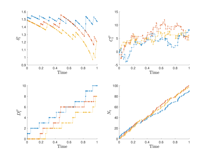
Refer to caption
Figure 2: Sample paths for the optimal discretion δsuperscript𝛿\delta^{*} (top left panel), number of missed trades Dδsuperscript𝐷superscript𝛿D^{\delta^{*}} (lower left panel), cost of strategy Cδsuperscript𝐶superscript𝛿C^{\delta^{*}} (top right panel), and number of trade attempts N𝑁N (lower right panel) for three simulations of the MPP. Parameters: α=0𝛼0\alpha=0, γ=0.07𝛾0.07\gamma=0.07, λ=100𝜆100\lambda=100, T=1𝑇1T=1.

Figure 3 reports various cost metrics of the optimal strategy for three values of the quadratic penalty parameter γ𝛾\gamma. The top panel shows histograms of the cost incurred by the strategy to fill trades, i.e., CTδsubscriptsuperscript𝐶superscript𝛿𝑇C^{\delta^{*}}_{T}, and the average cost of walking the LOB to fill trades, i.e., CTδ/(NTDTδ)subscriptsuperscript𝐶superscript𝛿𝑇subscript𝑁𝑇subscriptsuperscript𝐷superscript𝛿𝑇C^{\delta^{*}}_{T}/(N_{T}-D^{\delta^{*}}_{T}). Recall that the cost is negative (positive) when the trade is executed with price improvement (deterioration). The Figure shows that as the value of the quadratic penalty parameter increases: (i) the average cost of walking the book to fill trades increases, the total cost increases, and the average number of misses decreases, see bottom panels; (ii) the costs of walking the LOB increase because the strategy fills more orders (i.e., misses fewer trades), see the bottom-left panel. The bottom-right panel shows that the average ratio of missed trades to trade attempts decreases when the penalty for missing trades increases.
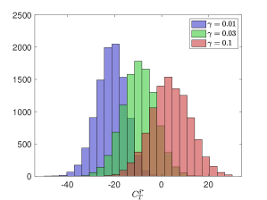
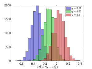
Refer to caption
Refer to caption
Refer to caption
Refer to caption
Figure 3: Top left panel: Histogram of the cost CTδsubscriptsuperscript𝐶superscript𝛿𝑇C^{\delta^{*}}_{T} of the strategy. Top right panel: Histogram of the extra cost per filled trade CTδ/(NTDTδ)subscriptsuperscript𝐶superscript𝛿𝑇subscript𝑁𝑇subscriptsuperscript𝐷superscript𝛿𝑇C^{\delta^{*}}_{T}/(N_{T}-D^{\delta^{*}}_{T}). Bottom left panel: Histogram of the number of misses DTδsubscriptsuperscript𝐷superscript𝛿𝑇D^{\delta^{*}}_{T}. Bottom right panel: Histogram of percentage of misses DTδ/NTsubscriptsuperscript𝐷superscript𝛿𝑇subscript𝑁𝑇D^{\delta^{*}}_{T}/N_{T}.

The tradeoff between higher fill ratios and costs of walking the book are clear. An agent who seeks very high fill ratios, i.e., high values of (NTDTδ)/NTsubscript𝑁𝑇superscriptsubscript𝐷𝑇superscript𝛿subscript𝑁𝑇(N_{T}-D_{T}^{\delta^{*}})/N_{T}, employs very high values of the penalty parameters in the performance criterion. Other agents may prefer to swap price improvements for price deteriorations in their overall trading strategy. For example, in the 10,000 simulations we discuss, when γ0.0693𝛾0.0693\gamma\approx 0.0693 the average cost of filled trades, CTδ/(NTDTδ)subscriptsuperscript𝐶superscript𝛿𝑇subscript𝑁𝑇subscriptsuperscript𝐷superscript𝛿𝑇C^{\delta^{*}}_{T}/(N_{T}-D^{\delta^{*}}_{T}), is zero and the average rate of missed trades, DTδ/NTsubscriptsuperscript𝐷superscript𝛿𝑇subscript𝑁𝑇D^{\delta^{*}}_{T}/N_{T} is 0.1048.

Finally, a naive strategy employed by liquidity takers is to send MLOs with no discretion to walk the LOB, see Cartea and Sánchez-Betancourt, (2018). Here, the expected ratio of missed trades to number of attempts and the expected cost of the strategy for an agent who sends all MLOs with no discretion to walk the LOB is 𝔼[DT0/NT]=0.5797𝔼delimited-[]subscriptsuperscript𝐷0𝑇subscript𝑁𝑇0.5797\mathbb{E}[D^{0}_{T}/N_{T}]=0.5797 and 𝔼[CT0]=29.25𝔼delimited-[]subscriptsuperscript𝐶0𝑇29.25\mathbb{E}[C^{0}_{T}]=-29.25, respectively. The expected cost is negative because the strategy does not accrue costs from walking the book, but may receive price improvements.

Optimal vs fixed discretion to walk the LOB

We compare the results of a strategy with α=0𝛼0\alpha=0 and γ>0𝛾0\gamma>0 with those of a fixed discretion latency-optimal strategy (i.e., α>0𝛼0\alpha>0 and γ=0𝛾0\gamma=0). Recall that when γ=0𝛾0\gamma=0 the optimal strategy is independent of the number of misses, so the agent sends all MLOs with discretion δ=αsuperscript𝛿𝛼\delta^{*}=\alpha, see (14).

The top panels in Figure 4 show the probability that the number of missed trades is less than 10% of trade attempts, i.e., [DTδ<0.1NT]delimited-[]subscriptsuperscript𝐷superscript𝛿𝑇0.1subscript𝑁𝑇\mathbb{P}[D^{\delta^{*}}_{T}<0.1\,N_{T}], and the expected cost of the strategy, i.e., 𝔼[CTδ]𝔼delimited-[]subscriptsuperscript𝐶superscript𝛿𝑇\mathbb{E}[C^{\delta^{*}}_{T}], when the agent sends orders with a fixed discretion to walk the LOB, i.e., γ=0𝛾0\gamma=0 and α[0, 2.5]𝛼02.5\alpha\in[0,\,2.5]. Similarly, the bottom panels show the probability that the number of missed trades is less than 10% of trade attempts, i.e., [DTδ<0.1NT]delimited-[]subscriptsuperscript𝐷superscript𝛿𝑇0.1subscript𝑁𝑇\mathbb{P}[D^{\delta^{*}}_{T}<0.1\,N_{T}] and the expected cost of the strategy, i.e., 𝔼[CTδ]𝔼delimited-[]subscriptsuperscript𝐶superscript𝛿𝑇\mathbb{E}[C^{\delta^{*}}_{T}] for γ[0.02, 0.16]𝛾0.020.16\gamma\in[0.02,\,0.16] and α=0𝛼0\alpha=0. The orange circle in each picture shows the lowest expected terminal cost 𝔼[CTδ]𝔼delimited-[]subscriptsuperscript𝐶superscript𝛿𝑇\mathbb{E}[C^{\delta^{*}}_{T}] for which [DTδ<0.1NT]0.95delimited-[]subscriptsuperscript𝐷superscript𝛿𝑇0.1subscript𝑁𝑇0.95\mathbb{P}[D^{\delta^{*}}_{T}<0.1\,N_{T}]\geq 0.95. The expected terminal cost of the fixed discretion latency-optimal strategy with α=1.91𝛼1.91\alpha=1.91 is approximately 9.52, and the expected cost obtained with the latency-optimal strategy, with γ=0.127𝛾0.127\gamma=0.127, is approximately 5.93.

Also, the expected number of misses when γ=0𝛾0\gamma=0 and α=1.9125𝛼1.9125\alpha=1.9125 (orange circle point in the top panels) is 𝔼[DTδ]=6.39𝔼delimited-[]subscriptsuperscript𝐷superscript𝛿𝑇6.39\mathbb{E}\left[D^{\delta^{*}}_{T}\right]=6.39, and when α=0𝛼0\alpha=0 and γ=0.1220𝛾0.1220\gamma=0.1220 (orange circle point in the bottom panels) we obtain 𝔼[DTδ]=5.41𝔼delimited-[]subscriptsuperscript𝐷superscript𝛿𝑇5.41\mathbb{E}\left[D^{\delta^{*}}_{T}\right]=5.41.

Thus, an agent who does not expect to miss more than 10% of the trades with high probability may prefer a latency-optimal optimal strategy with γ>0𝛾0\gamma>0 and α=0𝛼0\alpha=0 than a strategy that sends MLOs with a fixed discretion during the entire trading window.
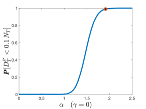
Refer to caption
Refer to caption
Refer to caption
Refer to caption
Figure 4: Top panel shows (DTδ<0.1NT)subscriptsuperscript𝐷superscript𝛿𝑇0.1subscript𝑁𝑇\mathbb{P}(D^{\delta^{*}}_{T}<0.1\,N_{T}) and 𝔼[CTδ]𝔼delimited-[]subscriptsuperscript𝐶superscript𝛿𝑇\mathbb{E}[C^{\delta^{*}}_{T}] when γ=0𝛾0\gamma=0 and for α[0,2.5]𝛼02.5\alpha\in[0,2.5], recall that δ=αsuperscript𝛿𝛼\delta^{*}=\alpha when γ=0𝛾0\gamma=0, see (14). Similarly, bottom panel shows (DTδ<0.1NT)subscriptsuperscript𝐷superscript𝛿𝑇0.1subscript𝑁𝑇\mathbb{P}(D^{\delta^{*}}_{T}<0.1\,N_{T}) and 𝔼[CTδ]𝔼delimited-[]subscriptsuperscript𝐶superscript𝛿𝑇\mathbb{E}[C^{\delta^{*}}_{T}] when α=0𝛼0\alpha=0 and γ[0.02,0.16]𝛾0.020.16\gamma\in[0.02,0.16]. In all pictures, the orange circle marks the lowest value of 𝔼[CT]𝔼delimited-[]subscript𝐶𝑇\mathbb{E}\left[C_{T}\right] when (DT<0.1NT)0.99subscript𝐷𝑇0.1subscript𝑁𝑇0.99\mathbb{P}\left(D_{T}<0.1\,N_{T}\right)\geq 0.99. Other model parameters: λ=100𝜆100\lambda=100, α=0𝛼0\alpha=0, and Z𝐍(0.2,1)similar-to𝑍𝐍0.21Z\sim\mathbf{N}(0.2,1) for all trades.

Pinned arrival rates

In this section, we assume the arrival intensity of the agent’s MLOs is

λt=MNtTt+ϵ,subscriptsuperscript𝜆𝑡𝑀subscript𝑁superscript𝑡𝑇𝑡italic-ϵ\lambda^{\star}_{t}=\frac{M-N_{t^{-}}}{T-t+\epsilon}\,, (31)

where M>0𝑀0M>0 is a positive integer, ϵ>0italic-ϵ0\epsilon>0 and recall that Ntsubscript𝑁𝑡N_{t} denotes the number of trade attempts. The intensity λtsubscriptsuperscript𝜆𝑡\lambda^{\star}_{t} is bounded by λ¯=M/ϵ¯𝜆𝑀italic-ϵ\bar{\lambda}=M/\epsilon, which is a condition we require in the latency-optimal strategy we derived above, and if ϵ=0italic-ϵ0\epsilon=0, the intensity guarantees that NT=Msubscript𝑁𝑇𝑀N_{T}=M, see Conforti, (2016) and Hoyle, (2010).

Now, use the Markov property of δsuperscript𝛿\delta^{*} to write δ=h(t,Dt,Nt)superscript𝛿𝑡subscript𝐷superscript𝑡subscript𝑁superscript𝑡\delta^{*}=h(t,D_{t^{-}},N_{t^{-}}), where the function hh satisfies the PIDE

0=th(t,D,N)0subscript𝑡𝑡𝐷𝑁\displaystyle 0=\partial_{t}h(t,D,N) +(h(t,D,N)MNTt+ϵϕt(z)dz)(h(t,D+1,N+1)h(t,D,N))superscriptsubscript𝑡𝐷𝑁𝑀𝑁𝑇𝑡italic-ϵsubscriptitalic-ϕ𝑡𝑧differential-d𝑧𝑡𝐷1𝑁1𝑡𝐷𝑁\displaystyle+\left(\int_{h(t,D,N)}^{\infty}\frac{M-N}{T-t+\epsilon}\,\phi_{t}(z)\,\mathrm{d}z\right)\,\left(h(t,D+1,N+1)-h(t,D,N)\right)
+(h(t,D,N)MNTt+ϵϕt(z)dz)(h(t,D,N+1)h(t,D,N)),superscriptsubscript𝑡𝐷𝑁𝑀𝑁𝑇𝑡italic-ϵsubscriptitalic-ϕ𝑡𝑧differential-d𝑧𝑡𝐷𝑁1𝑡𝐷𝑁\displaystyle+\left(\int_{-\infty}^{h(t,D,N)}\,\frac{M-N}{T-t+\epsilon}\,\phi_{t}(z)\,\mathrm{d}z\right)\,\left(h(t,D,N+1)-h(t,D,N)\right)\,,

with

h(t,D,M)=2γD+γ+αandh(T,D,N)=2γD+γ+α.formulae-sequence𝑡𝐷𝑀2𝛾𝐷𝛾𝛼and𝑇𝐷𝑁2𝛾𝐷𝛾𝛼\displaystyle h(t,D,M)=2\,\gamma\,D+\gamma+\alpha\qquad\text{and}\qquad h(T,D,N)=2\,\gamma\,D+\gamma+\alpha\,.

Figure 5 shows the optimal discretion to walk the LOB for various values of missed trades and target number of trades M=100𝑀100M=100. The interpretation is similar to that of Figure 1.
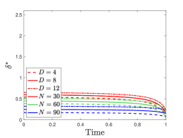
Refer to caption
Refer to caption
Refer to caption
Figure 5: Optimal strategy δsuperscript𝛿\delta^{*} for various values of γ𝛾\gamma, number of misses, and number of attempts. From left to right, penalty parameter is γ=0.01𝛾0.01\gamma=0.01, γ=0.03𝛾0.03\gamma=0.03, and γ=0.1𝛾0.1\gamma=0.1. Dotted line Nt=30subscript𝑁𝑡30N_{t}=30, solid line Nt=60subscript𝑁𝑡60N_{t}=60, and dot-dash line Nt=90subscript𝑁𝑡90N_{t}=90. Blue lines Dtδ=4superscriptsubscript𝐷𝑡superscript𝛿4D_{t}^{\delta^{*}}=4, green lines Dtδ=8superscriptsubscript𝐷𝑡superscript𝛿8D_{t}^{\delta^{*}}=8, red lines Dtδ=12superscriptsubscript𝐷𝑡superscript𝛿12D_{t}^{\delta^{*}}=12. The remaining parameters are: M=100𝑀100M=100, α=0𝛼0\alpha=0, ϵ=0.1italic-ϵ0.1\epsilon=0.1, Z𝐍(0.2,1)similar-to𝑍𝐍0.21Z\sim\mathbf{N}(0.2,1).

We perform 10,000 simulations with the same parameters as above and use the arrival rate of the MLOs as in (31) with ϵ=0.1italic-ϵ0.1\epsilon=0.1. Figures 6 and 7 report the results, which have a similar interpretation to that of Figures 2 and 3, respectively.
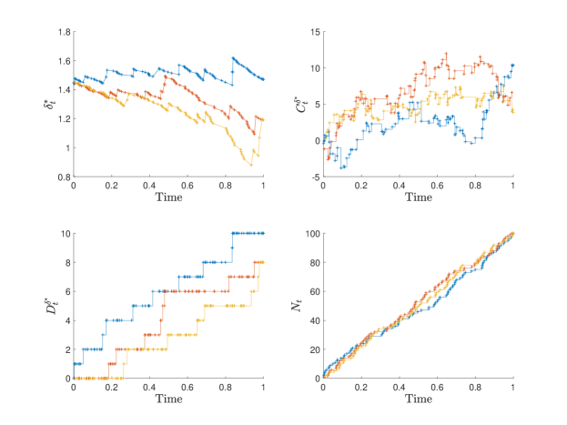
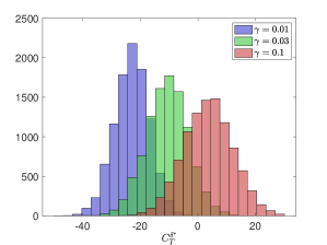
Refer to caption
Figure 6: Sample paths for the optimal discretion δsuperscript𝛿\delta^{*} (top left panel), number of missed trades Dδsuperscript𝐷superscript𝛿D^{\delta^{*}} (lower left panel), cost of strategy Cδsuperscript𝐶superscript𝛿C^{\delta^{*}} (top right panel), and number of trade attempts N𝑁N (lower right panel) for three simulations of the MPP. Parameters: α=0𝛼0\alpha=0, γ=0.07𝛾0.07\gamma=0.07, ϵ=0.1italic-ϵ0.1\epsilon=0.1, M=100𝑀100M=100, T=1𝑇1T=1.
Refer to caption
Refer to caption
Refer to caption
Refer to caption
Figure 7: Top left panel: Histogram of the cost CTδsubscriptsuperscript𝐶superscript𝛿𝑇C^{\delta^{*}}_{T} of the strategy. Top right panel: Histogram of the extra cost per filled trade CTδ/(NTDTδ)subscriptsuperscript𝐶superscript𝛿𝑇subscript𝑁𝑇subscriptsuperscript𝐷superscript𝛿𝑇C^{\delta^{*}}_{T}/(N_{T}-D^{\delta^{*}}_{T}). Bottom left panel: Histogram of the number of misses DTδsubscriptsuperscript𝐷superscript𝛿𝑇D^{\delta^{*}}_{T}. Bottom right panel: Histogram of percentage of misses DTδ/NTsubscriptsuperscript𝐷superscript𝛿𝑇subscript𝑁𝑇D^{\delta^{*}}_{T}/N_{T}.

Conclusions

With few exceptions, the literature on algorithmic trading assumes that latency in the marketplace is zero. This is not accurate, and the effects of latency on the efficacy of liquidity making and taking strategies are economically significant. In this paper we proposed a model to improve the marksmanship of the orders sent by liquidity takers when, due to latency, the limit order book is a moving target.

We showed how a liquidity taker chooses the price limit of marketable orders when there is latency in the marketplace. The optimal strategy balances the tradeoff between the costs of walking the book and the number of missed trades over a trading horizon. We modelled the effects of latency as a marked point process that captures the interaction between liquidity taking orders and the limit orders resting in the book. We characterized the optimal price limit of marketable orders as a solution to a FBSDE, which, to the best of our knowledge, is new and, as the extant literature does not have uniqueness and existence results, we prove both.

The strategy developed here may be implemented as another layer of any liquidity taking strategy (especially those that follow a stochastic trading schedule) that incorrectly assumes zero latency. Our framework can be applied in other contexts too. In its most general form, we solve a problem in which the agent decides how much she is willing to pay to absorb a stochastic shock to achieve an objective or complete a task. For example, market makers in foreign exchange markets with ‘last look’ can employ the framework developed in this paper. The last look feature allows liquidity makers to reject trades, so they are not picked off by faster liquidity taking traders, see Oomen, (2017) and Cartea et al., (2018). Specifically, with our framework, a foreign exchange market maker can obtain the optimal tolerance that maximizes the number of incoming marketable orders she is willing to fill while minimizing losses to the fast traders who snipe her stale quotes in the LOB.

References

  • Almgren, (2012) Almgren, R. (2012). Optimal trading with stochastic liquidity and volatility. SIAM Journal on Financial Mathematics, 3(1):163–181.
  • Antonelli, (1993) Antonelli, F. (1993). Backward-forward stochastic differential equations. The Annals of Applied Probability, 3(3):777–793.
  • Bandini, (2016) Bandini, E. (2016). Probabilistic representation of HJB equations for optimal control of jump processes, BSDEs and related stochastic calculus. PhD Thesis.
  • Barger and Lorig, (2019) Barger, W. and Lorig, M. (2019). Optimal liquidation under stochastic price impact. International Journal of Theoretical and Applied Finance, 22(02):1850059.
  • Cartea et al., (2018) Cartea, Á., Jaimungal, S., and Walton, J. (2018). Foreign exchange markets with Last Look. Mathematics and Financial Economics (forthcoming).
  • Cartea and Sánchez-Betancourt, (2018) Cartea, Á. and Sánchez-Betancourt, L. (2018). The shadow price of latency: Improving intraday fill ratios in foreign exchange markets. Available at SSRN 3190961.
  • (7) Casgrain, P. and Jaimungal, S. (2018a). Mean-field games with differing beliefs for algorithmic trading. arXiv preprint arXiv:1810.06101.
  • (8) Casgrain, P. and Jaimungal, S. (2018b). Mean-field games with partial information for algorithmic trading. arXiv preprint arXiv:1803.04094.
  • Cohen and Elliott, (2015) Cohen, S. N. and Elliott, R. J. (2015). Stochastic calculus and applications, volume 2. Springer.
  • Conforti, (2016) Conforti, G. (2016). Bridges of Markov counting processes: quantitative estimates. Electronic Communications in Probability, 21.
  • Confortola and Fuhrman, (2013) Confortola, F. and Fuhrman, M. (2013). Backward stochastic differential equations and optimal control of marked point processes. SIAM Journal on Control and Optimization, 51(5):3592–3623.
  • Confortola et al., (2016) Confortola, F., Fuhrman, M., and Jacod, J. (2016). Backward stochastic differential equation driven by a marked point process: An elementary approach with an application to optimal control. The Annals of Applied Probability, 26(3):1743–1773.
  • Duffie and Epstein, (1992) Duffie, D. and Epstein, L. G. (1992). Stochastic differential utility. Econometrica: Journal of the Econometric Society, pages 353–394.
  • Gao and Wang, (2018) Gao, X. and Wang, Y. (2018). Electronic market making and latency. arXiv preprint arXiv:1806.05849.
  • Guéant, (2016) Guéant, O. (2016). The financial mathematics of market liquidity: From optimal execution to market making, volume 33. CRC Press.
  • Hoyle, (2010) Hoyle, E. (2010). Information-based models for finance and insurance. PhD Thesis.
  • Jeanblanc et al., (2009) Jeanblanc, M., Yor, M., and Chesney, M. (2009). Mathematical methods for financial markets. Springer Science & Business Media.
  • Jianming, (2000) Jianming, X. (2000). Backward stochastic differential equation with random measures. Acta Mathematicae Applicatae Sinica, 16(3):225–234.
  • Lehalle and Laruelle, (2013) Lehalle, C.-A. and Laruelle, S. (2013). Market Microstructure in Practice. World Scientific.
  • Lehalle and Mounjid, (2017) Lehalle, C.-A. and Mounjid, O. (2017). Limit order strategic placement with adverse selection risk and the role of latency. Market Microstructure and Liquidity, 03(01):1750009.
  • Moallemi and Saĝlam, (2013) Moallemi, C. C. and Saĝlam, M. (2013). The cost of latency in high-frequency trading. Operations Research, 61(5):1070–1086.
  • Oomen, (2017) Oomen, R. (2017). Last Look. Quantitative Finance, 17:1057–1070.
  • Peng and Wu, (1999) Peng, S. and Wu, Z. (1999). Fully coupled forward-backward stochastic differential equations and applications to optimal control. SIAM Journal on Control and Optimization, 37(3):825–843.
  • Stoikov and Waeber, (2016) Stoikov, S. and Waeber, R. (2016). Reducing transaction costs with low-latency trading algorithms. Quantitative Finance, 16(9):1445–1451.
  • Zhen, (1999) Zhen, W. (1999). Forward-backward stochastic differential equations with brownian motion and poisson process. Acta Mathematicae Applicatae Sinica, 15(4):433–443.

Appendix A Proof of Lemma 1

We prove the lemma in three parts. First we work out the Gâteaux derivative of the cost function. We use (8) to write

1ϵ{𝔼[CTδ+ϵw]𝔼[CTδ]}1italic-ϵ𝔼delimited-[]subscriptsuperscript𝐶𝛿italic-ϵ𝑤𝑇𝔼delimited-[]subscriptsuperscript𝐶𝛿𝑇\displaystyle\frac{1}{\epsilon}\,\left\{\mathbb{E}\left[C^{\delta+\epsilon\,w}_{T}\right]-\mathbb{E}\left[C^{\delta}_{T}\right]\right\} =1ϵ{𝔼[0Tz(G^(δt+ϵwtz)G^(δtz))ϕt(dz)dAt]}absent1italic-ϵ𝔼delimited-[]superscriptsubscript0𝑇subscript𝑧^𝐺subscript𝛿𝑡italic-ϵsubscript𝑤𝑡𝑧^𝐺subscript𝛿𝑡𝑧subscriptitalic-ϕ𝑡d𝑧differential-dsubscript𝐴𝑡\displaystyle=\frac{1}{\epsilon}\,\left\{\mathbb{E}\left[\int_{0}^{T}\int_{\mathbb{R}}z\,\left({\hat{G}}(\delta_{t}+\epsilon\,w_{t}-z)-{\hat{G}}(\delta_{t}-z)\right)\,\phi_{t}(\mathrm{d}z)\,\mathrm{d}A_{t}\right]\right\}
=1ϵ{𝔼[0Tδtδt+ϵwtzϕt(dz)dAt]}absent1italic-ϵ𝔼delimited-[]superscriptsubscript0𝑇superscriptsubscriptsubscript𝛿𝑡subscript𝛿𝑡italic-ϵsubscript𝑤𝑡𝑧subscriptitalic-ϕ𝑡d𝑧differential-dsubscript𝐴𝑡\displaystyle=\frac{1}{\epsilon}\,\left\{\mathbb{E}\left[\int_{0}^{T}\int_{\delta_{t}}^{\delta_{t}+\epsilon\,w_{t}}z\,\phi_{t}(\mathrm{d}z)\,\mathrm{d}A_{t}\right]\right\}
=𝔼[0T1ϵ{δtδt+ϵwtzϕt(dz)}dAt].absent𝔼delimited-[]superscriptsubscript0𝑇1italic-ϵsuperscriptsubscriptsubscript𝛿𝑡subscript𝛿𝑡italic-ϵsubscript𝑤𝑡𝑧subscriptitalic-ϕ𝑡d𝑧differential-dsubscript𝐴𝑡\displaystyle=\mathbb{E}\left[\int_{0}^{T}\frac{1}{\epsilon}\left\{\int_{\delta_{t}}^{\delta_{t}+\epsilon\,w_{t}}z\,\phi_{t}(\mathrm{d}z)\right\}\,\mathrm{d}A_{t}\right]\,.

Then, by the dominated convergence theorem and the fundamental theorem of calculus, we have

𝒟JC(δ),w𝒟superscript𝐽C𝛿𝑤\displaystyle\langle\mathcal{D}\,J^{\text{C}}(\delta),w\rangle =limϵ0JC(δ+ϵw)JC(δ)ϵabsentsubscriptitalic-ϵ0superscript𝐽C𝛿italic-ϵ𝑤superscript𝐽C𝛿italic-ϵ\displaystyle=\lim_{\epsilon\to 0}\frac{J^{\text{C}}(\delta+\epsilon\,w)-J^{\text{C}}(\delta)}{\epsilon}
=limϵ01ϵ{𝔼[CTδ+ϵw]𝔼[CTδ]}=𝔼[0Tδtwtϕt(δt)dAt].absentsubscriptitalic-ϵ01italic-ϵ𝔼delimited-[]subscriptsuperscript𝐶𝛿italic-ϵ𝑤𝑇𝔼delimited-[]subscriptsuperscript𝐶𝛿𝑇𝔼delimited-[]superscriptsubscript0𝑇subscript𝛿𝑡subscript𝑤𝑡subscriptitalic-ϕ𝑡subscript𝛿𝑡differential-dsubscript𝐴𝑡\displaystyle=\lim_{\epsilon\to 0}\frac{1}{\epsilon}\,\left\{\mathbb{E}\left[C^{\delta+\epsilon\,w}_{T}\right]-\mathbb{E}\left[C^{\delta}_{T}\right]\right\}=\mathbb{E}\left[\int_{0}^{T}\delta_{t}\,w_{t}\,\phi_{t}(\delta_{t})\,\mathrm{d}A_{t}\right]\,.

Next we work out the Gâteaux derivative of the linear penalty. Note that

1ϵ{𝔼[DTδ+ϵw]𝔼[DTδ]}1italic-ϵ𝔼delimited-[]subscriptsuperscript𝐷𝛿italic-ϵ𝑤𝑇𝔼delimited-[]subscriptsuperscript𝐷𝛿𝑇\displaystyle\frac{1}{\epsilon}\,\left\{\mathbb{E}\left[D^{\delta+\epsilon\,w}_{T}\right]-\mathbb{E}\left[D^{\delta}_{T}\right]\right\} =1ϵ{𝔼[0T(G(δt+ϵwtz)G(δtz))p~(dz,dt)]}absent1italic-ϵ𝔼delimited-[]superscriptsubscript0𝑇subscript𝐺subscript𝛿𝑡italic-ϵsubscript𝑤𝑡𝑧𝐺subscript𝛿𝑡𝑧~𝑝d𝑧d𝑡\displaystyle=\frac{1}{\epsilon}\,\left\{\mathbb{E}\left[\int_{0}^{T}\int_{\mathbb{R}}\left(G(\delta_{t}+\epsilon\,w_{t}-z)-G(\delta_{t}-z)\right)\,\tilde{p}(\mathrm{d}z,\,\mathrm{d}t)\right]\right\}
=𝔼[0T1ϵ{δt+ϵwtδtϕt(dz)}dAt],absent𝔼delimited-[]superscriptsubscript0𝑇1italic-ϵsubscriptsuperscriptsubscript𝛿𝑡subscript𝛿𝑡italic-ϵsubscript𝑤𝑡subscriptitalic-ϕ𝑡d𝑧differential-dsubscript𝐴𝑡\displaystyle=\mathbb{E}\left[\int_{0}^{T}\frac{1}{\epsilon}\,\left\{\int^{\delta_{t}}_{\delta_{t}+\epsilon\,w_{t}}\phi_{t}(\mathrm{d}z)\right\}\,\mathrm{d}A_{t}\right]\,,

therefore, we have

limϵ01ϵ{𝔼[DTδ+ϵw]𝔼[DTδ]}subscriptitalic-ϵ01italic-ϵ𝔼delimited-[]subscriptsuperscript𝐷𝛿italic-ϵ𝑤𝑇𝔼delimited-[]subscriptsuperscript𝐷𝛿𝑇\displaystyle\lim_{\epsilon\to 0}\frac{1}{\epsilon}\,\bigg{\{}\mathbb{E}\left[D^{\delta+\epsilon\,w}_{T}\right]-\mathbb{E}\left[D^{\delta}_{T}\right]\bigg{\}} =𝔼[0Twtϕt(δt)dAt].absent𝔼delimited-[]superscriptsubscript0𝑇subscript𝑤𝑡subscriptitalic-ϕ𝑡subscript𝛿𝑡differential-dsubscript𝐴𝑡\displaystyle=-\mathbb{E}\left[\int_{0}^{T}w_{t}\,\phi_{t}(\delta_{t})\,\mathrm{d}A_{t}\right]\,.

Finally, we work out the Gâteaux derivative of the quadratic penalty. We write

1ϵ{𝔼[(DTδ+ϵw)2]𝔼[(DTδ)2]}1italic-ϵ𝔼delimited-[]superscriptsubscriptsuperscript𝐷𝛿italic-ϵ𝑤𝑇2𝔼delimited-[]superscriptsubscriptsuperscript𝐷𝛿𝑇2\displaystyle\frac{1}{\epsilon}\,\Bigg{\{}\mathbb{E}\left[\left(D^{\delta+\epsilon\,w}_{T}\right)^{2}\right]-\mathbb{E}\left[\left(D^{\delta}_{T}\right)^{2}\right]\Bigg{\}} =2ϵ{𝔼[0TDtδ+ϵwG(δt+ϵwtz)p~(dz,dt)]\displaystyle=\frac{2}{\epsilon}\,\Bigg{\{}\mathbb{E}\left[\int_{0}^{T}\int_{\mathbb{R}}D^{\delta+\epsilon\,w}_{t^{-}}\,G(\delta_{t}+\epsilon\,w_{t}-z)\,\tilde{p}(\mathrm{d}z,\,\mathrm{d}t)\right]
𝔼[0TDtδG(δtz)p~(dz,dt)]}\displaystyle\quad\quad\quad-\mathbb{E}\left[\int_{0}^{T}\int_{\mathbb{R}}D^{\delta}_{t^{-}}\,G(\delta_{t}-z)\,\tilde{p}(\mathrm{d}z,\,\mathrm{d}t)\right]\Bigg{\}}
+1ϵ{𝔼[0TG(δt+ϵwtz)G(δtz)p~(dz,dt)]}.1italic-ϵ𝔼delimited-[]superscriptsubscript0𝑇subscript𝐺subscript𝛿𝑡italic-ϵsubscript𝑤𝑡𝑧𝐺subscript𝛿𝑡𝑧~𝑝d𝑧d𝑡\displaystyle\quad+\frac{1}{\epsilon}\,\Bigg{\{}\mathbb{E}\left[\int_{0}^{T}\int_{\mathbb{R}}G(\delta_{t}+\epsilon\,w_{t}-z)-G(\delta_{t}-z)\,\tilde{p}(\mathrm{d}z,\,\mathrm{d}t)\right]\Bigg{\}}\,.

Subtract and add

2ϵ{𝔼[0TDtδ+ϵwG(δtz)p~(dz,dt)]}2italic-ϵ𝔼delimited-[]superscriptsubscript0𝑇subscriptsubscriptsuperscript𝐷𝛿italic-ϵ𝑤superscript𝑡𝐺subscript𝛿𝑡𝑧~𝑝d𝑧d𝑡\frac{2}{\epsilon}\,\bigg{\{}\mathbb{E}\left[\int_{0}^{T}\int_{\mathbb{R}}D^{\delta+\epsilon\,w}_{t^{-}}\,G(\delta_{t}-z)\,\tilde{p}(\mathrm{d}z,\,\mathrm{d}t)\right]\bigg{\}}

to the right-hand side of the equation above and write

1ϵ{𝔼[(DTδ+ϵw)2]𝔼[(DTδ)2]}1italic-ϵ𝔼delimited-[]superscriptsubscriptsuperscript𝐷𝛿italic-ϵ𝑤𝑇2𝔼delimited-[]superscriptsubscriptsuperscript𝐷𝛿𝑇2\displaystyle\frac{1}{\epsilon}\,\Bigg{\{}\mathbb{E}\left[\left(D^{\delta+\epsilon\,w}_{T}\right)^{2}\right]-\mathbb{E}\left[\left(D^{\delta}_{T}\right)^{2}\right]\Bigg{\}}
=2ϵ{𝔼[0T(Dtδ+ϵwG(δt+ϵwtz)Dtδ+ϵwG(δtz))p~(dz,dt)]\displaystyle\quad=\frac{2}{\epsilon}\,\Bigg{\{}\mathbb{E}\left[\int_{0}^{T}\int_{\mathbb{R}}\left(D^{\delta+\epsilon\,w}_{t^{-}}\,G(\delta_{t}+\epsilon\,w_{t}-z)-D^{\delta+\epsilon\,w}_{t^{-}}\,G(\delta_{t}-z)\right)\,\tilde{p}(\mathrm{d}z,\,\mathrm{d}t)\right]
+𝔼[0T(Dtδ+ϵwG(δtz)DtδG(δtz))p~(dz,dt)]}\displaystyle\quad\quad\quad\quad+\mathbb{E}\left[\int_{0}^{T}\int_{\mathbb{R}}\left(D^{\delta+\epsilon\,w}_{t^{-}}\,G(\delta_{t}-z)-D^{\delta}_{t^{-}}\,G(\delta_{t}-z)\right)\,\tilde{p}(\mathrm{d}z,\,\mathrm{d}t)\right]\Bigg{\}}
+1ϵ{𝔼[0T(G(δt+ϵwtz)G(δtz))p~(dz,dt)]}1italic-ϵ𝔼delimited-[]superscriptsubscript0𝑇subscript𝐺subscript𝛿𝑡italic-ϵsubscript𝑤𝑡𝑧𝐺subscript𝛿𝑡𝑧~𝑝d𝑧d𝑡\displaystyle\quad\quad+\frac{1}{\epsilon}\,\Bigg{\{}\mathbb{E}\left[\int_{0}^{T}\int_{\mathbb{R}}\left(G(\delta_{t}+\epsilon\,w_{t}-z)-G(\delta_{t}-z)\right)\,\tilde{p}(\mathrm{d}z,\,\mathrm{d}t)\right]\Bigg{\}}
=2{𝔼[0T(Dtδ+ϵwG(δt+ϵwtz)G(δtz)ϵ)p~(dz,dt)]\displaystyle\quad=2\,\Bigg{\{}{\mathbb{E}\left[\int_{0}^{T}\int_{\mathbb{R}}\left(D^{\delta+\epsilon\,w}_{t^{-}}\,\frac{G(\delta_{t}+\epsilon\,w_{t}-z)-G(\delta_{t}-z)}{\epsilon}\right)\,\tilde{p}(\mathrm{d}z,\,\mathrm{d}t)\right]} (QP1)
+𝔼[0T(Dtδ+ϵwDtδϵG(δtz))p~(dz,dt)]}\displaystyle\quad\quad\quad\quad+{\mathbb{E}\left[\int_{0}^{T}\int_{\mathbb{R}}\left(\frac{D^{\delta+\epsilon\,w}_{t^{-}}-D^{\delta}_{t^{-}}}{\epsilon}\,G(\delta_{t}-z)\right)\,\tilde{p}(\mathrm{d}z,\,\mathrm{d}t)\right]}\Bigg{\}} (QP2)
+𝔼[0T(G(δt+ϵwtz)G(δtz)ϵ)p~(dz,dt)].𝔼delimited-[]superscriptsubscript0𝑇subscript𝐺subscript𝛿𝑡italic-ϵsubscript𝑤𝑡𝑧𝐺subscript𝛿𝑡𝑧italic-ϵ~𝑝d𝑧d𝑡\displaystyle\quad\quad+{\mathbb{E}\left[\int_{0}^{T}\int_{\mathbb{R}}\left(\frac{G(\delta_{t}+\epsilon\,w_{t}-z)-G(\delta_{t}-z)}{\epsilon}\right)\,\tilde{p}(\mathrm{d}z,\,\mathrm{d}t)\right]}\,. (QP3)

Next, take the limit of QP1, QP2, and QP3 as ϵitalic-ϵ\epsilon approaches zero. The limit of QP1 is given by

limϵ0QP1subscriptitalic-ϵ0QP1\displaystyle\lim_{\epsilon\to 0}\text{QP1} =limϵ0𝔼[0TDtδ+ϵwG(δt+ϵwtz)G(δtz)ϵp~(dz,dt)]absentsubscriptitalic-ϵ0𝔼delimited-[]superscriptsubscript0𝑇subscriptsubscriptsuperscript𝐷𝛿italic-ϵ𝑤superscript𝑡𝐺subscript𝛿𝑡italic-ϵsubscript𝑤𝑡𝑧𝐺subscript𝛿𝑡𝑧italic-ϵ~𝑝d𝑧d𝑡\displaystyle=\lim_{\epsilon\to 0}\mathbb{E}\left[\int_{0}^{T}\int_{\mathbb{R}}D^{\delta+\epsilon\,w}_{t^{-}}\,\frac{G(\delta_{t}+\epsilon\,w_{t}-z)-G(\delta_{t}-z)}{\epsilon}\,\tilde{p}(\mathrm{d}z,\,\mathrm{d}t)\right]
=limϵ0𝔼[0TDtδ+ϵw1ϵ{δt+ϵwtδtϕt(dz)}dAt]absentsubscriptitalic-ϵ0𝔼delimited-[]superscriptsubscript0𝑇subscriptsuperscript𝐷𝛿italic-ϵ𝑤superscript𝑡1italic-ϵsuperscriptsubscriptsubscript𝛿𝑡italic-ϵsubscript𝑤𝑡subscript𝛿𝑡subscriptitalic-ϕ𝑡d𝑧differential-dsubscript𝐴𝑡\displaystyle=\lim_{\epsilon\to 0}\mathbb{E}\left[\int_{0}^{T}\,D^{\delta+\epsilon\,w}_{t^{-}}\,\frac{1}{\epsilon}\,\left\{\int_{\delta_{t}+\epsilon\,w_{t}}^{\delta_{t}}\phi_{t}(\mathrm{d}z)\,\right\}\mathrm{d}A_{t}\right]
=𝔼[0TDtδwtϕt(δt)dAt].absent𝔼delimited-[]superscriptsubscript0𝑇subscriptsuperscript𝐷𝛿superscript𝑡subscript𝑤𝑡subscriptitalic-ϕ𝑡subscript𝛿𝑡differential-dsubscript𝐴𝑡\displaystyle=-\mathbb{E}\left[\int_{0}^{T}D^{\delta}_{t^{-}}\,w_{t}\,\phi_{t}(\delta_{t})\,\mathrm{d}A_{t}\right]\,.

The last equality follows from the dominated convergence theorem and because limϵ0Dtδ+ϵw=Dtδsubscriptitalic-ϵ0subscriptsuperscript𝐷𝛿italic-ϵ𝑤superscript𝑡subscriptsuperscript𝐷𝛿superscript𝑡\lim_{\epsilon\to 0}D^{\delta+\epsilon\,w}_{t^{-}}=D^{\delta}_{t^{-}} almost surely.

The limit of QP2 is given by

limϵ0QP2subscriptitalic-ϵ0QP2\displaystyle\lim_{\epsilon\to 0}\text{QP2}
=limϵ0𝔼[0TDtδ+ϵwDtδϵG(δtz)p~(dz,dt)]absentsubscriptitalic-ϵ0𝔼delimited-[]superscriptsubscript0𝑇subscriptsubscriptsuperscript𝐷𝛿italic-ϵ𝑤superscript𝑡subscriptsuperscript𝐷𝛿superscript𝑡italic-ϵ𝐺subscript𝛿𝑡𝑧~𝑝d𝑧d𝑡\displaystyle\quad=\lim_{\epsilon\to 0}\mathbb{E}\left[\int_{0}^{T}\int_{\mathbb{R}}\frac{D^{\delta+\epsilon\,w}_{t^{-}}-D^{\delta}_{t^{-}}}{\epsilon}\,G(\delta_{t}-z)\,\tilde{p}(\mathrm{d}z,\,\mathrm{d}t)\right]
=limϵ0𝔼[0TG(δtz)(0tG(δs+ϵwsz)G(δsz)ϵp(dz,ds))p~(dz,dt)]absentsubscriptitalic-ϵ0𝔼delimited-[]superscriptsubscript0𝑇subscript𝐺subscript𝛿𝑡𝑧superscriptsubscript0superscript𝑡subscript𝐺subscript𝛿𝑠italic-ϵsubscript𝑤𝑠superscript𝑧𝐺subscript𝛿𝑠superscript𝑧italic-ϵ𝑝dsuperscript𝑧d𝑠~𝑝d𝑧d𝑡\displaystyle\quad=\lim_{\epsilon\to 0}\mathbb{E}\left[\int_{0}^{T}\int_{\mathbb{R}}G(\delta_{t}-z)\,\left(\int_{0}^{t^{-}}\int_{\mathbb{R}}\frac{G(\delta_{s}+\epsilon\,w_{s}-z^{\prime})-G(\delta_{s}-z^{\prime})}{\epsilon}\,p(\mathrm{d}z^{\prime},\,\mathrm{d}s)\right)\,\tilde{p}(\mathrm{d}z,\,\mathrm{d}t)\right]
=limϵ0𝔼[0TG(δt+ϵwtz)G(δtz)ϵ(tTG(δsz)p~(dz,ds))p(dz,dt)]absentsubscriptitalic-ϵ0𝔼delimited-[]superscriptsubscript0𝑇subscript𝐺subscript𝛿𝑡italic-ϵsubscript𝑤𝑡𝑧𝐺subscript𝛿𝑡𝑧italic-ϵsuperscriptsubscript𝑡𝑇subscript𝐺subscript𝛿𝑠𝑧~𝑝dsuperscript𝑧d𝑠𝑝d𝑧d𝑡\displaystyle\quad=\lim_{\epsilon\to 0}\mathbb{E}\left[\int_{0}^{T}\int_{\mathbb{R}}\frac{G(\delta_{t}+\epsilon\,w_{t}-z)-G(\delta_{t}-z)}{\epsilon}\,\left(\int_{t}^{T}\int_{\mathbb{R}}G(\delta_{s}-z)\,\tilde{p}(\mathrm{d}z^{\prime},\,\mathrm{d}s)\right)\,p(\mathrm{d}z,\,\mathrm{d}t)\right]
=limϵ0𝔼[0TG(δt+ϵwtz)G(δtz)ϵ𝔼t[tTG(δsz)p~(dz,ds)]p(dz,dt)]absentsubscriptitalic-ϵ0𝔼delimited-[]superscriptsubscript0𝑇subscript𝐺subscript𝛿𝑡italic-ϵsubscript𝑤𝑡𝑧𝐺subscript𝛿𝑡𝑧italic-ϵsubscript𝔼superscript𝑡delimited-[]superscriptsubscript𝑡𝑇subscript𝐺subscript𝛿𝑠𝑧~𝑝dsuperscript𝑧d𝑠𝑝d𝑧d𝑡\displaystyle\quad=\lim_{\epsilon\to 0}\mathbb{E}\left[\int_{0}^{T}\int_{\mathbb{R}}\frac{G(\delta_{t}+\epsilon\,w_{t}-z)-G(\delta_{t}-z)}{\epsilon}\,\mathbb{E}_{t^{-}}\left[\int_{t}^{T}\int_{\mathbb{R}}G(\delta_{s}-z)\,\tilde{p}(\mathrm{d}z^{\prime},\,\mathrm{d}s)\right]\,p(\mathrm{d}z,\,\mathrm{d}t)\right]
=limϵ0𝔼[0TG(δt+ϵwtz)G(δtz)ϵ𝔼t[tTG(δsz)p~(dz,ds)]p~(dz,dt)]absentsubscriptitalic-ϵ0𝔼delimited-[]superscriptsubscript0𝑇subscript𝐺subscript𝛿𝑡italic-ϵsubscript𝑤𝑡𝑧𝐺subscript𝛿𝑡𝑧italic-ϵsubscript𝔼superscript𝑡delimited-[]superscriptsubscript𝑡𝑇subscript𝐺subscript𝛿𝑠𝑧~𝑝dsuperscript𝑧d𝑠~𝑝d𝑧d𝑡\displaystyle\quad=\lim_{\epsilon\to 0}\mathbb{E}\left[\int_{0}^{T}\int_{\mathbb{R}}\frac{G(\delta_{t}+\epsilon\,w_{t}-z)-G(\delta_{t}-z)}{\epsilon}\,\mathbb{E}_{t^{-}}\left[\int_{t}^{T}\int_{\mathbb{R}}G(\delta_{s}-z)\,\tilde{p}(\mathrm{d}z^{\prime},\,\mathrm{d}s)\right]\,\tilde{p}(\mathrm{d}z,\,\mathrm{d}t)\right]
=limϵ0𝔼[0T1ϵδt+ϵwtδtϕt(dz)𝔼t[tTG(δsz)p~(dz,ds)]dAt]absentsubscriptitalic-ϵ0𝔼delimited-[]superscriptsubscript0𝑇1italic-ϵsuperscriptsubscriptsubscript𝛿𝑡italic-ϵsubscript𝑤𝑡subscript𝛿𝑡subscriptitalic-ϕ𝑡d𝑧subscript𝔼superscript𝑡delimited-[]superscriptsubscript𝑡𝑇subscript𝐺subscript𝛿𝑠𝑧~𝑝dsuperscript𝑧d𝑠differential-dsubscript𝐴𝑡\displaystyle\quad=\lim_{\epsilon\to 0}\mathbb{E}\left[\int_{0}^{T}\,\frac{1}{\epsilon}\,\int_{\delta_{t}+\epsilon\,w_{t}}^{\delta_{t}}\,\phi_{t}(\mathrm{d}z)\,\mathbb{E}_{t^{-}}\left[\int_{t}^{T}\int_{\mathbb{R}}G(\delta_{s}-z)\,\tilde{p}(\mathrm{d}z^{\prime},\,\mathrm{d}s)\right]\,\mathrm{d}A_{t}\right]
=𝔼[0Twtϕt(δt)𝔼t[tTG(δsz)p~(dz,ds)]dAt].absent𝔼delimited-[]superscriptsubscript0𝑇subscript𝑤𝑡subscriptitalic-ϕ𝑡subscript𝛿𝑡subscript𝔼superscript𝑡delimited-[]superscriptsubscript𝑡𝑇subscript𝐺subscript𝛿𝑠𝑧~𝑝dsuperscript𝑧d𝑠differential-dsubscript𝐴𝑡\displaystyle\quad=-\mathbb{E}\left[\int_{0}^{T}\,w_{t}\,\phi_{t}(\delta_{t})\,\mathbb{E}_{t^{-}}\left[\int_{t}^{T}\int_{\mathbb{R}}G(\delta_{s}-z)\,\tilde{p}(\mathrm{d}z^{\prime},\,\mathrm{d}s)\right]\,\mathrm{d}A_{t}\right]\,.

Finally, the limit of QP3 is given by

limϵ0QP3subscriptitalic-ϵ0QP3\displaystyle\lim_{\epsilon\to 0}\text{QP3} =limϵ0𝔼[0TG(δt+ϵwtz)G(δtz)ϵp~(dz,dt)]absentsubscriptitalic-ϵ0𝔼delimited-[]superscriptsubscript0𝑇subscript𝐺subscript𝛿𝑡italic-ϵsubscript𝑤𝑡𝑧𝐺subscript𝛿𝑡𝑧italic-ϵ~𝑝d𝑧d𝑡\displaystyle=\lim_{\epsilon\to 0}\mathbb{E}\left[\int_{0}^{T}\int_{\mathbb{R}}\frac{G(\delta_{t}+\epsilon\,w_{t}-z)-G(\delta_{t}-z)}{\epsilon}\,\tilde{p}(\mathrm{d}z,\,\mathrm{d}t)\right]
=limϵ0𝔼[0T1ϵδt+ϵwtδtϕt(dz)dAt]absentsubscriptitalic-ϵ0𝔼delimited-[]superscriptsubscript0𝑇1italic-ϵsuperscriptsubscriptsubscript𝛿𝑡italic-ϵsubscript𝑤𝑡subscript𝛿𝑡subscriptitalic-ϕ𝑡d𝑧differential-dsubscript𝐴𝑡\displaystyle=\lim_{\epsilon\to 0}\mathbb{E}\left[\int_{0}^{T}\,\frac{1}{\epsilon}\int_{\delta_{t}+\epsilon\,w_{t}}^{\delta_{t}}\phi_{t}(\mathrm{d}z)\,\mathrm{d}A_{t}\right]
=𝔼[0Twtϕt(δt)dAt],absent𝔼delimited-[]superscriptsubscript0𝑇subscript𝑤𝑡subscriptitalic-ϕ𝑡subscript𝛿𝑡differential-dsubscript𝐴𝑡\displaystyle=-\mathbb{E}\left[\int_{0}^{T}w_{t}\,\phi_{t}(\delta_{t})\,\mathrm{d}A_{t}\right]\,,

which concludes the proof.

Appendix B Bounded Gâteaux derivative

Let S=max{1,{ϕt(z)}0tT,z}<𝑆1subscriptsubscriptitalic-ϕ𝑡𝑧formulae-sequence0𝑡𝑇𝑧S=\max\{1,\,\{\phi_{t}(z)\}_{0\leq t\leq T\,,z\in\mathbb{R}}\}<\infty and δ,w𝒜𝛿𝑤𝒜\delta,\,w\,\in\,{\mathcal{A}}. Let ηt=max{δt,wt,Nt}subscript𝜂𝑡subscript𝛿𝑡subscript𝑤𝑡subscript𝑁superscript𝑡\eta_{t}=\max\{\delta_{t},\,w_{t},\,N_{t^{-}}\}, which is predictable because each process is predictable, and note that 𝔼[sup0tT(ηt)2]4𝔼[sup0tT(δt)2]+4𝔼[sup0tT(wt)2]+4𝔼[sup0tT(Nt)2]<𝔼delimited-[]subscriptsupremum0𝑡𝑇superscriptsubscript𝜂𝑡24𝔼delimited-[]subscriptsupremum0𝑡𝑇superscriptsubscript𝛿𝑡24𝔼delimited-[]subscriptsupremum0𝑡𝑇superscriptsubscript𝑤𝑡24𝔼delimited-[]subscriptsupremum0𝑡𝑇superscriptsubscript𝑁superscript𝑡2\mathbb{E}\left[\sup_{0\leq t\leq T}(\eta_{t})^{2}\right]\leq 4\,\mathbb{E}\left[\sup_{0\leq t\leq T}(\delta_{t})^{2}\right]+4\,\mathbb{E}\left[\sup_{0\leq t\leq T}(w_{t})^{2}\right]+4\,\mathbb{E}\left[\sup_{0\leq t\leq T}(N_{t^{-}})^{2}\right]<\infty. Then

|𝒟J(δ),w|𝒟𝐽𝛿𝑤\displaystyle\left|\langle\mathcal{D}\,J(\delta),w\rangle\right| \displaystyle\leq |𝔼[0Tδtwtϕt(δt)dAt]|+2γ|𝔼[0Tϕt(δt)wt(tTG(δsz)p~(dz,ds))dAt]|𝔼delimited-[]superscriptsubscript0𝑇subscript𝛿𝑡subscript𝑤𝑡subscriptitalic-ϕ𝑡subscript𝛿𝑡differential-dsubscript𝐴𝑡2𝛾𝔼delimited-[]superscriptsubscript0𝑇subscriptitalic-ϕ𝑡subscript𝛿𝑡subscript𝑤𝑡superscriptsubscript𝑡𝑇subscript𝐺subscript𝛿𝑠superscript𝑧~𝑝dsuperscript𝑧d𝑠differential-dsubscript𝐴𝑡\displaystyle\left|\mathbb{E}\left[\int_{0}^{T}\delta_{t}\,w_{t}\,\phi_{t}(\delta_{t})\,\mathrm{d}A_{t}\right]\right|+2\,\gamma\,\left|\mathbb{E}\left[\int_{0}^{T}\phi_{t}(\delta_{t})\,w_{t}\,\left(\int_{t}^{T}\int_{\mathbb{R}}G(\delta_{s}-z^{\prime})\tilde{p}(\mathrm{d}z^{\prime},\,\mathrm{d}s)\right)\mathrm{d}A_{t}\right]\right|
2γ|𝔼[0Tϕt(δt)wtDtδdAt]|+(γ+α)|𝔼[0Tϕt(δt)wtdAt]|2𝛾𝔼delimited-[]superscriptsubscript0𝑇subscriptitalic-ϕ𝑡subscript𝛿𝑡subscript𝑤𝑡subscriptsuperscript𝐷𝛿superscript𝑡differential-dsubscript𝐴𝑡𝛾𝛼𝔼delimited-[]superscriptsubscript0𝑇subscriptitalic-ϕ𝑡subscript𝛿𝑡subscript𝑤𝑡differential-dsubscript𝐴𝑡\displaystyle 2\,\gamma\,\left|\mathbb{E}\left[\int_{0}^{T}\phi_{t}(\delta_{t})\,w_{t}\,D^{\delta}_{t^{-}}\,\mathrm{d}A_{t}\right]\right|+(\gamma+\alpha)\,\left|\mathbb{E}\left[\int_{0}^{T}\phi_{t}(\delta_{t})\,w_{t}\,\mathrm{d}A_{t}\right]\right|
\displaystyle\leq Sλ¯T𝔼[sup0tT(ηt)2]+2γST2λ¯𝔼[sup0tT|ηt|]𝑆¯𝜆𝑇𝔼delimited-[]subscriptsupremum0𝑡𝑇superscriptsubscript𝜂𝑡22𝛾𝑆superscript𝑇2¯𝜆𝔼delimited-[]subscriptsupremum0𝑡𝑇subscript𝜂𝑡\displaystyle S\,\bar{\lambda}\,T\,\mathbb{E}\left[\sup_{0\leq t\leq T}(\eta_{t})^{2}\right]+2\,\gamma\,S\,T^{2}\,\bar{\lambda}\mathbb{E}\left[\sup_{0\leq t\leq T}\left|\eta_{t}\right|\right]
+2γSTλ¯𝔼[sup0tT(ηt)2]+(γ+λ)ST𝔼[sup0tT|ηt|]2𝛾𝑆𝑇¯𝜆𝔼delimited-[]subscriptsupremum0𝑡𝑇superscriptsubscript𝜂𝑡2𝛾𝜆𝑆𝑇𝔼delimited-[]subscriptsupremum0𝑡𝑇subscript𝜂𝑡\displaystyle+2\,\gamma\,S\,T\,\bar{\lambda}\,\mathbb{E}\left[\sup_{0\leq t\leq T}(\eta_{t})^{2}\right]+(\gamma+\lambda)\,S\,T\,\mathbb{E}\left[\sup_{0\leq t\leq T}\left|\eta_{t}\right|\right]
<\displaystyle< .\displaystyle\infty\,.

Appendix C Second Gâteaux derivative

The first Gâteaux derivative of the functional J𝐽J is given by

𝒟J(δ),w𝒟𝐽𝛿𝑤\displaystyle{\langle\mathcal{D}\,J(\delta),w\rangle} =𝔼[0Twtϕt(δt)(δt2γ(tTG(δsz)p~(dz,ds))2γDtδ(γ+α))dAt]absent𝔼delimited-[]superscriptsubscript0𝑇subscript𝑤𝑡subscriptitalic-ϕ𝑡subscript𝛿𝑡subscript𝛿𝑡2𝛾superscriptsubscript𝑡𝑇subscript𝐺subscript𝛿𝑠superscript𝑧~𝑝dsuperscript𝑧d𝑠2𝛾subscriptsuperscript𝐷𝛿superscript𝑡𝛾𝛼differential-dsubscript𝐴𝑡\displaystyle=\mathbb{E}\left[\int_{0}^{T}w_{t}\,\phi_{t}(\delta_{t})\,\left(\delta_{t}-2\,\gamma\,\left(\int_{t}^{T}\int_{\mathbb{R}}G(\delta_{s}-z^{\prime})\,\tilde{p}(\mathrm{d}z^{\prime},\,\mathrm{d}s)\right)-2\,\gamma\,D^{\delta}_{t^{-}}-(\gamma+\alpha)\right)\,\mathrm{d}A_{t}\right]
=𝔼[0Twtϕt(δt)(δt2γ𝔼t[DTδ](γ+α))dAt].absent𝔼delimited-[]superscriptsubscript0𝑇subscript𝑤𝑡subscriptitalic-ϕ𝑡subscript𝛿𝑡subscript𝛿𝑡2𝛾subscript𝔼superscript𝑡delimited-[]subscriptsuperscript𝐷𝛿𝑇𝛾𝛼differential-dsubscript𝐴𝑡\displaystyle=\mathbb{E}\left[\int_{0}^{T}w_{t}\,\phi_{t}(\delta_{t})\,\left(\delta_{t}-2\,\gamma\,\mathbb{E}_{t^{-}}\left[D^{\delta}_{T}\right]-(\gamma+\alpha)\right)\,\mathrm{d}A_{t}\right]\,.

Let δ,w,ν𝒜𝛿𝑤𝜈𝒜\delta,\,w,\,\nu\in{\mathcal{A}}. The second Gâteaux derivative of J(δ)𝐽𝛿J(\delta) in the directions w𝑤w and ν𝜈\nu, is defined as

𝒟2J(δ),w,νsuperscript𝒟2𝐽𝛿𝑤𝜈\displaystyle{\langle\mathcal{D}^{2}\,J(\delta),w,\nu\rangle} =limϵ0𝒟J(δ+ϵν),w𝒟J(δ),wϵ,absentsubscriptitalic-ϵ0𝒟𝐽𝛿italic-ϵ𝜈𝑤𝒟𝐽𝛿𝑤italic-ϵ\displaystyle=\lim_{\epsilon\to 0}\frac{{\langle\mathcal{D}\,J(\delta+\epsilon\,\nu),w\rangle}-{\langle\mathcal{D}\,J(\delta),w\rangle}}{\epsilon}\,,

which converges to

𝒟2J(δ),w,νsuperscript𝒟2𝐽𝛿𝑤𝜈\displaystyle{\langle\mathcal{D}^{2}\,J(\delta),w,\nu\rangle} =\displaystyle= 𝔼[0Twtνtϕt(δt)(δt2γ𝔼t[DTδ]γα)dAt]𝔼delimited-[]superscriptsubscript0𝑇subscript𝑤𝑡subscript𝜈𝑡superscriptsubscriptitalic-ϕ𝑡subscript𝛿𝑡subscript𝛿𝑡2𝛾subscript𝔼superscript𝑡delimited-[]subscriptsuperscript𝐷𝛿𝑇𝛾𝛼differential-dsubscript𝐴𝑡\displaystyle\mathbb{E}\left[\int_{0}^{T}w_{t}\,\nu_{t}\,\phi_{t}^{\prime}(\delta_{t})\,\left(\delta_{t}-2\,\gamma\,\mathbb{E}_{t^{-}}\left[D^{\delta}_{T}\right]-\gamma-\alpha\right)\,\mathrm{d}A_{t}\right]
+𝔼[0Twtϕt(δt)(νt+2γ𝔼t[0Tϕs(δs)νsdAs])dAt].𝔼delimited-[]superscriptsubscript0𝑇subscript𝑤𝑡subscriptitalic-ϕ𝑡subscript𝛿𝑡subscript𝜈𝑡2𝛾subscript𝔼superscript𝑡delimited-[]superscriptsubscript0𝑇subscriptitalic-ϕ𝑠subscript𝛿𝑠subscript𝜈𝑠differential-dsubscript𝐴𝑠differential-dsubscript𝐴𝑡\displaystyle+\mathbb{E}\left[\int_{0}^{T}w_{t}\,\phi_{t}(\delta_{t})\,\left(\nu_{t}+2\,\gamma\,\mathbb{E}_{t^{-}}\left[\int_{0}^{T}\phi_{s}(\delta_{s})\,\nu_{s}\,\mathrm{d}A_{s}\right]\right)\,\mathrm{d}A_{t}\right]\,.