Trajectory-wise Control Variates for Variance Reduction in Policy Gradient Methods

Abstract

Policy gradient methods have demonstrated success in reinforcement learning tasks that have high-dimensional continuous state and action spaces. However, policy gradient methods are also notoriously sample inefficient. This can be attributed, at least in part, to the high variance in estimating the gradient of the task objective with Monte Carlo methods. Previous research has endeavored to contend with this problem by studying control variates (CVs) that can reduce the variance of estimates without introducing bias, including the early use of baselines, state dependent CVs, and the more recent state-action dependent CVs. In this work, we analyze the properties and drawbacks of previous CV techniques and, surprisingly, we find that these works have overlooked an important fact that Monte Carlo gradient estimates are generated by trajectories of states and actions. We show that ignoring the correlation across the trajectories can result in suboptimal variance reduction, and we propose a simple fix: a class of trajectory-wise CVs, that can further drive down the variance. We show that constructing trajectory-wise CVs can be done recursively and requires only learning state-action value functions like the previous CVs for policy gradient. We further prove that the proposed trajectory-wise CVs are optimal for variance reduction under reasonable assumptions.

Keywords: Reinforcement Learning, Policy Gradient, Control Variate

1 Introduction

Policy gradient methods [1, 2, 3, 4, 5, 6] are a popular class of model-free reinforcement learning (RL) algorithms. They have many advantages, including straightforward update rules and well-established convergence guarantees [2, 7, 8, 9]. However, basic policy gradient methods, like REINFORCE [1], are also notorious for their sample inefficiency. This can be attributed, at least in part, to the high variance in Monte Carlo gradient estimates, which stems from both policy stochasticity necessary for exploration as well as stochastic environmental dynamics. The high variance is further exacerbated as the RL horizon becomes longer and higher dimensional. If the variance of gradient estimates can be reduced, then the learning speed of policy gradient methods can be accelerated [10, 6].

The reduction of variance in policy gradients thus is an important research topic in RL, which has been studied since early work on the development of policy gradient methods. For example, function approximators (critics) have been adopted to (partially) replace the Monte Carlo estimates of accumulated costs to reduce variance but at the expense of introducing bias in the search direction  [2, 11, 12, 13, 14, 15]. This bias-variance tradeoff can work well in practice, but can also potentially cause divergent behaviors and requires careful tuning  [14, 16, 9].

Another line of research uses the control variate (CV) method from statistics, designed for reducing variance in Monte Carlo methods without introducing bias [2, 17, 18, 19, 20, 21, 22, 23, 24]. For policy gradient algorithms, specialized CV methods have been proposed in order to take advantage of structure inherent in RL problems. The CV method works by defining a certain correlation function (called the control variate) that approximates the Monte Carlo samples and yet yields a closed-form (or low-variance approximation of) the expectation of interest. For policy gradient especially, the state dependent CVs (also known as baselines or reward reshaping [17, 19]) have been thoroughly investigated  [18]. Common state dependent CVs are constructed as approximators of the policy’s value function, which admits update rules based on standard policy evaluation techniques. Overall, state dependent CVs are simple to implement and have been found to be quite effective. However, the resulting policy gradients can still posses detrimentally high variance, especially in problems that has a long horizon. This has motivated the recent development of state-action dependent CVs [20, 21, 22, 23, 25]. By using more elaborate CVs, these techniques can further reduce the variance due to randomness in the actions in gradient estimates that the previous state-only CVs fails to manage.

Considering the decades-long development of CV methods, one might wonder if there is a need for new policy gradient CV techniques. In this paper, we argue that the past development of CVs for policy gradients has overlooked an important fact that the Monte Carlo gradient estimates are generated by rolling out a policy and collecting statistics along a trajectory of states and actions. Instead the focus has been on sampling pairs of states and actions, ignoring the correlation between states and actions across time steps. Recently Tucker et al. [23] empirically analyzed the variance of instantaneous state-action pairs and compared this to the variance correlations across time steps in multiple simulated robot locomotion tasks. They found that the variance due to long-term trajectories is often larger than the variance due to instantaneous state-action pairs. This finding implies that there is potential room for improvement.

In this paper, we theoretically analyze the properties of previous CVs, and show that indeed the variance due to long-term trajectories has non-negligible effects. Motivated by this observation, we propose a family of trajectory-wise CVs, called TrajCV, which augment existing CVs with extra terms to additionally cancel this long-term variance. We show that TrajCV is particularly effective when the transition dynamics, despite unknown, is close to deterministic. Like existing CVs, TrajCV requires only knowledge of state-action value function (i.e. Q-function) approximates, and can be computed recursively. Furthermore, we prove that TrajCV is optimal for variance reduction under reasonable assumptions. These theoretical insights are validated in simulation.

Upon finishing this work we discovered a recent technical report [24] that is motivated similarly and details exactly the equation (4.2) that TrajCV uses. Their empirical results on simulated LQG tasks are encouraging too: TrajCV demonstrated superior performance compared with previous state and state-action dependent CVs. By contrast, we derive TrajCV following a completely different route, which brings extra insight into the previous deficiency and suggests natural ways for improvement. In addition, we analyze other potential trajectory-wise CVs and prove the proposed idea is optimal.

2 Problem Setup and Background

We consider episodic policy optimization in a finite-horizon Markov Decision Process (MDP) [26, 27] with horizon $h$, state space ${\mathcal{S}}$, action space $\mathcal{A}$, instantaneous cost function $c:{\mathcal{S}}\times\mathcal{A}\to\mathbb{R}$, initial state distribution $p_{1}$, and dynamics $d$. Given a parameterized stochastic policy class $\Pi$ the goal is to search for a policy in $\Pi$ that achieves low accumulated costs averaged over trajectories

$$J(\pi):=\mathbf{E}\left[C_{1:h}\right],\quad\text{where }C_{t}:=c(S_{t},A_{t}),\quad S_{1}\sim p_{1},\quad A_{t}\sim\pi_{S_{t}},\quad S_{t+1}\sim d_{S_{t},A_{t}}$$ (1)

where $d_{s,a}$ denotes the distribution of the next state after applying action $a\in\mathcal{A}$ at state $s\in{\mathcal{S}}$, and $\pi_{s}$ denotes the distribution of action at state $s\in{\mathcal{S}}$. Note that $S_{t}$ and $A_{t}$ are the sampled state and action at step $t$, and _: denotes summation (i.e. $C_{1:h}=\sum_{t=1}^{h}C_{t}$). For simplicity of writing, we embed the time information into the definition of state, e.g., $c(S_{t},A_{t})$ can represent non-stationary functions. The randomness in (1) consists of the randomness in the start state, policy, and dynamics. In this work, we focus on the case where the dynamics $d$ and the start state distribution $p_{1}$ are unknown, but the instantaneous cost $c$ is known.

For notation, we will use uppercases to denote random variables, such as $S_{t}$ and $A_{t}$, with the exception of $J$. We will be frequently manipulating conditional distributions. We adopt the subscript notation below to write conditional expectation and variance. For $\mathbf{E}_{X|Y}[f(X,Y)]$ of some function $f$, $X$ denotes the random variable over which the expectation is defined and $Y$ denotes the conditioned random variable. Furthermore, for $f(X_{1},\dots,X_{N},Y)$, we use $\mathbf{E}_{|Y}[f(X_{1},\dots,X_{N},Y)]$ as a shorthand to denote taking the expectation over all other random variables (i.e. $X_{1},\dots,X_{N}$) conditioned on $Y$. This subscript notation also applies to variance, which is denoted as $\mathbf{Var}$.

2.1 Policy Gradient Methods: Pros and Cons

The goal of this paper is to improve the learning performance of policy gradient methods [1, 7, 2, 3, 4, 13, 5, 6]. These algorithms treat minimizing (1) as a first-order stochastic non-convex optimization problem, where noisy, unbiased gradient estimates of $J$ in (1) are used to inform policy search. The basic idea is to apply the likelihood-ratio method to derive the gradient of (1). Let us define $N_{t}:=\nabla\log\pi_{S_{t}}(A_{t})$, where $\nabla$ is the derivative with respect to the policy parameters, and define $q^{\pi}$ as the Q-function of $\pi$; that is, $q^{\pi}(S_{t},A_{t})=\mathbf{E}[C_{t:h}]$ where the expectation is generated by taking $A_{t}$ at $S_{t}$ and then $\pi$ afterwards. Define $G:=G_{1:h}$ and $G_{t}:=N_{t}C_{t:h}$. Then it follows [1]

$$\textstyle\nabla J(\pi)=\mathbf{E}[\sum_{t=1}^{h}N_{t}q^{\pi}(S_{t},A_{t})]=\mathbf{E}\left[G\right],$$ (2)

where the second equality is due to $q^{\pi}(S_{t},A_{t})=\mathbf{E}[C_{t:h}]$. Equation (2) is an expectation over trajectories generated by running $\pi$. Therefore we can treat the random vector $G$ as an unbiased estimate of $\nabla J(\pi)$, which can be computed by executing the policy $\pi$ starting from distribution $p_{1}$ and then recording the statistics $G_{t}$, for $t\in\{1,\dots,h\}$. This technique is known as the Monte Carlo estimate of the policy gradient, which samples i.i.d. trajectories from the trajectory distribution defined in (1) to approximate the expectation.

The policy gradient methods (e.g. REINFORCE [1]) optimize policies based on gradient estimates constructed using the above idea. They have numerous advantages. For example, they have straightforward update rules and convergence guarantee, as they minimizes $J$ directly by updating parameters in descent directions in expectation [2, 7, 8, 9]. However, simply using the Monte Carlo estimate $G$ in policy optimization (i.e. the vanilla implementation of REINFORCE) can result in poor parameter updates due to excessive variance [13, 14]. Therefore, while ideally one can apply standard first-order optimization algorithms such as mirror descent [28] using $G$ to optimize the policy, this often is not viable in practice. They would in turn require a tremendous amount of trajectory rollouts in a single update step in order to attenuate the high variance, making learning sample inefficient.

The high variance of $G$ is due to the exploration difficulty in RL: in the worst-case, the variance of $G$ can grow exponentially in the problem’s horizon $h$ [29, 30], as it becomes harder for the policy to visit meaningful states and get useful update information. Intuitively we can then imagine that policy optimization progress can be extremely slow, when the gradient estimates are noisy. From an optimization perspective, variance is detrimental to the convergence rate in stochastic optimization. For example, the number of iterations for mirror descent to converge to an $\epsilon$-approximate stationary point is $O((\mathop{\bf Tr}\left(\mathbf{Var}[G]\right)+1)/\epsilon^{2})$, increasing as the problem becomes more noisy [10]. Therefore, if the variance of estimates of (2) can be reduced, the policy gradient methods can be accelerated.

2.2 Variance Reduction and Control Variate

A powerful technique for reducing the variance in the Monte Carlo estimates is the CV method [31, 32]. Leveraging correlation between random estimates, the CV method has formed the backbone of many state-of-the-art stochastic optimization algorithms  [33, 34, 35]. The use of CV methods has also proved to be critical to designing practical policy gradient methods for RL [18], because of the high-variance issue of $G$ discussed in the previous section. Below, we review the basics of the CV method as well as previous techniques designed for reducing the variance of $G$. Without loss of generality, we suppose only one trajectory is sampled from the MDP to construct the estimate of (2) and study the variance of different single-sample estimates. We remind that the variance can be always further reduced, when more i.i.d. trajectories are sampled.

2.3 The Control Variate Method

Consider the problem of estimating the expectation $\mathbf{E}[X]$, where $X$ is a (possibly multivariate) random variable. The CV method [31, 32] is a technique for synthesizing unbiased estimates of $\mathbf{E}[X]$ that potentially have lower variance than the naive sample estimate $X$. It works as follows: assume that we have access to another random variable $Y$, called the CV, whose expectation $\mathbf{E}[Y]$ is cheaper to compute than $\mathbf{E}[X]$. Then we can devise this new estimate by a linear combination:

$$X-\alpha^{\top}(Y-\mathbf{E}[Y]),$$ (3)

where $\alpha$ is a properly-shaped matrix. Due to the linearity of expectation, the estimate in (3) is unbiased, and its trace of variance (i.e. the size of variance) can be lower-bounded as [36]

$$\quad\;\mathop{\bf Tr}\left(\mathbf{Var}[X-\alpha^{\top}(Y-\mathbf{E}[Y])]\right)\geq\mathop{\bf Tr}\left(\mathbf{Var}[X]-\mathbf{Cov}[X,Y]\mathbf{Var}[Y]^{-1}\mathbf{Cov}[Y,X]\right)$$ (4)

Suppose $Y$ is in the same dimension as $X$. One can show that when $\alpha$ is optimally chosen as $\alpha^{\star}=\frac{1}{2}\mathbf{Var}[Y]^{-1}\left(\mathbf{Cov}[X,Y]+\mathbf{Cov}[Y,X]\right)$. When data are too scarce to estimate $\alpha^{\star}$, a practical alternative is setting $\alpha$ as the identity matrix, which often works well when $Y$ is positively correlated with $X$. The resulting estimate $X-(Y-\mathbf{E}\left[Y\right])$ is known as the difference estimator [32] and has variance $\mathbf{Var}\left[X-Y\right]$, meaning that if $Y$ is close to $X$ then the variance becomes smaller. In the following, we concentrate on the design of difference estimators; we note that designing a good $\alpha$ is an orthogonal research direction.

2.4 Common Control Variates for Policy Gradient Methods

The art to various CV methods lies in the design of the correlated random variable $Y$. The choice is often domain-dependent, based on how $X$ is generated. When estimating the policy gradient in (2), many structures (e.g. the Markov property) can be leveraged to design CVs, as we shall discuss. Following previous works (e.g. [18, 23]) here we focus on the policy gradient component $G_{t}$ of $G$ given in (2) for simplicity of exposition. The most commonly used CVs for policy gradient [1, 17, 18] are state-dependent functions $\widehat{v}:\SS\to\mathbb{R}$, which leads to the difference estimator

$${\widetilde{G}^{\mathrm{S},\widehat{v}}}_{t}:=G_{t}-\left(N_{t}\widehat{V}_{t}-\mathbf{E}_{A_{t}|S_{t}}[N_{t}\widehat{V}_{t}]\right)=G_{t}-N_{t}\widehat{V}_{t},\quad\text{ where }\widehat{V}_{t}:=\widehat{v}(S_{t}),$$ (5)

and the expectation vanishes as $\mathbf{E}_{A_{t}|S_{t}}[N_{t}\widehat{V}_{t}]=\widehat{V}_{t}\nabla\mathbf{E}_{A_{t}|S_{t}}[1]=0$. Recently, state-action CVs $\widehat{q}:{\mathcal{S}}\times\mathcal{A}\to\mathbb{R}$ have also been proposed [20, 21, 22, 23, 25, 37], in an attempt to reduce more variance through CVs that better correlate with $G_{t}$. The state-action CVs yields the difference estimator

$${\widetilde{G}^{\mathrm{SA},\widehat{q}}}_{t}:=G_{t}-\left(N_{t}\widehat{Q}_{t}-\mathbf{E}_{A_{t}|S_{t}}[N_{t}\widehat{Q}_{t}]\right),\quad\text{ where }\widehat{Q}_{t}:=\widehat{q}(S_{t},A_{t}).$$ (6)

Usually $\widehat{v}$ and $\widehat{q}$ are constructed as function approximators of the value function $v^{\pi}$ and the Q-function $q^{\pi}$ of the current policy $\pi$, respectively, and learned by policy evaluation, e.g., variants of TD($\lambda$) [38], during policy optimization. Therefore, these methods can also be viewed as unbiased actor-critic approaches. In practice, it has been observed that these CVs indeed accelerate policy optimization, especially in challenging simulated robot control tasks  [20, 21, 23, 25, 37].

3 Why We Need New Control Variates

Given the decades-long development of CVs for policy gradient reviewed above, one might wonder if there is a need for new policy gradient CV techniques. If so, what is the additional gain we can potentially have? To answer this question, let us first analyze the variance of policy gradient component $G_{t}$ and how the CVs above reduce it. By the law of total variance, $\mathbf{Var}[G_{t}]$ can be decomposed into three terms

$$\mathbf{Var}_{S_{t}}\mathbf{E}_{|S_{t}}\left[N_{t}C_{t:h}\right]+\mathbf{E}_{S_{t}}\mathbf{Var}_{A_{t}|S_{t}}\left[N_{t}\mathbf{E}_{|S_{t},A_{t}}\left[C_{t:h}\right]\right]+\mathbf{E}_{S_{t},A_{t}}\mathbf{Var}_{|S_{t},A_{t}}\left[N_{t}C_{t:h}\right],$$ (7)

where the first term is due to the randomness of policy and dynamics before getting to $S_{t}$, the second term is due to policy randomness alone at step $t$, i.e. selecting $A_{t}$, and the third term is due to again both the policy and the dynamics randomness in the future trajectories, i.e. after $S_{t}$ and $A_{t}$. Let us measure the size of these three terms by their trace and define

$$\begin{split}\mathbb{V}_{S_{t}}\coloneqq\mathop{\bf Tr}\left(\mathbf{Var}_{S_{t}}\mathbf{E}_{|S_{t}}\left[N_{t}C_{t:h}\right]\right)&,\quad\mathbb{V}_{A_{t}|S_{t}}\coloneqq\mathop{\bf Tr}\left(\mathbf{E}_{S_{t}}\mathbf{Var}_{A_{t}|S_{t}}\left[N_{t}\mathbf{E}_{|S_{t},A_{t}}\left[C_{t:h}\right]\right]\right),\\ \mathbb{V}_{|S_{t},A_{t}}&\coloneqq\mathop{\bf Tr}\left(\mathbf{E}_{S_{t},A_{t}}\mathbf{Var}_{|S_{t},A_{t}}\left[N_{t}C_{t:h}\right]\right).\end{split}$$ (8)

Hence, $\mathop{\bf Tr}\left(\mathbf{Var}[G_{t}]\right)=\mathbb{V}_{S_{t}}+\mathbb{V}_{A_{t}|S_{t}}+\mathbb{V}_{|S_{t},A_{t}}$. The following theorem shows the size of each term when the policy is Gaussian, which is commonly the case for problems with continuous actions.

Theorem 3.1.

Suppose the policy $\pi$ is Gaussian such that $\pi_{S_{t}}(A_{t})=\mathcal{N}(A_{t}|\mu_{\theta}(S_{t}),\sigma I)$, where $\mu_{\theta}$ is the mean function, and $\theta$ and $\sigma>0$ are learnable parameters. Assume the cost function $c$ is bounded and the Q-function $q^{\pi}(s,a)$ is analytic in $a$. Then for small enough $\sigma$, it holds that

$$\textstyle\mathbb{V}_{S_{t}}=O(h^{2}),\quad\mathbb{V}_{A_{t}|S_{t}}=O\left(\frac{h^{2}}{\sigma^{4}}\right),\quad\mathbb{V}_{|S_{t},A_{t}}=O\left(\frac{h^{2}}{\sigma^{4}}\right).$$

Here we focus on the effects due to the problem horizon $h$ and the policy variance $\sigma$. Theorem 3.1 shows that, when the stochasticity in policy decreases (e.g. when it passes the initial exploration phase) the terms $\mathbb{V}_{A_{t}|S_{t}}$ and $\mathbb{V}_{|S_{t},A_{t}}$ will dominate variance in policy gradients. An intuitive explanation to this effect is that, as the policy becomes more deterministic, it becomes harder to compute the derivative through zero-order feedback (i.e. accumulated costs). In particular, one can expect that $\mathbb{V}_{|S_{t},A_{t}}$ is likely to be larger than $\mathbb{V}_{A_{t}|S_{t}}$ when the variation of $C_{t:h}$ is larger than the variation of $q^{\pi}(S_{t},A_{t})=\mathbf{E}_{|S_{t},A_{t}}[C_{t:h}]$. After understanding the composition of $\mathbf{Var}[G_{t}]$, let us analyze $\mathbf{Var}[{\widetilde{G}^{\mathrm{SA},\widehat{q}}}_{t}]$ to see why using Q-function estimates as CVs (in Section 2.4) can reduce the variance. Akin to the derivation of (7), one can show that $\mathbf{Var}[{\widetilde{G}^{\mathrm{SA},\widehat{q}}}_{t}]$ can be written as

$$\mathbf{Var}_{S_{t}}\mathbf{E}_{|S_{t}}[N_{t}C_{t:h}]+\mathbf{E}_{S_{t}}\mathbf{Var}_{A_{t}|S_{t}}[N_{t}(\mathbf{E}_{|S_{t},A_{t}}[C_{t:h}]-\widehat{Q}_{t})]+\mathbf{E}_{S_{t},A_{t}}\mathbf{Var}_{|S_{t},A_{t}}[N_{t}C_{t:h}].$$ (9)

Comparing (7) and (9), we can see that the CVs in the literature have been focusing on reducing the second term $\mathbf{Var}_{A_{t}|S_{t}}$. Apparently, from the decomposition (9), the optimal choice of the state-action CV $\widehat{q}$ is the Q-function of the current policy $q^{\pi}$, because $q^{\pi}(S_{t},A_{t}):=\mathbf{E}_{|S_{t},A_{t}}[C_{t:h}]$, which explains why $\widehat{q}$ can be constructed by policy evaluation. When $\widehat{q}=q^{\pi}$, the effect of $\mathbf{Var}_{A_{t}|S_{t}}$ can be completely removed. In practice, $\widehat{q}$ is never perfect (let alone the state-dependent version); nonetheless, improvement in learning speed has been consistently reported.

However, Theorem 3.1 suggests that $\mathbf{Var}_{|S_{t},A_{t}}$ is a similar same size as $\mathbf{Var}_{A_{t}|S_{t}}$, implying that even when we completely remove the second term $\mathbf{Var}_{A_{t}|S_{t}}$, the variance of the gradient estimate can still be significant. Indeed, recently Tucker et al. [23] empirically analyzed the three variance components in (9) in LQG and simulated robot locomotion tasks. They found that the third term $\mathbf{Var}_{|S_{t},A_{t}}$ is close to the second term $\mathbf{Var}_{A_{t}|S_{t}}$, and both of them are several orders of magnitude larger than the first term $\mathbf{Var}_{S_{t}}$. Our Theorem 3.1 supports their finding and implies that there is a potential for improvement by reducing $\mathbf{Var}_{|S_{t},A_{t}}$. We discuss exactly how to do this next.

4 Trajectory-wise Control Variates

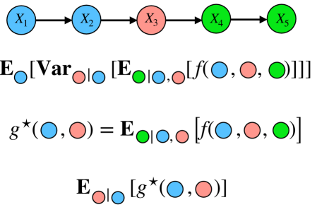
We propose a new family of trajectory-wise CVs, called TrajCV, that improves upon existing state or state-action CV techniques by tackling additionally $\mathbf{Var}_{|S_{t},A_{t}}$, the variance due to randomness in trajectory after step $t$ (cf. Section 3). While this idea sounds intuitively pleasing, a technical challenge immediately arises. Recall in designing CVs, we need to know the expectation of the proposed CV function over the randomness that we wish to reduce (see (3)). In this case, suppose we propose a CV $g(S_{t},A_{t},\dots,A_{h-1},S_{h})$, we would need to know its conditional expectation $\mathbf{E}_{|S_{t},A_{t}}[g(S_{t},A_{t},\dots,S_{h},A_{h})]$. This need makes reducing $\mathbf{Var}_{|S_{t},A_{t}}$ fundamentally different from reducing $\mathbf{Var}_{A_{t}|S_{t}}$, the latter of which has been the main focus in the literature: Because the dynamics $d$ is unknown, we do not have access to the distribution of trajectories after step $t$ and therefore cannot compute $\mathbf{E}_{|S_{t},A_{t}}$; by contrast, reducing $\mathbf{Var}_{A_{t}|S_{t}}$ only requires knowing the policy $\pi$.

At first glance this seems like an impossible quest. But we will show that by a clever divide-and-conquer trick, an unbiased CV can actually be devised to reduce the variance $\mathbf{Var}_{|S_{t},A_{t}}$. The main idea is to 1) decompose $\mathbf{Var}_{|S_{t},A_{t}}$ through repeatedly invoking the law of total variance and then 2) attack the terms that are amenable to reduction using CVs. As expected, the future variance cannot be completely reduced, because of the unknown dynamics. But we should be able to reduce the randomness due to known distributions, namely, the future uses of policy $\pi$.

(a) CV on a toy problem

(b) effects of state-action CV and TrajCV

Figure 1: (a) An illustration of the Divide-and-Conquer strategy on the toy problem in Section 4.1 using color encoding. First row: ordering and coloring of the random variables. Second row: the variance to reduce, i.e. the variance due to the randomness of variables in red circle. Third row: the corresponding optimal CV. Last row: the expectation required to compute the difference estimator for the optimal CV. (b) An illustration of the effect of state-action CV (6) and TrajCV (4.2) on each policy gradient component $G_{t}$. Each row corresponds to each $G_{t}$, and each column corresponds to one term in the total variance of $G_{t}$. For example, the $A_{2}$ column is associated with the term $\mathbf{E}_{S_{1,2},A_{1}}\mathbf{Var}_{A_{2}|S_{2}}\mathbf{E}_{|S_{2},A_{2}}\left[G_{t}\right]$. The state-action CVs influence the terms in red, whereas TrajCV additionally affect the terms in blue.

4.1 A Divide-and-Conquer Strategy

Before giving the details, let us first elucidate our idea using a toy problem. Consider estimating $\mathbf{E}\left[f(X_{1,5})\right]$, the expectation of a function $f$ of $5$ random variables, where the subscript _i,j denotes the collection of random variables, i.e. $X_{1,5}=\{X_{1},\dots,X_{5}\}$. We can apply the law of total variance repeatedly, in the order indicated by the subscript, and decompose the variance into

$$\textstyle\mathbf{Var}\left[f(X_{1,5})\right]=\sum_{k=1}^{5}\mathbf{E}_{X_{1,k-1}}\mathbf{Var}_{X_{k}|X_{1,k-1}}\mathbf{E}_{X_{k+1,n}|X_{1,k}}[f(X_{1,5})]$$ (10)

For example, suppose we wish to reduce $\mathbf{Var}_{X_{3}|X_{1,2}}$ we simply need to consider a CV in the form $g\left(X_{1,3}\right)$, which does not depends on random variables with larger indices. With the difference estimator $f(X_{1,5})-g\left(X_{1,3}\right)+\mathbf{E}_{X_{3}|X_{1,2}}[g\left(X_{1,3}\right)]$, the variance $\mathbf{Var}_{X_{3}|X_{1,2}}$ changes into

$$\mathbf{E}_{X_{1,2}}\mathbf{Var}_{X_{3}|X_{1,2}}[\mathbf{E}_{X_{4,5}|X_{1,3}}[f(X_{1,5})]-g(X_{1,3})]$$

Apparently when $g$ is optimally chosen as $g^{\star}(X_{1,3}):=\mathbf{E}_{X_{4,5}|X_{1,3}}[f(X_{1,5})]$, this term vanishes.

Fact 1 A key property of designing CVs by the recursive decomposition above is that the inclusion of the extra term, e.g. $g\left(X_{1,3}\right)-\mathbf{E}_{X_{3}|X_{1,2}}\left[g(X_{1,3})\right]$, in the difference estimator only affects a single component $\mathbf{Var}_{X_{3}|X_{1,2}}$ in the total variance, without influencing the other terms. This separation property hence allows for a divide-and-conquer strategy: we can design CVs for each term separately and then combine them; the reduction on each term will add up and reduce the total variance.

Fact 2 There is still one missing piece before we can adopt the above idea to design CVs for estimating policy gradients: the ordering of random variables. In the example above, we need to know $\mathbf{E}_{X_{3}|X_{1,2}}\left[g(X_{1,3})\right]$ to compute the difference estimator. Namely, it implicitly assumes the knowledge about $p(X_{3}|X_{1,2})$, which may or may not be accessible. Suppose $p(X_{3}|X_{1,2})$ is not available but $p(X_{3}|X_{4,5})$ is. We can consider instead using the law of total variance in a different order, e.g. $X_{4}\rightarrow X_{5}\rightarrow X_{3}\rightarrow X_{1}\rightarrow X_{2}$, and utilize the information $p(X_{3}|X_{4,5})$ to construct a difference estimator to reduce $\mathbf{Var}_{X_{3}|X_{4,5}}$. Therefore, the design of CVs hinges also on the information available. Recall that we only know about the policy but not the dynamics in RL.

4.2 Design of TrajCV

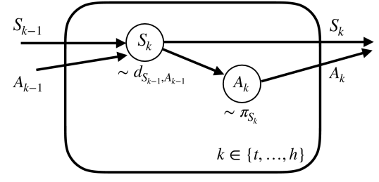
After fleshing out the idea in the example above, we are now ready to present TrajCVs for policy gradient. Again let us focus on a policy gradient component $G_{t}$ for transparency. Recall that $G_{t}$ is a function of the random variables $S_{t,h}$ and $A_{t,h}$. Given the information we know about the random variables (i.e. the policy) and the Markovian structure depicted in the Bayes network in Figure 2(a), a natural ordering of them for applying law of total variance is

$$S_{t}\rightarrow A_{t}\rightarrow S_{t+1}\rightarrow A_{t+1}\rightarrow\dots\rightarrow S_{h}\rightarrow A_{h}.$$ (11)

Thanks to the Markovian structure, $\mathbf{Var}_{A_{k}|S_{1,k},A_{1,k-1}}$ can be simplified into $\mathbf{Var}_{A_{k}|S_{k}}$. Thus, for reducing $\mathbf{Var}_{A_{k}|S_{k}}$, we may consider a CV, $\widehat{g}^{(t)}(S_{k},A_{k})$, where the superscript ^(t) is a reminder of estimating $\mathbf{E}\left[G_{t}\right]$. With the insights from Section 4.1, we see the optimal choice of $\widehat{g}^{(t)}$ is

$$\widehat{g}^{(t)\star}(S_{k},A_{k}) =\mathbf{E}_{S_{k+1,h},A_{k+1,h}|S_{k},A_{k}}\left[N_{t}C_{t:h}\right]=N_{t}\left(C_{t:k-1}+q^{\pi}(S_{k},A_{k})\right),$$

suggesting practically we can use $\widehat{g}^{(t)}(S_{k},A_{k}):=N_{t}(C_{t:k-1}+\widehat{Q}_{k})$, where $\widehat{Q}_{k}:=\widehat{q}(S_{k},A_{k})$ and $\widehat{q}\approx q^{\pi}$ as was in (6). In other words, we showed that finding the optimal CV for reducing $\mathbf{Var}_{A_{k}|S_{k}}$ can be reduced to learning the Q-function; this enables us to take advantage of existing policy evaluation algorithms. Now we combine $\{\widehat{g}^{(t)}(S_{k},A_{k})\}_{k=t}^{h}$ to build the CV for $G_{t}$. Because from Section 4.1 these terms do not interfere with each other, we can simply add them together, yielding TrajCV: $\sum_{k=t}^{h}\widehat{g}^{(t)}(S_{k},A_{k})$. Equivalently, we have derived a difference estimator:

$${\widetilde{G}^{\mathrm{Traj},\widehat{q}}}_{t} :=\textstyle G_{t}-\sum_{t=1}^{h}\left(\widehat{g}^{(t)}(S_{k},A_{k})-\mathbf{E}_{A_{k}|S_{k}}[\widehat{g}^{(t)}(S_{k},A_{k})]\right)$$

$$=\textstyle G_{t}-\sum_{k=1}^{h}\left(N_{t}\widehat{Q}_{k}-\mathbf{E}_{A_{k}|S_{k}}[N_{t}\widehat{Q}_{k}]\right)$$ (12)

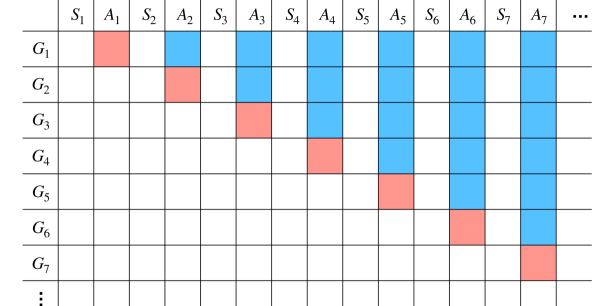
Comparing TrajCV in (4.2) and state-action CV in (5), we see that the state-action CV only contains the first term in the summation of TrajCV. The remaining terms, i.e. $N_{t}(\widehat{Q}_{k}-\mathbf{E}_{A_{k}|S_{k}}[\widehat{Q}_{k}])$, for $t<k\leq h$, can be viewed as multiplying $N_{t}$ with estimates of future advantage functions. Appealing to law of total variance, $\mathbf{Var}[{\widetilde{G}^{\mathrm{Traj},\widehat{q}}}_{t}]$ can be decomposed into

$$\mathbf{Var}_{S_{t}}\mathbf{E}_{|S_{t}}\left[N_{t}C_{t:h}\right]+\mathbf{E}_{S_{t}}\mathbf{Var}_{A_{t}|S_{t}}[N_{t}(\mathbf{E}_{|S_{t},A_{t}}\left[C_{t:h}\right]-\widehat{Q}_{t})]+$$ (13)

$$\sum_{k=t}^{h}\mathbf{E}_{S_{k},A_{k}}\mathbf{Var}_{S_{k+1}|S_{k},A_{k}}\left[N_{t}\mathbf{E}_{|S_{k+1}}[C_{k:h}]\right]+\sum_{k=t}^{h}\mathbf{E}_{S_{k+1}}\mathbf{Var}_{A_{k+1}|S_{k+1}}[N_{t}(\mathbf{E}_{|S_{k+1},A_{k+1}}[C_{k:h}]-\widehat{Q}_{k+1})]$$

where we further decompose the effect of $\mathbf{Var}_{|S_{t},A_{t}}$ in the second line into the randomness in dynamics and actions, respectively. Therefore, suppose the underlying dynamics is deterministic (i.e. $\mathbf{Var}_{S_{k+1}|S_{k},A_{k}}$ vanishes), and $\widehat{q}=q^{\pi}$, then using TrajCV (4.2) would completely remove $\mathbf{Var}_{A_{t}|S_{t}}$ and $\mathbf{Var}_{|S_{t},A_{t}}$, the latter of which previous CVs (5) and (6) cannot affect. In Fig. 1(b), we visualize the effect of TrajCV and state-action CV on each policy gradient component $G_{t}$, for $1\leq t\leq h$: state-action CVs only influence the diagonal terms, while TrajCVs are able to affect the full upper triangle terms. Note that in implementation of TrajCV for $G_{1:h}$, we only need to compute quantities $\widehat{Q}_{t}$, $\mathbf{E}_{A_{t}|S_{t}}[\widehat{Q}_{t}]$ and $\nabla\mathbf{E}_{A_{t}|S_{t}}[\widehat{Q}_{t}]$ along a trajectory (done in $O(h)$ time) and they can be used to compute $\{{\widetilde{G}^{\mathrm{Traj},\widehat{q}}}_{t}\}_{t=1}^{h}$ (4.2). In addition, we remark that when $\widehat{q}(s,a)=\widehat{v}(s)$, TrajCV reduces to the state-dependent CVs.

(a) before policy reparameterization

(b) after policy reparameterization

Figure 2: Bayes networks for the random variables in $G_{t}$ (2), before and after reparameterization. After policy is reparameterized, action $A_{k}$ is decided by state $S_{k}$ and action randomness $R_{k}$.

4.3 The Natural Ordering in (11) is Optimal

Recall in Section 4.1 we mentioned that the admissible ordering of random variables used in invoking the law of total variance depends on the information available. Here we show that the chosen ordering (11) is indeed, the best ordering to adopt, as we only know the policy, not the dynamics.

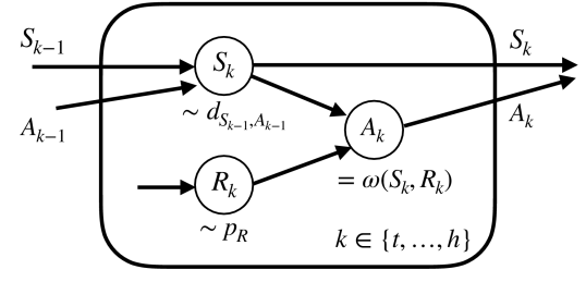
We compare (11) against potential orderings constructed by reparameterizing the policy such that its randomness in action becomes independent of the input state. We suppose the policy $\pi\in\Pi$ can be reparameterized by a function $\omega:{\mathcal{S}}\times{\mathcal{R}}\to\mathcal{A}$ and a distribution $p_{R}$, so that for all $s\in{\mathcal{S}}$, $\omega(s,R)$ and $\pi_{s}$ are equal. This is not a restricted assumption. For example, a Gaussian stochastic policy with mean $\mu_{\theta}(s)$ and covariance $\Sigma(s)$, widely used in continuous domains [1, 5, 40], can be framed as $\omega(s,R)=\mu(s)+\Sigma^{1/2}(s)R$, where $R$ is multivariate standard normal. Even when $\mathcal{A}$ is discrete, a soft-max layer can be applied after $\omega$ to obtain a Gibbs (or Boltzmann) distribution [41, 2].

Reparameterization gives rise to the chance of designing a larger family of TrajCVs. By extracting the randomness in action selection into the random variable $R_{t,h}$, the policy gradient component $G_{t}$ becomes a function of $R_{t,h}$ and $S_{t,h}$, as depicted in the Bayes network in Figure 2(b). When applying the law of total variance, the ordering the random variables now can have many possibilities. For instance, in the extreme case, the randomness of actions can be ordered before states (except $S_{t}$) as

$$S_{t}\rightarrow R_{t}\rightarrow\dots\rightarrow R_{h}\rightarrow S_{t+1}\rightarrow\dots\rightarrow S_{h},$$ (14)

leading to a CV that’s a function of $R_{t,h}$ bearing the optimal choice $\mathbf{E}_{S_{t+1,h}|R_{t,h},S_{t}}\left[N_{t}C_{t:h}\right]$. Note that $\mathbf{E}_{S_{t+1,h}|R_{t,h},S_{t}}\left[N_{t}C_{t:h}\right]$ is a function that inputs the observable action randomness $R_{t,h}$, not the randomness of the unknown dynamics. Therefore, it can be approximated, e.g., if we have a biased simulator of the dynamics. One might ask, given all possible orderings of random variables, which ordering we should pick to design the CV. Interestingly, to this question, the most natural one and the optimal one coincide. The proof is deferred to Appendix A.

Theorem 4.1.

Suppose that policy specified by $\omega$ and $p_{R}$ is known, but the dynamics $d$ is unknown. Assume the optimal CV of a given ordering of random variables $S_{t,h}$ and $R_{t,h}$ can be obtained. The the optimal ordering that minimizes the residue variance is the natural ordering (11) .

Theorem 4.1 tells us that if the optimal CVs are attainable (i.e. we can estimate the Q-function exactly), then the natural ordering is optimal. However, in practice, the CVs are almost always suboptimal due to error in estimation. If the dynamics is relatively accurate and the computing resources for simulation are abundant, then although the residue is higher, the ordering (14) could actually be superior. Therefore, the ordering of random variables based on the relative accuracy of different estimates is an interesting practical question to pursue in future work. In the experiment section of this work, we will focus on the natural ordering (11).

5 Experimental Results and Discussion

Although the focus of this paper is the theoretical insights, we illustrate our results with experiments in learning neural network policies to solve the CartPole balancing task in OpenAI Gym [42] with DART physics engine [43]. In CartPole, the reward function is the indicator function that equals to one when the pole is close to being upright and zero otherwise. This is a delayed reward problem in that the effective reward signal is revealed only when the task terminates prematurely before reaching the horizon, i.e. when the pole deviates from being upright. The start state is perturbed from being vertical and still by an offset uniformly sampled from $[-0.01,0.01]^{d_{\mathcal{S}}}$, and the dynamics is deterministic. The action space is continuous and Gaussian policies are considered in the experiments. The policy is optimized by natural gradient descent [3] with a KL-divergence safe guard on the policy change to be robust to outliers in data collection. Below we report in rewards, negative of costs, which is the natural performance measure provided in OpenAI Gym.

(a) $\sigma=0.1$

(b) $\sigma=0.3$

(c) $\sigma=1.0$

(d) $\sigma=3.0$

Figure 3: The size of components of $\mathop{\bf Tr}\left(\mathbf{Var}[G_{t}]\right)$ during training, for $t=100$, evaluated at policies generated under the “upper bound” setting that emulates noiseless estimates for the CartPole problem with horizon $h=1000$. Different initial values for $\sigma$ of the Gaussian policy (defined in Theorem 3.1) are used. The $x$ axis denotes the iteration, and the $y$ axis is in $\log$ scale. The two vertical dashed lines mark the boundaries of iterations where the expected accumulated rewards is between $50$ and $900$.

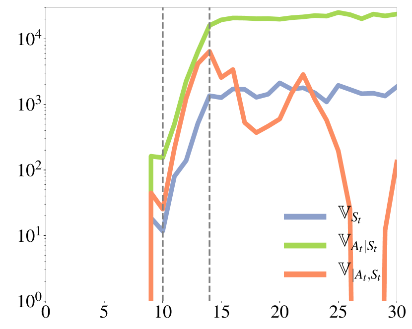
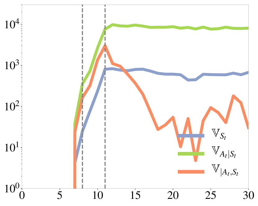
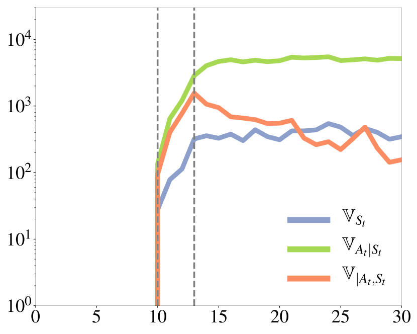
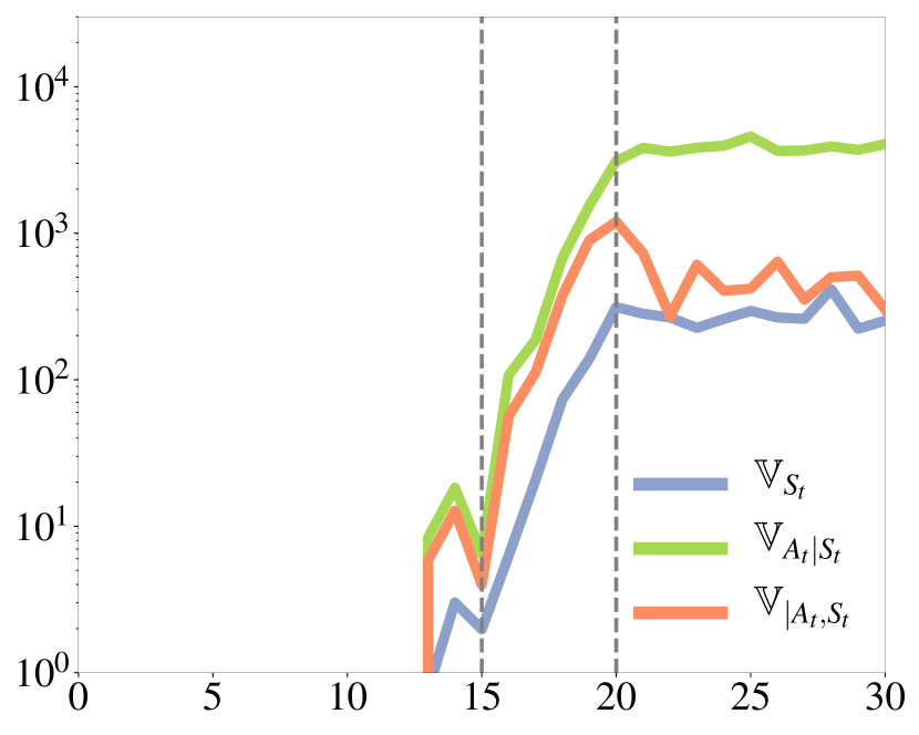
In Fig. 3, we corroborate the theoretical findings in Theorem 3.1 by empirically evaluating the components of $\mathop{\bf Tr}\left(\mathbf{Var}[G_{t}]\right)$ during learning, for $t=100$. The learning process on CartPole can be partitioned into three stages: 1) initial exploration, when the policy performs very poorly and improves slowly, 2) rapid improvement, when the policy performance increases steeply, 3) near convergence, when the policy reaches and stays at the peak performance. The dashed vertical lines in Fig. 3 delimit these three stages. In the rapid improvement stage, due to the variance in the accumulated rewards, i.e. length of the trajectories, $\mathbb{V}_{|A_{t},S_{t}}$ is large, close to $\mathbb{V}_{A_{t}|S_{t}}$ and about 10 times of $\mathbb{V}_{S_{t}}$ as predicted by Theorem 3.1. Furthermore, as $\sigma$ increases, the gap between the peak values of $\mathbb{V}_{S_{t}}$ and $\mathbb{V}_{A_{t}|S_{t}}$ narrows.

(a) $h=1000$ (MC)

(b) $h=2000$ (MC)

(c) $h=4000$ (MC)

Figure 4: The results of naive Monte Carlo estimate of policy gradient, and it augmented with state CV, state-action CV, and TrajCV on CartPole problems with horizon $h=1000,2000,4000$. “MC” in the legend indicates that the expectation over actions for state-action CV and TrajCV is approximated using Monte Carlo (1000 samples). Upper bound emulates the results of noiseless estimates. The $x$ and $y$ axes are iteration number and accumulated rewards (the higher the better), respectively. The median of 8 random seeds is plotted, and the shaded area accounts for 25% percentile.

(a) $h=4000$ (diff)

(b) $h=4000$ (next)

Figure 5: The exact same settings as Fig. 4 except that the state-action CV and TrajCV are given by $\widehat{q}^{(\text{diff})}$ and $\widehat{q}^{(\text{diff-GN})}$ (Fig. 5(a)), and $\widehat{q}^{(\text{next})}$ and $\widehat{q}^{(\text{next-GN})}$ (Fig. 5(b)).

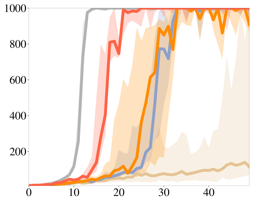
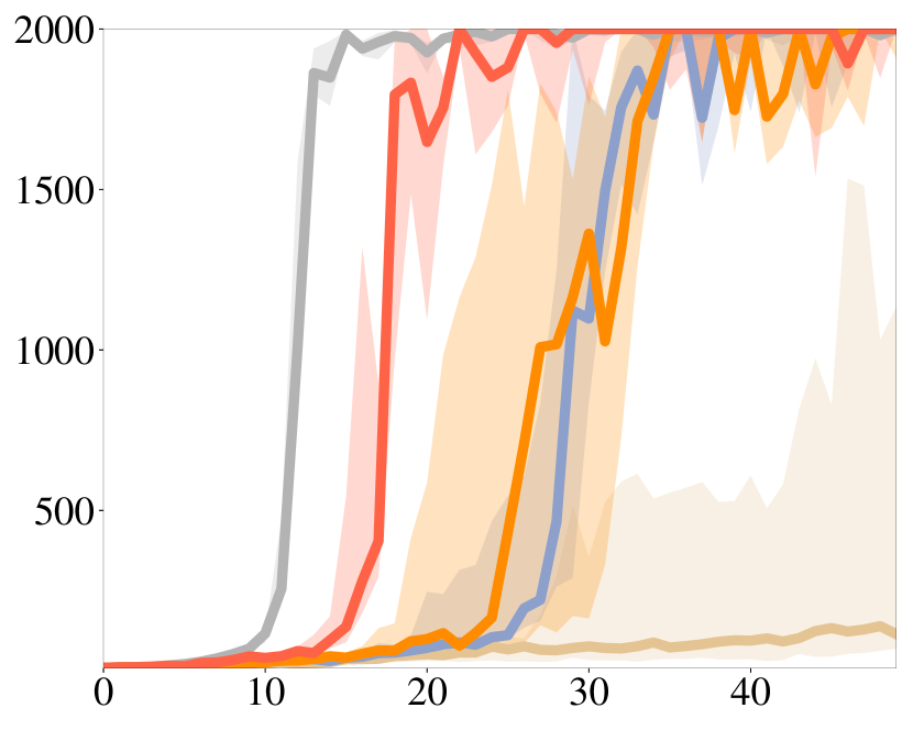
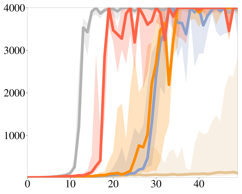
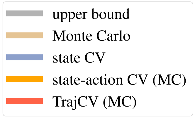
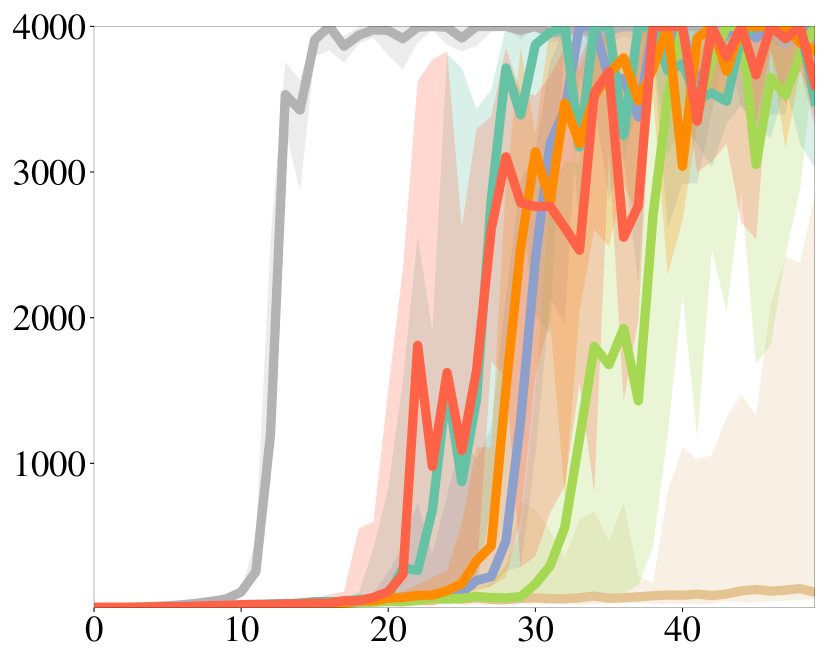
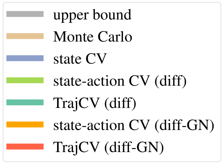
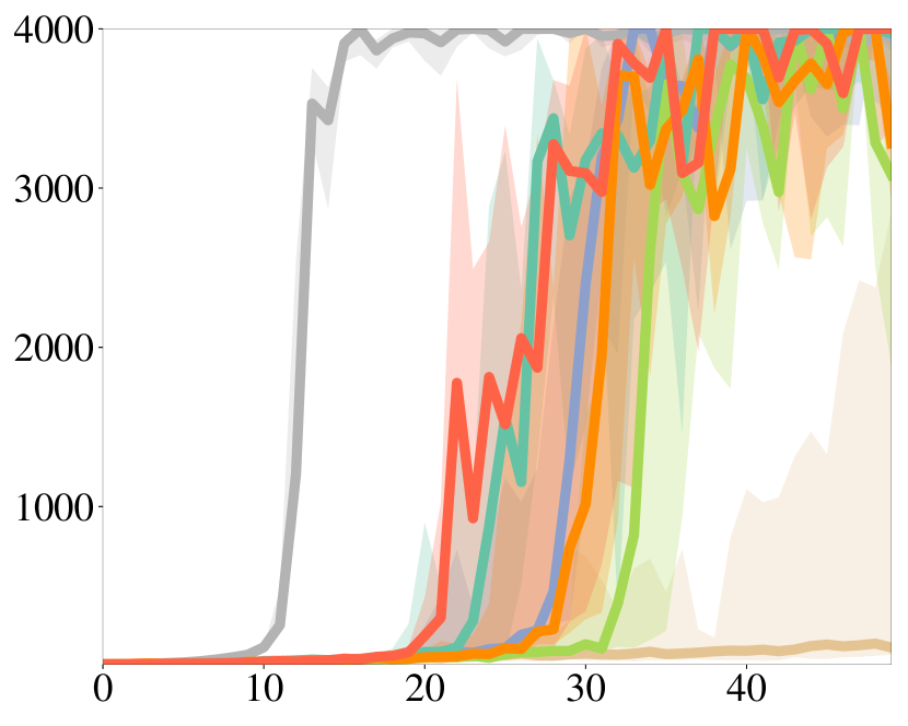
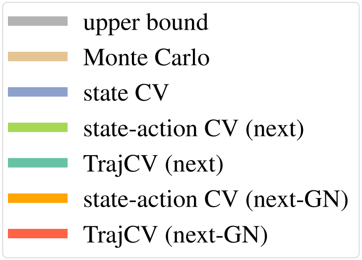
We compare naive Monte Carlo estimate (2), state dependent CV (5), state-action CV (6), and TrajCV (4.2), in Fig. 4 and Fig. 5. To facilitate a fair comparison, we realize all algorithms with the same implementation based on an on-policy value function approximator $\widehat{v}$, so that the effects of value estimates’ quality can be normalized. More concretely, $\widehat{v}$ is learned by sampling abundant data from a biased dynamics model (which is obtained by perturbing the underlying physical parameters).

To construct the Q-function approximator $\widehat{q}$ required by the state-action CV and TrajCV, we further train a deterministic function $\widehat{d}$ that maps the current state and action to next state using the same data from the environment that are used for computing the policy gradient estimates. Combining the value function approximator $\widehat{v}$ and the dynamics approximator $\widehat{d}$ yields a natural Q-function approximator $\widehat{q}^{\text{(dyn)}}(s,a)=c(s,a)+\widehat{v}(\widehat{d}(s,a))$. Based on this basic $\widehat{q}^{\text{(dyn)}}$, we explored several options of Q-function approximator for defining the state-action CV and TrajCV:

1. Monte Carlo (MC) : $\widehat{q}^{\text{(dyn)}}(s,a)$. We use many samples of actions (1000 in the experiments) to approximate $\mathbf{E}_{A_{t}|S_{t}}\left[\widehat{q}^{\text{(dyn)}}(S_{t},A_{t})\right]$. To reduce variance, we use the same action randomness for different steps, i.e. using the same 1000 i.i.d. samples from $p_{R}$ (defined in Section 4.3) in the evaluation for $\mathbf{E}_{A_{t}|S_{t}}$ with different $t$.

2. We also consider various Q-function approximators that are quadratic in action, so that $\mathbf{E}_{A_{t}|S_{t}}$ can be evaluated in closed-form. They are derived by different linearizations of the Q-function approximator $\widehat{q}$ as shown below.

   1. $\widehat{q}^{(\text{next})}(s,a)=c(s,a)+\widehat{v}(\widehat{s}^{\prime})+(a-m)^{\top}\nabla_{m}\widehat{d}(s,m)\nabla\widehat{v}(\widehat{s}^{\prime}),$

   2. $\widehat{q}^{(\text{next-GN})}(s,a)=\widehat{q}^{(\text{next})}(s,a)+\frac{1}{2}(a-m)^{\top}\nabla_{m}\widehat{d}(s,m)\nabla^{2}\widehat{v}(\widehat{s}^{\prime})\nabla_{m}\widehat{d}(s,m)^{\top}(a-m),$

   3. $\widehat{q}^{(\text{diff})}(s,a)=\widehat{v}(s)+(a-m)^{\top}\nabla_{m}(c(s,m)+\widehat{v}(\widehat{s}^{\prime}))+\frac{1}{2}(a-m)^{\top}\nabla_{m}^{2}c(s,m)(a-m),$

   4. $\widehat{q}^{(\text{diff-GN})}(s,a)=\widehat{q}^{(\text{diff})}(s,a)+\frac{1}{2}(a-m)^{\top}\nabla_{m}\widehat{d}(s,m)\nabla^{2}\widehat{v}(\widehat{s}^{\prime})\nabla_{m}\widehat{d}(s,m)^{\top}(a-m),$

   where $m=\mu_{\theta}(s)$ is the mean of the Gaussian policy, $\widehat{s}^{\prime}=\widehat{d}(s,m)$, and “GN” stands for Gauss-Newton. We assume $c(s,a)$ is quadratic in $a$ for $\widehat{q}^{(\text{next})}$ and $\widehat{q}^{(\text{next-GN})}$.

The performance of different CVs using MC for approximating $\mathbf{E}_{A_{t}|S_{t}}$ is reported in Fig. 4, where 5 rollouts are sampled for each iteration. We also emulate noise-free gradients, denoted as upper bound, which is constructed by running the state dependent CV but with $100,000$ samples per iteration. Overall when more information is used to design the CVs (from state only, state-action, and then trajectory-wise) the convergence speed improves. In particular, as the problem horizon becomes longer, the gap becomes larger: the reward feedback becomes sparser, so the variance due to long-term trajectory starts to dominate, as shown in Fig. 4(c). In Fig. 5, we observe that when $\mathbf{E}_{A_{t}|S_{t}}$ is approximated analytically using various techniques ($\widehat{q}^{(\text{next})}$ and $\widehat{q}^{(\text{next-GN})}$ are the CVs suggested in [20] and [24], respectively), learning is accelerated when more information is leveraged in CV synthesis.

These preliminary experimental results support the theoretical insights provided in Section 3 and Section 4, suggesting the importance of considering long-term effects in designing CVs, especially for problems with a long horizon. The fix turns out to be quite simple: just padding additional terms (cf. (4.2)) onto the existing CVs, which can be done using Q-function approximators available in existing CVs without new information. Interestingly we prove this simple idea is optimal. Important future work includes considering the different bias and variance trade-off discussed in Section 4.3, and learning the linear combination weights of the CVs for policy gradient components $\{G_{t}\}_{t=1}^{h}$.

Acknowledgments

This work was partially supported by NSF CAREER award 1750483.

Appendix

Appendix A Missing Proofs

A.1 Proof for Theorem 4.1

To understand how the ordering matters, we consider a toy example of estimating $\mathbf{E}_{X,Y}[f(X,Y)]$ of some function $f$ of two random variables $X$ and $Y$. We prove a basic lemma.

Lemma A.1.

If $X$ and $Y$ are independent, then

$$\mathbf{Var}_{X}\mathbf{E}_{Y}\left[f(X,Y)\right]\leq\mathbf{E}_{Y}\mathbf{Var}_{X}\left[f(X,Y)\right]$$ (15)

Proof.

This can be proved by Jensen’s inequality.

$$\mathbf{Var}_{X}\mathbf{E}_{Y}\left[f\right]=\mathbf{E}_{X}\left(\mathbf{E}_{Y}\left[f-\mathbf{E}_{X}\left[f\right]\right]\right)^{2}\leq\mathbf{E}_{X}\mathbf{E}_{Y}\left[\left(f-\mathbf{E}_{X,Y}\left[f\right]\right)^{2}\right]=\mathbf{E}_{Y}\mathbf{Var}_{X}\left[f(X,Y)\right]$$

∎

Suppose we want to reduce the variance of estimating $\mathbf{E}_{X,Y}[f(X,Y)]$ with some CV $g(X,Y)$ but only knowing the distribution $P(X)$, not $P(Y)$. Lemma A.1 tells us that in decomposing the total variance of $f(X,Y)$ to design this CV (cf. Section 2.3) we should take the decomposition

$$\mathbf{Var}_{Y}\mathbf{E}_{X}\left[f(X,Y)\right]+\mathbf{E}_{Y}\mathbf{Var}_{X}\left[f(X,Y)\right]$$ (16)

instead of the decomposition

$$\mathbf{Var}_{X}\mathbf{E}_{Y}\left[f(X,Y)\right]+\mathbf{E}_{X}\mathbf{Var}_{Y}\left[f(X,Y)\right]$$ (17)

In other words, we should take the ordering $Y\to X$, instead of $X\to Y$, when we invoke the law of total variance. The reason is that after choosing the optimal CV for each case to reduce the variance due to $X$ (the information that we have access to), we are left with $\mathbf{Var}_{Y}\mathbf{E}_{X}\left[f(X,Y)\right]$ and $\mathbf{E}_{X}\mathbf{Var}_{Y}\left[f(X,Y)\right]$, respectively, for $Y\to X$ and $X\to Y$. By Lemma A.1, we see the $Y\to X$ has a smaller residue in variance. In other words, when we only have partial information about the distribution, we should arrange the random variables whose distribution we know to the latter stage of the ordering, so that the CV we design can leverage the sampled observations to compensate for the lack of prior.

We use this idea to prove the natural ordering Eq. 11 in optimal. In analogy of $X$ and $Y$, we have the action randomness whose distribution is known (i.e. the policy) and the dynamics randomness, whose distribution is unknown.

The potential orderings we consider come from first reparameterizing the policy and then ordering the independent random variables $R_{t}$ (cf. Section 4.3). We note that the CV is determined by the ordering, not due to reparameterization. For the natural ordering,

$$S_{t}\rightarrow A_{t}\rightarrow S_{t+1}\rightarrow A_{t+1}\rightarrow\dots\rightarrow S_{h}\rightarrow A_{h},$$ (11)

it gives the same control variate of the ordering below based on reparameterization

$$S_{t}\rightarrow R_{t}\rightarrow S_{t+1}\rightarrow R_{t+1}\rightarrow\dots\rightarrow S_{h}\rightarrow R_{h}.$$ (18)

Suppose that given an ordering, we can compute its optimal CV. We define the variance left after applying that optimal CV associated with the ordering, the residue of that ordering. We will show that the residue is minimized at the natural ordering.

The proof consists of two steps.

1. We show that when dynamics is the MDP is unknown, an ordering is feasible, if and only if, $R_{k}$ appears before $S_{k+1,h}$ for all $t\leq k<h$. That is, a feasible ordering must be causal at least in actions: the action randomness that causes a state must be arranged before that state in the ordering. We prove this by contradiction. Assume otherwise $S_{u}$ is the first state before $R_{k}$ satisfying $u>k$. We see that $R_{k}$ and $S_{u}$ are dependent, if none of the variables in $S_{k+1,u}$ is given. This observation can been inferred from the Bayes network that connect these random variables (Fig. 2(b)), i.e. the path from $R_{t}$ to $S_{u}$ is not blocked unless any of $S_{k+1,u}$ is observed [44]. Therefore, if we have an ordering that is violates the causality property defined above, the expectation over $R_{k}$ required to define the difference estimator becomes intractable to compute, because the dynamics is unknown. This creates a contradiction.

2. We show that any feasible ordering can be transformed into the natural ordering in (11) using operations that do not increase the residue. We consider the following operations

   1. Suppose, in an ordering, there is $S_{v}\rightarrow S_{u},v>u$, then we can exchange them without affecting residue.

   2. Suppose, in a feasible ordering, there is $S_{v}\rightarrow R_{k}\rightarrow S_{u}$ with $v>u$ and $k\neq u,v$. Because this is a feasible ordering, we have $k+1\leq u<v$. This means that we can also move $R_{k}$ after $S_{u}$. This change would not increase residue, because of the discussion after Lemma A.1. Then we change exchange the order of $S_{v}$ and $S_{u}$ too using the first operation.

   By using these two operations repeatedly, we can make all the states ordered by their subscripts, without increasing the residue. Finally, we can move $R_{k}$ to just right after $S_{k}$ without increasing residue using Lemma A.1 again. Thus, we arrive at the natural ordering in (18), which is the same as (11). This concludes the proof.

A.2 Proof of Theorem 3.1

Suppose the dimension of $\mathcal{A}$ is $d_{\mathcal{A}}$ which is finite. To bound these terms, we derive some intermediate bounds. First, by the Gaussian assumption,

$$\pi_{S_{t}}(A_{t})=(2\pi\sigma)^{-\frac{d_{\mathcal{A}}}{2}}\exp\left(\frac{-1}{2\sigma}\left\|A_{t}-\mu_{\theta}(S_{t})\right\|^{2}\right)$$

we see that

$$N_{t}:=\nabla\ln\pi(A_{t}|S_{t})=\begin{bmatrix}\nabla_{\theta}\ln\pi(A_{t}|S_{t})\\ \nabla_{\sigma}\ln\pi(A_{t}|S_{t})\end{bmatrix}=\begin{bmatrix}\frac{-1}{\sigma}\nabla\mu_{\theta}(S_{t})(A_{t}-\mu_{\theta}(S_{t}))\\ \frac{1}{2\sigma^{2}}\left\|A_{t}-\mu_{\theta}(S_{t})\right\|^{2}-\frac{d_{\mathcal{A}}}{2\sigma}\end{bmatrix}$$

Therefore, for $\sigma$ small enough, $\left\|N_{t}\right\|=O(\frac{{\mathrm{poly}}(A_{t})}{\sigma^{2}})$.

Second, by the assumption on boundedness of $C$, we have $C_{t:h}=O(h)$ and $Q_{t}\coloneqq q^{\pi}(S_{t},A_{t})=O(h)$. We use these equalities to bound $\mathbf{E}_{|S_{t}}\left[N_{t}C_{t:h}\right]$. We observe that the identity that

$$\mathbf{E}_{|S_{t}}\left[N_{t}C_{t:h}\right]=\nabla\mathbf{E}_{A_{t}|S_{t}}[q^{\pi}(S_{t},A_{t})]$$

Under the assumption that $q^{\pi}$ is analytic, $q^{\pi}$ can be written in terms of an infinite sum of polynomials, i.e. $q^{\pi}(S_{t},A_{t})={\mathrm{poly}}_{S_{t}}(A_{t})$, where the subscript denotes the coefficients in the polynomial depends on $S_{t}$.

Now we are ready to bound $\mathbb{V}_{S_{t}}$, $\mathbb{V}_{A_{t}|S_{t}}$, and $\mathbb{V}_{|S_{t},A_{t}}$. We recall that the expectation of polynomials over a Gaussian distribution depends only polynomially on the Gaussian’s variance, with an order no less than $1$. Therefore, for $\sigma$ small enough, we have $\left\|\nabla\mathbf{E}_{A_{t}|S_{t}}[q(S_{t},A_{t})]\right\|=O(h)$ independent of $\sigma$, which implies that

$$\mathbb{V}_{S_{t}} =\mathop{\bf Tr}\left(\mathbf{Var}_{S_{t}}\left[\mathbf{E}_{|S_{t}}\left[N_{t}C_{t:h}\right]\right]\right)=o(h^{2})$$

We can apply the same observation on the Gaussian expectation of polynomials and derive, for $\sigma$ small enough,

$$\mathbb{V}_{A_{t}|S_{t}} =\mathop{\bf Tr}\left(\mathbf{E}_{S_{t}}\left[\mathbf{Var}_{A_{t}|S_{t}}\left[N_{t}\left(\mathbf{E}_{|S_{t},A_{t}}\left[C_{t:h}\right]\right)\right]\right]\right)$$

$$=\mathop{\bf Tr}\left(\mathbf{E}_{S_{t}}\left[\mathbf{Var}_{A_{t}|S_{t}}\left[N_{t}q^{\pi}(S_{t},A_{t})\right]\right]\right)=O\left(\frac{h^{2}}{\sigma^{4}}\right)$$

Similarly we can show

$$\mathbb{V}_{|S_{t},A_{t}} =\mathop{\bf Tr}\left(\mathbf{E}_{S_{t},A_{t}}[\mathbf{Var}_{|S_{t},A_{t}}\left[N_{t}C_{t:h}\right]]\right)=O\left(\frac{h^{2}}{\sigma^{4}}\right)$$

This concludes the proof.

A.3 Bound for Variance of Policy Gradient

The variance of the policy gradient $\mathbf{Var}[G]$ can be bounded by the variance of policy gradient components $\{\mathbf{Var}[G_{t}]\}_{t=1}^{n}$. Appealing to the formula for the variance of the sum of two random variables

$$\mathbf{Var}[X+Y]=\mathbf{Var}[X]+\mathbf{Var}[Y]+2\mathbf{Cov}[X,Y],$$

linearity of covariance

$$\mathbf{Cov}[X,Y+Z]=\mathbf{Cov}[X,Y]+\mathbf{Cov}[X,Z]$$

and Cauchy -Schwartz inequality

$$\mathbf{Cov}[X,Y]\leq\mathbf{Var}[X]+\mathbf{Var}[Y],$$

we can derive the following:

$$\quad\;\mathbf{Var}[G] =\mathbf{Var}\left[G_{1:h}\right]$$

$$=\mathbf{Var}\left[G_{1}\right]+\mathbf{Var}\left[G_{2:h}\right]+\mathbf{Cov}[G_{1},G_{2:h}]$$

$$=\mathbf{Var}[G_{1}]+\sum_{t=2}^{h}\mathbf{Cov}[G_{1},G_{t}]+\mathbf{Var}\left[G_{2:h}\right]$$

$$=\sum_{t=1}^{h}\mathbf{Var}[G_{t}]+\sum_{u=1}^{h}\sum_{v=u+1}^{h}\mathbf{Cov}[G_{u},G_{v}]$$

$$\leq\sum_{t=1}^{h}\mathbf{Var}[G_{t}]+\sum_{u=1}^{h}\sum_{v=u+1}^{h}\left(\mathbf{Var}[G_{u}]+\mathbf{Var}[G_{v}]\right)$$

$$=h\sum_{t=1}^{h}\mathbf{Var}[G_{t}]$$

References

- Williams [1992] R. J. Williams. Simple statistical gradient-following algorithms for connectionist reinforcement learning. Machine learning, 8(3-4):229–256, 1992.
- Sutton et al. [2000] R. S. Sutton, D. A. McAllester, S. P. Singh, and Y. Mansour. Policy gradient methods for reinforcement learning with function approximation. In Advances in Neural Information Processing Systems, pages 1057–1063, 2000.
- Kakade [2002] S. M. Kakade. A natural policy gradient. In Advances in Neural Information Processing Systems, pages 1531–1538, 2002.
- Peters and Schaal [2008] J. Peters and S. Schaal. Natural actor-critic. Neurocomputing, 71(7-9):1180–1190, 2008.
- Schulman et al. [2015] J. Schulman, S. Levine, P. Abbeel, M. Jordan, and P. Moritz. Trust region policy optimization. In International Conference on Machine Learning, pages 1889–1897, 2015.
- Cheng et al. [2019] C.-A. Cheng, X. Yan, N. Ratliff, and B. Boots. Predictor-corrector policy optimization. In International Conference on Machine Learning, 2019.
- Konda and Tsitsiklis [2000] V. R. Konda and J. N. Tsitsiklis. Actor-critic algorithms. In Advances in Neural Information Processing Systems, pages 1008–1014, 2000.
- Cheng et al. [2018] C.-A. Cheng, X. Yan, N. Wagener, and B. Boots. Fast policy learning through imitation and reinforcement. In Conference on Uncertainty in Artificial Intelligence, 2018.
- Yang and Zhang [2019] L. Yang and Y. Zhang. Policy optimization with stochastic mirror descent. arXiv preprint arXiv:1906.10462, 2019.
- Ghadimi et al. [2016] S. Ghadimi, G. Lan, and H. Zhang. Mini-batch stochastic approximation methods for nonconvex stochastic composite optimization. Mathematical Programming, 155(1-2):267–305, 2016.
- Kimura et al. [2000] H. Kimura, S. Kobayashi, et al. An analysis of actor-critic algorithms using eligibility traces: reinforcement learning with imperfect value functions. Journal of Japanese Society for Artificial Intelligence, 15(2):267–275, 2000.
- Thomas [2014] P. Thomas. Bias in natural actor-critic algorithms. In International Conference on Machine Learning, pages 441–448, 2014.
- Silver et al. [2014] D. Silver, G. Lever, N. Heess, T. Degris, D. Wierstra, and M. Riedmiller. Deterministic policy gradient algorithms. In International Conference on Machine Learning, 2014.
- Schulman et al. [2016] J. Schulman, P. Moritz, S. Levine, M. Jordan, and P. Abbeel. High-dimensional continuous control using generalized advantage estimation. In International Conference on Learning Representations, 2016.
- Sun et al. [2018] W. Sun, J. A. Bagnell, and B. Boots. Truncated horizon policy search: Combining reinforcement learning & imitation learning. In International Conference on Learning Representations, 2018.
- Efroni et al. [2019] Y. Efroni, G. Dalal, B. Scherrer, and S. Mannor. Beyond the one step greedy approach in reinforcement learning. In International Conference on Machine Learning, 2019.
- Ng et al. [1999] A. Y. Ng, D. Harada, and S. Russell. Policy invariance under reward transformations: Theory and application to reward shaping. In International Conference on Machine Learning, volume 99, pages 278–287, 1999.
- Greensmith et al. [2004] E. Greensmith, P. L. Bartlett, and J. Baxter. Variance reduction techniques for gradient estimates in reinforcement learning. Journal of Machine Learning Research, 5(Nov):1471–1530, 2004.
- Jie and Abbeel [2010] T. Jie and P. Abbeel. On a connection between importance sampling and the likelihood ratio policy gradient. In Advances in Neural Information Processing Systems, pages 1000–1008, 2010.
- Gu et al. [2017] S. Gu, T. Lillicrap, Z. Ghahramani, R. E. Turner, and S. Levine. Q-prop: Sample-efficient policy gradient with an off-policy critic. In International Conference on Learning Representations, 2017.
- Liu et al. [2018] H. Liu, Y. Feng, Y. Mao, D. Zhou, J. Peng, and Q. Liu. Action-depedent control variates for policy optimization via stein’s identity. In International Conference on Learning Representations, 2018.
- Grathwohl et al. [2018] W. Grathwohl, D. Choi, Y. Wu, G. Roeder, and D. Duvenaud. Backpropagation through the void: Optimizing control variates for black-box gradient estimation. In International Conference on Learning Representations, 2018.
- Tucker et al. [2018] G. Tucker, S. Bhupatiraju, S. Gu, R. E. Turner, Z. Ghahramani, and S. Levine. The mirage of action-dependent baselines in reinforcement learning. arXiv preprint arXiv:1802.10031, 2018.
- Pankov [2018] S. Pankov. Reward-estimation variance elimination in sequential decision processes. arXiv preprint arXiv:1811.06225, 2018.
- Wu et al. [2018] C. Wu, A. Rajeswaran, Y. Duan, V. Kumar, A. M. Bayen, S. Kakade, I. Mordatch, and P. Abbeel. Variance reduction for policy gradient with action-dependent factorized baselines. In International Conference on Learning Representation, 2018.
- Bellman [1957] R. Bellman. A Markovian decision process. Journal of Mathematics and Mechanics, pages 679–684, 1957.
- Bertsekas et al. [1995] D. P. Bertsekas, D. P. Bertsekas, D. P. Bertsekas, and D. P. Bertsekas. Dynamic programming and optimal control, volume 1. Athena scientific Belmont, MA, 1995.
- Beck and Teboulle [2003] A. Beck and M. Teboulle. Mirror descent and nonlinear projected subgradient methods for convex optimization. Operations Research Letters, 31(3):167–175, 2003.
- Kakade et al. [2003] S. M. Kakade et al. On the sample complexity of reinforcement learning. PhD thesis, University of London London, England, 2003.
- Vemula et al. [2019] A. Vemula, W. Sun, and J. A. Bagnell. Contrasting exploration in parameter and action space: A zeroth-order optimization perspective. In International Conference on Artificial Intelligence and Statistics, 2019.
- Ross [1990] S. M. Ross. A course in simulation. Prentice Hall PTR, 1990.
- Owen [2013] A. B. Owen. Monte Carlo theory, methods and examples. 2013.
- Schmidt et al. [2017] M. Schmidt, N. Le Roux, and F. Bach. Minimizing finite sums with the stochastic average gradient. Mathematical Programming, 162(1-2):83–112, 2017.
- Johnson and Zhang [2013] R. Johnson and T. Zhang. Accelerating stochastic gradient descent using predictive variance reduction. In Advances in Neural Information Processing Systems, pages 315–323, 2013.
- Defazio et al. [2014] A. Defazio, F. Bach, and S. Lacoste-Julien. Saga: A fast incremental gradient method with support for non-strongly convex composite objectives. In Advances in Neural Information Processing Systems, pages 1646–1654, 2014.
- Wang et al. [2013] C. Wang, X. Chen, A. J. Smola, and E. P. Xing. Variance reduction for stochastic gradient optimization. In Advances in Neural Information Processing Systems, pages 181–189, 2013.
- Ciosek and Whiteson [2018] K. Ciosek and S. Whiteson. Expected policy gradients for reinforcement learning. arXiv preprint arXiv:1801.03326, 2018.
- Singh and Sutton [1996] S. P. Singh and R. S. Sutton. Reinforcement learning with replacing eligibility traces. Machine learning, 22(1-3):123–158, 1996.
- Chung [2001] K. L. Chung. A course in probability theory. Academic press, 2001.
- Baxter and Bartlett [2001] J. Baxter and P. L. Bartlett. Infinite-horizon policy-gradient estimation. Journal of Artificial Intelligence Research, 15:319–350, 2001.
- Landau and Lifshitz [1958] L. Landau and E. Lifshitz. Statistical physics (course of theoretical physics vol 5). 1958.
- Brockman et al. [2016] G. Brockman, V. Cheung, L. Pettersson, J. Schneider, J. Schulman, J. Tang, and W. Zaremba. OpenAI Gym. arXiv preprint arXiv:1606.01540, 2016.
- Lee et al. [2018] J. Lee, M. X. Grey, S. Ha, T. Kunz, S. Jain, Y. Ye, S. S. Srinivasa, M. Stilman, and C. K. Liu. DART: Dynamic animation and robotics toolkit. The Journal of Open Source Software, 3(22):500, feb 2018.
- Bishop [2006] C. M. Bishop. Pattern recognition and machine learning. springer, 2006.