Random Sum-Product Forests with Residual Links

Abstract

Tractable yet expressive density estimators are a key building block of probabilistic machine learning. While sum-product networks (SPNs) offer attractive inference capabilities, obtaining structures large enough to fit complex, high-dimensional data has proven challenging. In this paper, we present random sum-product forests (RSPFs), an ensemble approach for mixing multiple randomly generated SPNs. We also introduce residual links, which reference specialized substructures of other component SPNs in order to leverage the context-specific knowledge encoded within them. Our empirical evidence demonstrates that RSPFs provide better performance than their individual components. Adding residual links improves the models further, allowing the resulting ResSPNs to be competitive with commonly used structure learning methods.

1 Introduction

Arguably the most general approach to unsupervised machine learning is density estimation, whereby the goal is to learn the joint probability distribution underlying a given dataset. Given an estimated distribution, it can, in principle, be used to solve arbitrary classification or regression tasks via probabilistic inference, or even to generate new data via sampling. Traditionally, joint probability distributions have been specified compactly as probabilistic graphical models (PGMs) using conditional independences between random variables (RVs). Recently, a number of deep generative models have also been proposed such as variational autoencoders Rezende et al. (2014); Kingma and Welling (2014), generative adversarial networks Goodfellow et al. (2014), normalizing flows Dinh et al. (2016); Kingma and Dhariwal (2018), and neural autoregressive models Larochelle and Murray (2011); van den Oord et al. (2016b, a). While these models achieve high expressivity by leveraging the representational power of deep neural networks, they are also highly intractable and generally rely on approximate inference methods such as MCMC or variational inference Hoffman (2017); Ranganath et al. (2014).

One promising approach for gaining representational efficiency while remaining tractable is to directly leverage context-specific independencies in a computational graph for joint probabilities. This is the idea underlying sum-product networks (SPNs), a deep but tractable family of density estimators Poon and Domingos (2011). In their basic form, SPNs represent distributions as a deep network where the “neurons” are either mixtures (sums), context-specific independencies (products), or primitive input distributions. They are tractable in the sense that any marginal or conditional probability can be computed exactly in time linear in the network size.

While the parameters of a given SPN can be readily optimized via stochastic gradient descent (SGD) or expectation maximization (EM), obtaining a suitable structure is much more difficult. Structure learning algorithms such as LearnSPN Gens and Domingos (2013) typically rely on independence tests, which are hard to scale to large networks and datasets Chechetka and Guestrin (2008). Random SPN structures Peharz et al. (2019) on the other hand run the risk of making wrong independence assumptions, leading to suboptimal performance, although they have been proven beneficial in challenging computer vision tasks Stelzner et al. (2019).

To address these issues, we explore the combination of random SPN structures and ensemble methods. Specifically, inspired by random forests Breiman (2001), we introduce Random Sum-Product Forests (RSPFs) —an ensemble approach mixing a set of Extremely Random SPNs (ExtraSPNs). Additionally, in order to make use of the highly specialized substructures of learned SPNs, we propose to include residual links, i.e. references to nodes in other SPNs. The resulting Residual Sum-Product Networks (ResSPNs) may be thought of as a probabilistic analog to ResNets He et al. (2016), as they rely on refining density estimates made by simple components. Our experimental evidence on a variety of datasets demonstrates that SPNs indeed improve in performance when combined in this manner.

We proceed as follows. We start off by briefly reviewing SPNs. We then introduce random sum-product forests, extremely random SPNs, and residual SPNs. Before concluding, we present our experimental evaluation.

2 Sum-Product Networks (SPNs)

Sum-Product Networks are a family of tractable deep density estimators first presented in Poon and Domingos (2011). They have been successfully applied on a variety of domains such as computer vision Amer and Todorovic (2015), Yuan et al. (2016), natural language processing Cheng et al. (2014) Molina et al. (2017), speech recognition Peharz et al. (2014) and bioinformatics Ratajczak et al. (2014). In this section, we first present a formal definition of SPNs, and then introduce commonly used inference and structure learning methods.

2.1 Definition of SPNs

An SPN $S$ is a computational graph defined by a rooted DAG, encoding a probability distribution $P_{\bm{X}}$ over a set of RVs $\bm{X}=\{X_{1},\ldots,X_{n}\}$, where inner nodes can be either sum or product nodes over their children (graphically denoted respectively as $\bigoplus$ and $\bigotimes$), and leaves are univariate distributions defined on one of the RVs $X_{i}\in\bm{X}$. Each node $n\in S$ has a scope $\textsf{scope}(n)\subseteq\mathbf{X}$, defined as the set of RVs appearing in its descendant leaves. The subnetwork $S_{i}$, rooted at node $i$, encodes a distribution over its scope i.e. $S_{i}(\bm{x})=P_{\bm{X}_{|scope(i)}}(\bm{x})$ for each $\bm{x}\sim\bm{X}_{|scope(i)}$. Each edge $(i,j)$ emanating from a sum node $i$ to one of its children $j$ has a non-negative weight $w_{ij}$, with $\sum_{j}w_{ij}=1$. Sum nodes represent a mixture over the probability distributions encoded by their children, while product nodes identify factorizations over contextually independent distributions. In summary, an SPN can be viewed as a deep hierarchical mixture model of different factorizations, where the hierarchy is based on the scope of the nodes w.r.t. the whole set of RVs $\bm{X}$. An illustration of an SPN defined over three RVs is given in Fig. 1.

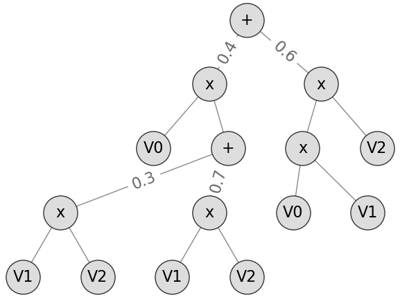
Figure 1: An SPN over three random variables V0, V1, and V2.

In order to encode a valid probability distribution, an SPN has to fulfill two structural requirements Poon and Domingos (2011). First, the scopes of the children of each product node need to be disjoint (decomposability). Second, the scopes of the children of each sum node need to be identical (completeness). In a valid SPN, the probability assigned to a given state $\bm{x}$ of the RVs $\bm{X}$ can be read out at the root node, and will be denoted $S(\bm{x})=P_{\bm{X}}(\bm{X}=\bm{x})$.

2.2 Probabilistic Inference within SPNs

Given an SPN $S$, $S(\bm{x})$ can be computed by evaluating the network bottom-up. When evaluating a leaf node $i$, $S_{i}(\mathbf{x}_{|\textsf{scope}(i)})$ corresponds to the probability of the state $\mathbf{x}_{|\textsf{scope}(i)}$ for the RV $\in\textsf{scope}(i)$: $S_{i}(\mathbf{x})=P_{\bm{X}_{|scope(i)}}(\bm{X}_{|\textsf{scope}(i)}=\mathbf{x}_{|\textsf{scope}(i)})$. The value of a product node corresponds to the product of its children values: $S_{i}(\bm{x}_{|\textsf{scope}(i)})=\prod_{i\rightarrow j\in S}S_{j}(\bm{x}_{|\textsf{scope}(j)})$; while, for a sum node its value corresponds to the weighted sum of its children values: $S_{i}(\bm{x}_{|\textsf{scope}(i)})=\sum_{i\rightarrow j\in S}w_{ij}S_{j}(\bm{x}_{|\textsf{scope}(j)})$.

All the marginal probabilities, the partition function, and even approximate MPE queries and states can be computed in time linear in the size of the network i.e. its number of edges as shown in Gens and Domingos (2013); Peharz (2015).

2.3 Structure Learning of SPNs

The prototypical structure learning algorithm for SPNs is LearnSPN Gens and Domingos (2013). It provides a simple greedy learning schema to infer both the structure and the parameters of an SPN from data. To this end, LearnSPN executes a greedy top-down structure search in the space of tree-shaped SPNs, i.e., networks in which each node has at most one parent, as summarized in Alg. 1.

Algorithm 1 LearnSPN($\mathcal{D}$, $\bm{X}$, $\mu$, $\rho$)

1:a set of samples $\mathcal{D}$ over RVs $\bm{X}$; $\mu$: minimum number of instances to split; $\rho$: statistical independence threshold

2:an SPN $S$ encoding a pdf over $\bm{X}$ learned from $\mathcal{D}$

3:if $|\bm{X}|=1$ then

4:     $S\leftarrow\mathsf{univariateDistribution}(\mathcal{D},\bm{X})$

5:else if $|\mathcal{D}|<\mu$ then

6:     $S\leftarrow\mathsf{fullFactorization}(\mathcal{D},\bm{X})$

7:else

8:     $\{\bm{X}_{d_{1}},\bm{X}_{d_{2}}\}\leftarrow\mathsf{splitFeatures}(\mathcal{D},\bm{X},\rho)$

9:     if $|\bm{X}_{d_{2}}|>0$ then

10:         $S\leftarrow\prod_{j=1}^{2}\mathsf{LearnSPN}(\mathcal{D},\bm{X}_{d_{j}},\mu,\rho)$

11:     else

12:         $\{\mathcal{D}_{i}\}_{i=1}^{R}\leftarrow\mathsf{clusterInstances}(\mathcal{D},\bm{X})$

13:         $S\leftarrow\sum_{i=1}^{R}\frac{|\mathcal{D}_{i}|}{|\mathcal{D}|}\mathsf{LearnSPN}(\mathcal{D}_{i},\bm{X},\mu,\rho)$      return $S$

Specifically, LearnSPN recursively partitions the training data matrix $\mathcal{D}$ consisting of i.i.d instances over $\bm{X}$, the set of columns, i.e., the RVs. For each call on a data slice, LearnSPN first tries to split the data slice by columns. This is done by splitting the current set of RVs into different groups such that the RVs in a group are statistically dependent while the groups are independent, i.e., the joint distribution factorizes over the groups of RVs. We denote this procedure as splitFeatures. If no independencies among features/RVs are found, i.e. the splitting fails, LearnSPN tries to cluster similar data slice rows (procedure clusterInstances) into groups of similar instances. In the original work of Gens and Domingos (2013), an online version of hard Expectation-Maximization (EM) algorithm is employed for this clustering step. Depending on the assumptions on the distribution of $\mathbf{X}$, other clustering and splitting algorithms may be more suitable and may be employed instead Vergari et al. (2015); Jaini et al. (2016); Molina et al. (2017, 2018). When a column split succeeds, LearnSPN adds a product node to the network whose children correspond to partitioned data slices. Similarly, after a row clustering step, it adds a sum node where children weights represent the proportions of instances falling into the obtained clusters. LearnSPN stops in two cases: (1) when the current data slice contains only one column or (2) when the number of its rows falls under a certain threshold $\mu$. In the first case, a leaf node, representing a univariate distribution, is introduced by a maximum likelihood estimation from the data slice. In the second case, the data slice’s RVs are modeled as a full factorization: they are assumed to be independent and a product node is put over a set of univariate leaf nodes (each of them estimated as described for the first case).

Indeed, clustering and splitting influence each other in terms of quality Vergari et al. (2015). If a good instance clustering is achieved then it is likely to enhance the variable splitting and the other way around. This also holds for more advanced structure learning approach beyond LearnSPN, too. For instance, Peharz et al. Peharz et al. (2013) introduced a bottom-up approach to learn SPN structures, using an information-bottleneck method. Vergari et al. Vergari et al. (2015) employed multivariate leaves for regularization. Adel et al. Adel et al. (2015) made use of efficient SVD-approaches. Rahman and Gogate Rahman and Gogate (2016) compressed tree-shaped structures into general DAGs. Jaini et al. Jaini et al. (2018) estimated product nodes via multi-view clustering over variables. Di Mauro et al. Di Mauro et al. (2018) investigated approximate independence testing, and Molina et al. Molina et al. (2018) non-parametric independence tests for learning SPN structures over hybrid domains. Rooshenas and Lowd Rooshenas and Lowd (2014) refined LearnSPN by learning leaf distributions using Markov networks represented by arithmetic circuits Lowd and Rooshenas (2013). The resulting SPN learner, called ID-SPN, is state-of-the-art in density estimation on binary data, when considering singleton models. Of course, any of the structure learning approaches can be improved by ensemble and boosting methods Liang et al. (2017); Di Mauro et al. (2017); Ramanan et al. (2019).

Algorithm 2 RSPF($\mathcal{D}$, $\bm{S}$)

1:a set of samples $\mathcal{D}$ over RVs $\bm{X}$; a set of input SPNs to be combined $\bm{S}=\mathcal{S}_{1},\dots,\mathcal{S}_{n}$

2:a $\mathit{RSPF}$ refining the input SPNs $\bm{S}$ on $\mathcal{D}$

3:$\mathit{RSPF}\leftarrow\sum_{i=1}^{n}\mathcal{S}_{i}/n$

4:$RSPF\leftarrow\mathsf{optimize}(\mathit{RSPF},\mathcal{D})$

5:return $\mathit{RSPF}$

3 Random Sum-Product Forests

While SPNs have attractive inference properties, scaling them in a manner similar to deep neural networks has proven challenging. The structural constraints which SPNs have to obey in order to guarantee validity are a major reason for this. They necessitate the careful design of structures, either by hand or through learning from data. Unfortunately, learning SPN structures (as sketched by LearnSPN) has proven hard to scale. This is mainly caused by the cost of determining how to split variables: Ideally, one would always determine the two subsets with minimum empirical mutual information. This takes cubic time, however Gens and Domingos (2013) and is thus much too slow. Therefore, one typically considers only pairwise dependencies in practice, reducing the cost to quadratic time, which is unfortunately still prohibitive for many applications. Recently, Peharz et al. Peharz et al. (2019) proposed random tensorized SPNs (RAT-SPNs), which forgo structure learning in favor of randomly generated structures.

Algorithm 3 ExtraSPN($\mathcal{D}$, $\bm{X}$, $\mu$, $\beta$)

1:a set of samples $\mathcal{D}$ over RVs $\bm{X}$; $\mu$: minimum number of instances to split; $\beta$: how likely the random feature splitting or random clustering could fail

2:an SPN $S$ encoding a pdf over $\bm{X}$ learned from $\mathcal{D}$

3:if $|\bm{X}|=1$ then

4:     $S\leftarrow\mathsf{univariateDistribution}(\mathcal{D},\bm{X})$

5:else if $|\mathcal{D}|<\mu$ then

6:     $S\leftarrow\mathsf{fullFactorization}(\mathcal{D},\bm{X})$

7:else

8:     $\{\bm{X}_{d_{1}},\bm{X}_{d_{2}}\}\leftarrow\mathsf{randomSplitFeatures}(\bm{X},\beta)$

9:     if $|\bm{X}_{d_{2}}|>0$ then

10:         $S\leftarrow\prod_{j=1}^{2}\mathsf{ExtraSPN}(\mathcal{D},\bm{X}_{d_{j}},\mu,\beta)$

11:     else

12:         $\{\mathcal{D}_{i}\}_{i=1}^{R}\leftarrow\mathsf{clusterInstances}(\mathcal{D},\bm{X})$ //or random

13:         $S\leftarrow\sum_{i=1}^{R}\frac{|\mathcal{D}_{i}|}{|\mathcal{D}|}\mathsf{ExtraSPN}(\mathcal{D}_{i},\bm{X},\mu,\beta)$      return $S$

While their approach of scaling random SPN structures yielded surprisingly good results, it carries the risk of introducing false independency assumptions. To repair such mistakes, we first propose an ensemble approach similar to Random Forests Breiman (2001), called Random Sum-Product Forests (RSPFs). As summarized in Alg. 2, it generates a number of individual SPNs which are then mixed together by adding a single sum node on top of the individual SPNs. This way, all mixed SPNs can be trained jointly using stochastic gradient or EM.

In principle, any SPN learned via structure learning (potentially in combination with bagging) or just RAT-SPNs can be used as components in this ensemble. Here, we opt for a faster and even simpler method: Akin to extremely randomized trees Geurts et al. (2006), each individual SPN is trained using the whole learning sample and the top-down splitting in LearnSPN is randomized, as summarized in Alg. 3. That is, instead of computing the locally optimal splitting of random variables based on, e.g., mutual information or independence tests, a random split is selected. The resulting extremely randomized SPNs (ExtraSPNs) are similar in spirit to extremely randomized cutset networks Di Mauro et al. (2017), except that ExtraSPNs do not use any statistical test for the splitting procedure. Instead, we fix a parameter $\beta$ to set the probability of the splitting test to fail, and randomly group the features in two clusters. In this way, the splitting procedure has constant complexity instead of the quadratic complexity of the G-test employed in the original LearnSPN. Moreover, to foster diversity in the set of ExtraSPNs, we sample the parameter $\mu$ at random from the range $[1,|\mathcal{D}|/\gamma]$ for each SPN. Here, $\mathcal{D}$ is the dataset and $\gamma$ is a hyperparameter that can shrink the range of the possible values of $\mu$. When $\gamma$ is not set to $1$ then the range of the possible values for $\mu$ is smaller, in this way we can both tune the learning times of the ExtraSPNs and also control their depth.

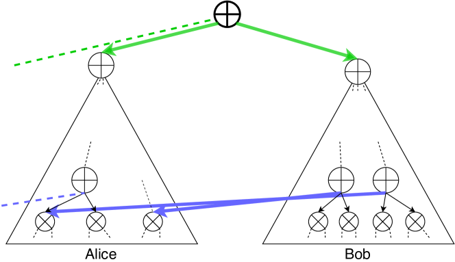
Figure 2: Illustration of Residual Sum-Product Learning. The blue edges denote residual links between the right (Bob) and left (Alice) SPN, which let Bob directly fit a residual. Green edges realize the global mixture to form a Sum-Product Random Forest.

4 Residual Sum-Product Learning

Random Sum-Product Forests suggest that learning ensembles of SPNs is as easy as mixing adding a single sum node at the top. Here, we aim to improve on this by making use of the fact that SPNs consist of highly specialized local substructures. This suggests that an ensemble method for SPNs should also work at the level of these substructures. Instead of hoping that each SPN fits a desired contribution to the global joint distribution, and inspired by ResNets He et al. (2016) and BoostResNet Huang et al. (2018), we explicitly let them fit residuals. Consider two SPNs called Alice and Bob as shown in Fig. 2. Our goal is to improve the performance of one of Bob’s sum nodes using a node $a(\bm{z})$ of the same scope from Alice. We denote Bob’s desired density as $b(\bm{z})$. Instead of learning this density directly, we instead let Bob fit a residual, namely, $r(\bm{z})=b(\bm{z})-a(\bm{z})$, up to proper weighting. That is, Bob’s original density is recast into $b(\bm{z})=a(\bm{z})+r(\bm{z})$, up to proper weighting. This can be achieved in a simple way: We add Alice’s product node as a child to Bob’s sum node, cf. 2. Adding such residual links between individual SPNs does not affect the validity of individual SPNs, since the scope of the two nodes is the same — the sum-product networks remain complete. For additional flexibility, we can also pick one of Alice’s nodes $a$ with scope($b$) $\subset$ scope($a$), and marginalize the surplus random variables from $a$ before adding the connection. The weights of the new mixture components can be set proportionally to their training data slices or eventually optimized jointly in a supplementary parameter estimation step, even after mixing Alice and Bob additionally using a single sum node at the top, such as in RSPFs. Thus, we propose to apply residual sum-product learning to every ExtraSPN within a RSPF. To do so, we generate an array of ExtraSPNs $E_{1},E_{2},\ldots,E_{n}$, pick a random one $E_{i}$, and introduce residual links between each pair $(E_{i},E_{j})$. We add a top sum node to form a RSPF and finally train all parameters jointly. We name the resulting model Residual SPNs (ResSPNs).

Overall, we hypothesize that it is easier to optimize the residual density than to optimize the original, unreferenced density. To the extreme, if a density from Alice was optimal, it would be easier to push the residual in Bob to zero than to fit the density in Bob from scratch or by mixing Alice and Bob at the top node only. As a result, we build a stronger density estimator by referencing to local context-specific substructures. In fact, residual connections make SPNs wider as also suggested by Fig. 2 and, in turn, increase the variance in sizes of training data slices used to train mixture components. This is akin to what is known for residual neural networks Veit et al. (2016) but now for hierarchical mixture models.

Different procedures are imaginable for selecting the pairs of nodes between which edges are to be added. For this reason, one can see the Residual Sum-Product Learning as a general schema, where different strategies for adding residual links may be selected based on the problem at hand. Here, we adopt a randomized greedy approach as summarized in Alg. 4. From the set of input SPNs, we randomly select one to which all future edges will be added. Then, we iteratively add references to each of the remaining input SPNs $S$, where the maximum percentage of nodes from which to draw connections to each one is given by the hyperparameter $k$. The connections are drawn in a greedy fashion: We start by selecting candidate nodes from our ResSPN by traversing it via breadth-first-search (BFS), excluding the root. For each visited node, we try to find a suitable partner in $S$, by also traversing it via BFS. If we find a suitable pairing, i.e. one where the scopes match as described above, we draw a residual link. This continues until either all pairs of nodes have been considered or the maximum number of connections has been drawn. Alternatively, one may also consider an informed variant where residual links are added only if they locally improve the learning objective on the training or a validation set. We name this variant InfoResSPN.

Algorithm 4 ResSPN($\mathcal{D}$, $\bm{S}$, $k$)

1:a set of samples $\mathcal{D}$; a set of input SPNs to be combined $\bm{S}=\mathcal{S}_{1},\dots,\mathcal{S}_{n}$; the ratio of nodes from which to draw residual links $k$

2:a $\mathit{ResSPN}$ built from $\bm{S}$ and optimized on $\mathcal{D}$

3:$\mathit{ResSPN}\leftarrow\textsf{copyRandomElement}(\bm{S})$

4:for $S\in\bm{S}\setminus\mathit{ResSPN}$ do

5:     $\eta=0$

6:     for $s_{1}\in$ BFS($\mathit{ResSPN}$) do

7:         for $s_{2}\in$ BFS($S$) do

8:              if scope($s_{1}$) $\subseteq$ scope($s_{2}$) then

9:                  $s_{2}^{\prime}\leftarrow$Marginalize($s_{2}$, scope$(s_{1})$)

10:                  Add connection from $s_{1}$ to $s_{2}^{\prime}$

11:                  $\eta\leftarrow\eta+1$                        

12:         if $\eta>k|\mathit{ResSPN}|$ then

13:              break               

14:$\mathit{ResSPN}\leftarrow\mathsf{RSPF}(\mathcal{D},\bm{S}\cup\{\mathit{ResSPN}\})$

15:return $\mathit{ResSPN}$

5 Experimental Evaluation

With our experimental evaluation, we aim to investigate whether the presented ensemble methods provide the intended benefits. In the process, we also explore how SPNs benefit from wider and deeper structures. Specifically, we examine the following questions:

(Q1)

Can RSPFs improve upon singleton SPNs learned by LearnSPN?

(Q2)

Can RSPFs repair wrong independencies?

(Q3)

Can residual links improve the performance of RSPFs?

(Q4)

Can informed residual links improve compared to non-informed ones?

To answer these questions, we learned a RSPF with and without residual links on standard benchmarks summarized in Tab. 1, split into training, validation and test sets. For parameter estimation we used the EM algorithm. The datasets are a subset of the ones used e.g. in Gens and Domingos (2013) and Rooshenas and Lowd (2014). They were firstly introduced in Lowd and Davis (2010) and in Haaren and Davis (2012). All of them are binary datasets and most of them are the binarized version of some popular datasets of the UCI machine learning repository Newman et al. (1998). All algorithms were implemented in Python making use of the SPFlow library Molina et al. (2019). All experiments were run on a DGX-2 system.

	$|\bm{X}|$	$|T_{train}|$	$|T_{val}|$	$|T_{test}|$
NLTCS	16	16181	2157	3236
MSNBC	17	291326	38843	58265
Plants	69	17412	2321	3482
Audio	100	15000	2000	3000
Jester	100	9000	1000	4116
Netflix	100	15000	2000	3000

Table 1: Statistics of the datasets used.

	Test Accuracy
	Baseline Singleton SPN Learners			Ensemble SPN
	Best ExtraSPN	LearnSPN	ID-SPN	RSPF	ResSPN
NLTCS	-6.153	-6.11	-6.02	-6.046$\Uparrow$	-6.040$\bullet$
MSNBC	-6.433	-6.11	-6.04	-6.104$\Uparrow$	-6.097$\bullet$
Plants	-16.683	-12.98	-12.54	-14.573$\uparrow$	-13.908$\bullet$
Audio	-42.639	-40.5	-39.79	-40.833$\uparrow$	-40.762$\bullet$
Jester	-55.335	-53.48	-52.86	-53.885$\uparrow$	-53.995$\uparrow$
Netflix	-60.330	-57.33	-56.36	-57.900$\uparrow$	-57.867$\bullet$

Table 2: Average test log-likelihood of RSPF and ResSPN compared to baseline singleton SPN learners. The best results including the baselines are shown in bold. As one can see, ID-SPN gives the best results, however, it uses Markov networks represented as ACs in the leaves. This can also be adapted for RSPFs. More importantly, ensembles of SPNs improve upon ExtraSPNs, as denoted by “$\uparrow$”, getting sometimes even better than LearnSPN, denoted as “$\Uparrow$”. Residual links can, in turn, improve the performance of RSPFs, as denoted by “$\bullet$”.

Training Accuracy
	RSPF	ResSPN
NLTCS	-6.006	-5.995$\bullet$
MSNBC	-6.097	-6.090$\bullet$
Plants	-14.056	-12.969$\bullet$
Audio	-39.784	-39.182$\bullet$
Jester	-52.352	-52.079$\bullet$
Netflix	-56.586	-55.982$\bullet$

Table 3: Average training log-likelihood of RSPF and ResSPN. The best results are denoted using “$\bullet$”. ResSPNs consistently achieve a better fit of the training data.

	Test Accuracy
	With Residual Links			Without Residual Links
	ResSPN 3	ResSPN 5	ResSPN 10	RSPF 3	RSPF 5	RSPF 10
NLTCS	-6.118$\bullet$	-6.068$\bullet$	-6.040$\bullet$	-6.192	-6.109	-6.046
MSNBC	-6.235$\bullet$	-6.145$\bullet$	-6.097$\bullet$	-6.316	-6.225	-6.104
Plants	-14.732$\bullet$	-14.631$\bullet$	-13.908$\bullet$	-15.616	-15.161	-14.573
Audio	-41.492$\bullet$	-41.433$\bullet$	-40.762$\bullet$	-41.883	-41.482	-40.833
Jester	-53.772$\bullet$	-54.040	-53.995	-53.987	-53.734$\bullet$	-53.885$\bullet$
Netflix	-58.609$\bullet$	-58.509$\bullet$	-57.867$\bullet$	-59.121	-58.570	-57.900
wins	6/6	5/6	5/6	0/6	1/6	1/6

Table 4: Average test log-likelihood of ResSPN — RSPF with residual links — for ensembles of 3, 5, and 10 ExtraSPNs compared to RSPFs without residual links. The best results are denoted using “$\bullet$”. Overall, one can clearly see that adding residual links is beneficial. The only exception is Jester, where ResSPNs overfit.

	Test Accuracy
	RSPF w/	InfoResSPN
	instance clustering
NLTCS	-6.064	-6.020$\bullet$
Audio	-41.919	-40.259 $\bullet$
Jester	-53.393	-53.214$\bullet$
Netflix	-59.668	-58.085$\bullet$

Table 5: Average test log-likelihood of InfoResSPN compared to RSPF based on ExtraSPNs with proper clustering. InfoResSPN improves (denoted with “$\bullet$”) the accuracy of the RSPF baseline. The regularization realized by InfoResSPN makes it less prone to overfitting (see Jester).

The following subsections will briefly describe the adopted experimental protocol and discuss the results for each question (Q1)-(Q4) in turn.

5.1 LearnSPN versus RSPFs – (Q1)

To answer (Q1), we build a RSPF from 10 ExtraSPNs. For learning the ExtraSPNs, we take the $\mu$ hyperparameter at random in the range $[1,|D|/5]$ and fix $\beta$ to 0.6. We similarly randomize the instance clustering step using the same hyperparameter $\beta$. The RSPF is then built as described in Alg. 2. We optimize the resulting structure with EM fixing a limit of 1000 iterations. The optimization stops if the variance of the training likelihood on the last 5 iterations is lower than 1e-7. Then, to assess the accuracy of learned estimators, we compute the average log-likelihood on the test sets. We compare it with the ones obtained with LearnSPN as reported in Rooshenas and Lowd (2014). Tab. 2 shows the average test likelihood for LearnSPN and RSPF. One can see that the ensemble strategy RSPF is competitive compared to LearnSPN since it can achieve similar accuracy and is more accurate on NLTCS and MSNBC without involving a meticulous hyperparameter selection. Thus, we can answer (Q1) positively: RSPFs improve upon singleton SPNs learned by LearnSPN.

5.2 Singleton ExtraSPNs versus RSPFs – (Q2)

Here, we consider the same RSPFs as before in the context of (Q1). We compare them with the single best available ExtraSPN. To do so, we generate a set of ExtraSPNs as before, except that we include a proper clustering step for generating sum nodes as opposed to random clustering. We then optimize their parameters with EM and report best test log-likelihood achieved among all of them. By looking at the results in Tab. 2, one can see that the RSPF always outperforms the best ExtraSPN. This means that as an ensemble method, RSPF does indeed improve upon its components, even when they are augmented using proper clustering and optimization. It also indicates that RSPF is able to repair false independency assumptions made by the ExtraSPNs. Therefore, we can affirmatively answer (Q2).

5.3 RSPFs with Residual Learning – (Q2, Q3)

Regarding these questions, we start from the same ExtaSPNs which were learned for (Q1) and (Q2), and use them to build ResSPNs, according to Alg. 4. We choose the number $n$ of ensemble components from $\{3,5,10\}$. After adding the residual links, we optimize the ResSPN structure on the training set with EM for a maximum number of 1000 iterations. We stop the optimization earlier if the variance of the training likelihood on the last 5 iterations is lower than 1e-07. We perform a hyperparameter search over $k$ within the range $[0.1,0.2]$, and select the models with the best accuracy on a separate validation set.

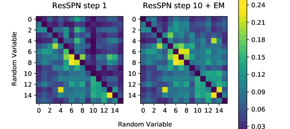
Figure 3: The lower triangle of the matrices shows the pairwise empirical mutual information between variables in the NLCTS dataset. (Upper triangle, left) MI computed with a ResSPN after adding links to one other SPN. (Upper triangle, right) MI computed with a ResSPN after adding links to 9 other SPNs and optimizing with EM for 10 iterations. The fact that the MI of the fully trained ResSPN is much closer to the empirical MI indicates that ResSPNs are able to repair wrong independence assumptions.

Tab. 2 summarizes the average test log-likelihood of ResSPNs and RSPFs. As one can clearly see, residual links generally improve the test accuracy, with Jester being the only exception. To investigate the possibility of overfitting, we also analyzed the training likelihood of both models as reported in Tab. 3. One can observe that on all datasets including Jester, the ResSPN indeed achieves a better training accuracy, indicating that overfitting did indeed occur on Jester. The dataset appears to be generally prone to overfitting, as even for RSPFs, better results are achieved with fewer than 10 ensemble components (Tab. 4). In summary, residual links improve the ability of the model to fit the training data and they generally also yield a better test accuracy. These observations also hold when a smaller number of ExtraSPNs are used, as can be seen in Tab. 4. Given this, we can positively answer (Q3): residual links indeed improve the performance of RSPFs.

Additionally, ResSPNs are also capable of repairing wrong independence assumptions made by the singleton models (Q2). To demonstrate this, we compare the empirical pairwise mutual information between random variables on the training dataset with the one computed on our model at various stages of training. Fig. 3 depicts the empirical pairwise mutual information on the NLTCS dataset on the lower triangle of the matrices, and the mutual information computed from our model on the upper triangle. The left matrix uses a ResSPN in the early stages of training, after the first set of residual links has been added, while the right one shows the result for a fully trained ResSPN based on 10 ExtraSPNs. It is apparent that after full training, the ResSPN is much more capable of representing the correlations among the random variables, since the matrix on the right is almost symmetric.

	LearnSPN		ResSPN 10
	edges	layers	edges	layers
NLTCS	7509	4	17102	169
MSNBC	22350	4	8040	136
Plants	55668	6	66498	298
Audio	70036	8	153791	296
Jester	36528	4	104053	259
Netflix	17742	4	153791	296

Table 6: The structure of ResSPNs can be deeper and/or wider compared to singleton tree-SPNs learned via LearnSPN as reported in Vergari et al. (2015).

5.4 Regularization via informed residual – (Q4)

Finally, we investigate whether using an informed strategy for adding residual links and, hence, reducing the level of greediness can be beneficial in terms of model accuracy. To this end, we explore a variant of ResSPNs called InfoResSPN, which takes advantage of the information provided by input SPNs learned via LearnSPN and its derivatives. Specifically, we modify line 6 in Alg. 4 such that residual links are only added if they improve the model’s training likelihood on the data slice for which the node $s_{1}$ is responsible for according to LearnSPN.

Tab. 5 summarizes the results, comparing InfoResSPN and RSPF. In order to get a more challenging baseline, this time RSPFs are composed of ExtraSPNs learned with regular instance clustering instead of random clustering. We opt for this stronger baseline since we want to check whether informed residual links can be successful at extracting the knowledge contained in each of the ExtraSPNs. We fix the ratio of candidate nodes for each iteration to $k=0.1$, and use 10 ExtraSPNs on NLTCS and Audio and 5 for the other datasets. All the models were optimized with EM for 10 iterations on the training set.

InfoResSPNs improve upon the RSPF baseline. Moreover, InfoResSPN also achieves overall better accuracy than ResSPN, and even succeeds on Jester where ResSPN overfitted. Intuitively, InfoResSPN is less prone to overfitting since its strategy for adding residual links is stricter compared to ResSPNs. Thus, we can positively answer to question (Q4): employing informed residual links, even if it adds a computational burden, improves the accuracy of learned models and may help make them less prone to overfitting.

5.5 Discussion of the Experimental Results

We addressed the questions (Q1)-(Q4) in order to answer a more general question, namely, whether deeper and wider probabilistic models are actually beneficial. It is well known that learning and scaling deep architectures is a challenging problem, and SPNs face this challenge too. We already discussed the results in terms of accuracy in the previous sections, thus, taking into account the structural details of the learned models shown in Tab. 6, we can indeed confirm that wider and deeper SPNs —learned by adding residual links— in general, perform considerably better than singleton tree-shaped models. With ResSPNs, it is possible to obtain results competitive to LearnSPN without the need for expensive hyperparameter selection as well as costly statistical independence tests and clustering. In Tab. 2 one can also see that performance in accuracy is comparable to ID-SPN, which is the most accurate method so far while also being difficult to scale due to the learning of Markov Networks as multivariate leaves and the need of an attentive hyperparameter selection. In contrast, RSPF and ResSPNs naturally scale to thousands of random variables. In any case, one can, of course, employ ID-SPNs instead of ExtraSPNs within RSFPs — they are orthogonal to each other. Doing so provides an interesting avenue for future work. This also highlights the peculiarity of ResSPN that can be seen as a general schema: One can easily extend and plug-in different singleton learners, employ different strategies for adding residual links, and make use of many deep neural learning techniques.

6 Conclusion

Deeper and wider probabilistic models are more difficult to train. To make this task easier, we have introduced an ensemble learning framework for sum-product networks (SPNs), which makes it possible to combine arbitrary groups of SPNs into a larger model. Our experimental evidence shows that even when the input SPNs are generated randomly, the resulting random sum-product forests (RSPFs) are competitive with state of the art SPN learners. As it turns out, ensembles of random SPNs can indeed “repair” wrong independence assumptions made by individual SPNs. As an additional improvement to RSPFs, we have proposed residual links to substructures in other SPNs, yielding ResSPNs.

RSPNs and ResSPNs can be seen as general schemas for building ensembles of SPNs and thus provide several interesting avenues for future work. One is to explore different structure learners instead of ExtraSPN or even a mix of different ones. Furthermore, one should explore other strategies for adding residual links. For instance, given that we have a tractable model at hand, one may compute the expected value of adding a residual link. Post-pruning the final ResSPN, employing dropout as well as online learning are further interesting avenues. Of course, one should run more experiments, i.e., on images, text, and hybrid domains. Most important, however, is to push the merge of deep probabilistic and neural learning further that Stelzner et al. Stelzner et al. (2019) have already shown to be beneficial.

References

- Adel et al. [2015] Tameem Adel, David Balduzzi, and Ali Ghodsi. Learning the structure of sum-product networks via an svd-based algorithm. In Proceedings of UAI, 2015.
- Amer and Todorovic [2015] Mohamed Amer and Sinisa Todorovic. Sum product networks for activity recognition. IEEE Transactions on Pattern Analysis and Machine Intelligence, 2015.
- Breiman [2001] Leo Breiman. Random forests. Machine Learning, 45(1):5–32, 2001.
- Chechetka and Guestrin [2008] Anton Chechetka and Carlos Guestrin. Efficient principled learning of thin junction trees. In Proceedings of NIPS, pages 273–280. 2008.
- Cheng et al. [2014] Wei-Chen Cheng, Stanley Kok, Hoai Vu Pham, Hai Leong Chieu, and Kian Ming Adam Chai. Language modeling with Sum-Product Networks. In Proceedings of INTERSPEECH, pages 2098–2102, 2014.
- Di Mauro et al. [2017] N. Di Mauro, A. Vergari, T. Basile, and F. Esposito. Fast and accurate density estimation with extremely randomized cutset networks. In Proceedings of ECML/PKDD, pages 203–219, 2017.
- Di Mauro et al. [2018] Nicola Di Mauro, Floriana Esposito, Fabrizio G. Ventola, and Antonio Vergari. Sum-product network structure learning by efficient product nodes discovery. Intelligenza Artificiale, 12(2):143–159, 2018.
- Dinh et al. [2016] L. Dinh, J. Sohl-Dickstein, and S. Bengio. Density estimation using real NVP. arXiv preprint arXiv:1605.08803, 2016.
- Gens and Domingos [2013] Robert Gens and Pedro Domingos. Learning the Structure of Sum-Product Networks. In Proceedings of the ICML, pages 873–880, 2013.
- Geurts et al. [2006] Pierre Geurts, Damien Ernst, and Louis Wehenkel. Extremely randomized trees. Machine Learning, 63(1):3–42, 2006.
- Goodfellow et al. [2014] I. J. Goodfellow, J. Pouget-Abadie, M. Mirza, B. Xu, D. Warde-Farley, S. Ozair, A. Courville, and Y. Bengio. Generative adversarial nets. In Proceedings of NIPS, pages 2672–2680, 2014.
- Haaren and Davis [2012] Jan Van Haaren and Jesse Davis. Markov network structure learning: A randomized feature generation approach. In Proceedings of AAAI, 2012.
- He et al. [2016] Kaiming He, Xiangyu Zhang, Shaoqing Ren, and Jian Sun. Deep residual learning for image recognition. In Proceedings of CVPR, pages 770–778, 2016.
- Hoffman [2017] Matthew D. Hoffman. Learning deep latent Gaussian models with Markov chain Monte Carlo. In Proceedings of ICML, pages 1510–1519, 2017.
- Huang et al. [2018] Furong Huang, Jordan Ash, John Langford, and Robert Schapire. Learning deep ResNet blocks sequentially using boosting theory. In Proceedings of ICML, pages 2058–2067, 2018.
- Jaini et al. [2016] Priyank Jaini, Abdullah Rashwan, Han Zhao, Yue Liu, Ershad Banijamali, Zhitang Chen, and Pascal Poupart. Online algorithms for sum-product networks with continuous variables. In Proceedings of PGMs, 2016.
- Jaini et al. [2018] P. Jaini, A. Ghose, and P. Poupart. Prometheus: Directly learning acyclic directed graph structures for sum-product networks. In Proceedings of PGM, 2018.
- Kingma and Dhariwal [2018] D. P. Kingma and P. Dhariwal. Glow: Generative flow with invertible 1x1 convolutions. In Proceedings of NIPS, pages 10236–10245, 2018.
- Kingma and Welling [2014] D. P. Kingma and M. Welling. Auto-encoding variational Bayes. In Proceedings of ICLR, 2014.
- Larochelle and Murray [2011] Hugo Larochelle and Iain Murray. The Neural Autoregressive Distribution Estimator. In Proceedings of AISTATS, pages 29–37, 2011.
- Liang et al. [2017] Y. Liang, J. Bekker, and G. Van den Broeck. Learning the structure of probabilistic sentential decision diagrams. In Proceedings of UAI, 2017.
- Lowd and Davis [2010] Daniel Lowd and Jesse Davis. Learning Markov network structure with decision trees. In Proceedings of IEEE ICDM, pages 334–343, 2010.
- Lowd and Rooshenas [2013] Daniel Lowd and Amirmohammad Rooshenas. Learning Markov networks with arithmetic circuits. In Proceedings of AISTATS, pages 406–414, 2013.
- Molina et al. [2017] Alejandro Molina, Sriraam Natarajan, and Kristian Kersting. Poisson sum-product networks: A deep architecture for tractable multivariate poisson distributions. In Proceedings of AAAI, 2017.
- Molina et al. [2018] Alejandro Molina, Antonio Vergari, Nicola Di Mauro, Sriraam Natarajan, Floriana Esposito, and Kristian Kersting. Mixed sum-product networks: A deep architecture for hybrid domains. In Proceedings of AAAI, pages 3828–3835, 2018.
- Molina et al. [2019] Alejandro Molina, Antonio Vergari, Karl Stelzner, Robert Peharz, Pranav Subramani, Nicola Di Mauro, Pascal Poupart, and Kristian Kersting. Spflow: An easy and extensible library for deep probabilistic learning using sum-product networks. CoRR, abs/1901.03704, 2019.
- Newman et al. [1998] C.L. Newman, Blake D.J., and C.J. Merz. UCI repository of machine learning databases, 1998.
- Peharz et al. [2013] Robert Peharz, Bernhard Geiger, and Franz Pernkopf. Greedy Part-Wise Learning of Sum-Product Networks. In Proceedings of ECML-PKDD, 2013.
- Peharz et al. [2014] Robert Peharz, Georg Kapeller, Pejman Mowlaee, and Franz Pernkopf. Modeling speech with sum-product networks: Application to bandwidth extension. In Proceedings of ICASSP, 2014.
- Peharz et al. [2019] Robert Peharz, Antonio Vergari, Karl Stelzner, Alejandro Molina, Martin Trapp, Kristian Kersting, and Zoubin Ghahramani. Random Sum-Product Networks: A Simple and Effective Approach to Probabilistic Deep Learning. Proceedings of UAI, 2019.
- Peharz [2015] Robert Peharz. Foundations of Sum-Product Networks for Probabilistic Modeling. PhD thesis, Graz University of Technology, SPSC, 2015.
- Poon and Domingos [2011] Hoifung Poon and Pedro Domingos. Sum-Product Networks: a New Deep Architecture. Proceedings of UAI, 2011.
- Rahman and Gogate [2016] Tahrima Rahman and Vibhav Gogate. Merging strategies for sum-product networks: From trees to graphs. In Proceedings of UAI, 2016.
- Ramanan et al. [2019] Nandini Ramanan, Mayukh Das, Kristian Kersting, and Sriraam Natarajan. Discriminative non-parametric learning of arithmetic circuits. In Working Notes of the ICML Workshop on Tractable Probabilistic Models (TPM). 2019.
- Ranganath et al. [2014] Rajesh Ranganath, Sean Gerrish, and David Blei. Black box variational inference. In Proceedings of AISTATS, pages 814–822, 2014.
- Ratajczak et al. [2014] Martin Ratajczak, S Tschiatschek, and F Pernkopf. Sum-product networks for structured prediction: Context-specific deep conditional random fields. Proceedings of the ICML Workshop on Learning Tractable Probabilistic Models, pages 1–10, 2014.
- Rezende et al. [2014] D. J. Rezende, S. Mohamed, and D. Wierstra. Stochastic backpropagation and approximate inference in deep generative models. In Proceedings of ICML, pages 1278–1286, 2014.
- Rooshenas and Lowd [2014] Amirmohammad Rooshenas and Daniel Lowd. Learning Sum-Product Networks with Direct and Indirect Variable Interactions. In Proceedings of ICML, 2014.
- Stelzner et al. [2019] Karl Stelzner, Robert Peharz, and Kristian Kersting. Faster attend-infer-repeat with tractable probabilistic models. In Proceedings of ICML, 2019.
- van den Oord et al. [2016a] A. van den Oord, N. Kalchbrenner, L. Espeholt, O. Vinyals, A. Graves, et al. Conditional image generation with pixelcnn decoders. In Proceedings of NIPS, pages 4790–4798, 2016.
- van den Oord et al. [2016b] A. van den Oord, N. Kalchbrenner, and K. Kavukcuoglu. Pixel recurrent neural networks. In Proceedings of ICML, pages 1747–1756, 2016.
- Veit et al. [2016] Andreas Veit, Michael J. Wilber, and Serge J. Belongie. Residual networks behave like ensembles of relatively shallow networks. In Proceedings of NIPS, pages 550–558, 2016.
- Vergari et al. [2015] Antonio Vergari, Nicola Di Mauro, and Floriana Esposito. Simplifying, Regularizing and Strengthening Sum-Product Network Structure Learning. In Proceedings of ECML-PKDD, 2015.
- Yuan et al. [2016] Zehuan Yuan, Hao Wang, Limin Wang, Tong Lu, Shivakumara Palaiahnakote, and Chew Lim Tan. Modeling spatial layout for scene image understanding via a novel multiscale sum-product network. Proceedings of Expert Systems with Applications, 63:231 – 240, 2016.