Impacts into rotating targets: angular momentum draining and efficient formation of synthetic families

About 10% of the observed asteroids have rotational periods lower than $P=3\,\rm h$ and they seem to be relatively close to the spin barrier. Yet, the rotation has often been neglected in simulations of asteroid collisions. To determine the effect of rotation, we perform a large number of SPH/N-body impact simulations with rotating targets. We developed a new unified SPH/N-body code with self-gravity, suitable for simulations of both fragmentation phase and gravitational reaccumulation. The code has been verified against previous ones (Benz and Asphaug, 1994), but we also tested new features, e.g. rotational stability, tensile stability, etc. Using the new code, we ran simulations with $D_{\rm pb}=10\,\rm km$ and $100\,\rm km$ monolithic targets and compared synthetic asteroid families created by these impacts with families corresponding to non-rotating targets. The rotation affects mostly cratering events at oblique impact angles. The total mass ejected by these collision can be up to five times larger for rotating targets. We further compute the transfer of the angular momentum and determine conditions under which impacts accelerate or decelerate the target. While individual cratering collisions can cause both acceleration and deceleration, the deceleration prevails on average, collisions thus cause a systematic spin-down of asteroid population.

1 Asteroid collisions in the Main Belt

The Main Belt of asteroids is a collisional system. The breakups of asteroids have been recorded in the form of asteroid families (Nesvorný et al., 2015; Vinogradova, 2019), we can also see impact features, such as craters or boulders, on surfaces of asteroids. These features can be observed directly during a satellite flyby or even with ground-based instruments (Vernazza et al., 2018; Fétick et al., 2019).

Physical processes during asteroid collisions are rather complicated for purely analytical estimates to yield precise quantitative results; it is necessary to model a propagation of shock wave in the target, crack growth and consequent fragmentation, gravitational reaccumulation of ejected fragments, etc. Fragmentation of targets due to hyper-velocity impacts has been studied using laboratory experiments (Nakamura and Fujiwara, 1991; Morris and Burchell, 2017; Wickham-Eade et al., 2018). While the experiments can produce valuable constraints, the results cannot be directly compared with the breakups of asteroids, as the sizes of targets and kinetic energies of the impact would have to be extrapolated over several orders of magnitude. Experiments also do not take into account a gravitational reaccumulation. The collisions of asteroids are therefore commonly studied using numerical methods; the experiments then provide the calibration for the respective numerical codes.

Common methods for studying the collisions can be divided into particle-based (for example the N-body code pkdgrav, see Richardson et al., 2000), and shock-physics ones, such as mesh-based methods (used by code iSALE, see Suetsugu et al., 2018) or the smoothed particle hydrodynamics (Jutzi et al., 2015), used in this work. This is a Lagrangian, grid-less method, which makes it suitable for impact simulations, as the computational domain is not a priori known. Especially in a hit-and-run impact, fragments of the projectile can travel to considerable distances from the target. In SPH, the distant fragments do not require any special handling (they only might affect the performance of the code). SPH is also versatile, allowing to relatively easily implement new physics. The model of fragmentation can be straightforwardly incorporated into SPH, but it would be a difficult task for grid-based methods.

An outcome of a collision depends on a number of parameters, namely the diameter $D_{\rm pb}$ of the target, the diameter $d_{\rm imp}$ of the projectile, the specific impact energy $Q$, the impact angle $\phi_{\rm imp}$, but also the rotational periods of the colliding bodies, their shapes, material properties, etc. For completeness, we should also include parameters introduced by the numerical scheme, such as the spatial resolution, the time step, the artificial viscosity $\Pi_{\rm AV}$, etc. The extent of this parameter space prohibits a thorough analysis of every collision as a function of all the mentioned parameters, we thus have to restrict ourselves to a particular set of simulations, varying some parameters and keeping the others constant.

Asteroidal targets have been considered non-rotating in most previous studies of asteroid families (Durda et al., 2007; Benavidez et al., 2012; Ševeček et al., 2017; Benavidez et al., 2018; Jutzi et al., 2019). Jutzi et al. (2013) considered a rotating Vesta, rotating bodies have also been studied by Jutzi and Benz (2017). Ćuk and Stewart (2012) and Canup (2008) take the rotation into account for simulations of the Moon-forming impact, Canup (2005) for the impact event forming Pluto and Charon. Ballouz et al. (2015) used an N-body code to simulate collisions of rotating rubble-pile asteroids, Takeda and Ohtsuki (2007, 2009) studied the angular momentum transfer for both stationary and rotating rubble-piles. In this work, we study a formation of asteroid families from monolithic targets, extending the parameters of the simulation by the initial rotational period $P_{\rm pb}$ of the target, including cases close to the spin barrier.

The paper is organized as follows. In Section 2, we describe our numerical model. Section 3 analyzes differences between synthetic families created from parent bodies with various rotational periods. Section 4 is focused on largest remnants, specifically on their accelerations or decelerations and the angular momentum transfer. Finally, we summarize our results in Section 5.

2 Numerical model

We developed a new SPH/N-body code. The code is publicly available, see Appendix C. In this section, we do not attempt to present a thorough review of the SPH method (as e.g. Cossins, 2010), but instead we summarize the exact equations used in the code, emphasizing the modifications introduced in order to properly deal with rotating bodies.

2.1 Set of equations

The set of hydrodynamical equations is solved with a smoothed particle hydrodynamics (Monaghan, 1985). The continuum is discretized into particles co-moving with the continuum, with the density profile of the particles given by a kernel $W$, which is a cubic spline in our case:

$$W(r,h)=\frac{\sigma}{h^{3}}\left\{\begin{array}[]{ll}\frac{1}{4}(2-q)^{3}-(1-q)^{3}\,,&0\leq q<1\,,\\ \frac{1}{4}(2-q)^{3}\,,&1\leq q<2\,,\\ 0&q\geq 2\,,\end{array}\right.$$ (1)

where $q\equiv r/h$.

Below, we denote indices of particles with Latin subscripts (usually $i$, $j$, …), the components of vector and tensor quantities with Greek superscripts (usually $\alpha$, $\beta$, …). We also use Einstein notation to sum over components (but not for particles, of course).

The equation of motion for $i$-th particle reads:

$$\frac{{\rm d}v_{i}^{\alpha}}{{\rm d}t}=\sum_{j}m_{j}\left(\frac{\sigma^{\alpha\beta}_{i}}{\rho_{i}^{2}}+\frac{\sigma^{\alpha\beta}_{j}}{\rho_{j}^{2}}+\Pi_{ij}\delta^{\alpha\beta}+\zeta^{\alpha\beta}_{ij}f^{n}\right)\frac{\partial W_{ij}}{\partial x^{\beta}}+\\ +\nabla\Phi-\left[\bm{\omega}\times(\bm{\omega}\times\bm{r}_{i})\right]^{\alpha}-\left[2\bm{\omega}\times\bm{v}_{i}\right]^{\alpha}\,,$$ (2)

where $\sigma^{\alpha\beta}=-P\delta^{\alpha\beta}+S^{\alpha\beta}$ is the total stress tensor, $\Pi$ is the artificial viscosity (Monaghan and Gingold, 1983), $\zeta^{\alpha\beta}f^{n}$ is the artificial stress (Monaghan, 2000), $\Phi$ is the gravitational potential (including both external fields and self-gravity of particles), and $\bm{\omega}$ is the angular velocity of the reference frame.

The respective terms in the Eq. (2) correspond to the stress divergence, gravitational acceleration, centrifugal force and Coriolis force. Inertial forces are only applied if the simulation is carried out in a non-inertial reference frame, corotating with the target asteroid (see Appendix B).

We use the standard artificial viscosity with linear and quadratic velocity divergence terms and coefficients $\alpha_{\rm AV}$ and $\beta_{\rm AV}$, respectively. This term is essential for a proper shock propagation and thus is always enabled in our simulations. Optionally, it is possible to enable the Balsara switch (Balsara, 1995), which reduces the artificial viscosity in shear motions in order to reduce an unphysical angular momentum transfer. Additionally, the code includes the artificial stress term $\zeta^{\alpha\beta}f^{n}$, which reduces the tensile instability, i.e. an unphysical clustering of particles due to negative pressure. We tested the effects of this term using the “colliding rubber cylinders” test (c.f. Schäfer et al., 2016).

We use a different discretization of the equation than in Ševeček et al. (2017), as we found the above equation to be more robust, avoiding a high-frequency oscillation in the pressure field. This is a recurring problem in high-velocity impact simulations and while it can be suppressed by a larger kernel support, additional modifications of the method have been suggested to address the issue, for example the $\delta$-SPH modification (Marrone et al., 2011).

The density is evolved using the continuity equation:

$$\frac{{\rm d}\rho_{i}}{{\rm d}t}=\sum_{j}m_{j}\frac{\partial v_{i}^{\alpha}}{\partial x^{\alpha}}\,.$$ (3)

We solve the evolution equation instead of direct summation of particle masses to avoid the artificial low-density layer at the surface of the asteroid (Reinhardt and Stadel, 2017). The velocity gradient at the right-hand side of Eq. (3) is computed as:

$$\rho_{i}\frac{\partial v_{i}^{\alpha}}{\partial x^{\beta}}=\sum_{j}m_{j}(v_{j}^{\alpha}-v_{i}^{\alpha})\,C_{i}^{\beta\gamma}\frac{\partial W_{ij}}{\partial x^{\gamma}}\,,$$ (4)

where the correction tensor $C^{\alpha\beta}$ is defined as (Schäfer et al., 2016):

$$C_{i}^{\alpha\beta}\equiv\left[\sum_{j}\frac{m_{j}}{\rho_{j}}(r_{j}^{\alpha}-r_{i}^{\alpha})\frac{\partial W_{ij}}{\partial x^{\beta}}\right]^{-1}\,.$$ (5)

In case the bracketed matrix is not invertible, we use the Moore-Penrose pseudo-inverse instead. The correction tensor is further set to 1 for fully damaged material.

The correction tensor has been introduced to tackle the linear inconsistency of the standard SPH formulation. It is a fundamental term in the velocity gradient that allows for a stable bulk rotation of the simulated body and significantly improves the conservation of the total angular momentum.

We evolve the internal energy $u$ using the energy equation:

$${{\rm d}u_{i}\over{\rm d}t}=-{\sigma^{\alpha\beta}\over\rho_{i}}\frac{\partial v_{i}^{\alpha}}{\partial x^{\beta}}+\sum_{j}\frac{1}{2}m_{j}\Pi_{ij}(v^{\alpha}_{i}-v_{j}^{\alpha})\frac{\partial W_{ij}}{\partial x^{\alpha}}+\\ \sum_{j}\frac{1}{2}m_{j}\zeta^{\alpha\beta}_{ij}f^{n}(v^{\beta}_{i}-v_{j}^{\beta})\frac{\partial W_{ij}}{\partial x^{\alpha}}\,.$$ (6)

In this equation the velocity gradient is also corrected by the tensor $C^{\alpha\beta}$. While this is required for a consistent handling of rotation, the inequality of kernel gradients used in the energy equation (6) and in the equation of motion (2) implies the total energy is generally not conserved in the simulations. This is usually not an issue, as the total energy does not increase by more than 5%.

However, in some cases (weak cratering impacts or exceedingly long integration time), the energy growth can be prohibitive. For such cases, the code also offers an alternative way to evolve the internal energy, using a compatibly-differenced scheme (Owen, 2014). Instead of computing the energy derivative, the energy change is computed directly from particle pair-wise accelerations $a_{ij}^{\alpha}$ and half-step velocities $w_{i}^{\alpha}=v_{i}^{\alpha}+\frac{1}{2}a_{i}^{\alpha}\Delta t$, using the equation:

$$\Delta u_{i}=\sum_{j}f_{ij}(w_{j}^{\alpha}-w_{j}^{\beta})\,a_{ij}^{\alpha}\Delta t\,,$$ (7)

where the energy partitioning factors $f_{ij}$ can be chosen arbitrarily, provided they fulfil constraint $f_{ij}+f_{ji}=1$. With this form of SPH, the total energy can be conserved to machine precision, at a cost of performance overhead. However, this does not solve the inconsistency mentioned above.

The listed set of equations is supplemented by the Tillotson equation of state (Tillotson, 1962). To close the set of equation, we have to specify the constitutive equation. We use the Hooke’s law, evolving the deviatoric stress tensor in time using:

$${{\rm d}S^{\alpha\beta}_{i}\over{\rm d}t}=2\mu\left(\frac{\partial v_{i}^{\alpha}}{\partial x^{\beta}}-{{1\over 3}}\delta^{\alpha\beta}\frac{\partial v_{i}^{\gamma}}{\partial x^{\gamma}}\right)\,,$$ (8)

where $\mu$ denotes the shear modulus. To account for plasticity of the material, we further use the von Mises criterion, which reduces the deviatoric stress tensor by the factor:

$$f=\operatorname{min}\left[\frac{Y_{0}^{2}(1-u/u_{\rm melt})^{2}}{\frac{3}{2}S^{\alpha\beta}S^{\alpha\beta}},1\right]\,,$$ (9)

where $Y_{0}$ is the yield stress and $u_{\rm melt}$ is the specific melting energy. While more complex, pressure-dependent rheology models exist (Jutzi et al., 2015), von Mises rheology is reasonable for monolithic asteroids and still consistent with laboratory experiments (Remington et al., 2018). The effects of friction have been studied by Jutzi et al. (2015) or Kurosawa and Genda (2018); and we do not discuss such effect in this work.

Additionally, we integrate the fragmentation model to model an activation of flaws and a propagation of fractures in the material. Following Benz and Asphaug (1994), we define a scalar quantity damage $D$, modifying the total stress tensor as

$$\sigma_{D}^{\alpha\beta}=-\left(1-DH(-P)\right)P\delta^{\alpha\beta}+(1-D)S^{\alpha\beta}\,,$$ (10)

where $H(x)$ is the Heaviside step function. A fully damaged material ($D=1$) has no shear nor tensile strength, it only resists to compressions.

Smoothing lengths of particles are evolved to balance the changes of particle concentration. We thus derive the equation directly from the continuity equation:

$$\frac{{\rm d}h_{i}}{{\rm d}t}=\frac{h_{i}}{3}\frac{\partial v_{i}^{\alpha}}{\partial x^{\alpha}}\,.$$ (11)

Since it is also an evolution equation, we need to specify the initial conditions for smoothing lengths:

$$h=\eta\left(\frac{V}{N}\right)^{\frac{1}{3}}\,,$$ (12)

where $V$ is the volume of the body, $N$ is the number of particles in the body and $\eta$ is a free non-dimensional parameter, which we set to $\eta=1.3$, corresponding to an average number of neighbouring particles $N_{\rm neigh}\simeq 65$.

2.2 Gravity

Beside hydrodynamics, the code also computes accelerations of SPH particles due to self-gravity. To compute it efficiently (albeit approximately), we employ the Barnes-Hut algorithm (Barnes and Hut, 1986). Instead of computing pair-wise interactions of particles, we first cluster the particles hierarchically and evaluate gravitational moments of particles in each node of the constructed tree. The accelerations are then computed by a tree-walk; if the evaluated node is distant enough, the acceleration can be approximated by evaluating the multipole moments up to the octupole order, otherwise we descend into child nodes. The precision of the method is controlled by an opening radius $r_{\rm open}$. For an extensive description of the method, see Stadel (2001).

As our SPH particles are spherically symmetric, they can be replaced by point masses, provided they do not intersect each other (the corresponding kernel $W_{ij}$ is zero). However, it is absolutely necessary to account for softening of the gravitational potential for neighbouring particles. We follow Cossins (2010) by introducing a gravitational softening kernel $\phi$ (associated with the SPH smoothing kernel $W$) using the equation:

$$\frac{\partial\phi}{\partial r}=\frac{4\pi}{r}\int\limits_{0}^{r}r^{\prime 2}W(r^{\prime})\,{\rm d}r^{\prime}+\frac{h}{r^{2}}\,.$$ (13)

The gravitational kernel $\phi$ corresponding to our M4 spline kernel $W$ is then:

$$\phi(r,h)=\left\{\begin{array}[]{ll}\frac{2}{3}q^{2}-\frac{3}{10}q^{4}+\frac{1}{10}q^{5}-\frac{7}{5}\,,&0\leq q<1\,,\\ \frac{4}{3}q^{2}-q^{3}+\frac{3}{10}q^{4}-\frac{1}{10}q^{5}\\ \hskip 50.0pt-\frac{8}{5}+\frac{1}{15q}\,,&1\leq q<2\,,\\ -\frac{1}{q}\,,&q\geq 2\,,\end{array}\right.$$ (14)

where $q\equiv r/h$. This kernel does not have a compact support, though.

2.3 Temporal discretization

Using derivatives computed at each time step, the equations are integrated using explicit timestepping. The scheme used in this work is the predictor-corrector, however other schemes are implemented in the code, such as the leapfrog, 4th order Runge-Kutta or Bulirsch-Stoer.

The value of the time step is determined by the CFL criterion:

$$\Delta t\leq C_{\rm CFL}\min_{i}\frac{h_{i}}{c_{\rm s}}\,,$$ (15)

where $h_{i}$ is the smoothing length of $i$-th particle, $c_{\rm s}$ the local sound speed and $C_{\rm CFL}$ is the Courant number. In our simulations, we usually use $C_{\rm CFL}=0.25$, as higher values can lead to instabilities in some cases. Moreover, we restrict the time step by the value-to-derivative ratio of all time-dependent quantities in the simulation to control the discretization errors. The upper limit of the time step is therefore:

$$\Delta t\leq C_{\rm d}\frac{|x|+s_{x}}{|\dot{x}|}\,,$$ (16)

where $s_{x}$ is a parameter with the same dimensions as $x$, assigned to each quantity in order to avoid zero time step if the quantity $x$ is zero. Constant $C_{\rm d}$ is 0.2 for all quantities.

2.4 Equilibrium initial conditions

Setting up the initial conditions for the impact simulation is not a trivial task. It is necessary to assign a particular value of the density $\rho$, internal energy $u$ and deviatoric stress tensor $S$ to each particle, so that the configuration is stable when the impact simulation starts and the particles do not oscillate.

This problem is not restricted to simulations with rotating targets. A proper handling of initial conditions is essential in simulations of the Moon formation, collisions of planetary embryos, etc. If neglected, the initial gravitational compression would introduce macroscopic radial oscillations in the target.

For small and stationary asteroids with $D\simeq 10\,\rm km$, the self-gravity is much less important, if fact it is often completely neglected during the fragmentation phase (as in Ševeček et al., 2017). These asteroids are assumed undifferentiated, hence it is reasonable to set up homogeneous bulk density $\rho_{0}=\rm const$. For these stationary targets, the stress tensor of particles is zero in equilibrium.

For rotating targets, however, such initial conditions are unstable due to the emerged centrifugal force (in the corotating frame). To prevent any unphysical fractures in the target, the configuration of particles has to be set up carefully, especially for asteroids rotating close to the critical spin rate. For this reason, we run a stabilization phase before the actual impact simulation, with an artificial damping of particle velocities:

$$\bm{v}_{\rm damp}=\frac{\bm{v}-\bm{\omega}\times\bm{r}}{1+\delta\Delta t}+\bm{\omega}\times\bm{r}\,,$$ (17)

where $\bm{v}$ is the undamped velocity, $\bm{\omega}$ the angular frequency of the target, $\bm{r}$ the position vector of the particle, $\delta$ an arbitrary damping coefficient (gradually being decreased during the stabilization phase) and $\Delta t$ the actual time step. In this equation, we need to subtract and re-add the bulk rotation velocity, otherwise the damping would cause the target to slow down. We also do not integrate the fragmentation model during this phase, as the oscillations of the particles might damage the target prematurely.

While more general approaches for setting up the initial conditions exist (Reinhardt and Stadel, 2017), the presented method is simple, robust and sufficient for our purposes. A disadvantage of our method is a significant computational overhead, as for some simulations the time needed to converge into a stable solution is comparable to the duration of the actual impact simulation. However, here we perform many simulations with fixed target diameter $D_{\rm pb}$ and period $P$, so we have to precompute the initial conditions only once and then use the cached particle configuration for other runs.

2.5 Reaccumulation phase

As our numerical model contains both the hydrodynamics and the gravitational interactions, it could be used for the entire simulation — from the stabilization, pre-impact flight, fragmentation phase until the gravitational reaccumulation of all fragments. However, the time step is often severely limited by the CFL criterion (Eq. 15).

We can increase the time step by several orders of magnitude and hence speed up the simulation considerably by changing the numerical scheme from SPH to N-body integration. This is a common approach in studies of asteroid families (Durda et al., 2007; Michel et al., 2015; Ševeček et al., 2017; Jutzi et al., 2019); once the target is fully fractured and the fragments start to recede, we convert all SPH particles into hard spheres and replace the complexity of hydrodynamic equations with a simple collision detection. This allows us to overcome the time step limitation.

We can further optimize the simulation by merging the collided particles into larger spheres. By doing so, we lose information about the shape of the fragments; to preserve the shapes, it is necessary to either form rigid aggregates of particles instead of mergers (Michel and Richardson, 2013) or simulate the entire reaccumulation using the SPH (as in Sugiura et al., 2018). Here, we are mainly interested in distribution of sizes and rotational periods, merging the particles is thus a viable option.

Merging does not only affect shape, but also dynamics of fragments. As it modifies the moment of inertia, the merger has generally different rotational period than a real non-spherical fragment would have. Merging also removes higher gravitational moments, thus altering motion of near fragments. This is a slight limitation of the presented model.

Hard spheres are created directly from SPH particles. Their mass is unchanged, the radius of the formed spheres is computed as:

$$r_{i}=\sqrt[3]{\frac{3m_{i}}{4\pi\rho_{i}}}\,,$$ (18)

so that the volume of spheres is equal to the volume of SPH particles. As the total volume is conserved, created spheres inevitably overlap; Appendix A describes how the code handles such overlaps.

When two spheres collide, they are merged only if their relative speed is lower than the mutual escape speed:

$$v<v_{\rm esc}\equiv\sqrt{\frac{2G(m_{i}+m_{j})}{r_{i}+r_{j}}}$$ (19)

and if the rotational angular frequency of the merger does not exceed the critical frequency:

$$\omega<\omega_{\rm crit}\equiv\sqrt{\frac{G(m_{i}+m_{j})}{r_{\rm merger}^{3}}}\,.$$ (20)

This way we prevent a formation of unphysically fast rotators. If any of these conditions is not fulfilled, particles undergo an inelastic bounce. The damping of velocities is determined by the normal $\eta_{\rm n}$ and tangential $\eta_{\rm t}$ coefficient of restitution, which we set to $0.5$ and $1$, respectively.

When merging the particles, we determine the mass, radius, velocity and angular frequency of the merger, so that the total mass, volume, momentum and angular momentum is conserved. As the tangential components of velocities are not damped by a bounce, merging is the only way to spin up fragments in our simulations.

3 Synthetic families created from rotating targets

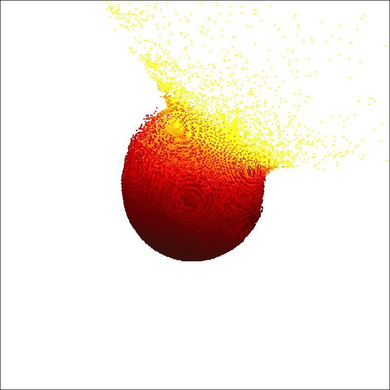
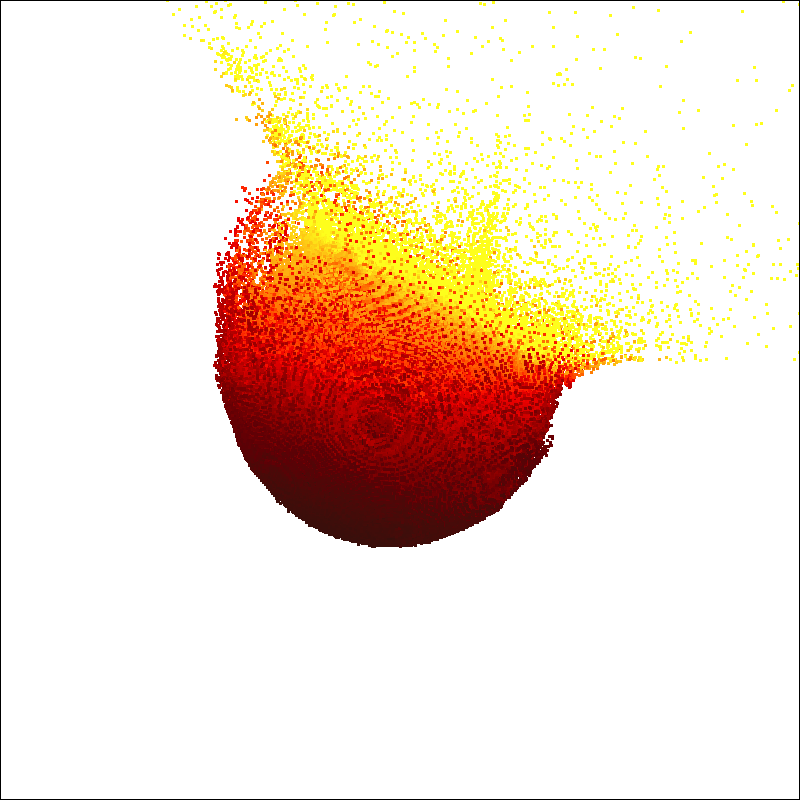
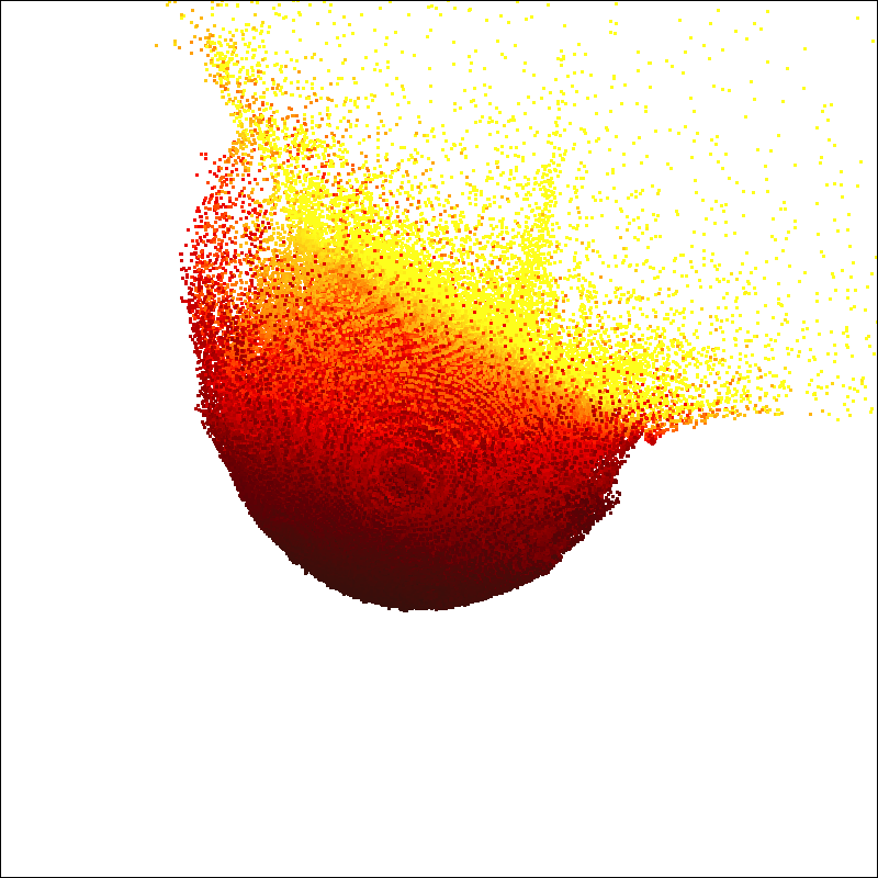
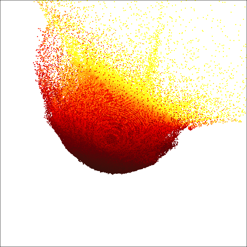
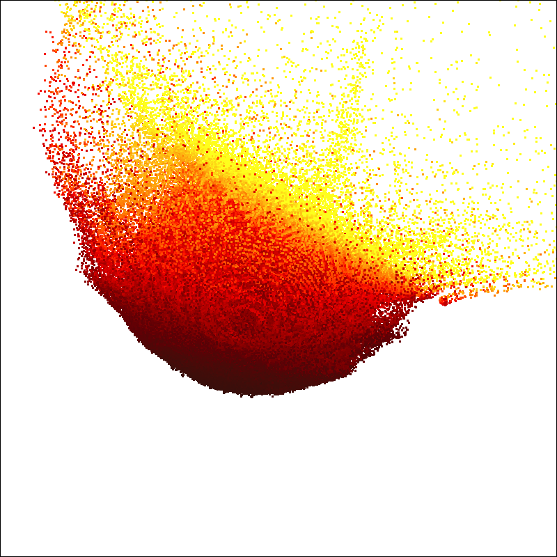
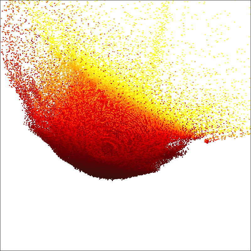
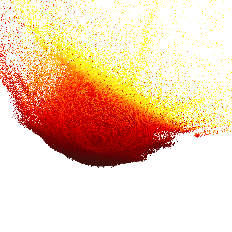
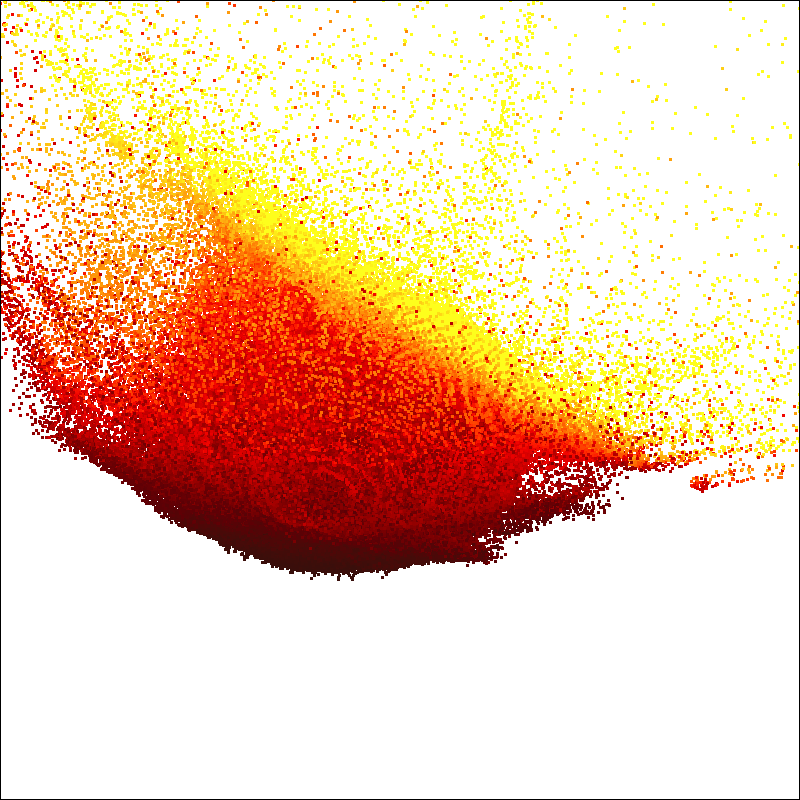
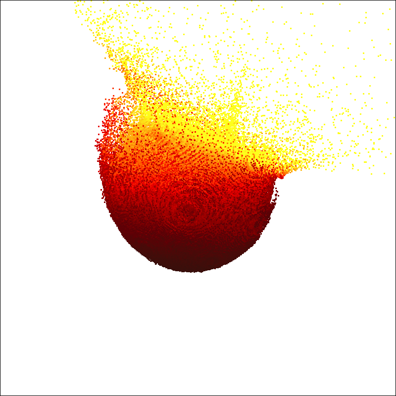
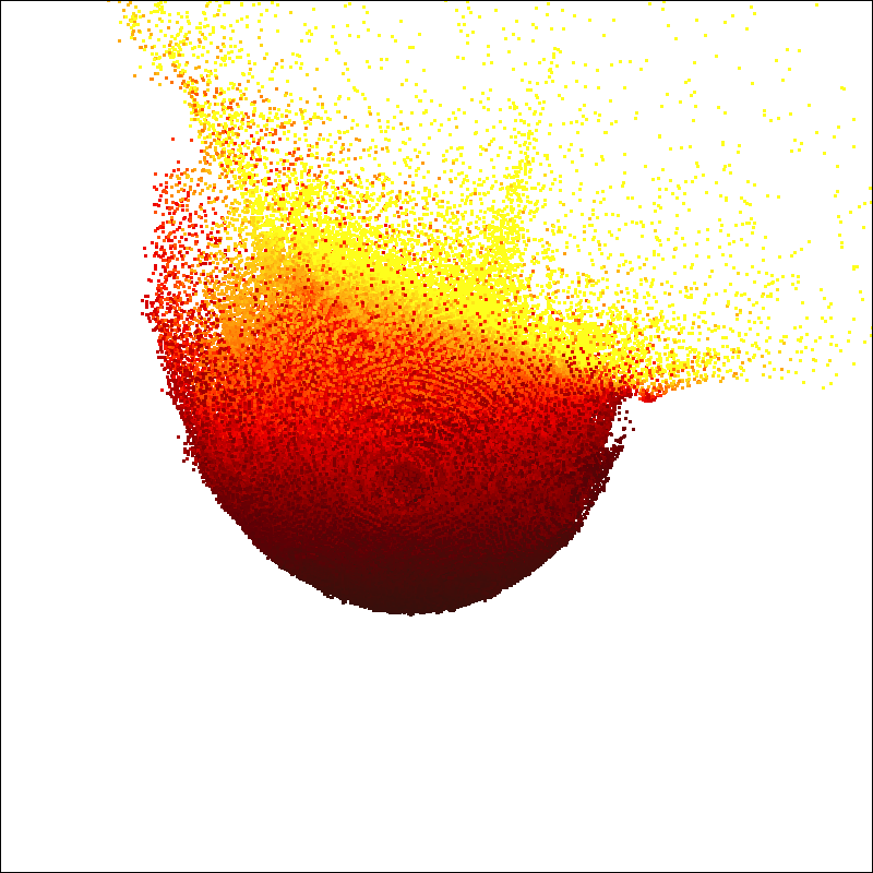
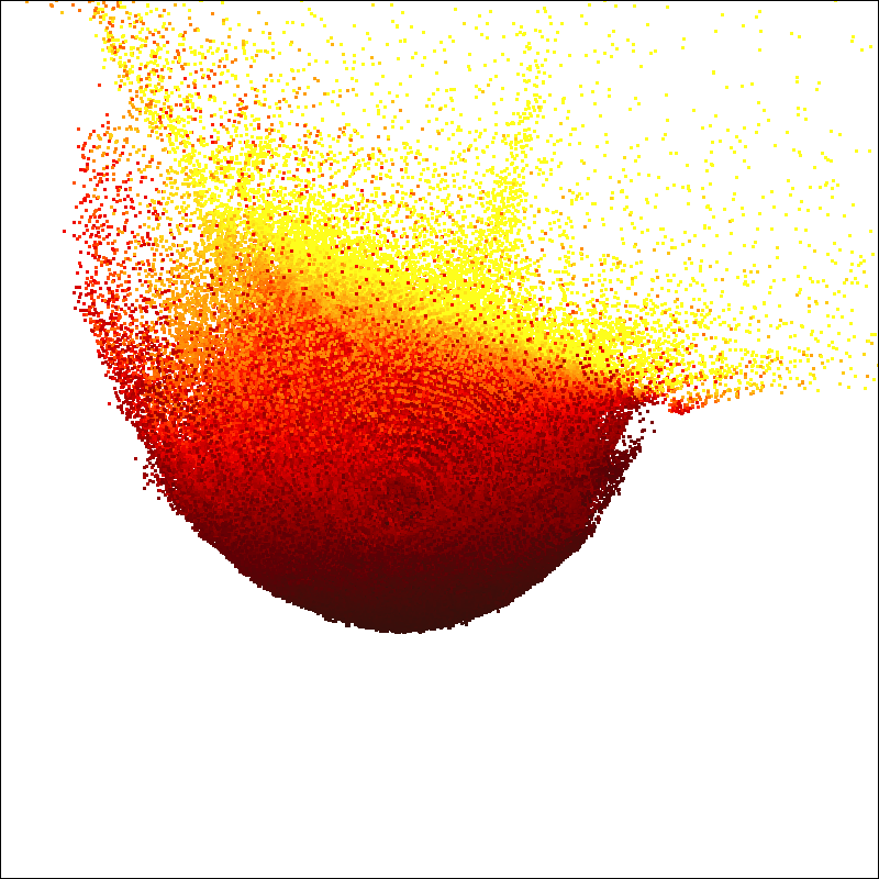
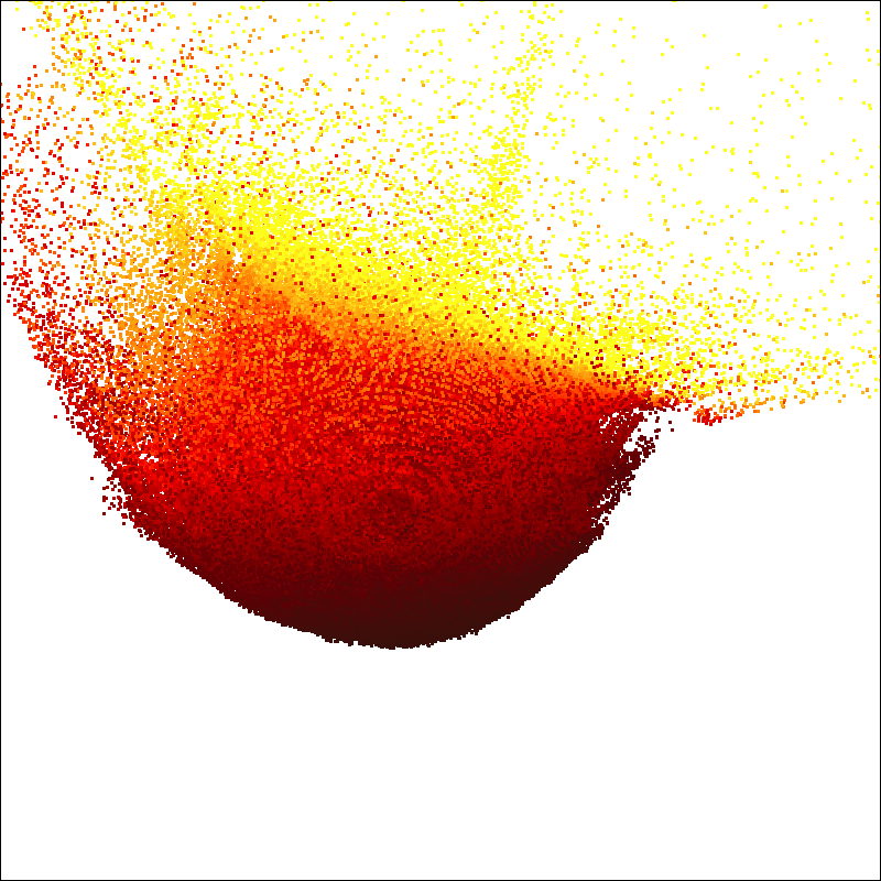
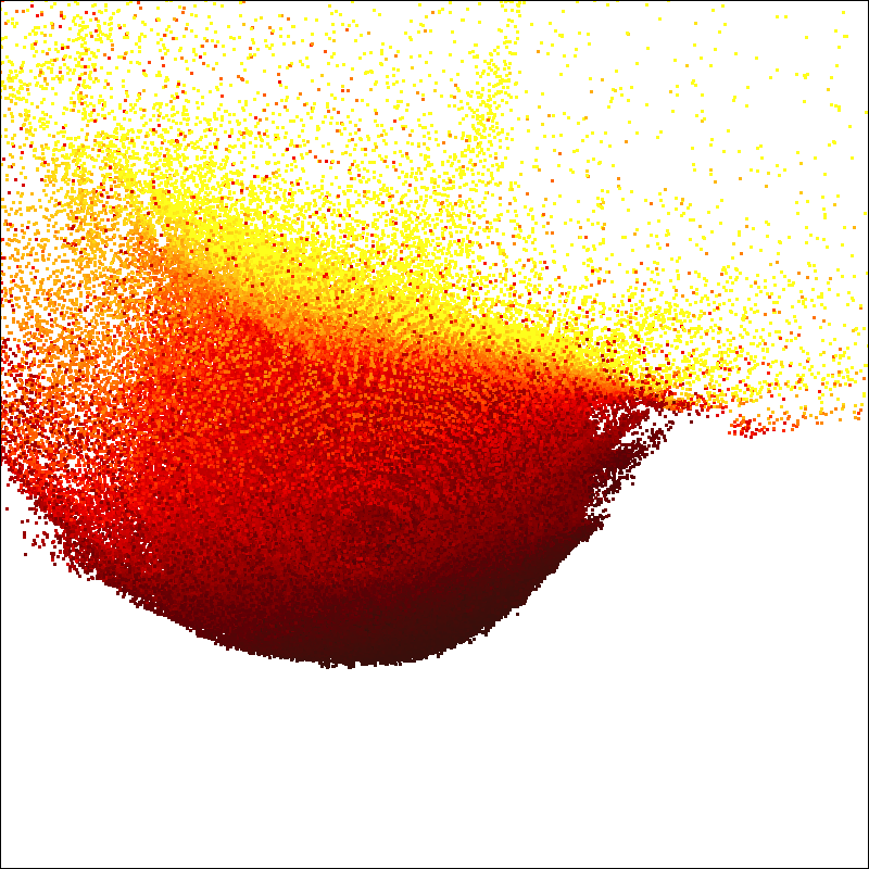
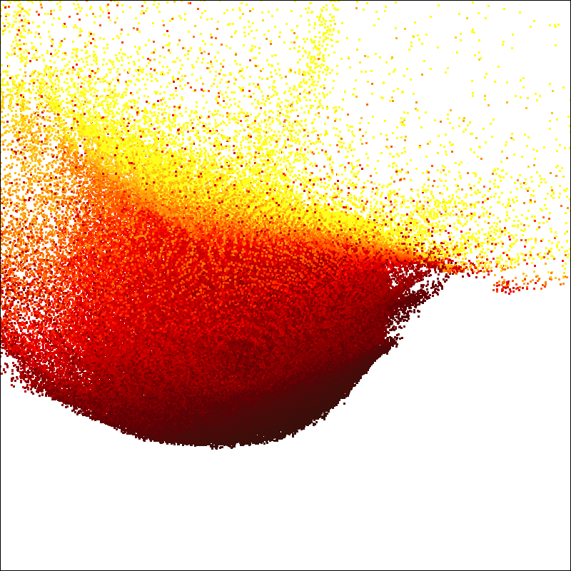
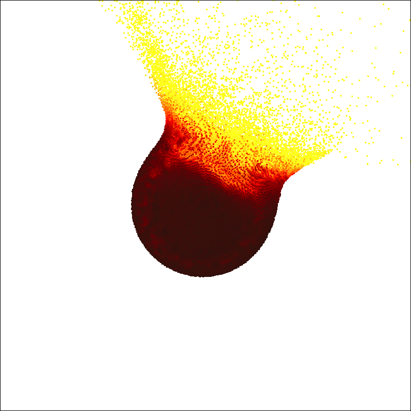
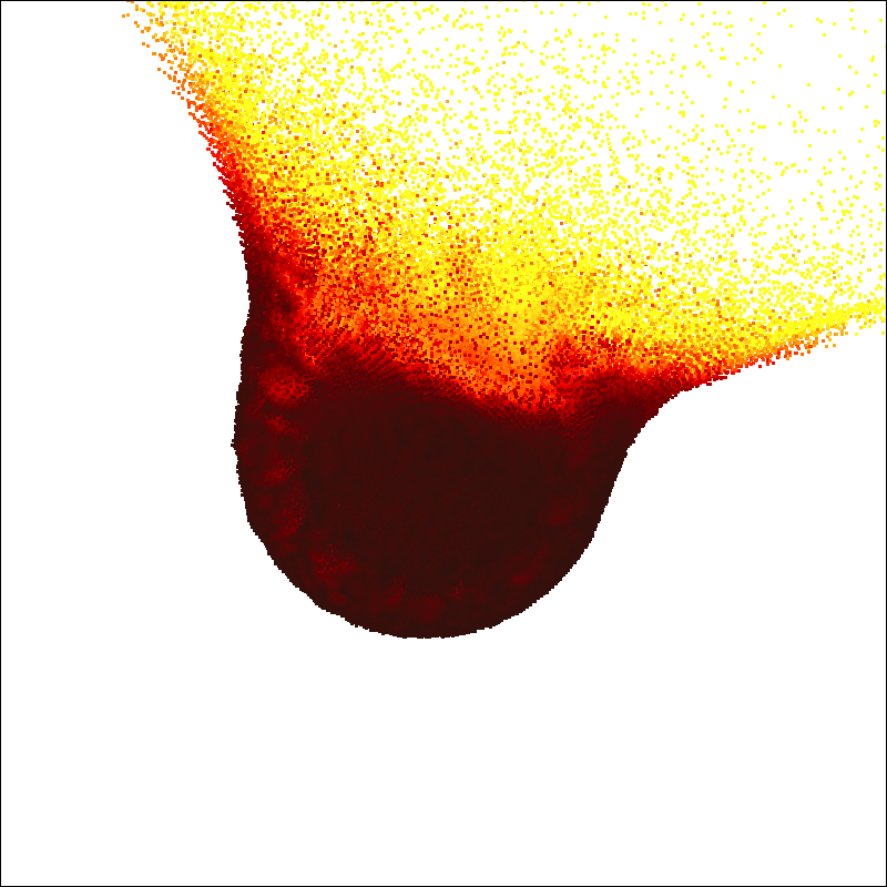
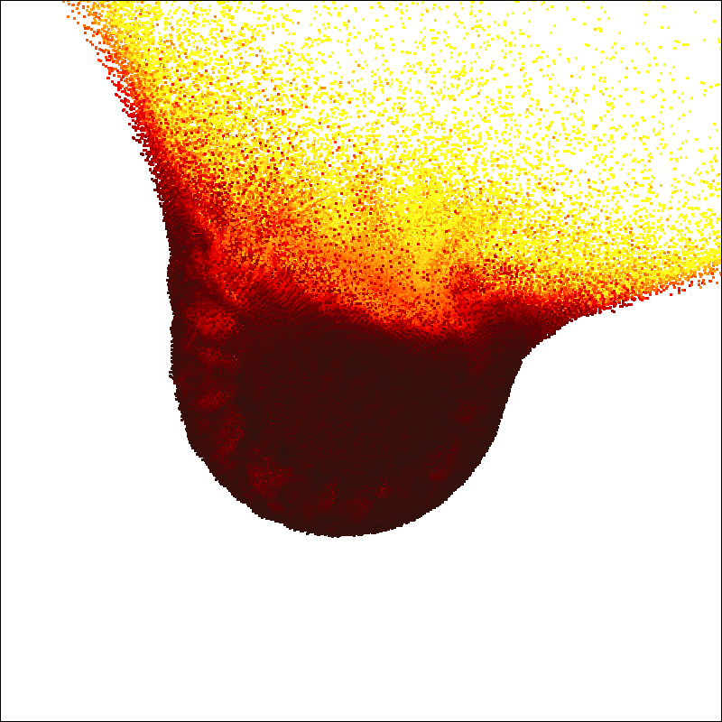
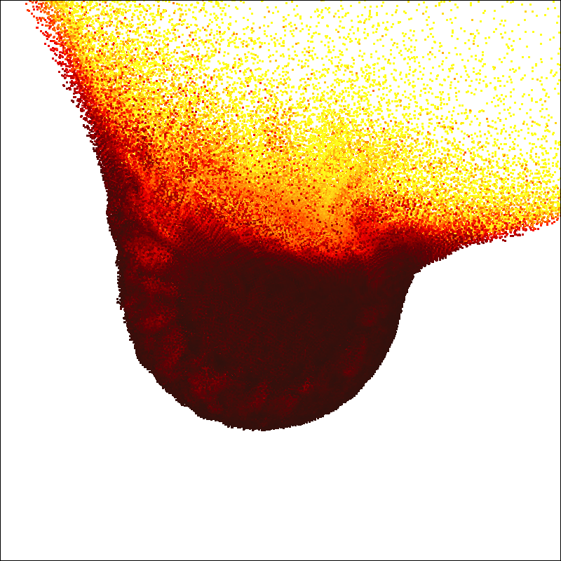
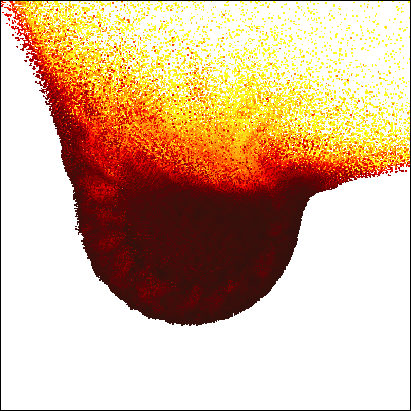
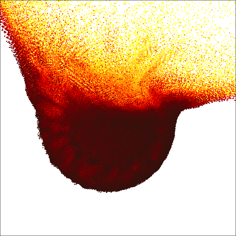
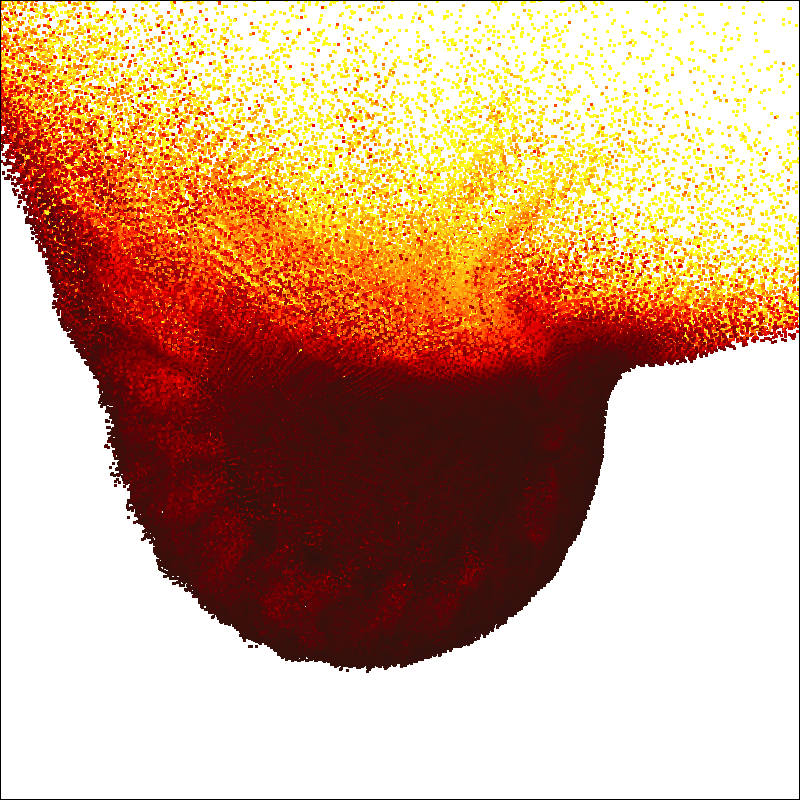
0 min 3 min 6 min 9 min 12 min 15 min 18 min 21 min 24 min

Figure 1: Impacts into $D_{\rm pb}=100\,\rm km$ targets without rotation (first row), rotational period $P_{\rm pb}=3\,\rm h$ (second row) and $P_{\rm pb}=2\,\rm h$ (third row). The period of two hours is approximately the critical period of the target. The color brightness corresponds to specific internal energy of the particles.

To better understand how the rotation influences impact events, we decided to compute a matrix of simulations for various impact parameters. We ran simulations for two different target sizes, $D_{\rm pb}=10\,\rm km$ and $D_{\rm pb}=100\,\rm km$, in order to ascertain the scaling of the rotational effect. We tested head-on impacts, having the impact angle $\phi_{\rm imp}=15^{\circ}$, intermediate cases with $\phi_{\rm imp}=45^{\circ}$ and oblique impacts with $\phi_{\rm imp}=75^{\circ}$. We have to further distinguish prograde events, i.e. impacts where the orbital velocity has the same direction as the impact velocity, and retrograde events, where the orbital velocity has the opposite direction. In the following, the prograde impacts have positive values of impact angles, while the retrograde impacts have negative.

In all of our simulations, we set the impact velocity to $v_{\rm imp}=5\,\rm km/s$, which is close to the mean velocity for Main-belt collisions (Dahlgren, 1998). The simulation matrix covers both the cratering and the catastrophic events; we ran simulations with relative impact energies $Q/{Q_{\rm D}^{\star}}=0.1,0.3,1\mbox{ and }3$, where the critical energy ${Q_{\rm D}^{\star}}$ is given by the scaling law of Benz and Asphaug (1999). As ${Q_{\rm D}^{\star}}$ is defined as the specific impact energy (relative to mass of the target) required to eject 50% of the target’s mass as fragments, it necessarily depends on the rotational period of the target. However, we consider ${Q_{\rm D}^{\star}}$ to be independent of rotation and use the same value for all performed simulations, as it provides a convenient dimensionless measure of the impact energy.

We assume that both the target and the impactor are monolithic bodies, the material parameters are summarized in Table 1. The spatial resolution of the target was approximately $N=500{,}000$ SPH particles, the number of projectile particles was selected to match the particle density of the target. Three simulations with different periods $P_{\rm pb}$ are shown in Fig. 1.

Material parameters
density at zero pressure	$\rho=2700\,\rm kg/m^{3}$
bulk modulus	$A=2.67\times 10^{10}\,\rm Pa$
non-linear Tillotson term	$B=2.67\times 10^{10}\,\rm Pa$
sublimation energy	$u_{0}=4.87\times 10^{8}\,\rm J/kg$
energy of incipient vaporization	$u_{\rm iv}=4.72\times 10^{6}\,\rm J/kg$
energy of complete vaporization	$u_{\rm cv}=1.82\times 10^{7}\,\rm J/kg$
shear modulus	$\mu=2.27\times 10^{10}\,\rm Pa$
von Mises elasticity limit	$Y_{0}=3.50\times 10^{9}\,\rm Pa$
melting energy	$u_{\rm melt}=3.4\times 10^{6}\,\rm J/kg$
Weibull coefficient	$k=4.00\times 10^{29}$
Weibull exponent	$m=9$

Table 1: Material parameters used in simulations.

3.1 Coordinate system

Due to the rotation, the impact geometry is more complex compared to the stationary case, where it was determined by a single parameter — the impact angle $\phi_{\rm imp}$ between the normal at the impact point and the velocity vector of the impactor. To describe the impact into a rotating target, we first define a coordinate system of the simulations. We place the target at origin with zero velocity, the impactor has velocity $[-v_{\rm imp};0;0]$ and its position in $x$-$y$ plane is given by $\phi_{\rm imp}$; specifically:

$$\bm{r}_{0}=\left[\begin{array}[]{l}x_{0}+0.5(D_{\rm pb}+d_{\rm imp})\cos\phi_{\rm imp},\\ 0.5(D_{\rm pb}+d_{\rm imp})\sin\phi_{\rm imp},\\ 0\end{array}\right]\,,$$

where $x_{0}$ is the distance of the impactor from the impact point. These initial conditions have a mirror symmetry in $z$.

The rotation vector $\bm{\omega}_{\rm pb}$ of the target adds additional three free parameters into the simulation setup. Generally, the vector does not have to be aligned with any coordinate axis. We reduce the number of free parameters and thus simplify the analysis by aligning the vector with $z$-axis, meaning we only consider impacts in the equatorial plane of the target. We expect these impacts will be affected by the rotation the most, as the centrifugal force is the largest on the equator. Furthermore, the angular momentum of the target is aligned with the angular momentum of the impactor, we can thus expect the largest changes of the angular momentum. These expectations have been confirmed for rubble-pile bodies by N-body simulations of Takeda and Ohtsuki (2009).

3.2 Size-frequency distributions for $D_{\rm pb}=10\,\rm km$ targets

Figure 2: Cumulative size-frequency distributions $N(>D)$ of the synthetic families for $D_{\rm pb}=10\,\rm km$ targets. Stationary targets are plotted in black, red and yellow plots correspond to targets with rotational period $P=3\,\rm h$ and $P=2\,\rm h$, respectively. Columns 3 to 5 of the plot show prograde impacts (positive impact angles), columns 1 and 2 are retrograde impacts (negative impact angles).

First set of simulations was carried out with the target size $D_{\rm pb}=10\,\rm km$. The diameters of impactors were $d_{\rm imp}=394,570,850\mbox{ and }1226\,\rm m$, respectively. We ran a number of simulations for different $P_{\rm pb}$, $d_{\rm imp}$ and $\phi_{\rm imp}$ and compared the size-frequency distribution of a family created by an impact into a rotating target with corresponding impact into a stationary target. The resulting distributions are plotted in Fig. 2.

At first glance, the differences between the targets rotating with period the $P_{\rm pb}=3\,\rm h$ and the non-rotating targets are relatively small. The slope of the SFD is almost unchanged in most simulations, it is only shifted as more mass is ejected from the rotating target. In several simulations, e.g. for $\phi_{\rm imp}=-45^{\circ}$ and $d_{\rm imp}=0.85\,\rm km$, we can see a larger number of fragments in the middle part of the SFD for rotating targets; fragments that would reaccumulate to the largest remnant in the stationary case now escape due to the extra speed from rotation and contribute to the family.

Much larger differences in SFDs can be seen for the target with period $P_{\rm pb}=2\,\rm h$, which is rather expected; for $\rho_{0}=2700\,\rm kg/m^{3}$ the critical period is $P_{\rm crit}\simeq 2.009\,\rm h$, so a $P_{\rm pb}=2\,\rm h$ target actually rotates very slightly supercritically, although is is held stable by the material strength. The difference is the most prominent for oblique $\phi_{\rm imp}=\pm 75^{\circ}$ impacts. In several cases, the rotation seems to make the SFD less steep, although this might be partially attributed to a numerical artifact, as the synthetic families of non-rotating targets are already very close to the resolution limit.

On the other hand, energetic impacts produce practically the same SFDs regardless of $P_{\rm pb}$. In this regime, angular momentum of projectiles is larger than the rotational angular momentum of the target; for $Q/{Q_{\rm D}^{\star}}=3$ and $P_{\rm pb}=2\,\rm h$, the angular momentum of a projectile is larger 5x. Ejection velocities are also considerably larger than orbital velocities, hence it is not surprising that the rotation does not make a substantial difference.

It is not probable that these differences come from different fragmentation pattern, as targets are fully damaged by the impact. In our model, such damaged material is strengthless and it essentially behaves like a fluid. Since there is no internal friction or a mechanism to regain the material strength, this model is insufficient to determine shapes of the fragments; however, here we are only interested in size distributions and using a simplified model is therefore justified.

3.3 Size-frequency distributions for $D_{\rm pb}=100\,\rm km$ targets

Figure 3: Cumulative size-frequency distribution for $D_{\rm pb}=100\,\rm km$ targets. The notation is the same as in Fig. 2.

It is a priori not clear how rotation affects targets of different sizes. To preliminary estimate the importance of initial rotation, we compute the ratio of the angular frequency $\omega_{\rm pb}$ of the target and $\omega_{\rm imp}$ of the impactor with respect to the target:

$$\frac{\omega_{\rm pb}}{\omega_{\rm imp}}\sim\frac{D_{\rm pb}}{v_{\rm imp}P_{\rm pb}\sin\phi_{\rm imp}}\,.$$ (21)

Because the ratio scales linearly with the target size $D_{\rm pb}$, we expect that the rotation will play a bigger role for impacts into larger targets; however, this back-of-the-envelope computation is by no means a definite proof and it needs to be tested.

To this point, we ran a set of simulations with target size $D_{\rm pb}=100\,\rm km$. The set is analogous to the one in Sec. 3.2 — we use the same impact angles and rotational periods, the impactor diameters were $d_{\rm imp}=11.170,16.110,24.064\mbox{ and }34.706\,\rm km$ in order to obtain the required relative energies $Q/{Q_{\rm D}^{\star}}$. The size-frequency distributions of the synthetic families are plotted in Fig. 3.

As expected, the differences between rotating and non-rotating targets are indeed substantially larger than for $D_{\rm pb}=10\,\rm km$. The rotation can completely change the impact regime from cratering to catastrophic; see e.g. the impact with $\phi_{\rm imp}=15^{\circ}$ and $d_{\rm imp}=16.110\,\rm km$, where a cratering gradually changes to a catastrophic disruption as we decrease $P_{\rm pb}$. Focussing on $P_{\rm pb}=3\,\rm h$ targets, they produce very shallow SFD in case of oblique prograde impacts. For $\phi_{\rm imp}=\pm 45^{\circ}$ cratering impacts, we see numerous intermediate-sized fragments (somewhat separated in the SFD) if the target is non-rotating, but the SFD becomes continuous when rotation is introduced.

The effects are even stronger for critically rotating bodies with $P_{\rm pb}=2\,\rm h$, of course. Generally, SFDs of formally cratering events are more similar to catastrophic ones. It also seems that oblique retrograde craterings produce more fragments than prograde ones. For the impact $\phi_{\rm imp}=15^{\circ}$ and $d_{\rm imp}=24.064\,\rm km$, the SFD is well below the non-rotating case and most of the mass is contained in smallest fragments.

Although large ($D\gg 10\,\rm km$) asteroids typically rotate much slower than smaller bodies, there are few that rotate close to the critical spin rate for elongated bodies, such as (216) Kleopatra (Hirabayashi and Scheeres, 2014). Rotation in collisional simulations of such bodies should therefore not be neglected.

3.4 Total ejected mass

Figure 4: The total mass of fragments $M_{\rm ej}(P)/M_{\rm ej}(\infty)$ ejected by collisions, normalized by the mass of fragments from a corresponding collision into a stationary target. Four figures correspond to different relative impact energies, from cratering (left) to mid-energy (right) events. The ejected mass is plotted as a function of the impact angle $\phi_{\rm imp}$ and initial period $P_{\rm pb}$ of the target.

While Figs. 2 and 3 clearly show the differences between the SFDs, it is quite difficult to read the total mass ejected from the target during the impact. Even when the SFDs of a rotating and a stationary target seem to differ only negligibly, the total integrated mass of fragments may be significantly different.

To show the effect of the initial rotation on the ejected mass clearly, we performed over 400 simulations with the target size $D_{\rm pb}=10\,\rm km$ and various impact angles $\phi_{\rm imp}$, projectile diameters $d_{\rm imp}$ and initial periods $P_{\rm pb}$ of the target. These simulations have a lower spatial resolution compared to the simulations of family formation in previous sections, as here we need not to resolve individual fragments in detail. The target is resolved by approximately $N=100000$ particles.

We ran simulations for $\phi_{\rm imp}$ ranging from $15^{\circ}$ to $75^{\circ}$ (both prograde and retrograde). To capture the dependence on $P_{\rm pb}$, we selected nine different values from $P_{\rm pb}=P_{\rm crit}$ to $50P_{\rm crit}$. The impact energies of the simulations were $Q/{Q_{\rm D}^{\star}}=0.03,0.1,\,0.3\mbox{ and }1$, meaning the simulations range from cratering events to mid-energy events.

Our goal is to compute the total mass of the fragments as a function of the impact angle $\phi_{\rm imp}$, the initial rotational period $P_{\rm pb}$ and the diameter $d_{\rm imp}$. We are actually not interested in the absolute value of the ejected mass, but rather in the ejected mass relative to the mass that would be ejected if the targets were stationary. Therefore, we compute the ratio:

$$\mu_{\rm ej}=\frac{M_{\rm ej}(\phi_{\rm imp},d_{\rm imp},P_{\rm pb})}{M_{\rm ej}(\phi_{\rm imp},d_{\rm imp},\infty)}$$ (22)

and plot the result in Fig. 4. Values $\mu_{\rm ej}<1$ would mean that the impact into the rotating target ejected fewer fragments, compared to the stationary target; no such result was found in the performed simulations.

Generally, the rotation amplifies the ejection by several tens of percent. However, the increase is significantly higher if the following conditions are satisfied:

• Target rotates near the critical period. The effect of rotation decreases rapidly with increasing period of the target, as expected.

• The impact results in a cratering rather than a catastrophic event. While high-energy impacts eject more fragments in an absolute measure, the initial rotation does not affect the value notably in this regime.

• The impact is oblique and has a prograde direction. Head-on impacts and the impacts in retrograde directions are not affected by the rotation to the same degree.

In extreme cases, the rotation can amplify the ejected mass by a factor of 5. On the other hand, the ejection ratio $\mu_{\rm ej}$ does not exceed 1.6 for rotational periods $P_{\rm pb}>2P_{\rm crit}$ in any of the performed simulations.

Although it is a different rheology, rubble-pile bodies also exhibit a minor effect of rotation (on $Q^{\star}_{\rm D}$ as well as $\mu_{\rm ej}$) in this range of $P_{\rm pb}$ (Takeda and Ohtsuki, 2009, see Fig. 2 therein). However, their strength is an order of magnitude lower than for monoliths of Benz and Asphaug (1999), so the comparison is not straightforward.

4 Embedding and draining the angular momentum

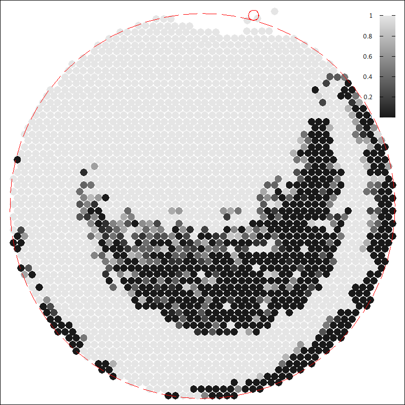
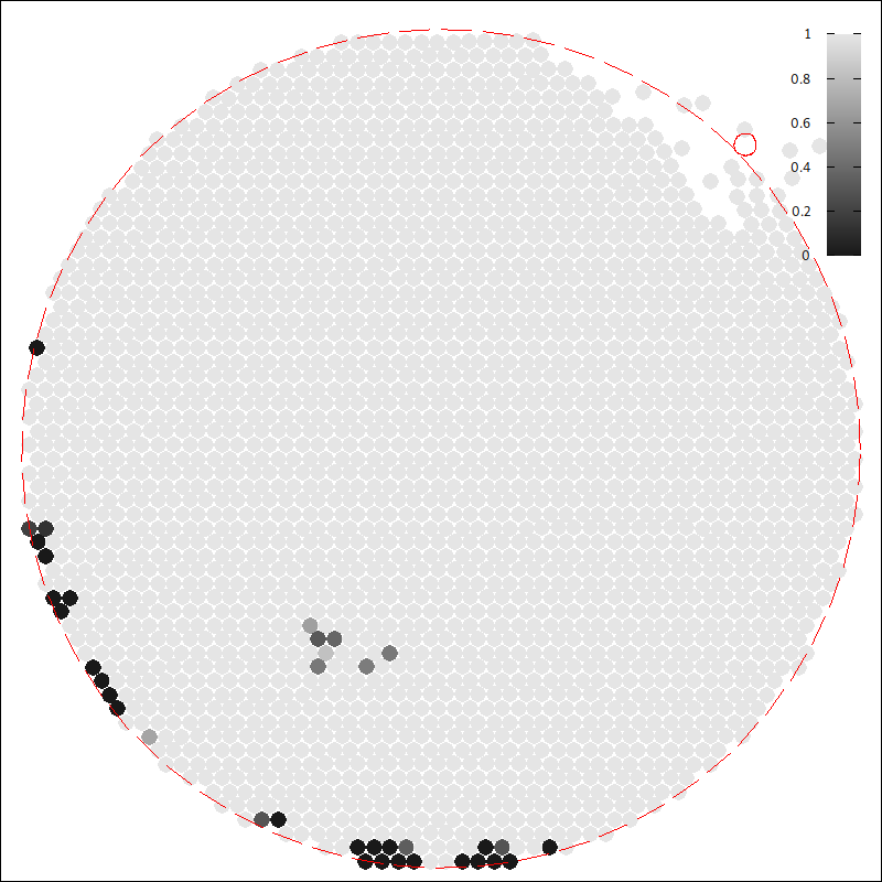
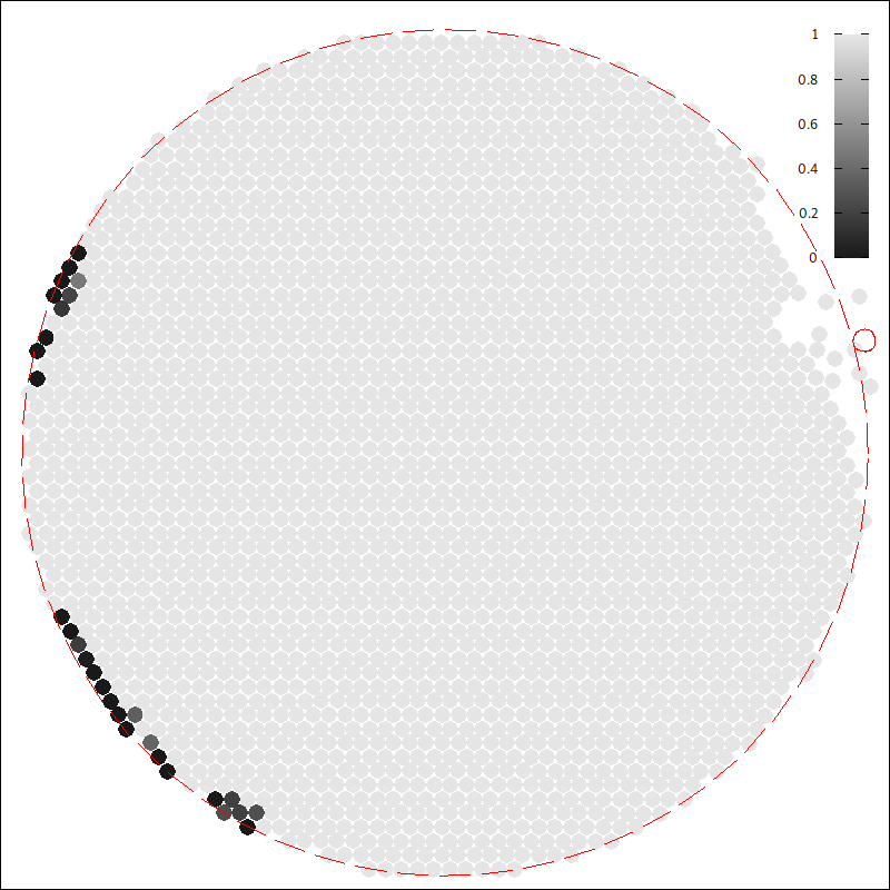
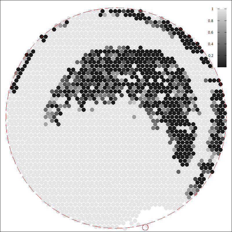
Figure 5: Damage of the target at time $t=10\,\rm s$ after the impact for various impact angles; from left to right, $\phi_{\rm imp}=75^{\circ},45^{\circ},15^{\circ},-45^{\circ},-75^{\circ}$. Simulations were carried out with the impactor of size $d_{\rm imp}=314\,\rm m$ and speed $v_{\rm imp}=5\,\rm km/s$, target was not rotating. Red outline shows the original position of the target and the impactor. There is an undamaged cavity only for oblique impacts, otherwise the target is fully damaged by the impact.

Figure 6: Change of the spin rate $\Delta\omega$ of the target (or the largest remnant in case $Q/{Q_{\rm D}^{\star}}\simeq 1$) as a function of the initial period $P_{\rm pb}$ of the target (here in units of the critical period $P_{\rm crit}$) and the impact angle $\phi_{\rm imp}$. Four images correspond to different sizes of the impactor, the energy of the impact is from left to right $Q/{Q_{\rm D}^{\star}}=0.03,0.1,0.3\hbox{ and }1$. The impact velocity was $v_{\rm imp}=5\,\rm km/s$ in all cases.

Figure 7: Dimensionless effectivity $\gamma$ of the angular momentum transfer. Other quantities are the same as in Fig. 6.

Impact into a rotating target can cause either an acceleration or a deceleration of the target’s rotation. This can be immediately seen from two limit cases: a stationary target is always spun by the impact, on the other hand a target rotating at the breakup limit cannot be accelerated any further and the collision thus always causes a deceleration.

It has been proposed that rotating asteroids are decelerated over time by numerous subsequent cratering collisions, as a fraction of the angular momentum is carried away by fragments. Coined the angular momentum drain (Dobrovolskis and Burns, 1984), this effect could explain the excess of slow rotators in the Main Belt. In this section, we examine whether this effect emerges in our simulations and we determine the functional dependence of the deceleration on the impact parameters.

We analyze the angular momentum transfer as a function of impact parameters, using the set of simulations described in Sec. 3.4. The impacts range from cratering ($Q/{Q_{\rm D}^{\star}}\sim 0.03$) to mid-energy ($Q/{Q_{\rm D}^{\star}}\sim 1$) events. For $Q/{Q_{\rm D}^{\star}}\sim 1$, the whole target asteroid is disintegrated by the collision and fragments with mass of about $0.5M_{\rm pb}$ are reaccumulated later, forming the largest remnant. This can no longer be viewed as a cratering event that merely modifies the rotational state of the target, nevertheless we can still formally compute the relation between the period of the target and the largest remnant.

In majority of performed simulations, the target is completely damaged by the impact. Only for the weakest oblique impacts with $Q/{Q_{\rm D}^{\star}}=0.03$, there remained an undamaged cavity, as shown in Fig. 5, otherwise all particles of the target have damage $D=1$ after the fragmentation phase.

The change of spin rate $\Delta\omega$ of the target is plotted in Fig. 6. We plot the change of frequency rather than period, as the period is formally infinite for a non-rotating body; change of period is thus not a meaningful quantity.

For cratering events, the prograde events (denoted with positive $\phi_{\rm imp}$) mostly accelerate the target, while retrograde events cause deceleration. The two exceptions from this rule are:

1. a prograde impact into a critically rotating body, in which case it cannot be accelerated any more and some deceleration is expected,

2. a retrograde impact to an almost stationary body.

Impacts with higher energies show a different pattern. It seems that the two regions described above expand. Prograde impacts into fast rotators actually decelerate the target, while retrograde impacts start to accelerate it. For the most energetic event we studied, $Q/{Q_{\rm D}^{\star}}\simeq 1$, it seems that the two regions completely swapped — most prograde impacts cause a deceleration while retrograde ones an acceleration.

The despinning (or angular momentum draining) on rubble-piles in catastrophic disruptions was confirmed by Takeda and Ohtsuki (2009). In our simulations, the pattern is more complex, likely because the parameter space ($Q/Q^{\star}_{\rm D}$, $P_{\rm pb}$) is significantly more extended; also rubble-piles cannot initially rotate critically.

4.1 Effectivity of the angular momentum transfer

Let us define the effectivity $\gamma$ of the angular momentum transfer as:

$$\gamma\equiv\frac{L_{\rm lr}-L_{\rm pb}}{L_{\rm imp}}\,,$$ (23)

where $L_{\rm pb}$ is the rotational angular momentum of the target before the impact, $L_{\rm pb}$ is the rotational angular momentum of the largest remnant and $L_{\rm imp}$ is the angular momentum of the impactor with respect to the target. As these values are scalars, we assign a negative sign to the value $L_{\rm imp}$ for retrograde impacts.

We emphasise that the effectivity $\gamma$ is not necessarily in the unit interval $\langle 0;1\rangle$. Specifically, it may be significantly larger than 1 for head-on impacts, as the delivered angular momentum is very low; in fact, $L_{\rm imp}$ approaches zero for $\phi_{\rm imp}=0$. The effectivity can also be a negative number for impacts to critically rotating targets, as in these cases, the target cannot accelerate over the breakup limit, so a zero or even negative values of $\gamma$ are expected.

The effectivity $\gamma$ as a function of the initial period $P_{\rm pb}$, the impact angle $\phi_{\rm imp}$ and the impactor diameter $d_{\rm imp}$ is plotted in Fig. 7. We can see that cratering impacts have generally higher effectivity than high-energy impacts. This result might have been expected, as the cratering impacts eject less mass and thus transfer less angular momentum to fragments, compared to the catastrophic impacts. A less expected outcome is the negative effectivity for the high-energy impacts. We predicted the negative values only for prograde impacts into critically rotating targets, but for $d_{\rm imp}=850\,\rm m$ the effectivity is negative for the majority of performed simulations.

Finally, the highest effectivity is achieved for retrograde impacts into critically rotating targets. However, this results is a bit fake, because in this regime the target is always decelerated, $\gamma$ can therefore exceed 1 as the angular momentum lost in the collision is higher than $L_{\rm imp}$ (in absolute value). Impacts into slower rotators have values of $\gamma$ around 0.5.

4.2 Angle-averaged ejection and momentum transfer

To express an overall effect of collisions on a rotational state of a target, it is useful to consider a large number of collisions at random impact angles and compute the average change of spin rate:

$$\overline{\Delta\omega}\equiv\int\limits_{0}^{\pi/2}\Delta\omega\sin 2\phi\,{\rm d}\phi\approx\frac{\sum_{i}\Delta\omega_{i}\sin 2\phi_{i}}{\sum_{i}\sin 2\phi_{i}}\,,$$ (24)

where $\sin 2\phi$ is the probability of the impact with the impact angle $\phi$. The averaged change $\overline{\Delta}\omega$ is plotted in Fig. 8, together with a plot of the relative mass ejection $\overline{\mu}_{\rm ej}$, defined in Sec. 3.4.

The figures show that targets are on average decelerated for both low-energy and mid-energy impacts. A target is only accelerated if it was originally a very slow rotator, since it cannot be decelerated any more. The transition between these two regimes (plotted in white) is where the target does not change its angular frequency upon the impact. It seems to depend on the energy of the impact; for $Q/{Q_{\rm D}^{\star}}\sim 0.1$, the transition occurs at around $P\sim 20P_{\rm crit}$, while for $Q/{Q_{\rm D}^{\star}}\sim 1$, it is shifted to around $P\sim 6P_{\rm crit}$.

Figure 8: Quantities averaged over impact angles using Eq. (24) as a function of period $P_{\rm pb}$ of the target and the impactor diameter $d_{\rm imp}$. The left figure shows the change of spin rate $\Delta\omega$, the right one the total mass of fragments, normalized by the mass of fragments from corresponding collision into a stationary target.

5 Conclusions and future work

In this paper, we showed that a fast initial rotation of targets may significantly affect resulting synthetic families. The effect is more prominent for larger target bodies and for oblique impact angles. Generally, more fragments is ejected from prograde ($\phi_{\rm imp}>0$) compared to the retrograde ($\phi_{\rm imp}<0$) targets.

In extreme cases, the mass ejection can be amplified by a factor 5. Neglecting the rotation would therefore introduce a considerable bias. Other parameters of the simulation do introduce similar (or sometimes larger) uncertainties, for example the Weibull parameters of the fragmentation model (Ševeček et al., 2017), the rheological model of the target, etc. As shown in Jutzi and Benz (2017), the initial shape can also have a significant effect.

Throughout this paper, we assumed that both the targets and impactors are monolithic bodies. It is a priori not clear whether the rotation would be more important for rubble-pile bodies (with macro-porosity), or when a rheological model with crushing (micro-porosity) is used in the simulations (Jutzi et al., 2019). It should also be explored how initial shapes relate to spin rates of fragments. We postpone such studies to future works.

In the future, we also plan to determine the scaling law as a function of both $D_{\rm pb}$ and $P_{\rm pb}$. It is clear that the critical energy ${Q_{\rm D}^{\star}}$ is a steep function of $P_{\rm pb}$ close to the critical spin rate. Finding a functional dependence ${Q_{\rm D}^{\star}}={Q_{\rm D}^{\star}}(P_{\rm pb})$ might be a valuable result for studies of Main Belt evolution, as it could be used to construct a combined model that includes both collisions and rotations.

Appendix A Handling particle overlaps

Since we treat particles as solid spheres during the reaccumulation phase, particle overlaps are unavoidable and need to be handled by our N-body integrator. There are two main reasons why particle overlaps occur.

First, the spheres overlap initially after the hand-off (Eq. 18). In SPH, the particles naturally overlap as they describe a continuum rather than point masses. After converting them to solid spheres, particles belonging to the same body will necessarily overlap, unless their radius is decreased significantly.

Second, overlaps occur when particles are being merged. When two spherical particles collide, they merge into a larger particle with volume equal to the sum of volumes of the colliders. This merging is an atomic operation, particles are converted into the merger in an instant rather than over several timesteps, so any other particles located close to the colliders potentially overlap the particle merger.

Our code allows for several options to resolve overlaps. One straightforward solution is to always merge the overlapping particles. While this is a simple and robust solution, it can potentially create unphysical, supercritically rotating bodies. Alternatively, we can repel the overlapping particles, so that they are in contact rather than overlap. However, this causes an “inflation” of the largest remnant after the hand-off. Even worse, the angular momentum is no longer conserved.

Another option is to abandon the 1-1 conversion of spheres and instead construct a new set of spheres inside the alpha-shape of the largest remnant (Ballouz et al., 2018). Such approach allows to place spheres onto a regular grid and thus avoid overlaps by construction. However, it is more suitable when collided particles form rigid aggregates instead of mergers. As spheres never fill the entire volume (filling factor of hexagonal close packing is about 0.74) and the merging conserves volume, fragments would shrink considerably.

We decided to merge particles only if the spin rate of the would-be merger is lower than the critical spin rate, otherwise we allow particles to pass through each other. Of course, such handling is only applied to resolve overlaps, particles that collide are always treated as solid.

Appendix B Comparison of inertial and co-rotating reference frames

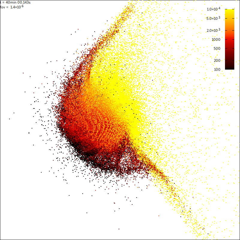
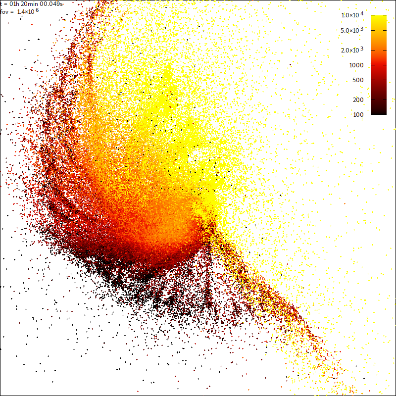
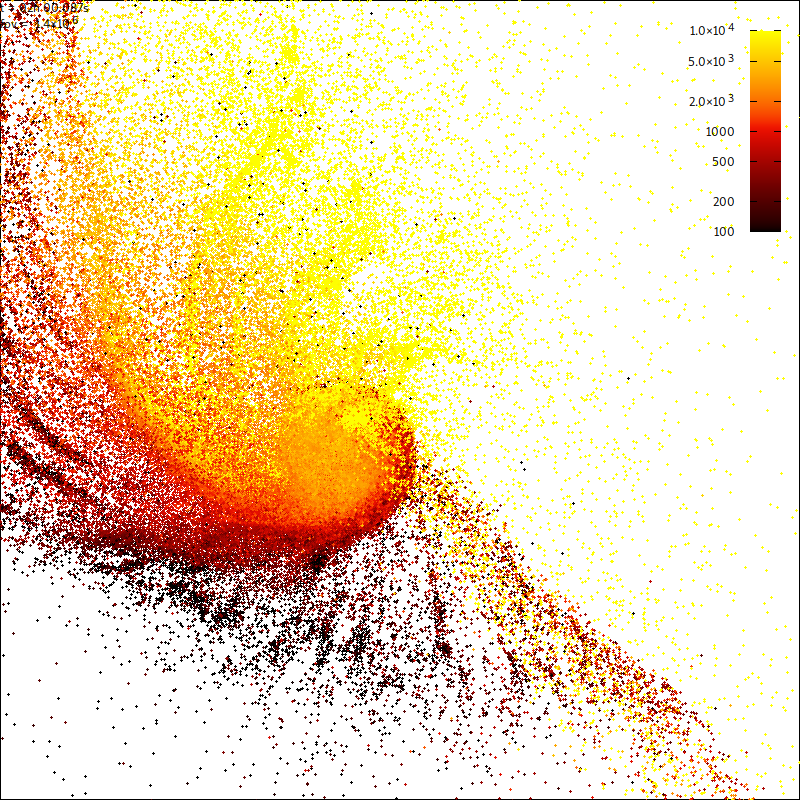
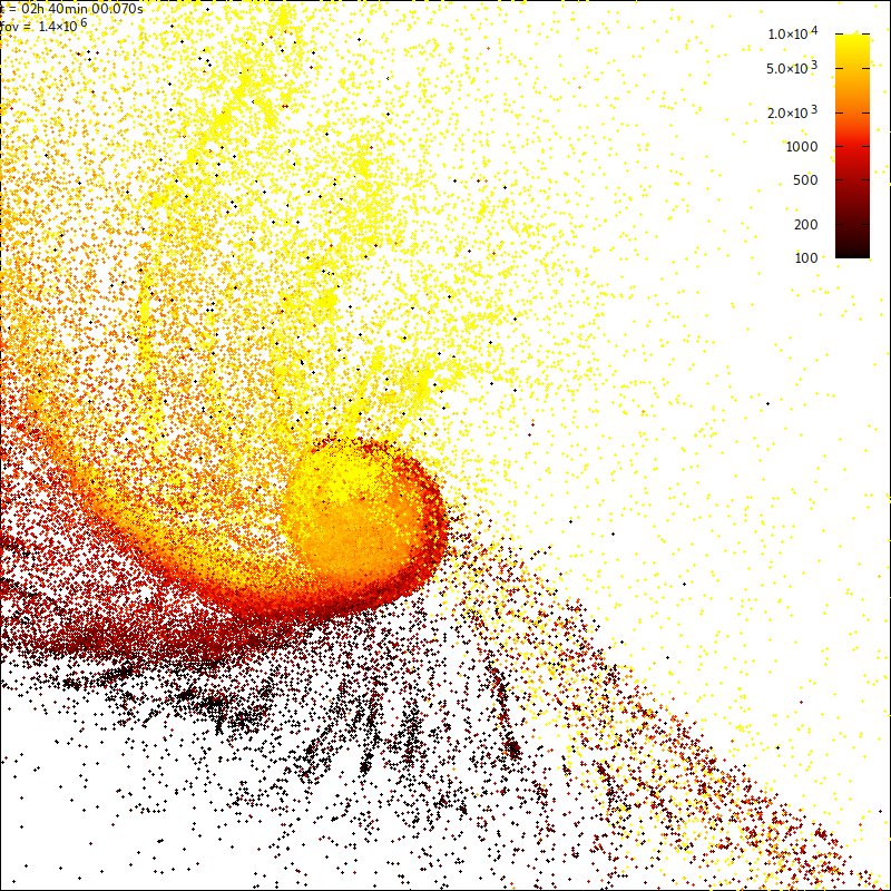
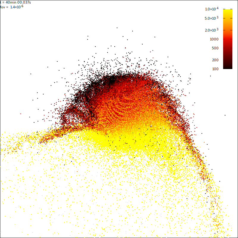
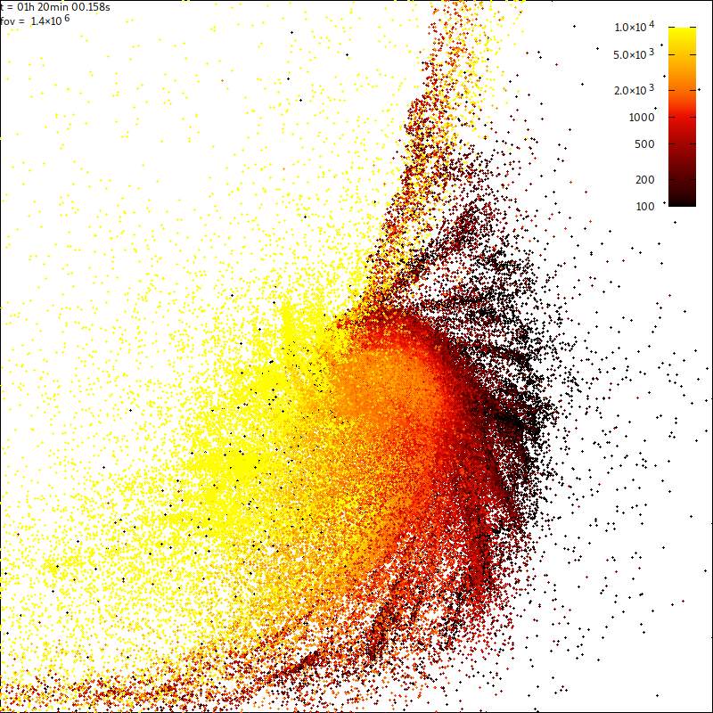
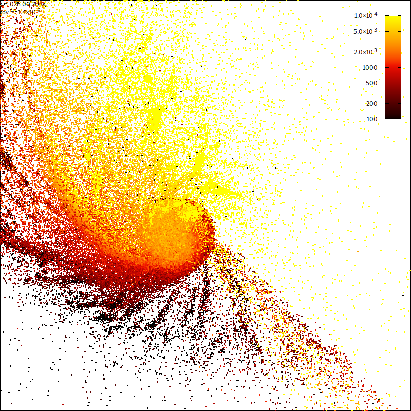
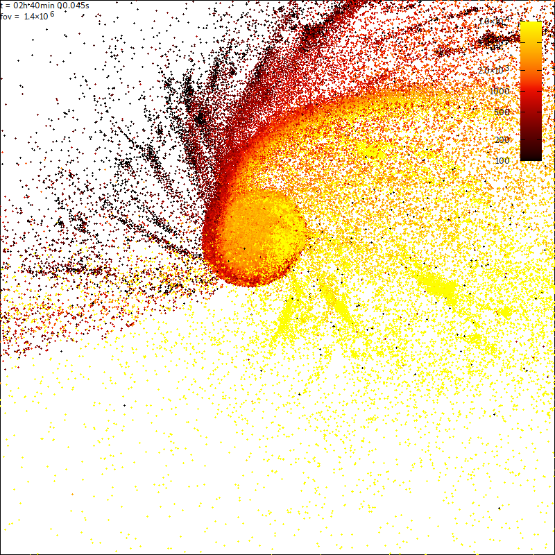
Figure 9: Impact into $D_{\rm pb}=200\,\rm km$ target, computed with rotating target (upper row) and with rotating coordinate frame in which the target is stationary (lower row), plotted at times $t=40,80,120\mbox{ and }160\,\rm min$ after the impact. The color scale represents the specific energy of the particles (in SI units).

We can choose two different approaches to implementing the rotation of the target:

1. rotate the particles around the center of the target,

2. perform the simulation in the coordinate system co-rotating with the target.

From a numerical point of view, the second approach is easier to handle, as the particles of the target have initially zero velocities and we thus avoid numerical problems with the bulk rotation outlined in Sec. 2.1. The rotation is taken into account by introducing inertial accelerations, i.e. the last two terms of Eq. (2).

However, it only solves the issue partially; even though the target is stationary (in the co-rotating frame) before the impact, the projectile can spin up the target and the impact can also eject rotating fragments. To properly handle rotating bodies in SPH, it is necessary to introduce the correction tensor Eq. (5). This allows us to perform simulations in the inertial frame, which is a natural choice.

Ideally, these two approaches should produce identical results. To test it, we ran two simulations with $D_{\rm pb}=200\,\rm km$ parent bodies rotating critically. The results are plotted in Fig. 9. We observe some stochastic differences, but the spatial distribution of the ejected fragments is similar in both simulations. This test confirms the consistency of both approaches.

Appendix C Implementation notes

The code OpenSPH used throughout this work is open-source, available under MIT license. As of , it can be be downloaded from https://gitlab.com/sevecekp/sph. It includes a helpful graphical interface, allowing to interactively visualize the simulation, see Fig. 10. It is also a standalone viewer of OpenSPH output files and potentially files generated by other particle-based codes, provided their file formats are implemented.

Our code can be used as both an SPH solver and an N-body integrator, as we separated computation of SPH derivatives and gravitational accelerations. In each time step, accelerations due to hydrodynamics and gravity are computed independently and summed up. Even though we miss some optimization possibilities with this approach, it allows us to use the same code for both the fragmentation and the reaccumulation phase; the hand-off is thus only an internal change of a solver, replacing SPH hydrodynamics with a collision detection.

We use the Barnes-Hut algorithm to evaluate gravitational accelerations (Barnes and Hut, 1986). The code uses the same functionality in SPH and N-body solver, it only differs in the softening kernel $\phi$; in SPH, it is defined by Eq. 14, while for N-body it corresponds to a homogeneous sphere. Our implementation uses a k-d tree, which is also used to find particle neighbours.

In the fragmentation phase, we found that the time step criterion which uses stress tensor derivatives (Eq. 16) is often unnecessarily restricting, as the stress tensor changes rapidly inside the projectile. However, we are not very interested in remnants of projectiles, simulations can be thus sped up by applying the criterion only for particles of the target. No such optimization is applied for CFL criterion, as it determines stability of the method and it is thus essential for all particles.

In the reaccumulation phase, collided particles are merged, provided their relative velocity does not exceed the escape velocity $v_{\rm esc}$ (as in Eq. 19) and the spin rate does not exceed the critical spin rate $\omega_{\rm crit}$ (as in Eq. 20). In practice, both $v_{\rm esc}$ and $\omega_{\rm crit}$ are multiplied by user-defined factors (i.e. a merging limit). It may be useful to tune it in such a way that a simplified N-body model of reaccumulation matches a full SPH simulation (in terms of resulting SFDs).

The total CPU time needed depends on a type of simulation. Generally, catastrophic impacts take longer to compute than cratering impacts (quantities change more rapidly, hence smaller time steps are needed), smaller targets usually mean longer computation time (smaller SPH particles, which implies smaller time steps due to the Courant criterion). The code is parallelized using a custom thread pool, utilizing the native C++11 threads, or optionally using Intel Thread Building Blocks library. For $D_{\rm km}=10\,\rm km$ target and $N=500{,}000$ particles, a single simulation takes about 10 hours on a AMD Ryzen Threadripper 1950X 16-Core CPU.

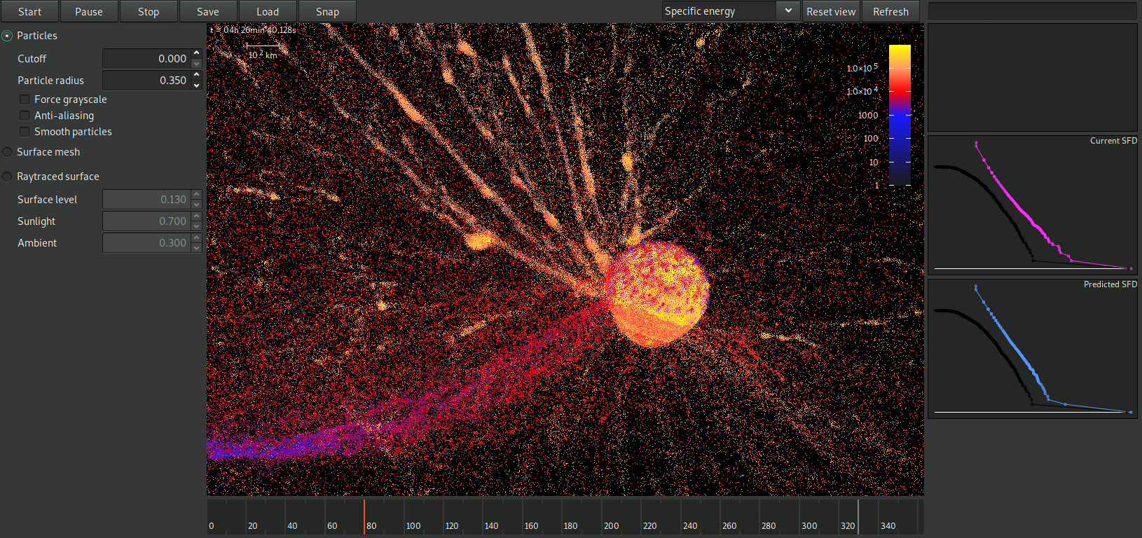
Figure 10: Screenshot of the graphical interface of our code.

References

- Ballouz et al. (2015) Ballouz, R.L., Richardson, D.C., Michel, P., Schwartz, S.R., Yu, Y., 2015. Numerical simulations of collisional disruption of rotating gravitational aggregates: Dependence on material properties. LABEL:@jnlPlanet. Space Sci. 107, 29–35. doi:, arXiv:1409.6650.
- Ballouz et al. (2018) Ballouz, R.L., Walsh, K.J., Richardson, D.C., Michel, P., 2018. Numerical Simulations of Asteroid Reaccumulation: Improving the SPH to N-Body Handoff Using Alpha Shapes, in: Lunar and Planetary Science Conference, p. 2816.
- Balsara (1995) Balsara, D.S., 1995. von Neumann stability analysis of smoothed particle hydrodynamics—suggestions for optimal algorithms. Journal of Computational Physics 121, 357–372. doi:.
- Barnes and Hut (1986) Barnes, J., Hut, P., 1986. A hierarchical O(N log N) force-calculation algorithm. Nature 324, 446–449. doi:.
- Benavidez et al. (2018) Benavidez, P.G., Durda, D.D., Enke, B., Campo Bagatin, A., Richardson, D.C., Asphaug, E., Bottke, W.F., 2018. Impact simulation in the gravity regime: Exploring the effects of parent body size and internal structure. Icarus 304, 143–161. doi:.
- Benavidez et al. (2012) Benavidez, P.G., Durda, D.D., Enke, B.L., Bottke, W.F., Nesvorný, D., Richardson, D.C., Asphaug, E., Merline, W.J., 2012. A comparison between rubble-pile and monolithic targets in impact simulations: Application to asteroid satellites and family size distributions. Icarus 219, 57–76. doi:.
- Benz and Asphaug (1994) Benz, W., Asphaug, E., 1994. Impact simulations with fracture. I - Method and tests. Icarus 107, 98. doi:.
- Benz and Asphaug (1999) Benz, W., Asphaug, E., 1999. Catastrophic Disruptions Revisited. Icarus 142, 5–20. doi:, arXiv:arXiv:astro-ph/9907117.
- Canup (2005) Canup, R.M., 2005. A Giant Impact Origin of Pluto-Charon. Science 307, 546–550. doi:.
- Canup (2008) Canup, R.M., 2008. Lunar-forming collisions with pre-impact rotation. Icarus 196, 518–538. doi:.
- Cossins (2010) Cossins, P.J., 2010. The Gravitational Instability and its Role in the Evolution of Protostellar and Protoplanetary Discs. Ph.D. thesis. University of Leicester.
- Ćuk and Stewart (2012) Ćuk, M., Stewart, S.T., 2012. Making the Moon from a Fast-Spinning Earth: A Giant Impact Followed by Resonant Despinning. Science 338, 1047. doi:.
- Dahlgren (1998) Dahlgren, M., 1998. A study of Hilda asteroids. III. Collision velocities and collision frequencies of Hilda asteroids. A&A 336, 1056–1064.
- Dobrovolskis and Burns (1984) Dobrovolskis, A.R., Burns, J.A., 1984. Angular momentum drain - A mechanism for despinning asteroids. Icarus 57, 464–476. doi:.
- Durda et al. (2007) Durda, D.D., Bottke, W.F., Nesvorný, D., Enke, B.L., Merline, W.J., Asphaug, E., Richardson, D.C., 2007. Size-frequency distributions of fragments from SPH/N-body simulations of asteroid impacts: Comparison with observed asteroid families. Icarus 186, 498–516. doi:.
- Fétick et al. (2019) Fétick, R.J., Jorda, L., Vernazza, P., Marsset, M., Drouard, A., Fusco, T., Carry, B., Marchis, F., Hanuš, J., Viikinkoski, M., Birlan, M., Bartczak, P., Berthier, J., Castillo-Rogez, J., Cipriani, F., Colas, F., Dudziński, G., Dumas, C., Ferrais, M., Jehin, E., Kaasalainen, M., Kryszczynska, A., Lamy, P., Le Coroller, H., Marciniak, A., Michalowski, T., Michel, P., Mugnier, L.M., Neichel, B., Pajuelo, M., Podlewska-Gaca, E., Santana-Ros, T., Tanga, P., Vachier, F., Vigan, A., Witasse, O., Yang, B., 2019. Closing the gap between Earth-based and interplanetary mission observations: Vesta seen by VLT/SPHERE. A&A 623, A6. doi:, arXiv:1902.01287.
- Hirabayashi and Scheeres (2014) Hirabayashi, M., Scheeres, D.J., 2014. Analysis of Asteroid (216) Kleopatra Using Dynamical and Structural Constraints. ApJ 780, 160. doi:, arXiv:1312.4976.
- Jutzi et al. (2013) Jutzi, M., Asphaug, E., Gillet, P., Barrat, J.A., Benz, W., 2013. The structure of the asteroid 4 Vesta as revealed by models of planet-scale collisions. Nature 494, 207–210. doi:.
- Jutzi and Benz (2017) Jutzi, M., Benz, W., 2017. Formation of bi-lobed shapes by sub-catastrophic collisions. A late origin of comet 67P’s structure. A&A 597, A62. doi:, arXiv:1611.02615.
- Jutzi et al. (2015) Jutzi, M., Holsapple, K., Wünneman, K., Michel, P., 2015. Modeling asteroid collisions and impact processes, in: Michel, P., DeMeo, F.E., Bottke, W.F. (Eds.), Asteroids IV. The University of Arizona Press, pp. 679–699.
- Jutzi et al. (2019) Jutzi, M., Michel, P., Richardson, D.C., 2019. Fragment properties from large-scale asteroid collisions: I: Results from SPH/N-body simulations using porous parent bodies and improved material models. Icarus 317, 215–228. doi:, arXiv:1808.03464.
- Kurosawa and Genda (2018) Kurosawa, K., Genda, H., 2018. Effects of Friction and Plastic Deformation in Shock-Comminuted Damaged Rocks on Impact Heating. Geochim. Res. Lett. 45, 620–626. doi:, arXiv:1801.01100.
- Marrone et al. (2011) Marrone, S., Antuono, M., Colagrossi, A., Colicchio, G., Touzé, D.L., Graziani, G., 2011. -sph model for simulating violent impact flows. Computer Methods in Applied Mechanics and Engineering 200, 1526 – 1542. doi:.
- Michel and Richardson (2013) Michel, P., Richardson, D.C., 2013. Collision and gravitational reaccumulation: Possible formation mechanism of the asteroid Itokawa. A&A 554, L1. doi:.
- Michel et al. (2015) Michel, P., Richardson, D.C., Durda, D.D., Jutzi, M., Asphaug, E., 2015. Collisional Formation and Modeling of Asteroid Families, in: Michel, P., DeMeo, F.E., Bottke, W.F. (Eds.), Asteroids IV. The University of Arizona Press, pp. 341–354. doi:.
- Monaghan and Gingold (1983) Monaghan, J., Gingold, R., 1983. Shock simulation by the particle method sph. Journal of Computational Physics 52, 374 – 389. doi:.
- Monaghan (1985) Monaghan, J.J., 1985. Particle methods for hydrodynamics. Computer Physics Reports 3, 71–124. doi:.
- Monaghan (2000) Monaghan, J.J., 2000. SPH without a Tensile Instability. Journal of Computational Physics 159, 290–311. doi:.
- Morris and Burchell (2017) Morris, A.J.W., Burchell, M.J., 2017. Laboratory tests of catastrophic disruption of rotating bodies. Icarus 296, 91–98. doi:.
- Nakamura and Fujiwara (1991) Nakamura, A., Fujiwara, A., 1991. Velocity distribution of fragments formed in a simulated collisional disruption. Icarus 92, 132–146. doi:.
- Nesvorný et al. (2015) Nesvorný, D., Brož, M., Carruba, V., 2015. Identification and Dynamical Properties of Asteroid Families, in: Michel, P., DeMeo, F.E., Bottke, W.F. (Eds.), Asteroids IV. The University of Arizona Press, pp. 297–321.
- Owen (2014) Owen, J.M., 2014. A compatibly differenced total energy conserving form of SPH. International Journal for Numerical Methods in Fluids 75, 749–774. doi:.
- Reinhardt and Stadel (2017) Reinhardt, C., Stadel, J., 2017. Numerical aspects of giant impact simulations. MNRAS 467, 4252–4263. doi:, arXiv:1701.08296.
- Remington et al. (2018) Remington, T., Owen, J.M., Nakamura, A., Miller, P.L., Bruck Syal, M., 2018. Benchmarking Asteroid-Deflection Simulations: Basalt Spheres, in: AAS/Division for Planetary Sciences Meeting Abstracts #50, p. 312.02.
- Richardson et al. (2000) Richardson, D.C., Quinn, T., Stadel, J., Lake, G., 2000. Direct Large-Scale N-Body Simulations of Planetesimal Dynamics. Icarus 143, 45–59. doi:.
- Schäfer et al. (2016) Schäfer, C., Riecker, S., Maindl, T.I., Speith, R., Scherrer, S., Kley, W., 2016. A smooth particle hydrodynamics code to model collisions between solid, self-gravitating objects. A&A 590, A19. doi:, arXiv:1604.03290.
- Ševeček et al. (2017) Ševeček, P., Brož, M., Nesvorný, D., Enke, B., Durda, D., Walsh, K., Richardson, D.C., 2017. SPH/N-Body simulations of small (D = 10km) asteroidal breakups and improved parametric relations for Monte-Carlo collisional models. Icarus 296, 239–256. doi:.
- Stadel (2001) Stadel, J.G., 2001. Cosmological N-body simulations and their analysis. Ph.D. thesis. University of Washington.
- Suetsugu et al. (2018) Suetsugu, R., Tanaka, H., Kobayashi, H., Genda, H., 2018. Collisional disruption of planetesimals in the gravity regime with iSALE code: Comparison with SPH code for purely hydrodynamic bodies. Icarus 314, 121–132. doi:, arXiv:1805.11755.
- Sugiura et al. (2018) Sugiura, K., Kobayashi, H., Inutsuka, S., 2018. Toward understanding the origin of asteroid geometries. Variety in shapes produced by equal-mass impacts. A&A 620, A167. doi:, arXiv:1804.11039.
- Takeda and Ohtsuki (2007) Takeda, T., Ohtsuki, K., 2007. Mass dispersal and angular momentum transfer during collisions between rubble-pile asteroids. Icarus 189, 256–273. doi:.
- Takeda and Ohtsuki (2009) Takeda, T., Ohtsuki, K., 2009. Mass dispersal and angular momentum transfer during collisions between rubble-pile asteroids. II. Effects of initial rotation and spin-down through disruptive collisions. Icarus 202, 514–524. doi:.
- Tillotson (1962) Tillotson, J.H., 1962. Metallic equations of state for hypervelocity impact. General Atomic Report GA-3216.
- Vernazza et al. (2018) Vernazza, P., Brož, M., Drouard, A., Hanuš, J., Viikinkoski, M., Marsset, M., Jorda, L., Fetick, R., Carry, B., Marchis, F., Birlan, M., Fusco, T., Santana-Ros, T., Podlewska-Gaca, E., Jehin, E., Ferrais, M., Bartczak, P., Dudziński, G., Berthier, J., Castillo-Rogez, J., Cipriani, F., Colas, F., Dumas, C., Ďurech, J., Kaasalainen, M., Kryszczynska, A., Lamy, P., Le Coroller, H., Marciniak, A., Michalowski, T., Michel, P., Pajuelo, M., Tanga, P., Vachier, F., Vigan, A., Warner, B., Witasse, O., Yang, B., Asphaug, E., Richardson, D.C., Ševeček, P., Gillon, M., Benkhaldoun, Z., 2018. The impact crater at the origin of the Julia family detected with VLT/SPHERE? A&A 618, A154. doi:.
- Vinogradova (2019) Vinogradova, T.A., 2019. Empirical method of proper element calculation and identification of asteroid families. MNRAS 484, 3755–3764. doi:.
- Wickham-Eade et al. (2018) Wickham-Eade, J.E., Burchell, M.J., Price, M.C., Harriss, K.H., 2018. Hypervelocity impact fragmentation of basalt and shale projectiles. Icarus 311, 52–68. doi:.