Key Fact as Pivot: A Two-Stage Model for Low Resource
Table-to-Text Generation

Abstract

Table-to-text generation aims to translate the structured data into the unstructured text. Most existing methods adopt the encoder-decoder framework to learn the transformation, which requires large-scale training samples. However, the lack of large parallel data is a major practical problem for many domains. In this work, we consider the scenario of low resource table-to-text generation, where only limited parallel data is available. We propose a novel model to separate the generation into two stages: key fact prediction and surface realization. It first predicts the key facts from the tables, and then generates the text with the key facts. The training of key fact prediction needs much fewer annotated data, while surface realization can be trained with pseudo parallel corpus. We evaluate our model on a biography generation dataset. Our model can achieve $27.34$ BLEU score with only $1,000$ parallel data, while the baseline model only obtain the performance of $9.71$ BLEU score.

1 Introduction

Table-to-text generation is to generate a description from the structured table. It helps readers to summarize the key points in the table, and tell in the natural language. Figure 1 shows an example of table-to-text generation. The table provides some structured information about a person named “Denise Margaret Scott”, and the corresponding text describes the person with the key information in the table. Table-to-text generation can be applied in many scenarios, including weather report generation Liang et al. (2009), NBA news writing Barzilay and Lapata (2005), biography generation Duboué and McKeown (2002); Lebret et al. (2016), and so on. Moreover, table-to-text generation is a good testbed of a model’s ability of understanding the structured knowledge.

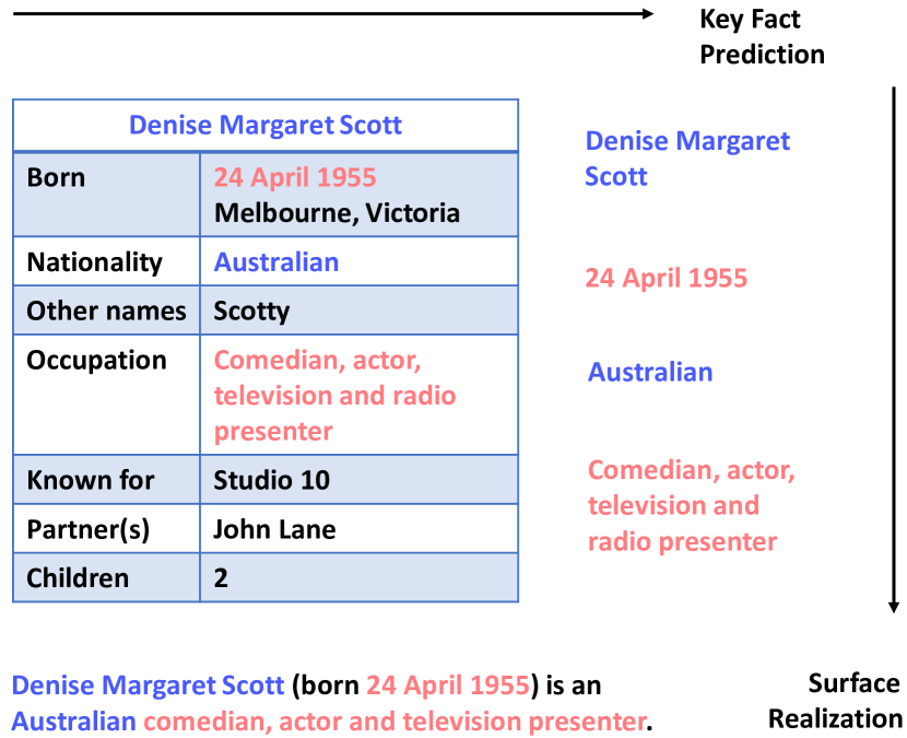
Figure 1: An example of table-to-text generation, and also a flow chart of our method.

Most of the existing methods for table-to-text generation are based on the encoder-decoder framework Sutskever et al. (2014); Bahdanau et al. (2014). They represent the source tables with a neural encoder, and generate the text word-by-word with a decoder conditioned on the source table representation. Although the encoder-decoder framework has proven successful in the area of natural language generation (NLG) Luong et al. (2015); Chopra et al. (2016); Lu et al. (2017); Yang et al. (2018), it requires a large parallel corpus, and is known to fail when the corpus is not big enough. Figure 2 shows the performance of a table-to-text model trained with different number of parallel data under the encoder-decoder framework. We can see that the performance is poor when the parallel data size is low. In practice, we lack the large parallel data in many domains, and it is expensive to construct a high-quality parallel corpus.

This work focuses on the task of low resource table-to-text generation, where only limited parallel data is available. Some previous work (Puduppully et al., 2018; Gehrmann et al., 2018) formulates the task as the combination of content selection and surface realization, and models them with an end-to-end model. Inspired by these work, we break up the table-to-text generation into two stages, each of which is performed by a model trainable with only a few annotated data. Specifically, it first predicts the key facts from the tables, and then generates the text with the key facts, as shown in Figure 1. The two-stage method consists of two separate models: a key fact prediction model and a surface realization model. The key fact prediction model is formulated as a sequence labeling problem, so it needs much fewer annotated data than the encoder-decoder models. According to our experiments, the model can obtain $87.92\%$ F1 score with only $1,000$ annotated data. As for the surface realization model, we propose a method to construct a pseudo parallel dataset without the need of labeled data. In this way, our model can make full use of the unlabeled text, and alleviate the heavy need of the parallel data.

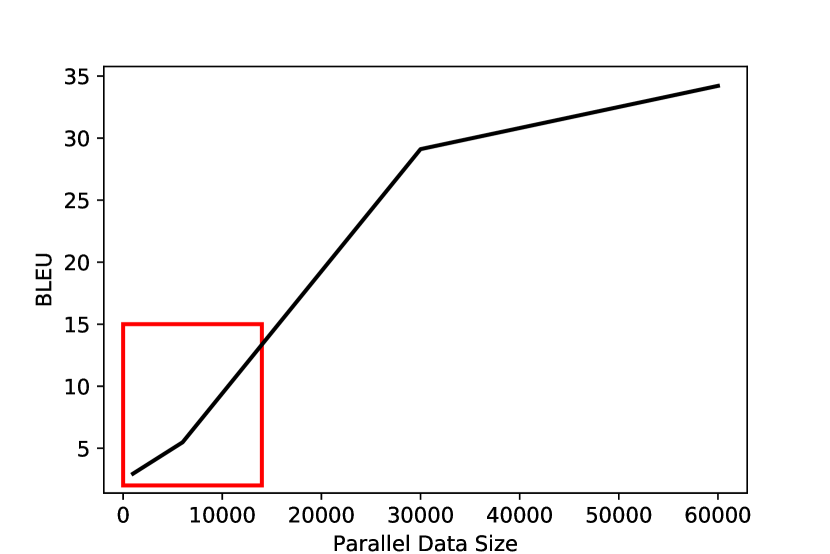
Figure 2: The BLEU scores of the a table-to-text model trained with different number of parallel data under the encoder-decoder framework on the WIKIBIO dataset.

The contributions of this work are as follows:

• We propose to break up the table-to-text generation into two stages with two separate models, so that the model can be trained with fewer annotated data.

• We propose a method to construct a pseudo parallel dataset for the surface realization model, without the need of labeled data.

• Experiments show that our proposed model can achieve $27.34$ BLEU score on a biography generation dataset with only $1,000$ table-text samples.

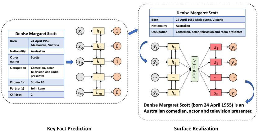
Figure 3: The overview of our model. For illustration, the surface realization model is a vanilla Seq2Seq, while it can also be a Transformer in our implementation.

2 Pivot: A Two-Stage Model

In this section, we introduce our proposed two-stage model, which we denote as Pivot. We first give the formulation of the table-to-text generation and the related notations. Then, we provide an overview of the model. Finally, we describe the two models for each stage in detail.

2.1 Formulation and Notations

Suppose we have a parallel table-to-text dataset $\mathcal{P}$ with $N$ data samples and an unlabeled text dataset $\mathcal{U}$ with $M$ samples. Each parallel sample consists of a source table $T$ and a text description $\bm{y}=\{y_{1},y_{2},\cdots,y_{n}\}$. The table $T$ can be formulated as $K$ records $T=\{r_{1},r_{2},r_{3},\cdots,r_{K}\}$, and each record is an attribute-value pair $r_{j}=(a_{j},v_{j})$. Each sample in the unlabeled text dataset $\mathcal{U}$ is a piece of text $\bm{\bar{y}}=\{\bar{y}_{1},\bar{y}_{2},\cdots,\bar{y}_{n}\}$.

Formally, the task of table-to-text generation is to take the structured representations of table $T=\{(a_{1},v_{1}),(a_{2},v_{2}),\cdots,(a_{m},v_{m})\}$ as input, and output the sequence of words $\bm{y}=\{y_{1},y_{2},\cdots,y_{n}\}$.

2.2 Overview

Figure 3 shows the overview architecture of our proposed model. Our model contains two stages: key fact prediction and surface realization. At the first stage, we represent the table into a sequence, and use a table-to-pivot model to select the key facts from the sequence. The table-to-pivot model adpots a bi-directional Long Short-term Memory Network (Bi-LSTM) to predict a binary sequence of whether each word is reserved as the key facts. At the second stage, we build a sequence-to-sequence model to take the key facts selected in the first stage as input and emit the table description. In order to make use of the unlabeled text corpus, we propose a method to construct pseudo parallel data to train a better surface realization model. Moreover, we introduce a denoising data augmentation method to reduce the risk of error propagation between two stages.

2.3 Preprocessing: Key Fact Selection

The two stages are trained separately, but we do not have the labels of which words in the table are the key facts in the dataset. In this work, we define the co-occurrence facts between the table and the text as the key facts, so we can label the key facts automatically. Algorithm 1 illustrates the process of automatically annotating the key facts. Given a table and its associated text, we enumerate each attribute-value pair in the table, and compute the word overlap between the value and the text. The word overlap is defined as the number of words that are not stop words or punctuation but appear in both the table and the text. We collect all values that have at least one overlap with the text, and regard them as the key facts. In this way, we can obtain a binary sequence with the $0/1$ label denoting whether the values in the table are the key facts. The binary sequence will be regarded as the supervised signal of the key fact prediction model, and the selected key facts will be the input of the surface realization model.

Algorithm 1 Automatic Key Fact Annotation

1:A parallel corpora $\mathcal{P}=\{(\bm{x}_{i},\bm{y}_{i})\}$, where $\bm{x}_{i}$ is a table, and $\bm{y}_{i}$ is a word sequence.

2:Initial the selected key fact list $\mathbb{W}=[]$

3:for each sample $(\bm{x},\bm{y})$ in the parallel dataset $\mathcal{P}$ do

4:     $\bm{x}=\{(v_{1},a_{1}),(v_{2},a_{2}),\cdots,(v_{m},a_{m})\}$

5:     $\bm{y}=\{y_{1},y_{2},\cdots,y_{n}\}$

6:     Initial the selected attribute set $\mathbb{A}=\{\}$

7:     Initial the selected key fact list $\mathbb{W}_{i}=[]$

8:     for each attribute-value pair $(v_{i},a_{i})$ in table $\bm{x}$ do

9:         if $v_{i}$ in $\bm{y}$ And $v_{i}$ is not stop word then

10:              Append attribute $a_{i}$ into attribute set $\mathbb{A}$

11:         end if

12:         if $a_{i}$ in $\mathbb{A}$ then

13:              Append value $v_{i}$ into key fact list $\mathbb{W}_{i}$

14:         end if

15:     end for

16:     Collect the key fact list $\mathbb{W}$ += $\mathbb{W}_{i}$

17:end for

18:The selected key fact list $\mathbb{W}$

2.4 Stage 1: Key Fact Prediction

The key fact prediction model is a Bi-LSTM layer with a multi-layer perceptron (MLP) classifier to determine whether each word is selected. In order to represent the table, we follow the previous work Liu et al. (2018) to concatenate all the words in the values of the table into a word sequence, and each word is labeled with its attribute. In this way, the table is represented as two sequences: the value sequence $\{v_{1},v_{2},\cdots,v_{m}\}$ and the attribute sequence $\{a_{1},a_{2},\cdots,a_{m}\}$. A word embedding and an attribute embedding are used to transform two sequences into the vectors. Following Lebret et al. (2016); Liu et al. (2018), we introduce a position embedding to capture structured information of the table. The position information is represented as a tuple ($p^{+}_{w}$, $p^{−}_{w}$), which includes the positions of the token $w$ counted from the beginning and the end of the value respectively. For example, the record of “(Name, Denise Margaret Scott)” is represented as “({Denise, Name, 1, 3}, {Margaret, Name, 2, 2}, {Scott, Name, 3, 1})”. In this way, each token in the table has an unique feature embedding even if there exists two same words. Finally, the word embedding, the attribute embedding, and the position embedding are concatenated as the input of the model $\bm{x}$.

Table Encoder: The goal of the source table encoder is to provide a series of representations for the classifier. More specifically, the table encoder is a Bi-LSTM:

$$h_{t}=\mathrm{BiLSTM}(x_{t},\vec{h}_{t-1},\reflectbox{$\vec{\reflectbox{$h$}}$}_{t+1})$$ (1)

where $\vec{h}_{t}$ and $\reflectbox{$\vec{\reflectbox{$h$}}$}_{t}$ are the forward and the backward hidden outputs respectively, $h_{t}$ is the concatenation of $\vec{h}_{t}$ and $\reflectbox{$\vec{\reflectbox{$h$}}$}_{t}$, and $x_{t}$ is the input at the $t$-th time step.

Classifier: The output vector $h_{t}$ is fed into a MLP classifier to compute the probability distribution of the label $p_{1}(l_{t}|\bm{x})$

$$p_{1}(l_{t}|\bm{x})=\mathrm{softmax}{(W_{c}h_{t}+b_{c})}$$ (2)

where $W_{c}$ and $b_{c}$ are trainable parameters of the classifier.

2.5 Stage 2: Surface Realization

The surface realization stage aims to generate the text conditioned on the key facts predicted in Stage 1. We adpot two models as the implementation of surface realization: the vanilla Seq2Seq and the Transformer Vaswani et al. (2017).

Vanilla Seq2Seq:

In our implementation, the vanilla Seq2Seq consists of a Bi-LSTM encoder and an LSTM decoder with the attention mechanism. The Bi-LSTM encoder is the same as that of the key fact prediction model, except that it does not use any attribute embedding or position embedding.

The decoder consists of an LSTM, an attention component, and a word generator. It first generates the hidden state $s_{t}$:

$$s_{t}=f(y_{t-1},s_{t-1})$$ (3)

where $f(\cdot,\cdot)$ is the function of LSTM for one time step, and $y_{t-1}$ is the last generated word at time step $t-1$. Then, the hidden state $s_{t}$ from LSTM is fed into the attention component:

$$v_{t}=\mathrm{Attention}({s_{t},\bm{h}})$$ (4)

where $\mathrm{Attention}(\cdot,\cdot)$ is the implementation of global attention in (Luong et al., 2015), and $\bm{h}$ is a sequence of outputs by the encoder.

Given the output vector $v_{t}$ from the attention component, the word generator is used to compute the probability distribution of the output words at time step $t$:

$$p_{2}(y_{t}|x)=\mathrm{softmax}{(W_{g}v_{t}+b_{g})}$$ (5)

where $W_{g}$ and $b_{g}$ are parameters of the generator. The word with the highest probability is emitted as the $t$-th word.

Transformer:

Similar to vanilla Seq2Seq, the Transformer consists of an encoder and a decoder. The encoder applies a Transformer layer to encode each word into the representation $h_{t}$:

$$h_{t}=\mathrm{Transformer}(x_{t},\bm{x})$$ (6)

Inside the Transformer, the representation $x_{t}$ attends to a collection of the other representations $\bm{x}=\{x_{1},x_{2},\cdots,x_{m}\}$. Then, the decoder produces the hidden state by attending to both the encoder outputs and the previous decoder outputs:

$$v_{t}=\mathrm{Transformer}(y_{t},\bm{y_{<t}},\bm{h})$$ (7)

Finally, the output vector is fed into a word generator with a softmax layer, which is the same as Eq. 5.

For the purpose of simplicity, we omit the details of the inner computation of the Transformer layer, and refer the readers to the related work Vaswani et al. (2017).

2.6 Pseudo Parallel Data Construction

The surface realization model is based on the encoder-decoder framework, which requires a large amount of training data. In order to augment the training data, we propose a novel method to construct pseudo parallel data. The surface realization model is used to organize and complete the text given the key facts. Therefore, it is possible to construct the pseudo parallel data by removing the skeleton of the text and reserving only the key facts. In implementation, we label the text with Stanford CoreNLP toolkit to assign the POS tag for each word. We reserve the words whose POS tags are among the tag set of {NN, NNS, NNP, NNPS, JJ, JJR, JJS, CD, FW}, and remove the remaining words. In this way, we can construct a large-scale pseudo parallel data to train the surface realization model.

2.7 Denoising Data Augmentation

A problem of the two-stage model is that the error may propagate from the first stage to the second stage. A possible solution is to apply beam search to enlarge the searching space at the first stage. However, in our preliminary experiments, when the beam size is small, the diversity of predicted key facts is low, and also does not help to improve the accuracy. When the beam size is big, the decoding speed is slow but the improvement of accuracy is limited.

To address this issue, we implement a method of denoising data augmentation to reduce the hurt from error propagation and improve the robustness of our model. In practice, we randomly drop some words from the input of surface realization model, or insert some words from other samples. The dropping simulates the cases when the key fact prediction model fails to recall some co-occurrence, while the inserting simulates the cases when the model predicts some extra facts from the table. By adding the noise, we can regard these data as the adversarial examples, which is able to improve the robustness of the surface realization model.

2.8 Training and Decoding

Since the two components of our model are separate, the objective functions of the models are optimized individually.

Training of Key Fact Prediction Model:

The key fact prediction model, as a sequence labeling model, is trained using the cross entropy loss:

$$L_{1}=-\sum_{i=1}^{m}\log p_{1}(l_{i}|\bm{x})$$ (8)

Training of Surface Realization Model:

The loss function of the surface realization model can be written as:

$$L_{2}=-\sum_{i=1}^{n}\log p_{2}(y_{i}|\bm{\bar{x}})$$ (9)

where $\bm{\bar{x}}$ is a sequence of the selected key facts at Stage 1. The surface realization model is also trained with the pseudo parallel data as described in Section 2.6. The objective function can be written as:

$$L_{3}=-\sum_{i=1}^{n}\log p_{2}(\bar{y}_{i}|\bm{\hat{x}})$$ (10)

where $\bar{y}$ is the unlabeled text, and $\bm{\hat{x}}$ is the pseudo text paired with $\bar{y}$.

Decoding:

The decoding consists of two steps. At the first step, it predicts the label by the key fact prediction model:

$$\hat{l}_{t}=\operatorname*{arg\,max}_{l_{t}\in\{0,1\}}{p_{1}(l_{t}|\bm{x})}$$ (11)

The word with $\hat{l}_{t}=1$ is reserved, while that with $\hat{l}_{t}=0$ is discarded. Therefore, we can obtain a sub-sequence $\bm{\bar{x}}$ after the discarding operation.

At the second step, the model emits the text with the surface realization model:

$$\hat{y}_{t}=\operatorname*{arg\,max}_{y_{t}\in\mathcal{V}}p_{2}(y_{t}|\bm{\bar{x}})$$ (12)

where $\mathcal{V}$ is the vocabulary size of the model. Therefore, the word sequence $\{\hat{y}_{1},\hat{y}_{2},\cdots,\hat{y}_{N}\}$ forms the generated text.

3 Experiments

We evaluate our model on a table-to-text generation benchmark. We denote the Pivot model under the vanilla Seq2Seq framework as Pivot-Vanilla, and that under the Transformer framework as Pivot-Trans.

3.1 Dataset

We use WIKIBIO dataset (Lebret et al., 2016) as our benchmark dataset. The dataset contains $728,321$ articles from English Wikipedia, which uses the first sentence of each article as the description of the related infobox. There are an average of $26.1$ words in each description, of which $9.5$ words also appear in the table. The table contains $53.1$ words and $19.7$ attributes on average. Following the previous work (Lebret et al., 2016; Liu et al., 2018), we split the dataset into $80\%$ training set, $10\%$ testing set, and $10\%$ validation set. In order to simulate the low resource scenario, we randomly sample $1,000$ parallel sample, and remove the tables from the rest of the training data.

3.2 Evaluation Metrics

Following the previous work (Lebret et al., 2016; Wiseman et al., 2018), we use BLEU-4 (Papineni et al., 2002), ROUGE-4 (F measure) (Lin and Hovy, 2003), and NIST-4 (Belz and Reiter, 2006) as the evaluation metrics.

3.3 Implementation Details

The vocabulary is limited to the $20,000$ most common words in the training dataset. The batch size is $64$ for all models. We implement the early stopping mechanism with a patience that the performance on the validation set does not fall in $4$ epochs. We tune the hyper-parameters based on the performance on the validation set.

The key fact prediction model is a Bi-LSTM. The dimensions of the hidden units, the word embedding, the attribute embedding, and the position embedding are $500$, $400$, $50$, and $5$, respectively.

We implement two models as the surface realization models. For the vanilla Seq2Seq model, we set the hidden dimension, the embedding dimension, and the dropout rate (Srivastava et al., 2014) to be $500$, $400$, and $0.2$, respectively. For the Transfomer model, the hidden units of the multi-head component and the feed-forward layer are $512$ and $2048$. The embedding size is $512$, the number of heads is $8$, and the number of Transformer blocks is $6$.

We use the Adam Kingma and Ba (2014) optimizer to train the models. For the hyper-parameters of Adam optimizer, we set the learning rate $\alpha=0.001$, two momentum parameters $\beta_{1}=0.9$ and $\beta_{2}=0.999$, and $\epsilon=1\times 10^{-8}$. We clip the gradients Pascanu et al. (2013) to the maximum norm of $5.0$. We half the learning rate when the performance on the validation set does not improve in $3$ epochs.

3.4 Baselines

We compare our models with two categories of baseline models: the supervised models which exploit only parallel data (Vanilla Seq2Seq, Transformer, Struct-aware), and the semi-supervised models which are trained on both parallel data and unlabelled data (PretrainedMT, SemiMT). The baselines are as follows:

• Vanilla Seq2Seq (Sutskever et al., 2014) with the attention mechanism (Bahdanau et al., 2014) is a popular model for natural language generation.

• Transformer (Vaswani et al., 2017) is a state-of-the-art model under the encoder-decoder framework, based solely on attention mechanisms.

• Struct-aware (Liu et al., 2018) is the state-of-the-art model for table-to-text generation. It models the inner structure of table with a field-gating mechanism insides the LSTM, and learns the interaction between tables and text with a dual attention mechanism.

• PretrainedMT (Skorokhodov et al., 2018) is a semi-supervised method to pretrain the decoder of the sequence-to-sequence model with a language model.

• SemiMT (Cheng et al., 2016) is a semi-supervised method to jointly train the sequence-to-sequence model with an auto-encoder.

The supervised models are trained with the same parallel data as our model, while the semi-supervised models share the same parallel data and the unlabeled data as ours.

Model	F1	P	R
Pivot (Bi-LSTM)	$87.92$	92.59	$83.70$
Model	BLEU	NIST	ROUGE
Vanilla Seq2Seq	$2.14$	0.2809	$0.47$
Structure-S2S	$3.27$	0.9612	$0.71$
PretrainedMT	$4.35$	1.9937	$0.91$
SemiMT	$6.76$	3.5017	$2.04$
Pivot-Vanilla	$20.09$	6.5130	$18.31$
Model	BLEU	NIST	ROUGE
Transformer	$5.48$	1.9873	$1.26$
PretrainedMT	$6.43$	2.1019	$1.77$
SemiMT	$9.71$	2.7019	$3.31$
Pivot-Trans	$27.34$	6.8763	$19.30$

Table 1: Results of our model and the baselines. Above is the performance of the key fact prediction component (F1: F1 score, P: precision, R: recall). Middle is the comparison between models under the Vanilla Seq2Seq framework. Below is the models implemented with the transformer framework.

3.5 Results

We compare our Pivot model with the above baseline models. Table 1 summarizes the results of these models. It shows that our Pivot model achieves $87.92\%$ F1 score, $92.59\%$ precision, and $83.70\%$ recall at the stage of key fact prediction, which provides a good foundation for the stage of surface realization. Based on the selected key facts, our models achieve the scores of $20.09$ BLEU, $6.5130$ NIST, and $18.31$ ROUGE under the vanilla Seq2Seq framework, and $27.34$ BLEU, $6.8763$ NIST, and $19.30$ ROUGE under the Transformer framework, which significantly outperform all the baseline models in terms of all metrics. Furthermore, it shows that the implementation with the Transformer can obtain higher scores than that with the vanilla Seq2Seq.

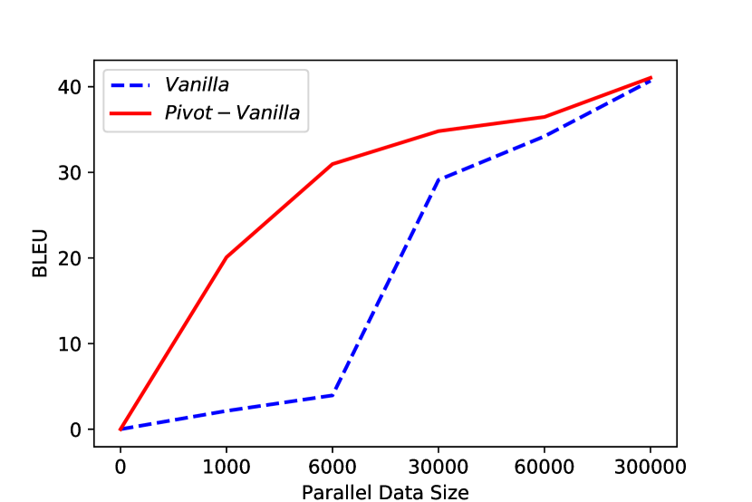
(a) Vanilla Seq2Seq v.s Pivot-Vanilla

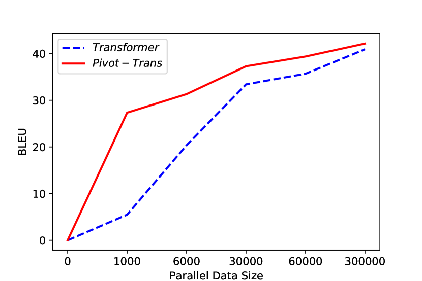
(b) Transformer v.s Pivot-Trans

Figure 4: The BLEU measure of our Pivot model and the baselines trained with different parallel data size.

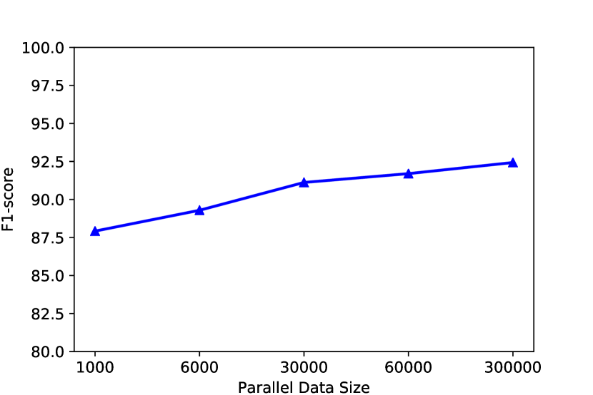
Figure 5: The F1 score of the key fact prediction model trained with different parallel data size.

Model	BLEU	NIST	ROUGE
Vanilla Seq2Seq	$2.14$	$0.2809$	$0.47$
+ Pseudo	$10.01$	$3.0620$	$6.55$
Transformer	$6.43$	$2.1019$	$1.77$
+ Pseudo	$14.35$	$4.1763$	$8.42$
w/o Pseudo	$11.08$	$3.6910$	$4.84$
Pivot-Vanilla	$20.09$	$6.5130$	$18.31$
w/o Pseudo	$14.18$	$4.2686$	$7.10$
Pivot-Trans	$27.34$	$6.8763$	$19.30$

Table 2: Ablation study on the 1k training set for the effect of pseudo parallel data.

Model	BLEU	NIST	ROUGE
Pivot-Vanilla	$20.09$	$6.5130$	$18.31$
w/o denosing	$18.45$	$4.8714$	$11.43$
Pivot-Trans	$27.34$	$6.8763$	$19.30$
w/o denosing	$25.72$	$6.5475$	$17.95$

Table 3: Ablation study on the 1k training set for the effect of the denoising data augmentation.

3.6 Varying Parallel Data Size

We would like to further analyze the performance of our model given different size of parallel size. Therefore, we randomly shuffle the full parallel training set. Then, we extract the first $K$ samples as the parallel data, and modify the remaining data as the unlabeled data by removing the tables. We set $K=1000,6000,30000,60000,300000$, and compare our pivot models with both vanilla Seq2Seq and Transformer. Figure 4 shows the BLEU scores of our models and the baselines. When the parallel data size is small, the pivot model can outperform the vanilla Seq2Seq and Transformer by a large margin. With the increasement of the parallel data, the margin gets narrow because of the upper bound of the model capacity. Figure 5 shows the curve of the F1 score of the key fact prediction model trained with different parallel data size. Even when the number of annotated data is extremely small, the model can obtain a satisfying F1 score about $88\%$. In general, the F1 scores between the low and high parallel data sizes are close, which validates the assumption that the key fact prediction model does not rely on a heavy annotated data.

3.7 Effect of Pseudo Parallel Data

In order to analyze the effect of pseudo parallel data, we conduct ablation study by adding the data to the baseline models and removing them from our models. Table 2 summarizes the results of the ablation study. Surprisingly, the pseudo parallel data can not only help the pivot model, but also significantly improve vanilla Seq2Seq and Transformer. The reason is that the pseudo parallel data can help the models to improve the ability of surface realization, which these models lack under the condition of limited parallel data. The pivot models can outperform the baselines with pseudo data, mainly because it breaks up the operation of key fact prediction and surface realization, both of which are explicitly and separately optimized.

3.8 Effect of Denoising Data Augmentation

We also want to know the effect of the denoising data augmentation. Therefore, we remove the denoising data augmentation from our model, and compare with the full model. Table 3 shows the results of the ablation study. It shows that the data augmentation brings a significant improvement to the pivot models under both vanilla Seq2Seq and Transformer frameworks, which demonstrates the efficiency of the denoising data augmentation.

Transformer: a athletics -lrb- nfl -rrb- .
SemiMT: gustav dovid -lrb- born 25 august 1945 -rrb- is a former hungarian politician , who served as a member of the united states -lrb- senate -rrb- from president to 1989 .
Pivot-Trans: philippe adnot -lrb- born august 25 , 1945 -rrb- is a french senator , senator , and a senator of the french senate .
Reference: philippe adnot -lrb- born 25 august 1945 in rhèges -rrb- is a member of the senate of france .

Table 4: An example of the generated text by our model and the baselines on 1k training set.

3.9 Qualitative Analysis

We provide an example to illustrate the improvement of our model more intuitively, as shown in Table 4. Under the low resource setting, the Transformer can not produce a fluent sentence, and also fails to select the proper fact from the table. Thanks to the unlabeled data, the SemiMT model can generate a fluent, human-like description. However, it suffers from the hallucination problem so that it generates some unseen facts, which is not faithful to the source input. Although the Pivot model has some problem in generating repeating words (such as “senator” in the example), it can select the correct key facts from the table, and produce a fluent description.

4 Related Work

This work is mostly related to both table-to-text generation and low resource natural language generation.

4.1 Table-to-text Generation

Table-to-text generation is widely applied in many domains. Duboué and McKeown (2002) proposed to generate the biography by matching the text with a knowledge base. Barzilay and Lapata (2005) presented an efficient method for automatically learning content selection rules from a corpus and its related database in the sports domain. Liang et al. (2009) introduced a system with a sequence of local decisions for the sportscasting and the weather forecast. Recently, thanks to the success of the neural network models, more work focused on the neural generative models in an end-to-end style (Wiseman et al., 2017; Puduppully et al., 2018; Gehrmann et al., 2018; Sha et al., 2018; Bao et al., 2018; Qin et al., 2018). Lebret et al. (2016) constructed a dataset of biographies from Wikipedia, and built a neural model based on the conditional neural language models. Liu et al. (2018) introduced a structure-aware sequence-to-sequence architecture to model the inner structure of the tables and the interaction between the tables and the text. Wiseman et al. (2018) focused on the interpretable and controllable generation process, and proposed a neural model using a hidden semi-markov model decoder to address these issues. Nie et al. (2018) attempted to improve the fidelity of neural table-to-text generation by utilizing pre-executed symbolic operations in a sequence-to-sequence model.

4.2 Low Resource Natural Language Generation

The topic of low resource learning is one of the recent spotlights in the area of natural language generation (Tilk and Alumäe, 2017; Tran and Nguyen, 2018). More work focused on the task of neural machine translation, whose models can generalize to other tasks in natural language generation. Gu et al. (2018) proposed a novel universal machine translation which uses a transfer-learning approach to share lexical and sentence level representations across different languages. Cheng et al. (2016) proposed a semi-supervised approach that jointly train the sequence-to-sequence model with an auto-encoder, which reconstruct the monolingual corpora. More recently, some work explored the unsupervised methods to totally remove the need of parallel data (Lample et al., 2018b, a; Artetxe et al., 2017; Zhang et al., 2018).

5 Conclusions

In this work, we focus on the low resource table-to-text generation, where only limited parallel data is available. We separate the generation into two stages, each of which is performed by a model trainable with only a few annotated data. Besides, We propose a method to construct a pseudo parallel dataset for the surface realization model, without the need of any structured table. Experiments show that our proposed model can achieve $27.34$ BLEU score on a biography generation dataset with only $1,000$ parallel data.

References

- Artetxe et al. (2017) Mikel Artetxe, Gorka Labaka, Eneko Agirre, and Kyunghyun Cho. 2017. Unsupervised neural machine translation. CoRR, abs/1710.11041.
- Bahdanau et al. (2014) Dzmitry Bahdanau, Kyunghyun Cho, and Yoshua Bengio. 2014. Neural machine translation by jointly learning to align and translate. CoRR, abs/1409.0473.
- Bao et al. (2018) Jun-Wei Bao, Duyu Tang, Nan Duan, Zhao Yan, Yuanhua Lv, Ming Zhou, and Tiejun Zhao. 2018. Table-to-text: Describing table region with natural language. In Proceedings of the Thirty-Second AAAI Conference on Artificial Intelligence, (AAAI-18), the 30th innovative Applications of Artificial Intelligence (IAAI-18), and the 8th AAAI Symposium on Educational Advances in Artificial Intelligence (EAAI-18), New Orleans, Louisiana, USA, February 2-7, 2018, pages 5020–5027.
- Barzilay and Lapata (2005) Regina Barzilay and Mirella Lapata. 2005. Collective content selection for concept-to-text generation. In HLT/EMNLP 2005, Human Language Technology Conference and Conference on Empirical Methods in Natural Language Processing, Proceedings of the Conference, 6-8 October 2005, Vancouver, British Columbia, Canada, pages 331–338.
- Belz and Reiter (2006) Anja Belz and Ehud Reiter. 2006. Comparing automatic and human evaluation of NLG systems. In EACL 2006, 11st Conference of the European Chapter of the Association for Computational Linguistics, Proceedings of the Conference, April 3-7, 2006, Trento, Italy.
- Cheng et al. (2016) Yong Cheng, Wei Xu, Zhongjun He, Wei He, Hua Wu, Maosong Sun, and Yang Liu. 2016. Semi-supervised learning for neural machine translation. In Proceedings of the 54th Annual Meeting of the Association for Computational Linguistics, ACL 2016, August 7-12, 2016, Berlin, Germany, Volume 1: Long Papers.
- Chopra et al. (2016) Sumit Chopra, Michael Auli, and Alexander M. Rush. 2016. Abstractive sentence summarization with attentive recurrent neural networks. In NAACL HLT 2016, The 2016 Conference of the North American Chapter of the Association for Computational Linguistics: Human Language Technologies, pages 93–98.
- Duboué and McKeown (2002) Pablo Ariel Duboué and Kathleen R. McKeown. 2002. Content planner construction via evolutionary algorithms and a corpus-based fitness function. In Proceedings of the International Natural Language Generation Conference, Harriman, New York, USA, July 2002, pages 89–96.
- Gehrmann et al. (2018) Sebastian Gehrmann, Falcon Z. Dai, Henry Elder, and Alexander M. Rush. 2018. End-to-end content and plan selection for data-to-text generation. In Proceedings of the 11th International Conference on Natural Language Generation, Tilburg University, The Netherlands, November 5-8, 2018, pages 46–56.
- Gu et al. (2018) Jiatao Gu, Hany Hassan, Jacob Devlin, and Victor O. K. Li. 2018. Universal neural machine translation for extremely low resource languages. In Proceedings of the 2018 Conference of the North American Chapter of the Association for Computational Linguistics: Human Language Technologies, NAACL-HLT 2018, New Orleans, Louisiana, USA, June 1-6, 2018, Volume 1 (Long Papers), pages 344–354.
- Kingma and Ba (2014) Diederik P Kingma and Jimmy Ba. 2014. Adam: A method for stochastic optimization. CoRR, abs/1412.6980.
- Lample et al. (2018a) Guillaume Lample, Alexis Conneau, Ludovic Denoyer, and Marc’Aurelio Ranzato. 2018a. Unsupervised machine translation using monolingual corpora only. In International Conference on Learning Representations (ICLR).
- Lample et al. (2018b) Guillaume Lample, Myle Ott, Alexis Conneau, Ludovic Denoyer, and Marc’Aurelio Ranzato. 2018b. Phrase-based & neural unsupervised machine translation. In Proceedings of the 2018 Conference on Empirical Methods in Natural Language Processing (EMNLP).
- Lebret et al. (2016) Rémi Lebret, David Grangier, and Michael Auli. 2016. Neural text generation from structured data with application to the biography domain. In Proceedings of the 2016 Conference on Empirical Methods in Natural Language Processing, EMNLP 2016, Austin, Texas, USA, November 1-4, 2016, pages 1203–1213.
- Liang et al. (2009) Percy Liang, Michael I. Jordan, and Dan Klein. 2009. Learning semantic correspondences with less supervision. In ACL 2009, Proceedings of the 47th Annual Meeting of the Association for Computational Linguistics and the 4th International Joint Conference on Natural Language Processing of the AFNLP, 2-7 August 2009, Singapore, pages 91–99.
- Lin and Hovy (2003) Chin-Yew Lin and Eduard H. Hovy. 2003. Automatic evaluation of summaries using n-gram co-occurrence statistics. In Human Language Technology Conference of the North American Chapter of the Association for Computational Linguistics, HLT-NAACL 2003.
- Liu et al. (2018) Tianyu Liu, Kexiang Wang, Lei Sha, Baobao Chang, and Zhifang Sui. 2018. Table-to-text generation by structure-aware seq2seq learning. In Proceedings of the Thirty-Second AAAI Conference on Artificial Intelligence, (AAAI-18), the 30th innovative Applications of Artificial Intelligence (IAAI-18), and the 8th AAAI Symposium on Educational Advances in Artificial Intelligence (EAAI-18), New Orleans, Louisiana, USA, February 2-7, 2018, pages 4881–4888.
- Lu et al. (2017) Jiasen Lu, Caiming Xiong, Devi Parikh, and Richard Socher. 2017. Knowing when to look: Adaptive attention via a visual sentinel for image captioning. In 2017 IEEE Conference on Computer Vision and Pattern Recognition, CVPR 2017, Honolulu, HI, USA, July 21-26, 2017, pages 3242–3250.
- Luong et al. (2015) Thang Luong, Hieu Pham, and Christopher D. Manning. 2015. Effective approaches to attention-based neural machine translation. In Proceedings of the 2015 Conference on Empirical Methods in Natural Language Processing, EMNLP 2015, pages 1412–1421.
- Nie et al. (2018) Feng Nie, Jinpeng Wang, Jin-Ge Yao, Rong Pan, and Chin-Yew Lin. 2018. Operation-guided neural networks for high fidelity data-to-text generation. In Proceedings of the 2018 Conference on Empirical Methods in Natural Language Processing, Brussels, Belgium, October 31 - November 4, 2018, pages 3879–3889.
- Papineni et al. (2002) Kishore Papineni, Salim Roukos, Todd Ward, and Wei-Jing Zhu. 2002. BLEU: a method for automatic evaluation of machine translation. In Proceedings of the 40th Annual Meeting of the Association for Computational Linguistics, pages 311–318.
- Pascanu et al. (2013) Razvan Pascanu, Tomas Mikolov, and Yoshua Bengio. 2013. On the difficulty of training recurrent neural networks. In Proceedings of the 30th International Conference on Machine Learning, ICML 2013, Atlanta, GA, USA, 16-21 June 2013, pages 1310–1318.
- Puduppully et al. (2018) Ratish Puduppully, Li Dong, and Mirella Lapata. 2018. Data-to-text generation with content selection and planning. CoRR, abs/1809.00582.
- Qin et al. (2018) Guanghui Qin, Jin-Ge Yao, Xuening Wang, Jinpeng Wang, and Chin-Yew Lin. 2018. Learning latent semantic annotations for grounding natural language to structured data. In Proceedings of the 2018 Conference on Empirical Methods in Natural Language Processing, Brussels, Belgium, October 31 - November 4, 2018, pages 3761–3771.
- Sha et al. (2018) Lei Sha, Lili Mou, Tianyu Liu, Pascal Poupart, Sujian Li, Baobao Chang, and Zhifang Sui. 2018. Order-planning neural text generation from structured data. In Proceedings of the Thirty-Second AAAI Conference on Artificial Intelligence, (AAAI-18), the 30th innovative Applications of Artificial Intelligence (IAAI-18), and the 8th AAAI Symposium on Educational Advances in Artificial Intelligence (EAAI-18), New Orleans, Louisiana, USA, February 2-7, 2018, pages 5414–5421.
- Skorokhodov et al. (2018) Ivan Skorokhodov, Anton Rykachevskiy, Dmitry Emelyanenko, Sergey Slotin, and Anton Ponkratov. 2018. Semi-supervised neural machine translation with language models. In Proceedings of the Workshop on Technologies for MT of Low Resource Languages, LoResMT@AMTA 2018, Boston, MA, USA, March 21, 2018, pages 37–44.
- Srivastava et al. (2014) Nitish Srivastava, Geoffrey E. Hinton, Alex Krizhevsky, Ilya Sutskever, and Ruslan Salakhutdinov. 2014. Dropout: a simple way to prevent neural networks from overfitting. Journal of Machine Learning Research, 15(1):1929–1958.
- Sutskever et al. (2014) Ilya Sutskever, Oriol Vinyals, and Quoc V. Le. 2014. Sequence to sequence learning with neural networks. In Advances in Neural Information Processing Systems 27: Annual Conference on Neural Information Processing Systems 2014, pages 3104–3112.
- Tilk and Alumäe (2017) Ottokar Tilk and Tanel Alumäe. 2017. Low-resource neural headline generation. In Proceedings of the Workshop on New Frontiers in Summarization, NFiS@EMNLP 2017, Copenhagen, Denmark, September 7, 2017, pages 20–26.
- Tran and Nguyen (2018) Van-Khanh Tran and Le-Minh Nguyen. 2018. Dual latent variable model for low-resource natural language generation in dialogue systems. In Proceedings of the 22nd Conference on Computational Natural Language Learning, CoNLL 2018, Brussels, Belgium, October 31 - November 1, 2018, pages 21–30.
- Vaswani et al. (2017) Ashish Vaswani, Noam Shazeer, Niki Parmar, Jakob Uszkoreit, Llion Jones, Aidan N. Gomez, Lukasz Kaiser, and Illia Polosukhin. 2017. Attention is all you need. In Advances in Neural Information Processing Systems 30: Annual Conference on Neural Information Processing Systems 2017, 4-9 December 2017, Long Beach, CA, USA, pages 6000–6010.
- Wiseman et al. (2017) Sam Wiseman, Stuart M. Shieber, and Alexander M. Rush. 2017. Challenges in data-to-document generation. In Proceedings of the 2017 Conference on Empirical Methods in Natural Language Processing, EMNLP 2017, Copenhagen, Denmark, September 9-11, 2017, pages 2253–2263.
- Wiseman et al. (2018) Sam Wiseman, Stuart M. Shieber, and Alexander M. Rush. 2018. Learning neural templates for text generation. In Proceedings of the 2018 Conference on Empirical Methods in Natural Language Processing, Brussels, Belgium, October 31 - November 4, 2018, pages 3174–3187.
- Yang et al. (2018) Pengcheng Yang, Xu Sun, Wei Li, Shuming Ma, Wei Wu, and Houfeng Wang. 2018. SGM: sequence generation model for multi-label classification. In Proceedings of the 27th International Conference on Computational Linguistics, COLING 2018, Santa Fe, New Mexico, USA, August 20-26, 2018, pages 3915–3926.
- Zhang et al. (2018) Yi Zhang, Jingjing Xu, Pengcheng Yang, and Xu Sun. 2018. Learning sentiment memories for sentiment modification without parallel data. In Proceedings of the 2018 Conference on Empirical Methods in Natural Language Processing, Brussels, Belgium, October 31 - November 4, 2018, pages 1103–1108.