Oscillatory evolution of collective behavior in evolutionary games played with reinforcement learning

Abstract

Large-scale cooperation underpins the evolution of ecosystems and the human society, and the collective behaviors by self-organization of multi-agent systems are the key for understanding. As artificial intelligence (AI) prevails in almost all branches of science, it would be of great interest to see what new insights of collective behavior could be obtained from a multi-agent AI system. Here, we introduce a typical reinforcement learning (RL) algorithm – Q learning into evolutionary game dynamics, where agents pursue optimal action on the basis of the introspectiveness rather than the birth-death or imitation processes in the traditional evolutionary game (EG). We investigate the cooperation prevalence numerically for a general $2\times 2$ game setting. We find that the cooperation prevalence in the multi-agent AI is amazingly of equal level as in the traditional EG in most cases. However, in the snowdrift games with RL we also reveal that explosive cooperation appears in the form of periodic oscillation, and we study the impact of the payoff structure on its emergence. Finally, we show that the periodic oscillation can also be observed in some other EGs with the RL algorithm, such as the rock-paper-scissors game. Our results offer a reference point to understand emergence of cooperation and oscillatory behaviors in nature and society from AI’s perspective.

1 Introduction

In the ecosystem and human society, the phenotypic traits of different species and their behavior characters are very complex and diverse  [1, 2, 3, 4, 5, 6, 7, 8], which remain a puzzle till now. In 1973, the pioneering framework of evolutionary game (EG) theory was proposed to investigate the frequency of the competing populations in the ecosystem by incorporating the classic game theory and the concept of evolution  [9]. Inspired by the idea, many research emerge [10, 11, 12, 13, 14, 15, 16, 17, 18], with emphasis on the mechanisms behind the emergence of cooperation among unrelated individuals [19, 20, 21, 22], and various mechanisms are revealed, such as direct or indirect reciprocity [11, 20, 23], topological effect [13, 14, 24, 25, 26, 27, 28, 29], self-adaption [14, 30, 31], among others  [13, 24, 25, 32, 33].

In parallel, machine learning flourishes in the past decades  [34, 35, 36, 37, 38, 39] that facilitates the applications of Artificial Intelligence (AI) to many other fields, such as pattern recognition [36, 40, 41], disease prediction [42, 43, 44, 45], decision making in games as well as human-level control [45, 46, 47, 48], and so on [49, 50, 51, 52]. Reinforcement learning (RL) as one of the most powerful machine learning approaches  [37, 38, 39, 48], which is rooted in psychology and neuroscience, has been widely used to solve the problems in terms of states, actions, rewards, and decision making in various environments through exploratory trials [37, 53, 54]. Commonly used RL algorithms include temporal differences [37, 55], dynamic programming [37, 39, 56, 57], Dyna [37], Sarsa [37] and Q-learning [37, 58, 59, 60], which have made tremendous progresses and become the most exciting fields in AI. While the expertise of RL and AI in general make them a good candidate for understanding the complex behaviors in ecosystem and society such as cooperation, there is still a lack of such cross-fertilization.

Interesting questions are then raised: what’s the performance in term of cooperation level if AI agents play the game together? And what’s the difference between AI-agent systems and the traditional evolutionary games following rules like birth-death or imitation processes mimicking human systems? Addressing these questions is of paramount importance because clarifying the similarities and difference between AI and human system is the primary step to design human-machine systems, which is the inevitable trend in the future.

Here we investigate the collective behavior of AI agents in $2\times 2$ reinforcement learning evolutionary games (RLEGs), specifically by means of Q-learning algorithm and compare them to the traditional EG. In each round, an agent in the population initiates a number of trial games with the rest, all individuals try to maximize their payoff and meanwhile they learn from their experiences. A striking finding is that the cooperation in the RLEGs evolve almost identical level as in the traditional EGs. However, in the snowdrift RLEGs we reveal that explosive cooperation appears in the form of periodic oscillation, which is able to improve the cooperation preference to some extent. Furthermore, different from EGs, the emergence of periodic oscillation is ubiquitous if there is a unique and mixed weak Nash equilibrium in the payoff matrix of the game setting, such as rock-paper-scissors and snowdrift game. Finally, we provide a qualitative explanation for these observations in RLEGs and in particular the impact of the learning parameters on the oscillatory behaviors.

2 Results

2.1 Reinforcement learning evolutionary game model

We start by introducing our reinforcement learning evolutionary game (RLEG), where each agent could be in one of $n_{s}$ states within the state set $\mathscr{S}=\{s_{\underline{1}},\cdots s_{\underline{n_{s}}}\}$ and each could take one of $n_{a}$ actions from the action set $\mathscr{A}=\{a_{\underline{1}},\cdots a_{\underline{n_{a}}}\}$. In each round $\tau$, a random agent $i$ is chosen in the system as an initiator, and plays a battery of pairwise games with the rest individuals (also called participants) with $n_{a}$-actions ($2\times n_{a}$). Here, the elements in $\mathscr{S}$ and $\mathscr{A}$ are distinguished by their nature (state or action) but in typical cases they are just the same e.g. being cooperation (C) or defection (D). At the end of the round, $i$ gets a reward according to its opponents’ action and its own according to a payoff matrix

$$\Pi=\left(\begin{array}[]{ccc}\Pi_{a_{\underline{1}}a_{\underline{1}}}&\cdots&\Pi_{a_{\underline{n_{a}}}a_{\underline{1}}}\\ \vdots&\ddots&\vdots\\ \Pi_{a_{\underline{1}}a_{\underline{n_{a}}}}&\cdots&\Pi_{a_{\underline{n_{a}}}a_{\underline{n_{a}}}}\end{array}\right),$$ (4)

where $\Pi_{aa^{\prime}}$ denotes $i$’s reward if agent $i$ with action $a$ is against its opponent with action $a^{\prime}$. Therefore, $i$’s average payoff at round $\tau$ is $\bar{\Pi}_{i}(\tau)=\sum_{j\in\Omega\setminus i}\Pi_{a_{i}a_{j}}(\tau)/(N-1)$, where $\Omega\setminus i$ refer to all agents excluding initiator $i$.

In the classical Q-learning algorithm [61], each agent seeks for optimal strategies in the sense that it maximizes the expected values of total reward by updating the so-called Q-table through learning. A key difference between initiators and participants is that initiators update both their states and Q-table, while each participant only takes one action as a response, see Fig.1. This setting accounts for the fact that the initiators are actively engaged in the game that they seek for higher rewards, and always try to improve their wisdom via Q-table during the process, while participants are only passively involved in the games proposed without the expectation of lifting wisdom. Note that, the setting is just equivalent to asynchronous updating of Monte Carlo (MC) simulations [62, 63].

The Q-table is a matrix of state (rows) – action (columns) combination $\mathscr{S}\times\mathscr{A}\rightarrow\Re$ as

$$\bf{Q}(\tau)=\left[\begin{array}[]{ccc}Q_{s_{\underline{1}}a_{\underline{1}}}(\tau)&\cdots&Q_{s_{\underline{1}}a_{\underline{n_{a}}}}(\tau)\\ \vdots&\ddots&\vdots\\ Q_{s_{\underline{n_{a}}}a_{\underline{1}}}(\tau)&\cdots&Q_{s_{\underline{n_{s}}}a_{\underline{n_{a}}}}(\tau)\end{array}\right].$$ (8)

With this matrix, if the initiator $i$’ state and action are $s$ and $a$ at $\tau$th round, the element $Q_{sa}$ is updated as follows

$$Q_{sa}(\tau+1) = g\left({\bf Q}(\tau),r(\tau)\right)$$ (9)

$$= Q_{sa}(\tau)(1-\alpha)+\alpha\left[r(\tau)+\gamma Q_{s^{\prime}a^{\prime}}^{\max}(\tau)\right],$$

where $\alpha\in(0,1]$ is the learning rate and $r(\tau)=\bar{\Pi}_{i}(\tau)$ is the reward received for the action moving from $s(\tau)$ to $s(\tau+1)$. $Q_{s^{\prime}a^{\prime}}^{\max}=\max_{a^{\prime}}(Q_{s^{\prime}a^{\prime}})$ is the maximum element in the row of next state $s^{\prime}$, which is the estimate of optimal future value at $s^{\prime}$. The parameter $\gamma\in[0,1)$ is the discount factor determining the importance of future rewards. Agents with $\gamma=0$ are short-sighted that they just consider the current rewards, while those with larger $\gamma$ have better foresight. The evolving $Q$-function then can be expressed as ${\bf Q}(\tau+1)=g\left({\bf Q}(\tau),r(\tau)\right)$, and $Q_{sa}(\tau)$ is replaced by $Q_{sa}(\tau+1)$ at the end of each round.

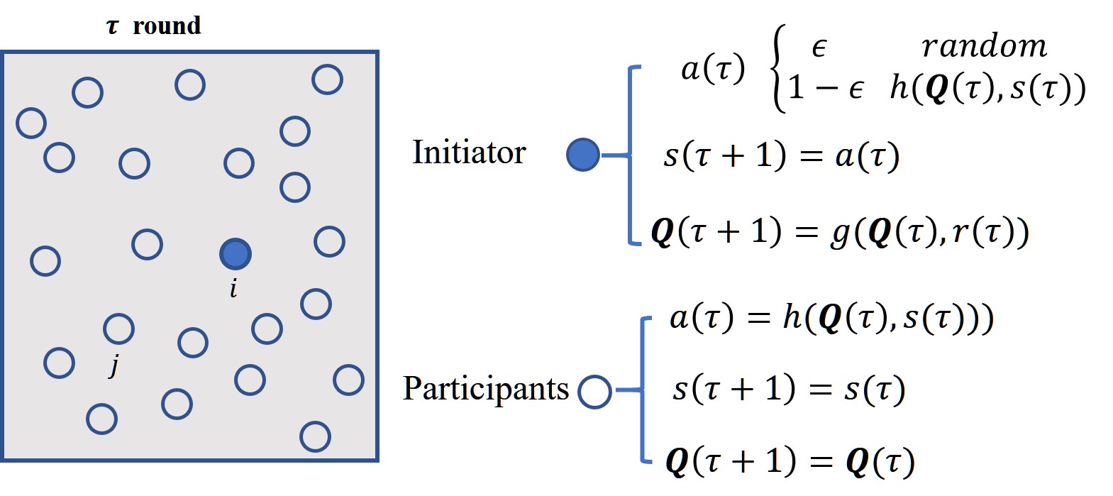
Figure 1: (Color online) The schematic diagram of the updating process in the well-mixed system. At round $\tau$, a game is proposed by an initiator $i$ against all the rest agents known as participants like $j$ in the system. The initiator $i$ takes action according to $h$ function with probability $1-\epsilon$, or acts randomly otherwise. The initiator $i$ both updates its $Q$-table following $g$ function and replaces its state $s$ by current action at the end of round $\tau$, while a participant $j$ only takes action following its Q-table in response, but without updating its Q-table and state.

When the initiator $i$ is in state $s$ at $\tau$th round, it takes action following Q-table

$$a(\tau)=h\left({\bf Q}\left(\tau\right),s(\tau)\right)=\arg\max\limits_{a^{\prime}}\{Q_{sa^{\prime}}(\tau)\},a^{\prime}\in\mathscr{A}$$

with probability $1-\epsilon$, or a random action otherwise. Notice that, $\arg\max\limits_{a^{\prime}}(Q_{sa^{\prime}}(\tau))$ represents the action with the maximal Q-value in the row of state $s$. Each participant in the round always selects the action with the largest value of $Q_{sa^{\prime}}(\tau)$ as Fig.1 shows. At the end of the round, $i$’s state $s(\tau)$ is instead of $s(\tau+1)=a(\tau)$, i.e. $s^{\prime}=a$ in the Eq.(9).

To summarize, the protocol of $Q$-learning algorithm is as follows:

• Initialize matrix $Q$ to zero to mimic the unawareness of agents to the game or environment at beginning, and initialize state $s$ of each agent randomly.

• For each round, a randomly generated initiator $i$ plays the game with the rest agents and chooses the action $a$ with largest value of $Q_{sa^{\prime}}(\tau)$ in the row of current state $s$ with probability $1-\epsilon$, or chooses an action randomly with probability $\epsilon$.

• The $Q_{sa}$ value of the initiator is updated according to Eq. (9), and the state is also updated as $s(\tau+1)=a(\tau)$.

• Each participant only takes the action $a$ with largest value of $Q_{sa^{\prime}}(\tau)$ in the row of its current state $s$ as response, therefore $s(\tau+1)=s(\tau)$.

• Repeat steps 2) – 4) until the system state becomes statistically stable or evolves to the desired time duration.

Notice that agents in RLEGs that adopt reinforcement learning aim to maximize reward gradually rather than birth-death or imitation processes in the traditional evolutionary game and its variants [1, 4, 64]. Besides, the coupling between the environment and agents’ behaviors gives rise to a dynamic environment, which is different from paradigmatic Q-learning algorithm that individuals confront a static environment. This work is also different from the previously studied minority game system [65] that takes into account a periodic environment. Our setting then offers a scenario for complex coevolution where the adaption process and environment influence each other and trigger the emergence of some interesting collective behaviors. In the following, we will show the main results and the impact of various parameters on the actions and dynamical behaviors in the population.

2.2 Simulation Results in $2\times 2$ RLEGs

In the RLEGs for a $2\times 2$ game setting, the actions set and states set are the same as $\mathscr{A}=\mathscr{S}=\{C,D\}$, and the standard payoff matrix $\Pi=(\Pi_{cc},\Pi_{cd};\Pi_{dc},\Pi_{dd})=(6,b;6+b,2)$ with a tunable game parameter $b$. Different ranges of $b$ correspond to different game categories: 1) $b\in[0,2]$ for Prisoner’s Dilemma (PD) with a strict pure Nash equilibrium; 2) $[2,6]$ for Snowdrift (SD) with a weak mixed Nash equilibrium; 3) $(-\infty,0)$ for Stag Hunt (SH) with two strict pure Nash equilibriums and a weak mixed Nash equilibrium; and 4) $(6,\infty)$ for mixed stable (MS) with a mixed weak Nash equilibrium  [1]. The Q-table here is denoted as ${\bf Q}(\tau)=(Q_{cc}(\tau),Q_{cd}(\tau);Q_{dc}(\tau),Q_{dd}(\tau))$ at round $\tau$.

Before going any further, let’s first review the traditional EGs for this $2\times 2$ game, and specifically focus on the stable cooperation preference $f_{c}^{*}$ in the mean-field treatment by replicator dynamics equation (RDE) [1] of EGs. Denoting $\Delta\Pi_{:d}=\Pi_{dd}-\Pi_{cd}$ and $\Delta\Pi_{:c}=\Pi_{cc}-\Pi_{dc}$, in case I), when $\Delta\Pi_{:c}\cdot\Delta\Pi_{:d}<0$, $f_{c}=1$ is the stable fixed point if $\Delta\Pi_{:d}>0$ (PD), and $f_{c}=0$ is stable otherwise. In case II), when $\Delta\Pi_{:c}\cdot\Delta\Pi_{:d}>0$, there is a stable mixed fixed point $f_{c}=\Delta\Pi_{:d}/(\Delta\Pi_{:d}+\Pi_{:c})$ if $\Delta\Pi_{:c}<0$ (SD or MS), otherwise, the fixed-point is unstable (SH). For the latter, cooperation dominates if the initial preference is greater than the point, otherwise, defection dominates. In case II), cooperators’ and defectors’ rewards are identical at the mixed fixed-point.

We first investigate the cooperation prevalence in our RLEGs, as a function of $b$. Here we employ the fraction

$$\rho_{c}(t)=\sum_{l=1}^{N}\delta(a(\tau_{t}^{l})-C)/N$$ (10)

to assess the cooperation preference in the $t$th Monte Carlo (MC) step, which includes $N$ rounds of games denotes as $\tau_{t}^{1},\tau_{t}^{2},\cdots,\tau_{t}^{N}$. When $\delta=1$ if the initiator’s action is $C$ at $\tau_{t}^{l}$ round, and $\delta=0$ otherwise. With these, the average preference over MC step $\langle\rho_{c}\rangle$, is used to measures the cooperation preference.

Figure 2: (Color online) The cooperation preference $\langle\rho_{c}\rangle$ in RLEGs as a function of $b$ under various combination of parameters. The cooperation level for traditional EG $f_{c}^{*}$ is also shown for comparison. The shared parameters in each panel are as follows: a) $\gamma=0.9$, $\epsilon=0.02$ and $N=10000$; b) $\alpha=0.9$, $\epsilon=0.02$ and $N=10000$; c) $\alpha=0.9$, $\gamma=0.9$ and $N=10000$; d) $\alpha=0.9$, $\gamma=0.9$ and $\epsilon=0.02$. The data is averaged over $n_{t}=50000$ runs.

Fig. 2 shows the cooperation preference both in RLEGs by simulations and in EGs as a function of $b$ for a couple of control parameters. A striking result is that, in almost all cases $\langle\rho_{c}\rangle$ are close to $f_{c}^{*}$, which means the cooperation level is equally well when played by AI and by traditional approaches. And this equivalent performance applies to the whole range of parameters, implying the robustness to specific type of games and parameters.

However, a close lookup shows that $\langle\rho_{c}\rangle$ is slightly greater than $f_{c}^{*}$, and the difference $\langle\rho_{c}\rangle-f_{c}^{*}$ depends not only on learning parameters, but also on the game category (i.e. different $b$). In SH and PD region, the gap is time-dependent and enlarged with increasing exploration rate $\epsilon$, but is narrowed down when the system approaches into the MS category. Similar to the dependence of $f_{c}^{*}$ on initialization in SH EGs, $\langle\rho_{c}\rangle$ in SH RLEGs also rely on agents’ initial Q-table and cooperation preferences (Fig. S6 in S2.2). Fig. 2(a-c) show also that the gap is not only sensitive to $\epsilon$ but also to $\alpha$ and $\gamma$ when $b$ is in the SD region.

Figure 3: (Color online) The oscillatory evolution of $\rho_{c}(t)$ under different parameter combinations in RLEGs. The cooperation level for traditional EG $f_{c}^{*}$ is also shown for reference. The parameters are indicated in each panels

To understand these differences, we investigate the time series $\rho_{c}(t)$ for typical cases and we mainly focus on SD games since their differences are most significant. Shown in Fig. 3 explains how the difference between $\langle\rho_{c}\rangle$ and $f_{c}^{*}$ comes from. Unexpectedly, Fig. 3 reveals an oscillatory structure of $\rho_{c}(t)$ when the games are played by AI agents. In a typical period, the cooperation preference increases rapidly after a quiescent stage near $f_{c}^{*}$ and relaxes to $f_{c}^{*}$ afterwards. This explains why the cooperation level is enhanced at almost all cases in RLEGs than in the EGs. Further research shows that the period $T$ and amplitude $A$ of the oscillation increase with $\gamma$ (b), but decrease with $\alpha$ (a), while larger $\epsilon$ increases the amplitude $A$ but reduces the period $T$ (c). The oscillation is covered by the noise in the extreme case $\gamma=0$ that all agents are short-sighted as (d) shows. At last, we discover the oscillatory structure fades away as $b$ approaches $b^{\prime}$ (Fig. S5 in S2.1). It implies that the $b^{\prime}$ is the transition point between oscillation and non-oscillation for the cooperation preference. We would like to note that in the traditional $2\times 2$ EGs, the cooperation preference is always in equilibrium, oscillation is only possible when more than 2 states/actions are available in the system.

Next, we further study the impact of the feature of payoff matrix $\Pi$ on the oscillation dynamics. The above considers the weak Nash equilibrium cases, where is $\Delta\Pi_{:d}/(\Delta\Pi_{:d}+\Pi_{:c})$, is always smaller than $1/2$ in the standard game setting. Here we modify the payoff matrix in SD RLEGs and show that the form of the oscillation is dramatically changed compared to the scenarios shown in Fig. 3 when $\Delta\Pi_{:d}/(\Delta\Pi_{:d}+\Pi_{:c})>1/2$ , see Fig. 4(a). In addition, the oscillation fades away as $\Delta\Pi_{:d}/(\Delta\Pi_{:d}+\Pi_{:c})$ tend to $1/2$ as shown in Fig. 4(b). These suggest that $\Delta\Pi_{:d}/(\Delta\Pi_{:d}+\Pi_{:c})=1/2$ is the threshold separating oscillation form in the SD RLEGs. In Fig. 4(c-d), we also provide typical time series $\rho_{c}(t)$ for PD and MS RLEGs. In both case, the cooperation preference $\rho_{c}$ decay with $t$ to the stable level in the end, without any oscillation expected. These complexities revealed here are absent in the traditional SD EGs, and are unique in multi-agent AI systems.

Figure 4: (Color online) The time series of $\rho_{c}$ in RLEGs for different payoff structures. In (a) and (b), the payoff matrices in SD RLEGs are $\Pi=(6,5;7,2)$ and $(6,3;7,2)$, respectively. (c) shows the time series in a PD RLEG with $b=1.5$ in a standard payoff matrix to reach the stable value $\rho_{c}^{*}=\epsilon/2$ . (d) shows the time series in an MS RLEG with the payoff matrix $(0,3;5,2)$. The learning parameters $\alpha=\gamma=0.9$, $\epsilon=0.02$ and $N=10000$.

3 The analysis

3.1 The analysis of the evolution in a static environment

To understand these observations, we build a system that consists of a number of noninteracting individuals, whose action and state sets $\mathscr{A}\!=\!\mathscr{S}\!=\!\{C,D\}$. Different from RLEGs, rewards for actions $C$ and $D$ are constant and denoted as $r_{c}$ and $r_{d}$ respectively, i.e. the environment is assumed to be static for all individuals. As in RLEG, each individual maximizes reward via reinforcement learning: updates both its Q-table and state. The updating of Q-table in the Q-learning algorithm involves the self-coupling (memory effect), inter-elements coupling (effect of estimated future reward), and environmental coupling (effect of current reward), through the learning parameters $\alpha$, $\gamma$ and the reward of actions.

To update actions, each individual either follows $h$ function with probability $1-\epsilon$ or acts randomly with $\epsilon$. Since the random scheme shares half chance with identical actions of following $h$ function, the individual’s action updating can then be summarized as in Fig. 5(a) and (b). Fig. 5(a) shows update hops between elements in the individual’s Q-table if the action is in line with the results following the $h$ function. In contrast, hops in the cases caused by exploration events is shown in Fig. 5(b). The events in Fig. (a) and (b) could be called as “ freezing events”(f-events) and “melting events”(m-events), respectively. Because $\epsilon/2\ll 1$ is in the model, m-events can be regarded as perturbations in the world of f-events.

If the system follows only f-events, each individual’s Q-table will be “frozen” in such a static environment finally. The freezing rate depends on learning rate $\alpha$ and discounting factor $\gamma$, where a larger $\alpha$ facilitates the freezing process, but $\gamma$ does the opposite (S1.2). When get frozen, the individuals’ behaviors will be in one of three modes as depicted in Fig. 5(c):

• frozen cooperation in the form of C-C mode (CCM) when $\arg\max\limits_{a^{\prime}}\{Q_{sa^{\prime}}\}=C$ for $s=C$;

• frozen defection in the form of D-D mode (DDM) when $\arg\max\limits_{a^{\prime}}\{Q_{sa^{\prime}}\}=D$ for $s=D$;

• cyclic frozen mode in the form of cyclic C-D mode (CDM) when $\arg\max\limits_{a^{\prime}}\{Q_{sa^{\prime}}\}=D$ for $s=C$, and $\arg\max\limits_{a^{\prime}}\{Q_{sa^{\prime}}\}=C$ for $s=D$.

These frozen modes are reminiscent of various attractors in nonlinear dynamics, just the convergence rate towards these attractors is determined by the learning parameters $\alpha$, $\gamma$ and rewards of actions (S1.2), rather than the parameters in equations.

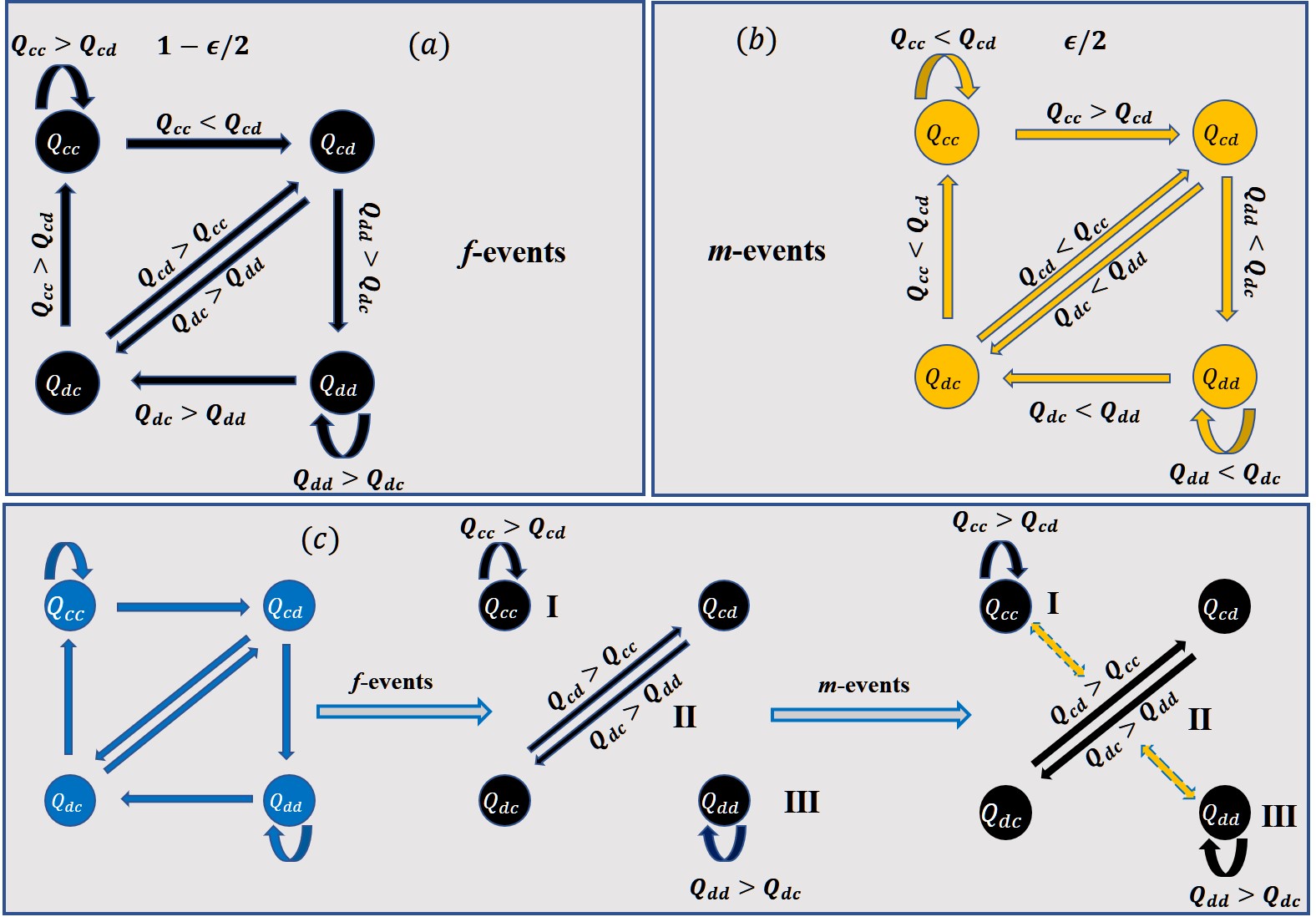
Figure 5: (Color online) The evolution scheme of Q-table in a static environment. (a) and (b) show the hops between elements in Q-table under f-events and m-events, respectively. The conditions of different hops are indicated. (c) shows the freezing and melting processes of behavioral modes under f-events and m-events, respectively. The individual’s behavior will be frozen in one of the three modes (CCM, CDM and DDM) under f-events. But these modes could be potentially melted and interchangeable by m-events.

However, when m-events are present, they do not only perturb individual’s actions but may also “melt” modes as Fig. 5(c) shows. Here, the mode is stable if it is robust to m-events that cannot be melted. According to the analysis, we find that only DDM is stable in a static environment as $r_{c}<r_{d}$ (S1.3), and there is a mode flow CCM $\rightarrow$ CDM $\rightarrow$ DDM if $r_{c}<r_{d}$ and $\epsilon\rightarrow 0$, i.e. the optimal action is reachable through the reinforcement learning in a static environment. The dependence of melting rate of the two unstable modes (i.e., CCM and CDM) on $\epsilon$, $\gamma$, the reward gap $\Delta r=|r_{c}-r_{d}|$, and $\alpha$ shows that the former three factors accelerate the melting process, while $\gamma$ decreases the process (see S1.3). At last, elements of individuals’ Q-table in various modes tend to be identical as $r_{c}=r_{d}$.

Intuitively, Q-table are beliefs aiming for the optimal action for individuals in different states and these beliefs are updated gradually in the evolution. Low learning rate means a strong memory effect for individuals because the old Q-table accounts for history takes a large fraction in the updating. As a result, a large $\alpha$ slows down both the freezing and melting processes. However, short-sighted individuals pay much attention to the reward in current round rather than in future, which means these individuals are more sensitive to the reward gap in the exploratory trials. Meanwhile, the probability of trials is positive to the exploration rate $\epsilon$, therefore, $\gamma$, $\epsilon$ and $\Delta r$ accelerate the melting process. Furthermore, a great difference between elements in the row of state $s$ signifies that it takes longer time to change its belief, i.e. the robustness of the beliefs are enslaved to the gaps between elements in the rows.

3.2 The stability of the $2\times 2$ RLEGs

In a well-mixed RLEG, the reward for a cooperative or defective initiator at round $\tau$ and $r_{c}(\tau)=p_{c}(\tau)\Delta\Pi_{c:}+\Pi_{cd}$ and $r_{d}(\tau)=-p_{c}(\tau)\Delta\Pi_{d:}+\Pi_{dd}$ as $N\rightarrow\infty$, respectively. Here, $\Delta\Pi_{c:}=\Pi_{cc}-\Pi_{cd}$ and $\Delta\Pi_{d:}=\Pi_{dd}-\Pi_{dc}$, and ${\bf p}(\tau)=\{p_{c},p_{d}\}$ denotes the shares of cooperators and defectors in the agents following $h$ function, acting as the environment for current initiator. The process to explore the maximal reward is to narrow reward difference between agents in the evolution. Here, we denote the equilibrium as ${\bf p}^{*}=\{p_{c}^{*},p_{d}^{*}\}$, at which the agent is unable to explore a better mode than the current one, therefore is where the evolution of ${\bf p}$ ideally settles down. Analogy to the Nash equilibrium point in $2\times 2$ game, our equilibrium ${\bf p}^{*}$ can also be classified into two categories: 1) pure and strict, and 2) mixed and weak. For the former, reward for initiators under $f$-events is greater than under $m$-events and $p_{c}^{*}\in\{0,1\}$, while for the latter, reward for initiators in $f$-events equal to in $m$-events, i.e. $r_{c}^{*}=r_{d}^{*}$ at $p_{c}^{*}=\Delta\Pi_{:d}/(\Delta\Pi_{:d}+\Pi_{:c})\in(0,1)$.

However, an equilibrium point ${\bf p}^{*}$ is stable in a RLEG only if the system is able to resist various fluctuations around ${\bf p}^{*}$. For the strict case, initiators are unable to be better off by updating their mode at ${\bf p}^{*}$, such as DDM in PD RLEGs, therefore ${\bf p}^{*}$ is stable. Notice that each pure equilibrium point is stable in $2\times 2$ RLEGs, e.g. $p_{c}^{*}=1$ and $p_{c}^{*}=0$ in the RLEGs for SH setting (Fig. S7 and S2.2).

For the mixed case, based on the payoff matrix $\Pi$, the standard game settings are further divided into three classes:

• $\Delta\Pi_{c:}<0$ and $\Delta\Pi_{d:}<0$ (MS);

• $\Delta\Pi_{c:}>0$ and $\Delta\Pi_{d:}>0$ (SH);

• $\Delta\Pi_{c:}>0$ and $\Delta\Pi_{d:}<0$ (SD).

The results in the static environment show that the gap between elements in each row decreases with time if reward for initiators as cooperator and defector is identical. Thus, agents’ beliefs become fragile gradually to fluctuations regarding ${\bf p}^{*}$, in which $r_{c}^{*}=r_{d}^{*}$. The stability of ${\bf p}^{*}$ rest with feedback from the change of initiators’ belief to various fluctuations, $\delta p_{c}(\tau)=p_{c}(\tau)-p_{c}^{*}\rightarrow 0$.

For class i), since $r_{c}$ ($r_{d}$) decreases (increases) with $p_{c}$, a fluctuation with $\delta p_{c}(\tau)<0$ cause $r_{c}(\tau)>r_{c}^{*}$ ($r_{d}(\tau)<r_{d}^{*}$). The reward change strengthen the beliefs to cooperation but weaken to defection in any events. With the change of the latter belief, $p_{c}$ is increased due to the flux from defectors to cooperators. For a fluctuations with $\delta p_{c}(\tau)>0$, the environment favors defectors rather than cooperators because $r_{c}(\tau)<r_{c}^{*}$ ($r_{d}(\tau)>r_{d}^{*}$) in the fluctuation. Hence, $p_{c}$ would decrease in this case. In short, the equilibrium point ${\bf p}^{*}$ is stable in the MS RLEGs because $\delta p_{c}\cdot dp_{c}/dt<0$ (Fig.4(c)). By contrast, in case ii) ${\bf p}^{*}$ is unstable (see Fig. S6 and S2.2) because the feedback of agent to fluctuations regarding ${\bf p}^{*}$ in the RLEG is just opposite to class i).

In case iii), a standard SD RLEG, both $r_{c}$ and $r_{d}$ increase with $p_{c}$ but the rate of change for $r_{d}$ is higher than for $r_{c}$. Thus, as $\delta p_{c}(\tau)<0$, the beliefs to defection are more fragile than to cooperation in f-events since $r_{d}(\tau)<r_{c}(\tau)<r_{c}^{*}=r_{d}^{*}$ under the fluctuation. Besides, the shares at equilibrium point meet $p_{c}^{*}<p_{d}^{*}$. For these, the flux from defectors to cooperators is higher than the opposite, which results in the increase of $p_{c}$. Therefore, the system is able to resist the fluctuations and keep the system around $p_{c}^{*}$ (Fig. 3). For $\delta p_{c}(\tau)>0$, the rewards for cooperation and defection are $r_{d}(\tau)>r_{c}^{*}$ and $r_{c}(\tau)>r_{d}^{*}$ but $r_{c}(\tau)<r_{d}(\tau)$. So, the beliefs to defection are more fragile than to defection in m-events. Yet, the flux from defectors to cooperators is still higher than the opposite potentially because $p_{c}^{*}<p_{d}^{*}$. The flux will give rise to further increase of $p_{c}$. Hence, the system is unstable for this type of fluctuation. Furthermore, the increase of $\delta p_{c}$ will cause further destruction of agents’ beliefs in m-events. Therefore, an explosive increase of $p_{c}$ is triggered by the cascading effects as Fig.3 (a-c) shows. The qualitative investigation also indicate the oscillation fades away with the gap $p_{d}^{*}-p_{c}^{*}$ (Fig.2, 4 (b) and Fig. S6). Moreover, irrhythmic oscillations in non-standard SD RLEGs replace periodic oscillation in standard SD RLEGs if $p_{c}^{*}>p_{d}^{*}$ (Fig. 4 (a) and Fig. S6).

In fact, during the quiescent stage in standard SD RLEGs, $p_{c}=p_{c}^{*}$, agents’ beliefs are weakened gradually. However, the fluctuations $\delta p_{c}>0$ cause the reward for both actions in the current round is higher than in the past. Therefore, some agents beliefs will be replaced by the new one in m-events, which triggers the increase of cooperators. Thereby, $\epsilon$ improve rate of increase for $\rho_{c}$ during the explosive stage (Fig. 3(c)). In addition, the new belief is strengthened gradually by f-events due to memory effect at quiescent stage although $r_{c}<r_{d}$ at current stage. Yet, the belief for some cooperators will be melted finally because $r_{c}$ is always lower than $r_{d}$ before $p_{c}$ returns to $p_{c}^{*}$. Short memory effect and short-sighted means the reward gap takes a greater effect on the freezing as well as melting process as mentioned before. Therefore, high $\alpha$ and low $\gamma$ decrease the period $T$ as well as the amplitude $A$ (Fig. 3(a-b)). A higher exploration rate is able to cause a sharply explosive increase of $p_{c}$ but also shorten the melting process. Thus, $\epsilon$ takes a more complex effects to $T$ and $A$ in the oscillation as Fig. 3(c) shows.

3.3 The mean-field analysis of PD RLEGs

Here we attempt to construct a mathematical framework on the PD RLEG for the mean-field treatment, since there is a single pure strict equilibrium point for the PD game setting. In the standard PD game setting, an arbitrary initiator’s reward is $r_{d}(\tau)=\bar{\Pi}_{d}(\tau)=(4+b)p_{c}(\tau)+2$ and $r_{c}(\tau)=\bar{\Pi}_{c}(\tau)=(6-b)p_{c}(\tau)+b$ as a defector and cooperator, respectively. Here, $r_{d}$ is alway higher than $r_{c}$ due to $p_{c}(\tau)\in[0,1]$. Therefore, the cooperation preference of initiators decreases in exploration trials. And, the preference is the same for initiators and participants just switch their roles in different rounds. This leads to self-consistent results in the end that $p_{c}(\infty)=p_{c}^{*}=0$ and $\langle\rho_{c}\rangle=\epsilon/2$ because $\langle\rho_{c}\rangle=p_{c}^{*}(1-\epsilon)+\epsilon/2$. It means that $\langle\rho_{c}\rangle$ only depends on the exploration rate $\epsilon$ in the PD RLEGs (Fig. 2).

Figure 6: (Color online) The time evolution of $\bar{{\bf Q}}(t)$ and Q-table $\tilde{\bf Q}^{*}$ at the stable point $p_{c}^{*}$. (a-d) show the $\bar{Q}_{cc}(t)$, $\bar{Q}_{cd}(t)$, $\bar{Q}_{dc}(t)$ and $\bar{Q}_{dd}(t)$, respectively. The time points at which the elements become stable are indicated. The elements in $\tilde{\bf{Q}}^{*}$ are displayed (black lines) for reference. The parameter setting is the same as Fig. 4(a).

Thus, the stable Q-table for all agents are uniform and is

$$\tilde{\bf{Q}}^{*}=\left(\begin{array}[]{cc}\frac{\gamma(2-b)+b}{1-\gamma}&\frac{b}{1-\gamma}\\ \frac{\gamma(2-b)+b}{1-\gamma}&\frac{b}{1-\gamma}\end{array}\right),$$ (13)

since the $r_{c}=b$ and $r_{d}=2$ at $p_{c}^{*}=0$. To check the analysis, we show the time series of the average Q-table $\bar{\bf{Q}}(t)$

$$\bar{\bf{Q}}(t)=\left(\begin{array}[]{cc}\frac{\sum_{k=1}^{N}Q_{cc}^{k}(\tau_{t}^{N})}{N}&\frac{\sum_{k=1}^{N}Q_{cd}^{k}(\tau_{t}^{N})}{N}\\ \frac{\sum_{k=1}^{N}Q_{dc}^{k}(\tau_{t}^{N})}{N}&\frac{\sum_{k=1}^{N}Q_{dd}^{k}(\tau_{t}^{N})}{N}\end{array}\right)$$ (16)

in the Fig. 6. Here, $\tau_{t}^{N}$ is the last round in $t$th MC step and $Q_{sa}^{k}(\tau_{t}^{N})$ denotes the corresponding element of agent $k$’s Q-table at $\tau_{t}^{N}$th round. $\bar{\bf{Q}}(t)$ and $\tilde{\bf{Q}}^{*}$ in Fig. 6 show that the result of stable Q-table is reliable in our analysis. Moreover, another result in the static environment is also reflected in PD RLEGs, that is the convergence rate for the elements in Q-table decreases as $\bar{Q}_{dd}$, $\bar{Q}_{cd}$, $\bar{Q}_{dc}$, and $\bar{Q}_{cc}$. $\tilde{\bf Q}$ manifests one element dominant another one for the rival elements because $\tilde{Q}_{dd}^{*}>\tilde{Q}_{dc}^{*}$ and $\tilde{Q}_{cd}^{*}>\tilde{Q}_{cc}^{*}$.

A mean-field method is employed to calculate ${\bf Q}(t)$ and $\rho_{c}(t)$ numerically as Fig. 4(a) and Fig. 6 shows. In Eq. (32) of mean-field method, we replace each agents’ Q-table with the mean Q-table. Besides, $\rho_{c}(\tau)$ means the fraction of agents at $C$ state in the system, which is slightly different from cases in the simulation.

 

$$\left\{\begin{array}[]{rl}r_{c}(\tau)=&\left[\rho_{c}(\tau)\cdot\Theta(\Delta\bar{Q}_{c:}(\tau))+\rho_{d}(\tau)\cdot\Theta(-\Delta\bar{Q}_{d:}(\tau))\right]\cdot\Pi_{cc}+\\ &\left[\rho_{c}(\tau)\cdot\Theta(-\Delta\bar{Q}_{c:}(\tau))+\rho_{d}(\tau)\cdot\Theta(\Delta\bar{Q}_{d:}(\tau))\right]\cdot\Pi_{cd}\\ r_{d}(\tau)=&\left[\rho_{c}(\tau)\cdot\Theta(\Delta\bar{Q}_{c:}(\tau))+\rho_{d}(\tau)\cdot\Theta(-\Delta\bar{Q}_{d:}(\tau))\right]\cdot\Pi_{dc}+\\ &\left[\rho_{c}(\tau)\cdot\Theta(-\Delta\bar{Q}_{c:}(\tau))+\rho_{d}(\tau)\cdot\Theta(\Delta\bar{Q}_{d:}(\tau))\right]\cdot\Pi_{dd}\\ \rho_{c}(\tau+1)=&\left\{\rho_{c}(\tau)\cdot\left[\frac{\epsilon}{2}+\left(1-\epsilon)\cdot\Theta(\Delta\bar{Q}_{c:}(\tau)\right)\right]+\rho_{d}(\tau)\cdot\left[\frac{\epsilon}{2}+\left(1-\epsilon)\cdot\Theta(\Delta\bar{Q}_{d:}(\tau)\right)\right]\right\}\cdot\rho_{c}(\tau)\\ &+\rho_{c}(\tau)\cdot\left[\frac{\epsilon}{2}+(1-\epsilon)\cdot\Theta(-\Delta\bar{Q}_{c:}(\tau))\right]\frac{N\cdot\rho_{c}(\tau)-1}{N}\\ &+\rho_{d}(\tau)\cdot\left[\frac{\epsilon}{2}+(1-\epsilon)\cdot\Theta(-\Delta\bar{Q}_{d:}(\tau))\right]\frac{N\cdot\rho_{c}(\tau)+1}{N}\\ \bar{Q}_{cc}(\tau+1)=&\rho_{c}(\tau)\cdot\left[\frac{\epsilon}{2}+(1-\epsilon)\cdot\Theta(\Delta\bar{Q}_{c:}(\tau))\right]\cdot\left[\frac{(N-1)\cdot\bar{Q}_{cc}(\tau)+(1-\alpha)\cdot\bar{Q}_{cc}(\tau)+\alpha\cdot(\gamma\cdot\bar{Q}^{\max}_{ca^{\prime}}(\tau)+r_{c}(\tau))}{N}\right]\\ &+\left\{1-\rho_{c}(\tau)\cdot\left[\frac{\epsilon}{2}+(1-\epsilon)\cdot\Theta(\Delta\bar{Q}_{c:}(\tau))\right]\right\}\cdot\bar{Q}_{cc}(\tau)\\ \bar{Q}_{dd}(\tau+1)=&\rho_{d}(\tau)\cdot\left[\frac{\epsilon}{2}+(1-\epsilon)\cdot\Theta(\Delta\bar{Q}_{d:}(\tau))\right]\cdot\left[\frac{(N-1)\cdot\bar{Q}_{dd}(\tau)+(1-\alpha)\cdot\bar{Q}_{dd}(\tau)+\alpha\cdot(\gamma\cdot{Q}^{\max}_{da^{\prime}}(\tau)+r_{d}(\tau))}{N}\right]\\ &+\left\{1-\rho_{d}(\tau)\cdot\left[\frac{\epsilon}{2}+(1-\epsilon)\cdot\Theta(\Delta\bar{Q}_{d:}(\tau))\right]\right\}\cdot\bar{Q}_{dd}(\tau)\\ \bar{Q}_{cd}(\tau+1)=&\rho_{c}(\tau)\cdot\left[\frac{\epsilon}{2}+(1-\epsilon)\cdot\Theta(-\Delta\bar{Q}_{c:}(\tau))\right]\cdot\left[\frac{(N-1)\cdot\bar{Q}_{cd}(\tau)+(1-\alpha)\cdot\bar{Q}_{cd}(\tau)+\alpha\cdot(\gamma\cdot\bar{Q}^{\max}_{da^{\prime}}(\tau)+r_{d}(\tau))}{N}\right]\\ &+\left\{1-\rho_{c}(\tau)\cdot\left[\frac{\epsilon}{2}+(1-\epsilon)\cdot\Theta(-\Delta\bar{Q}_{c:}(\tau))\right]\right\}\cdot\bar{Q}_{cd}(\tau)\\ \bar{Q}_{dc}(\tau+1)=&\rho_{d}(\tau)\cdot\left[\frac{\epsilon}{2}+(1-\epsilon)\cdot\Theta(-\Delta\bar{Q}_{d:}(\tau))\right]\cdot\left[\frac{(N-1)\cdot\bar{Q}_{dc}(\tau)+(1-\alpha)\cdot\bar{Q}_{dc}(\tau)+\alpha\cdot(\gamma\cdot\bar{Q}^{\max}_{ca^{\prime}}(\tau)+r_{c}(\tau))}{N}\right]\\ &+\left\{1-\rho_{c}(\tau)\cdot\left[\frac{\epsilon}{2}+(1-\epsilon)\cdot\Theta(-\Delta\bar{Q}_{d:}(\tau))\right]\right\}\cdot\bar{Q}_{dc}(\tau)\end{array}\right.$$ (32)

Here, $\Theta(\cdots)$ is the Heaviside function

$$\Theta(x)=\left\{\begin{array}[]{l}1,\quad x>0,\\ 1/2,\quad x=0,\\ 0,\quad x<0\end{array}\right.$$ (36)

and $\Delta\bar{Q}_{c:}(\tau)=\bar{Q}_{cc}(\tau)-\bar{Q}_{cd}(\tau)$, $\Delta\bar{Q}_{d:}=\bar{Q}_{dd}(\tau)-\bar{Q}_{dc}(\tau)$.                                                                                                                                     

The final cooperation preference, $\bar{\bf Q}$ and the ranking of convergence rates in the calculation are identical to the simulation results. However, the times series are different during the transient process. The results imply that, on one hand, the mean-field method successfully captures long-term dynamics in the PD RLEGs since all agents’ Q-table are identical in the end; on the other hand, the heterogeneity of Q-table for different agents cannot be omitted during transient process and will cause deviations as shown. The numerical results of MS and SD RLEGs also indicate that the mean-field results is decent only if heterogeneity of agents’ Q-table is negligible during whole process ( Fig. S8 and Fig. S9 in S2.2).

3.4 Oscillation in the RLEGs for Rock-Paper-Scissors game

Different from low-degree of freedom of fluctuation for the $2\times 2$ games setting, we pay attention to the game setting with high-degree of freedom of fluctuation at the equilibrium point, ${\bf p}^{*}$. Here, the RLEGs for rock-paper-scissors (RPS) game is investigated by simulations. In the corresponding RLEGs, the action and state sets are $\mathscr{A}\!=\!\mathscr{S}\!=\!\{R,P,S\}$, and the payoff matrix is

$$\Pi=\left(\begin{array}[]{ccc}\Pi_{rr}&\Pi_{rp}&\Pi_{rs}\\ \Pi_{pr}&\Pi_{pp}&\Pi_{ps}\\ \Pi_{sr}&\Pi_{sp}&\Pi_{ss}\end{array}\right)=\left(\begin{array}[]{ccc}0&-b_{1}&1\\ 1&0&-b_{1}\\ -b_{1}&1&0\end{array}\right)$$ (43)

with a tunable parameter $b_{1}$. In the traditional EGs, the evolution of collective behaviors is described by ${\bf f}=\{f_{a_{\underline{i}}},a_{\underline{i}}\in\mathscr{A}\}$ in a three-dimensional simplex. Here, $f_{a_{\underline{i}}}$ is the action preference of $a_{\underline{i}}$. The mean field treatment [1] by the RDE of traditional EGs reveals that: 1) the fixed point ${\bf f^{*}}=\{1/3,1/3,1/3\}$ is globally stable in the case of $b_{1}<1$; 2) the fixed point is unstable if $b_{1}>1$; 3) there is a center surrounded by neutral oscillation for $b_{1}=1$. Here, we point out that in the case 2) the trajectories of the replicator dynamics starting from arbitrary interior initial conditions will converge to the boundary of the simplex in oscillations with the increasing amplitude.

Figure 7 shows the time series of the fraction of the three species in the initiators

$$\rho_{a_{\underline{i}}}(t)=\frac{\sum_{i=1}^{N}\delta(a(\tau_{t}^{k})-a_{\underline{i}})}{N},\forall a_{\underline{i}}\in{\mathscr{A}}.$$ (44)

And the shown with red dots are $1/3\pm\Delta{\bm{\rho}}$, where $\Delta{\bm{\rho}}$ is the deviation that is computed as the Euclidean distance between ${\bm{\rho}}(t)$ and ${\bm{\rho}}^{*}$, in which ${\bm{\rho}}=\{\rho_{a_{\underline{i}}}|a_{\underline{i}}\in\mathscr{A}\}$ and ${\bm{\rho}}^{*}=\{1/3,1/3,1/3\}$. Fig. 7(a) shows the case for $b_{1}<1$ where ${\bm{\rho}}^{*}$ is globally stable at large except for some small irregular bursts. However, in the case of $b_{1}\geq 1$ as shown in Fig. 7(b, c), clear oscillatory structures emerge in the time series in the RPS RLEGs. The difference for (b) and (c) lies in the envelope of these oscillatory trajectories, where in the case of $b_{1}=1$ there is some moments that the amplitude of oscillation almost diminishes while the oscillation is always significant in the case of $b_{1}>1$.

In the RLEGs for the RPS game, the equilibrium point for shares ${\bf p}^{*}=\{1/3,1/3,1/3\}$, which is mixed and weak. The previous analysis shows that the initiators exploring the optimal mode leads ${\bf p}$ toward to ${\bf p}^{*}$ and reduce the reward gap between actions gradually. During the exploring process, the amplitude of the oscillation is diminished. However, the agent’s belief becomes fragile to fluctuations since the gaps between elements in state row of Q-table are reduced. ${\bf p}^{*}$ is stable if the system is able to resist various fluctuations. The simulation shows that the decrease of $b_{1}$ makes the system less sensitive to the fluctuations (a-c) as in EGs. Compare to the EGs, the stability of ${\bf p}^{*}$ depends more on properties of payoff matrix in RLEGs, they cause abundant collective behaviors in the RLEGs for the identical RPS game setting. Furthermore, the trajectories here are different from the cases in the SD RLEGs because the system needs to resist more comlex and diverse fluctuations to keep ${\bf p}$ stay around ${\bf p}^{*}$.

Figure 7: (Color online) The time series of the three fractions in the RPS RLEGs. The parameter in (a-c) $b_{1}=0.7,1$ and $2$, respectively. The red dots in the figure is $1/3\pm\Delta{\bm{\rho}}(t)$. The learning parameters are $\alpha=\gamma=0.9$ and $\epsilon=0.02$, with the system size being $N=10000$.

4 Discussion and Conclusion

In this work, we propose a reinforcement learning evolutionary game model for a general two-player multi-actions ($2\times n_{a}$) game setting, where agents improve their adaption through Q-learning algorithm rather than birth-death process or imitation in the traditional evolutionary games. A striking finding is that the resulting cooperation preference in RLEGs is the same as the traditional EGs in $2\times 2$ cases, resting on the Nash Equilibrium of the games. Furthermore we show that Snowdrift game cases present an oscillatory evolution with explosive cooperation in between, exhibiting quite different dynamical mechanism from the traditional EGs.

We investigate dynamics of an analogous individual’s Q-table as well as its behavior in a static environment in theory, and apply these to analyze the stability of the RLEGs for the standard $2\times 2$ game setting. The analysis indicates that the pure and strict equilibrium point is stable in the RLEGs for the game. Different from the stable mixed and weak equilibrium point for the MS region, oscillatory dynamics potentially emerges for the SD region. The qualitative analysis explicitly shows the impact of learning parameters on the oscillatory dynamics in the SD RLEGs: 1) Low learning rate and long-term sight is beneficial to amplitude and period by the increasing cascading effects after the breakdown of stability; 2) The long-sighted agents prolong the delay time to explore optimal action, the quiescent stage, and amplify the amplitude; 3) Higher exploration rate signifies a sharper increase of cooperation preference after the quiescent stage. Therefore, low learning rate and high discount factor as well as exploration rate facilitate the emergence of oscillation in the RLEGs.

Based on these analysis, one learns that a variety of collective behavior results from the dependence of stability at the equilibrium point for shares in RLEGs on more properties of the payoff matrix than in EGs. Furthermore, a numerical method combining with mean-field is put forward to obtain the dynamics of cooperation preference and average Q-table in the PD game. The result is partly consistent with the simulation, especially the final preference and average Q-table, and analysis in the static environment. We also show that the oscillatory dynamics is general in the RLEGs when with a mixed and weak equilibrium point for shares, such as Rock-Paper-Scissors game, where the collective behavior is also quite different from the corresponding traditional EGs.

Our work could lay out a foundation for further systematic investigation of evolutionary games from the perspective of machine learning. First, the simulations and analysis in the static environment contribute to the further understanding analytically in the future. Moreover, the numerical method embedding the mean-field takes the first step to build a mathematical framework of the RLEGs. At last, our work may also aid to understand the explosive events and oscillating behaviors in the society since reinforcement learning actually mimics the introspectiveness in human behavior patterns.

References

- [1] Martin A Nowak. Evolutionary dynamics. Harvard University Press, 2006.
- [2] Alexander J Stewart and Joshua B Plotkin. Extortion and cooperation in the prisoner’s dilemma. Proceedings of the National Academy of Sciences, 109(26):10134–10135, 2012.
- [3] Kristian Moss Bendtsen, Florian Uekermann, and Jan O Haerter. Expert game experiment predicts emergence of trust in professional communication networks. Proceedings of the National Academy of Sciences, 113(43):12099–12104, 2016.
- [4] Stuart A West, Ashleigh S Griffin, and Andy Gardner. Evolutionary explanations for cooperation. Current Biology, 17(16):R661–R672, 2007.
- [5] Andrew FG Bourke. Principles of social evolution. Oxford University Press, 2011.
- [6] William D Hamilton. The genetical evolution of social behaviour. ii. Journal of theoretical biology, 7(1):17–52, 1964.
- [7] R Craig Maclean and C Brandon. Stable public goods cooperation and dynamic social interactions in yeast. Journal of evolutionary biology, 21(6):1836–1843, 2008.
- [8] Duncan Greig and Michael Travisano. The prisoner’s dilemma and polymorphism in yeast suc genes. Proceedings of the Royal Society of London B: Biological Sciences, 271(Suppl 3):S25–S26, 2004.
- [9] J Maynard Smith and George R Price. The logic of animal conflict. Nature, 246(5427):15, 1973.
- [10] Ali R Zomorrodi and Daniel Segrè. Genome-driven evolutionary game theory helps understand the rise of metabolic interdependencies in microbial communities. Nature Communications, 8(1):1563, 2017.
- [11] Jun Tanimoto. Impact of deterministic and stochastic updates on network reciprocity in the prisoner’s dilemma game. Physical Review E, 90(2):022105, 2014.
- [12] John Realpe-Gómez, Giulia Andrighetto, Luis Gustavo Nardin, and Javier Antonio Montoya. Balancing selfishness and norm conformity can explain human behavior in large-scale prisoner’s dilemma games and can poise human groups near criticality. Physical Review E, 97(4):042321, 2018.
- [13] James M Allen, Anne C Skeldon, and Rebecca B Hoyle. Social influence preserves cooperative strategies in the conditional cooperator public goods game on a multiplex network. Physical Review E, 98(6):062305, 2018.
- [14] Björn Lindström and Philippe N Tobler. Incidental ostracism emerges from simple learning mechanisms. Nature Human Behaviour, page 1, 2018.
- [15] Daeyeol Lee. Game theory and neural basis of social decision making. Nature neuroscience, 11(4):404, 2008.
- [16] Alan G Sanfey. Social decision-making: insights from game theory and neuroscience. Science, 318(5850):598–602, 2007.
- [17] Lei Zhou, Bin Wu, Vítor V Vasconcelos, and Long Wang. Simple property of heterogeneous aspiration dynamics: Beyond weak selection. Physical Review E, 98(6):062124, 2018.
- [18] Jianlei Zhang, Chunyan Zhang, Ming Cao, and Franz J Weissing. Crucial role of strategy updating for coexistence of strategies in interaction networks. Physical Review E, 91(4):042101, 2015.
- [19] Matjaž Perc, Jillian J Jordan, David G Rand, Zhen Wang, Stefano Boccaletti, and Attila Szolnoki. Statistical physics of human cooperation. Physics Reports, 687:1–51, 2017.
- [20] Adam Bear and David G Rand. Intuition, deliberation, and the evolution of cooperation. Proceedings of the National Academy of Sciences, 113(4):936–941, 2016.
- [21] Dirk Helbing and Wenjian Yu. The outbreak of cooperation among success-driven individuals under noisy conditions. Proceedings of the National Academy of Sciences, 106(10):3680–3685, 2009.
- [22] Linjie Liu, Xiaojie Chen, and Matjaž Perc. Evolutionary dynamics of cooperation in the public goods game with pool exclusion strategies. Nonlinear Dynamics, pages 1–18, 2019.
- [23] Christian Hilbe, Luis A Martinez-Vaquero, Krishnendu Chatterjee, and Martin A Nowak. Memory-n strategies of direct reciprocity. Proceedings of the National Academy of Sciences, 114(18):4715–4720, 2017.
- [24] Ryo Matsuzawa, Jun Tanimoto, and Eriko Fukuda. Spatial prisoner’s dilemma games with zealous cooperators. Physical Review E, 94(2):022114, 2016.
- [25] Sabin Roman and Markus Brede. Topology-dependent rationality and quantal response equilibria in structured populations. Phys. Rev. E, 95:052310, May 2017.
- [26] David G Rand, Martin A Nowak, James H Fowler, and Nicholas A Christakis. Static network structure can stabilize human cooperation. Proceedings of the National Academy of Sciences, 111(48):17093–17098, 2014.
- [27] Wen-Xu Wang, Jie Ren, Guanrong Chen, and Bing-Hong Wang. Memory-based snowdrift game on networks. Physical Review E, 74(5):056113, 2006.
- [28] Pierre Buesser and Marco Tomassini. Evolution of cooperation on spatially embedded networks. Physical Review E, 86(6):066107, 2012.
- [29] Carlos P Roca, José A Cuesta, and Angel Sánchez. Effect of spatial structure on the evolution of cooperation. Physical Review E, 80(4):046106, 2009.
- [30] W Zhang, YS Li, P Du, C Xu, and PM Hui. Phase transitions in a coevolving snowdrift game with costly rewiring. Physical Review E, 90(5):052819, 2014.
- [31] Zhi-Xi Wu and Zhihai Rong. Boosting cooperation by involving extortion in spatial prisoner’s dilemma games. Physical Review E, 90(6):062102, 2014.
- [32] Rubén J Requejo and Juan Camacho. Coexistence of cooperators and defectors in well mixed populations mediated by limiting resources. Physical review letters, 108(3):038701, 2012.
- [33] Jorge Pena, Henri Volken, Enea Pestelacci, and Marco Tomassini. Conformity hinders the evolution of cooperation on scale-free networks. Physical Review E, 80(1):016110, 2009.
- [34] Ryszard S Michalski, Jaime G Carbonell, and Tom M Mitchell. Machine learning: An artificial intelligence approach. Springer Science & Business Media, 2013.
- [35] Yann LeCun, Yoshua Bengio, and Geoffrey Hinton. Deep learning. nature, 521(7553):436, 2015.
- [36] Jérôme Tubiana and Rémi Monasson. Emergence of compositional representations in restricted boltzmann machines. Physical review letters, 118(13):138301, 2017.
- [37] Richard S Sutton and Andrew G Barto. Reinforcement learning: An introduction. MIT press, 2018.
- [38] Art Lew and Holger Mauch. Dynamic programming: A computational tool, volume 38. Springer, 2006.
- [39] Lucian Busoniu, Robert Babuska, Bart De Schutter, and Damien Ernst. Reinforcement learning and dynamic programming using function approximators. CRC press, 2010.
- [40] Nasser M Nasrabadi. Pattern recognition and machine learning. Journal of electronic imaging, 16(4):049901, 2007.
- [41] Clement Farabet, Camille Couprie, Laurent Najman, and Yann LeCun. Learning hierarchical features for scene labeling. IEEE transactions on pattern analysis and machine intelligence, 35(8):1915–1929, 2013.
- [42] L Shi, XC Wang, and YS Wang. Artificial neural network models for predicting 1-year mortality in elderly patients with intertrochanteric fractures in china. Brazilian Journal of Medical and Biological Research, 46(11):993–999, 2013.
- [43] Byung Ju Kim and Sung Hou Kim. Prediction of inherited genomic susceptibility to 20 common cancer types by a supervised machine-learning method. Proceedings of the National Academy of Sciences of the United States of America, 115(6):201717960, 2018.
- [44] Pooya Mobadersany, Safoora Yousefi, Mohamed Amgad, David A Gutman, Jill S Barnholtz-Sloan, José E Velázquez Vega, Daniel J Brat, and Lee AD Cooper. Predicting cancer outcomes from histology and genomics using convolutional networks. Proceedings of the National Academy of Sciences, page 201717139, 2018.
- [45] Jonathan J Tompson, Arjun Jain, Yann LeCun, and Christoph Bregler. Joint training of a convolutional network and a graphical model for human pose estimation. In Advances in neural information processing systems, pages 1799–1807, 2014.
- [46] Volodymyr Mnih, Koray Kavukcuoglu, David Silver, Andrei A Rusu, Joel Veness, Marc G Bellemare, Alex Graves, Martin Riedmiller, Andreas K Fidjeland, Georg Ostrovski, et al. Human-level control through deep reinforcement learning. Nature, 518(7540):529, 2015.
- [47] Noam Brown and Tuomas Sandholm. Superhuman ai for heads-up no-limit poker: Libratus beats top professionals. Science, 359(6374):418–424, 2018.
- [48] Chaoxu Mu and Ke Wang. Approximate-optimal control algorithm for constrained zero-sum differential games through event-triggering mechanism. Nonlinear Dynamics, 95(4):2639–2657, 2019.
- [49] David C Parkes and Michael P Wellman. Economic reasoning and artificial intelligence. Science, 349(6245):267–272, 2015.
- [50] Ritankar Das and David J Wales. Energy landscapes for a machine-learning prediction of patient discharge. Physical Review E, 93(6):063310, 2016.
- [51] Timnit Gebru, Jonathan Krause, Yilun Wang, Duyun Chen, Jia Deng, Erez Lieberman Aiden, and Li Fei-Fei. Using deep learning and google street view to estimate the demographic makeup of neighborhoods across the united states. Proceedings of the National Academy of Sciences, page 201700035, 2017.
- [52] Behrooz Raeisy, Shapoor Golbahar Haghighi, and Ali Akbar Safavi. Active methods to control periodic acoustic disturbances invoking q-learning techniques. Nonlinear Dynamics, 74(4):1317–1330, 2013.
- [53] David Silver, Thomas Hubert, Julian Schrittwieser, Ioannis Antonoglou, Matthew Lai, Arthur Guez, Marc Lanctot, Laurent Sifre, Dharshan Kumaran, Thore Graepel, et al. A general reinforcement learning algorithm that masters chess, shogi, and go through self-play. Science, 362(6419):1140–1144, 2018.
- [54] A Potapov and MK Ali. Convergence of reinforcement learning algorithms and acceleration of learning. Physical Review E, 67(2):026706, 2003.
- [55] Richard S Sutton. Learning to predict by the methods of temporal differences. Machine learning, 3(1):9–44, 1988.
- [56] Richard E Bellman and Stuart E Dreyfus. Applied dynamic programming, volume 2050. Princeton university press, 2015.
- [57] Arnold Kaufmann. Graphs dynamic programming and finite games. Technical report, 1967.
- [58] Hado Van Hasselt, Arthur Guez, and David Silver. Deep reinforcement learning with double q-learning. In AAAI, volume 2, page 5. Phoenix, AZ, 2016.
- [59] Hado V Hasselt. Double q-learning. In Advances in Neural Information Processing Systems, pages 2613–2621, 2010.
- [60] Francisco S Melo. Convergence of q-learning: A simple proof. Institute Of Systems and Robotics, Tech. Rep, pages 1–4, 2001.
- [61] Christopher JCH Watkins and Peter Dayan. Q-learning. Machine learning, 8(3-4):279–292, 1992.
- [62] Ming Cao, A Stephen Morse, and Brian DO Anderson. Coordination of an asynchronous multi-agent system via averaging. IFAC Proceedings Volumes, 38(1):17–22, 2005.
- [63] Hong-Li Zeng, Mikko Alava, Erik Aurell, John Hertz, and Yasser Roudi. Maximum likelihood reconstruction for ising models with asynchronous updates. Physical review letters, 110(21):210601, 2013.
- [64] Alexander J Stewart and Joshua B Plotkin. Collapse of cooperation in evolving games. Proceedings of the National Academy of Sciences, 111(49):17558–17563, 2014.
- [65] Si-Ping Zhang, Ji-Qiang Zhang, Zi-Gang Huang, Bing-Hui Guo, Zhi-Xi Wu, and Jue Wang. Collective behavior of artificial intelligence population: transition from optimization to game. Nonlinear Dynamics, pages 1–11, 2019.