Stochastic order parameter dynamics for phase coexistence in heat conduction

Abstract

We propose a stochastic order parameter model for describing phase coexistence in steady heat conduction near equilibrium. By analyzing the stochastic dynamics with a non-equilibrium adiabatic boundary condition, where total energy is conserved over time, we derive a variational principle that determines thermodynamic properties in non-equilibrium steady states. The resulting variational principle indicates that the temperature of the interface between the ordered region and the disordered region becomes greater (less) than the equilibrium transition temperature in the linear response regime when the thermal conductivity in the ordered region is less (greater) than that in the disordered region. This means that a super-heated ordered (super-cooled disordered) state appears near the interface, which was predicted by an extended framework of thermodynamics proposed in [N. Nakagawa and S.-i. Sasa, Liquid-gas transitions in steady heat conduction, Phys. Rev. Lett. 119, 260602, (2017).]

I Introduction

Phase coexistence, such as liquid-gas coexistence, is ubiquitous in nature. As the most idealized situation, phase coexistence under equilibrium conditions has been studied. For example, the liquid-gas coexistence temperature is determined by the equality of the chemical potential of liquid and gas at constant pressure. The pressure dependence of the coexistence temperature is related to the latent heat and the volume jump at the transition point, which is known as the Clausius-Clapeyron equation. These are important consequences of thermodynamics Callen .

In addition to equilibrium systems, phase coexistence gives rise to a rich variety of phenomena out of equilibrium such as flow boiling heat transfer, pattern formation in crystal growth, and motility-induced phase separation boiling ; crystal ; Cannell ; Zhong ; Ahlers ; mips . Moreover, as an interesting phenomenon, it has been reported that heat flows from a colder side to a hotter side in a transient regime for continuous heating Urban . One may expect that a deterministic hydrodynamic equation incorporating interface thermodynamics, which is referred to as the Navier-Stokes-Korteweg equation (See Anderson98 for a review), generalized hydrodynamics Bedeaux03 , or dynamical van der Walls theory Onuki , could describe such dynamical phenomena.

However, the situation is not so obvious. Because the macroscopic description is obtained by the coarse-graining of microscopic mechanical systems, the noise inevitably appears. The noise properties are determined by the fluctuation-dissipation relation of the second kind at equilibrium, and the relation is also assumed for systems out of equilibrium. Such a framework is called fluctuating hydrodynamics Schmitz or macroscopic fluctuation theory Bertini-rev . For standard cases such as simple homogeneous fluids, the noise effects are so weak that the thermodynamic behavior is well-approximated by the noiseless limit, while it has been known that noises substantially modify the macroscopic behavior for systems in low-dimensions FNS or near the critical point HH . As another example of such strong noise effects, in this paper, we study phase coexistence in steady heat conduction. For simplicity, we assume that the system is divided into two phases by a macroscopic planer interface across which the heat flows in a simple cuboid geometry, as shown in Fig. 1.

The most impressive phenomenon exhibited by the strong noise effect is that the interface temperature $\theta$ deviates from the equilibrium transition temperature $T_{c}$. That is, a super-heated ordered state or a super-cooled disordered state stably appears locally near the interface. It should be noted that this phenomenon was predicted by an extended framework of thermodynamics for heat conduction systems NS , which we call global thermodynamics NS2 . Remarkably, despite the difference of theoretical frameworks, our result on $\theta-T_{c}$ qualitatively agrees with the prediction of this thermodynamic framework up to a multiplicative numerical constant. The main purpose of this paper is to calculate the interface temperature based on a stochastic model that exhibits the phenomenon. See (VI.40) for the main result.

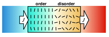
Figure 1: Schematic of setup. The configuration of a single interface is displayed, where the heat flux $J<0$.

I.1 Highlight of the paper

Now, we describe the highlight of the paper.

Model

Among many first-order transitions, we specifically study the order-disorder transition associated with the ${\bf Z}_{2}$ symmetry breaking. This is the simplest case of symmetry breaking, and it is easily generalized to other complicated symmetry breakings, such as the nematic-isotropic transition in liquid crystals, which may be relevant in experiments nematic-isotropic . Although the liquid-gas transition may be most popular in the first-order transition, we study this phenomenon in another paper. See the second paragraph in Sec. VII for related discussions.

For the order-disorder transition associated with the ${\bf Z}_{2}$ symmetry, one may recall a Ginzburg-Landau equation that includes the interface thermodynamics as a gradient term. However, because this model describes the order parameter dynamics with the isothermal condition, it cannot be used for heat conduction systems. We must at least consider a coupled equation of the order parameter density field and the energy density field. When we consider a stochastic model as a generalization of the Ginzburg-Landau model, it is best to use the concept of the Onsager theory as follows. First, we specify a set of dynamical variables. Then, under the assumption of local thermodynamics, we consider the minimum form of dissipation and noise with the detailed balance condition at equilibrium. In Sec. II, following these concepts, we present deterministic and stochastic order parameter dynamics. See (II.65), (II.66), and (II.67) for the final form of stochastic dynamics. We next describe an interface between the ordered region and the disordered region within a framework of the deterministic dynamics in Sec. III. We then discuss how fluctuations of the interface position play an inevitable role in thermodynamic behavior.

Theoretical method

The theory for stochastic models related to thermodynamics has developed significantly over the last two decades Sekimoto-book ; SeifertRPP . This mainly comes from the discovery of simple and universal relations: the fluctuation theorem Evans-Cohen-Morriss ; Gallavotti ; Kurchan ; LS ; Maes ; Crooks and Jarzynski equality JarzynskiPRL . Even for the theoretical calculation of quantities, these formulas can simplify the derivation of macroscopic evolution such as the Navier-Stokes equation Sasa-fluid and the order parameter dynamics of coupled oscillators Sasa-oscillator . In the present problem, we start by deriving the stationary distribution for the system out of equilibrium. See (IV.7) with (IV.8) and (IV.10). It has been known that the stationary distribution is formally expressed in terms of the time integration of the excess entropy production rate Zubarev ; Mclennan ; KN ; KNST-rep ; Maes-rep . We attempt to derive a potential function of thermodynamic quantities for the phase coexistence in the heat conduction by contracting the stationary distribution of configurations. Once the potential function is derived, all thermodynamic quantities are determined as an extremal point of the potential. This is nothing but a variational principle for determining thermodynamic properties. We may say that our theoretical challenge is the derivation of such a variational principle.

Key concept

For a standard setup where two heat baths contact to boundaries of the system, the problem mentioned above is too difficult to solve because of the following two reasons. First, since the expectation value of a thermodynamic quantity is determined from the time correlation between this quantity and the excess entropy production, derivation of the potential function requires analysis of such time-dependent statistical quantities. Second, in the equilibrium limit for this setup, the thermodynamic quantities are not uniquely determined so that the variational principle is not formulated. Thus, it is not straightforward to perform a perturbation approach from the equilibrium case. In order to overcome these two difficulties, we come up with a key concept of this paper. We impose a special boundary condition, where the constant energy flux is assumed at boundaries so that the energy of the system is conserved. See Fig. 1 as an illustration. We refer to this as the non-equilibrium adiabatic condition. In equilibrium cases, this boundary condition is the standard adiabatic condition, where the total energy is conserved over time without an external operation. The variational principle for determining thermodynamic properties here is well-established as the maximal principle of the total entropy. Thus, for the non-equilibrium adiabatic condition in the linear response regime, we can develop a perturbation theory for extending this variational principle.

Analysis

Towards the derivation of the variational principle, in Secs. IV and V, we derive the stationary distribution of interface configurations by analyzing the Zubarev–Mclennan distribution. We can calculate the time integration of excess entropy production rate for the configuration with a single interface shown in Fig. 1. Explicitly, we consider the relaxation to the equilibrium state from this configuration and we find that the time integration of excess entropy production rate is decomposed into three parts, each of which is defined in the ordered region, the disordered region, and the interface region. See (IV.23) for the decomposition. In the ordered and disordered regions, because the process may be well-described by the deterministic equation, we can explicitly solve it. We then estimate this contribution to the excess entropy production as (IV.47).

However, calculating the contribution to the excess entropy production in the interface region is not straightforward. Physically, the latent heat is generated at the moving interface in the relaxation process. This heat diffuses into both regions, and as the result, the entropy production is observed. Moreover, a macroscopic temperature gap appears in the moving interface, as observed in experiments gap . This is another source of entropy production. We estimate this contribution with some approximation as (V.55).

Result

By using these results for the particular setup, in Sec. VI, we derive a potential function of the interface position in the macroscopic limit. See (VI.23) for the final form of the potential function defined by (VI.1). That is, the interface position is uniquely determined by the variational principle for the phase coexistence in heat conduction. The variational function is a modified entropy of the steady-state profile for a given interface position. Solving the variational equation, we calculate the interface temperature $\theta$ as (VI.40), which indicates that a super-heated ordered state or a super-cooled disordered state stably appears locally near the interface. It should be noted that the expectation value of a thermodynamic quantity would be independent of boundary conditions if the energy flux and energy are specified. We thus expect that our result is available even for cases where two heat baths contact at boundaries, which is a standard setup for heat conduction.

From a theoretical viewpoint, the variational principle for determining thermodynamic properties out of equilibrium has never been considered in previous studies. For example, it has been known that the minimum entropy production principle may characterize the steady state in the linear response regime min-ent . However, in the most general form, the variational principle is formulated for determining the statistical ensemble in the linear response regime as that minimizes the entropy production as a function of probability density Klein ; Maes-LD . Although one may expect that the variational principle for thermodynamic properties is obtained from the variational principle for the statistical ensemble, this remains too formal to calculate thermodynamic values explicitly. As another example of recent activities in the variational principle, we recall those coming from the large deviation theory Derrida ; Maes-LD ; Nemoto ; Bertini-rev . In these theories, the main concern is fluctuation properties, while thermodynamic values are assumed to be obtained immediately. Thus, our theoretical framework is regarded as essentially different from existing approaches in fluctuation theory.

Note

The final section is devoted as concluding remarks and several technical details are separately discussed in Appendices. The Boltzmann constant is set to unity, and the inverse temperature $\beta$ is always connected to the temperature $T$ as $\beta=1/T$ without an explicit remark.

II Order parameter dynamics

We consider a system confined in a cuboid

$${\cal D}=\{(x,y,z)|0\leq x\leq L,0\leq y\leq L_{y},0\leq z\leq L_{z}\}$$ (II.1)

with $L>L_{y},L_{z}$. When we study an equilibrium system, we assume that the system is enclosed by adiabatic walls. We also assume that the system exhibits an order-disorder transition at $T=T_{c}$ under the equilibrium condition and that the transition is the first-order, that is, the order parameter shows discontinuous change at $T=T_{c}$ when decreasing the temperature from a sufficiently high-temperature state. In Sec. II.1, we first consider the entropy functional of the internal energy density field and the order parameter density field. In Sec. II.2, we derive a deterministic equation for equilibrium cases following the Onsager theory. In Sec. II.3, we study a stochastic model associated with the deterministic equation. We then present a dimensionless form of the equation in Sec. II.4. The final form of the model we study is given by (II.65), (II.66), and (II.67). In Sec. II.5, we set up the heat conduction systems.

II.1 Entropy functional

Let $m({\boldsymbol{r}})$ be an order parameter density field. For simplicity, we consider the scalar order parameter. The generalization to other complicated symmetry breakings is straightforward. We employ a mesoscopic description by assuming that the internal energy density $u({\boldsymbol{r}})$ and the order parameter density $m({\boldsymbol{r}})$ are defined as those averaged over a mesoscopic region with a length scale $\Lambda$ at each space ${\boldsymbol{r}}$. Here, the mesoscopic length $\Lambda$ is chosen so as to satisfy

$$\ell\ll\Lambda\ll L$$ (II.2)

with a microscopic length scale $\ell$, such as the size of atoms. A deterministic macroscopic equation emerges from a microscopic description as a result of the law of large numbers lps , which is applied to systems with the separation of two scales: a microscopic length $\ell$ and the system size $L$. By introducing the ratio of the two scales as

$$\eta\equiv\frac{\ell}{L},$$ (II.3)

we express the separation of the scales as $\eta\to 0$, which corresponds to the thermodynamic limit in equilibrium statistical mechanics. Note that the condition (II.2) is necessary for describing spatial variation of local thermodynamic quantities. In the argument below, we specifically set

$$\Lambda=L\sqrt{\eta}$$ (II.4)

for small $\eta$.

We assume an entropy density function $s(u,m)$ for a given material. We then have

$$s({\boldsymbol{r}})=s(u({\boldsymbol{r}}),m({\boldsymbol{r}})).$$ (II.5)

All thermodynamic quantities are determined from (II.5) with the fundamental relation

$$ds=\frac{1}{T}du+\frac{\sigma}{T}dm,$$ (II.6)

where $T$ is the temperature and $\sigma$ corresponds to the thermodynamic force conjugate to $m$. The free energy density $f({\boldsymbol{r}})$ is defined by

$$f({\boldsymbol{r}})=u({\boldsymbol{r}})-T({\boldsymbol{r}})s({\boldsymbol{r}}).$$ (II.7)

For any field $a({\boldsymbol{r}})$, the configuration $(a({\boldsymbol{r}}))_{{\boldsymbol{r}}\in{\cal D}}$ is simply denoted by $a$. The total entropy of the system, which is given as a functional of configurations $(m,u)$ , is expressed as

$${\cal S}(m,u)=\int_{\cal D}d^{3}{\boldsymbol{r}}\left[s(u({\boldsymbol{r}}),m({\boldsymbol{r}}))-\frac{d_{s}}{2}|{\boldsymbol{\nabla}}m|^{2}\right],$$ (II.8)

where the gradient term represents an entropy associated with the order parameter density gradient which may be most relevant in the interface. For mathematical simplicity, we impose the boundary condition

$$({\boldsymbol{\nabla}}m){\boldsymbol{n}}=0$$ (II.9)

at the boundaries with the unit normal vector ${\boldsymbol{n}}$. Hereafter, the notation ${\cal D}$ in the space integral will be omitted. We assume that $d_{s}$ is constant, for simplicity. The inclusion of the gradient term implies that $s(u({\boldsymbol{r}}),m({\boldsymbol{r}}))$ is interpreted as the mesoscopic entropy density. We assume that the mesoscopic entropy density is given by the mean-field entropy density, in which nucleation events are not taken into account. Although it seems difficult to justify this picture from a microscopic description, (II.8) with $s(u,m)$ may be a good starting hypothesis for a phenomenological mesoscopic approach. We ignore an entropy term of the form $|{\boldsymbol{\nabla}}u|^{2}$ in (II.8), for simplicity.

For a given total energy $E$, the equilibrium value

$$(m_{\rm eq}({\boldsymbol{r}}),u_{\rm eq}({\boldsymbol{r}}))$$ (II.10)

is determined as that maximizes ${\cal S}$ under the energy conservation

$$\int d^{3}{\boldsymbol{r}}u({\boldsymbol{r}})=E.$$ (II.11)

In the equilibrium state, the temperature $T({\boldsymbol{r}})$ is uniform in space, which is denoted by $T_{\rm eq}$. In Fig. 2, we plot this $T_{\rm eq}$ as a function of $E$. We here find a plateau

$$T_{\rm eq}=T_{c}$$ (II.12)

in the region $E_{1}\leq E\leq E_{2}$, where $E_{1}$ and $E_{2}$ are calculated as

$$E_{1} = u^{\rm o}(T_{c})LL_{y}L_{z},$$ (II.13)

$$E_{2} = u^{\rm d}(T_{c})LL_{y}L_{z}.$$ (II.14)

$u^{\rm o}(T_{c})$ and $u^{\rm d}(T_{c})$ are internal energy densities in the ordered region and disordered region, respectively, in the coexistence phase. Let $m_{\rm loc}(T)$ be the non-trivial value of $m$ for a specific model. An explicit example of $m_{\rm loc}(T)$ is shown in Appendix A. See (A.11) for the model (A.1). We then have

$$u^{\rm o}(T) = u(T,m_{\rm loc}(T)),$$ (II.15)

$$u^{\rm d}(T) = u(T,m=0).$$ (II.16)

These provide the explicit forms of $u^{\rm o}(T_{c})$ and $u^{\rm d}(T_{c})$ in (II.13) and (II.14). In the plateau region, $(m_{\rm eq}({\boldsymbol{r}}),u_{\rm eq}({\boldsymbol{r}}))$ is not homogeneous in space; the ordered state $(m=m_{\rm loc}(T_{c}))$ and the disordered state $(m=0)$ coexist with the minimum surface of the interface between the two states.

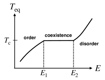
Figure 2: Schematic graph of $T_{\rm eq}$ as a function of $E$. The phase coexistence is observed at $T_{\rm eq}=T_{c}$ for $E_{1}\leq E\leq E_{2}$.

Now, we define the momentum density field $v({\boldsymbol{r}})$ conjugate to ${m}({\boldsymbol{r}})$ as

$$v\equiv\partial_{t}m.$$ (II.17)

The energy density field $\phi({\boldsymbol{r}})$ consists of the internal energy density field $u({\boldsymbol{r}})$, the kinetic energy of the order parameter density $v({\boldsymbol{r}})^{2}/2$, and the energy contribution of the order parameter density gradient which is most relevant in the interface. Note that $v({\boldsymbol{r}})^{2}/2$ is separated from $u({\boldsymbol{r}})$, which is standard in fluid dynamics Landau-Lifshitz-Fluid . That is, $\phi({\boldsymbol{r}})$ is expressed as

$$\phi({\boldsymbol{r}})=u({\boldsymbol{r}})+\frac{v({\boldsymbol{r}})^{2}}{2}+\frac{d_{e}}{2}|{\boldsymbol{\nabla}}m|^{2},$$ (II.18)

where $d_{e}$ is assumed to be constant, for simplicity. The energy conservation is now written as

$$\int d^{3}{\boldsymbol{r}}\phi({\boldsymbol{r}})=E.$$ (II.19)

We consider the entropy functional ${\cal S}$ as a functional of $(m,v,\phi)$ with the energy conservation (II.19). Explicitly, we express

$${\cal S}(m,v,\phi)$$

$$=\int d^{3}{\boldsymbol{r}}\left[s\left(\phi({\boldsymbol{r}})-\frac{v({\boldsymbol{r}})^{2}}{2}-\frac{d_{e}}{2}|{\boldsymbol{\nabla}}m|^{2},m({\boldsymbol{r}})\right)\right.$$

$$\quad\left.-\frac{d_{s}}{2}|{\boldsymbol{\nabla}}m|^{2}\right].$$ (II.20)

The entropy functional including the gradient term was used in Refs. Penrose ; HHM . The same concept naturally appears in the hydrodynamic equations with the interface thermodynamics Onuki ; Fujitani . The entropy functional in Ref. Fukuma-Sakatani also takes a similar form, but it employs the gradient expansion around the global equilibrium which is different from the gradient expansion around the local equilibrium shown in (II.20).

Related to $u^{\rm o}$ and $u^{\rm d}$, it is useful to introduce the heat capacity $c^{\rm o/d}$ without an external field defined as

$$c^{\rm o}(T) \equiv \frac{du(T,m_{\rm loc}(T))}{dT},$$ (II.21)

$$c^{\rm d}(T) \equiv \frac{du(T,m=0)}{dT}.$$ (II.22)

We also define the entropy densities as

$$s^{\rm o}(T) \equiv s(T,m_{\rm loc}(T)),$$ (II.23)

$$s^{\rm d}(T) \equiv s(T,m=0).$$ (II.24)

We then have

$$c^{\rm o}(T) = T\frac{ds^{\rm o}(T)}{dT},$$ (II.25)

$$c^{\rm d}(T) = T\frac{ds^{\rm d}(T)}{dT}.$$ (II.26)

II.2 Deterministic dynamics for equilibrium cases

For the entropy functional ${\cal S}$ in (II.20), we calculate the functional derivative as

$$\frac{\delta\cal S}{\delta m({\boldsymbol{r}})}=\left({\frac{\partial s}{\partial m}}\right)_{u}+d_{e}({\boldsymbol{\nabla}}\beta)({\boldsymbol{\nabla}}m)+\beta d_{f}\Delta m,$$ (II.27)

$$\frac{\delta\cal S}{\delta v({\boldsymbol{r}})}=-{\beta v},$$ (II.28)

$$\frac{\delta\cal S}{\delta\phi({\boldsymbol{r}})}=\beta.$$ (II.29)

Here, we have defined the coefficient of the gradient contribution to the free energy density as

$$d_{f}\equiv d_{e}+Td_{s}$$ (II.30)

with constants $d_{e}$ and $d_{s}$. From (II.17) and (II.28), we have

$$\partial_{t}m=-T\frac{\delta\cal S}{\delta v({\boldsymbol{r}})}.$$ (II.31)

Since the right-hand side of (II.31) is a reversible term that yields no entropy production, $\partial_{t}v$ should contain a corresponding reversible term. We then assume that the simplest momentum dissipation term $-\gamma v$ is contained in $\partial_{t}v$, where $\gamma$ is assumed to be a positive constant. That is, using (II.28) and (II.31), we write

$$\partial_{t}v=\gamma T\frac{\delta\cal S}{\delta v({\boldsymbol{r}})}+T\frac{\delta\cal S}{\delta m({\boldsymbol{r}})}.$$ (II.32)

Finally, from the energy conservation (II.19), we assume the minimum form of the time evolution of $\phi$:

$$\partial_{t}\phi=-{\boldsymbol{\nabla}}\left(\lambda{\boldsymbol{\nabla}}\frac{\delta\cal S}{\delta\phi({\boldsymbol{r}})}\right),$$ (II.33)

where $\lambda$ is a function of $(T,m)$. The thermal conductivity $\kappa$ is related to $\lambda$ as

$$\kappa=\frac{\lambda}{T^{2}}.$$ (II.34)

For the model (II.31), (II.32) and (II.33), we confirm the monotonic increment of ${\cal S}$ in time, which is explicitly calculated as

$$\frac{d\cal S}{dt} =\int d^{3}{{\boldsymbol{r}}}\left[\frac{\delta\cal S}{\delta m}\partial_{t}m+\frac{\delta\cal S}{\delta v}\partial_{t}v+\frac{\delta\cal S}{\delta\phi}\partial_{t}\phi\right]$$

$$=\int d^{3}{{\boldsymbol{r}}}\left[\gamma T\left(\frac{\delta\cal S}{\delta v({\boldsymbol{r}})}\right)^{2}+\lambda\left|{\boldsymbol{\nabla}}\frac{\delta\cal S}{\delta\phi({\boldsymbol{r}})}\right|^{2}\right]$$

$$\qquad-\int d^{3}{{\boldsymbol{r}}}{\boldsymbol{\nabla}}(\beta\lambda{\boldsymbol{\nabla}}\beta)$$

$$=\int d^{3}{{\boldsymbol{r}}}\left[\gamma T\left(\frac{\delta\cal S}{\delta v({\boldsymbol{r}})}\right)^{2}+\lambda\left|{\boldsymbol{\nabla}}\frac{\delta\cal S}{\delta\phi({\boldsymbol{r}})}\right|^{2}\right]$$

$$\geq 0,$$ (II.35)

where we have used the adiabatic condition

$$({\boldsymbol{\nabla}}\beta){\boldsymbol{n}}=0$$ (II.36)

at the boundaries with the unit normal vector ${\boldsymbol{n}}$. The expression (II.35) shows that the right-hand side of (II.31) and the second term in the right-hand side of (II.32) yield no entropy production.

By substituting (II.27), (II.28) and (II.29) into the equations (II.31), (II.32), and (II.33), we obtain the explicit form of the equations as

$$\partial_{t}m={v},$$ (II.37)

$$\partial_{t}v=-\gamma v+\sigma+Td_{e}({\boldsymbol{\nabla}}\beta)({\boldsymbol{\nabla}}m)+d_{f}\Delta m,$$ (II.38)

$$\partial_{t}\phi=-{\boldsymbol{\nabla}}\left(\lambda{\boldsymbol{\nabla}}\beta\right),$$ (II.39)

where the thermodynamic force $\sigma$ is given by

$$\sigma=T\left({\frac{\partial s}{\partial m}}\right)_{u}.$$ (II.40)

See (II.6). From the thermodynamic relation

$$-\left({\frac{\partial f}{\partial m}}\right)_{T}=T\left({\frac{\partial s}{\partial m}}\right)_{u},$$ (II.41)

one can rewrite the thermodynamic force $\sigma$ as

$$\sigma=-\left({\frac{\partial f}{\partial m}}\right)_{T}.$$ (II.42)

By using (II.18) and (II.38), we can express the last equation (II.39) for the case that $d_{e}=d_{s}=0$ as

$$\partial_{t}u={\gamma v^{2}}-\sigma\partial_{t}m-{\boldsymbol{\nabla}}(\lambda{\boldsymbol{\nabla}}\beta).$$ (II.43)

The first term of the right-hand side represents the generating heat caused by the momentum dissipation, the second term is associated with the work done by the thermodynamic force, and the third term the heat conduction.

The parameters $d_{e}$ and $d_{f}$ characterize the interface energy and the interface free energy, respectively. Let us estimate the magnitude of $d_{e}$ and $d_{f}$. We first discuss the interface width in the mesoscopic description. Physically, the interface is identified as a deformed surface of an intrinsic width $w$ which is at most $10^{-7}$ cm width . This width $w$ is of the same order as the microscopic length $\ell$, and the deformation of the surface is described by a capillary wave theory or fluctuation theory Triez-Zwanzig . By averaging density profiles in the equilibrium ensemble, one has an effective interface of the width $w_{\rm eff}$ which is estimated as $w_{\rm eff}\simeq\ell\sqrt{\log(L/\ell)}$ for three-dimensional systems Weeks . We note here that $w_{\rm eff}/L\to 0$ in the limit $\eta\to 0$. That is, the interface in the deterministic hydrodynamic equation is a singular surface whose motion has been formulated as a free boundary problem Anderson98 , but it should be noted that when we keep the finiteness of the interface width in the dynamics, the noise intensity also remains finite. In the mesoscopic description we employ, all thermodynamic quantities are spatially averaged over a region with the mesoscopic length $\Lambda$. Thus, the interface width of the spatially averaged configuration is given by the mesoscopic length $\Lambda$ up to a multiplicative numerical constant, as shown in Fig. 3. Then, since a typical value of $d_{f}|{\boldsymbol{\nabla}}m|^{2}$ in the interface region is estimated as $T_{c}\ell^{-3}$, we have

$$d_{f}\frac{m_{*}^{2}}{\Lambda^{2}}\simeq T_{c}\ell^{-3},$$ (II.44)

where $m_{*}$ is the characteristic value of $m$ in the ordered state and $\ell$ represents the microscopic length scale mentioned in the first paragraph of Sec. II.1.

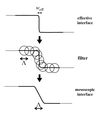
Figure 3: The statistical average of a single interface is represented by an effective interface whose width remains microscopic. By the spatial average over a region of length $\Lambda$, the interface in the mesoscopic description is defined.

II.3 Stochastic dynamics for equilibrium cases

A collection of the configurations $m$, $v$, and $\phi$ is denoted by

$$\alpha=(m,v,\phi).$$ (II.45)

Recalling that the system is enclosed by the adiabatic wall, we construct a stochastic model that yields the stationary distribution

$${\cal P}_{\rm eq}(\alpha)={\cal N}\exp({\cal S}(\alpha))\delta\left(\int d^{3}{\boldsymbol{r}}\phi({\boldsymbol{r}})-E\right)$$ (II.46)

for the equilibrium case, where ${\cal N}$ is the normalization constant. It should be noted that the energy conservation (II.19) holds for the stochastic systems. We add Gaussian white noises to (II.37), (II.38), and (II.39) that satisfy the detailed balance condition. The noise intensity is related to the dissipation intensity, which is called the fluctuation-dissipation relation of the second kind. We then write

$$\partial_{t}m={v},$$ (II.47)

$$\partial_{t}v=-\gamma v+\sigma+d_{e}T({\boldsymbol{\nabla}}\beta)({\boldsymbol{\nabla}}m)$$

$$\qquad\qquad+d_{f}\Delta m+\sqrt{2\gamma T}\xi^{v},$$ (II.48)

$$\partial_{t}\phi=-{\boldsymbol{\nabla}}\left(\lambda{\boldsymbol{\nabla}}\beta+\sqrt{2\lambda}{\boldsymbol{\xi}}^{\phi}\right),$$ (II.49)

where $\xi^{v}$ and ${\boldsymbol{\xi}}^{\phi}$ are Gaussian white noise. For later convenience, we set

$$\xi^{1} = 0,$$ (II.50)

$$\xi^{2} = \xi^{v},$$ (II.51)

$$(\xi^{3},\xi^{4},\xi^{5}) = {{\boldsymbol{\xi}}}^{\phi}.$$ (II.52)

The property of the Gaussian white noise is formally expressed as

$$\left\langle\xi^{a}({\boldsymbol{r}},t)\xi^{b}({\boldsymbol{r}}^{\prime},t^{\prime})\right\rangle = \delta^{ab}\delta({\boldsymbol{r}}-{\boldsymbol{r}^{\prime}})\delta(t-t^{\prime}),$$ (II.53)

where $2\leq a,b\leq 5$. It should be noted that the argument so far is too formal. Indeed, due to the multiplicative nature of the noise, the formal model exhibits a singular behavior. In Appendix B, we perform a careful analysis of the stochastic process.

Historically, a deterministic order parameter model with energetics was derived from an entropy functional as a phase field model that describes crystal growth Penrose . From this direction of research, one may interpret the model we study as a phase field model with noise. The equations in this previous study correspond to the over-damped version of (II.37), (II.38), and (II.39) with $d_{e}=0$. Similar equations were also considered in the context of critical phenomena HHM , where another simple entropy functional is assumed differently from our case. The model in this previous study HHM , where the noise was taken into account, was called Model C HH .

II.4 Scaling

We consider a dimensionless form of the equations (II.47), (II.48), and (II.49). First, we define the dimensionless quantity $\breve{Q}$ for any quantity $Q$ by

$$Q=\breve{Q}Q_{*},$$ (II.54)

where $Q_{*}$, which is a characteristic value with the dimension, is estimated below. We then introduce dimensionless space coordinate $\breve{{\boldsymbol{r}}}$ and dimensionless time $\breve{t}$ so that the relaxation time of thermodynamic quantities, which is denoted by $\tau$, becomes the unity in this dimensionless time $\breve{t}$. That is, we set

$$({\boldsymbol{r}},t)=(L\breve{{\boldsymbol{r}}},\tau\breve{t}).$$ (II.55)

Note that the choice of dimensionless coordinates $(\breve{{\boldsymbol{r}}},\breve{t})$ is arbitrary, and we choose this macroscopic unit for later convenience. This is in contrast with $\breve{Q}$, which is determined by the physical properties of natural phenomena.

By substituting (II.54) and (II.55) into (II.47), (II.48) and (II.49), we have

$$\partial_{\breve{t}}\breve{m}=\Gamma_{1}\breve{v},$$ (II.56)

$$\partial_{\breve{t}}\breve{v}=-\Gamma_{2}\breve{v}+\Gamma_{3}\breve{\sigma}+\Gamma_{4}\left[\breve{T}\breve{d}_{e}(\breve{{\boldsymbol{\nabla}}}\breve{\beta})(\breve{{\boldsymbol{\nabla}}}\breve{m})+\breve{d}_{f}\breve{\Delta}\breve{m}\right]$$

$$\qquad\qquad+\sqrt{2\Gamma_{5}\breve{T}}\breve{\xi}^{v},$$ (II.57)

$$\partial_{\breve{t}}\breve{\phi}=-\breve{{\boldsymbol{\nabla}}}\left(\Gamma_{6}\breve{\lambda}\breve{{\boldsymbol{\nabla}}}\breve{\beta}+\sqrt{2\breve{\lambda}\Gamma_{7}}\breve{{\boldsymbol{\xi}}}^{\phi}\right),$$ (II.58)

where we have introduced dimensionless parameters

$$(\Gamma_{1},\Gamma_{2},\Gamma_{3},\Gamma_{4},\Gamma_{5},\Gamma_{6},\Gamma_{7})$$

$$=\left(\frac{v_{*}\tau}{m_{*}},\gamma\tau,\frac{\sigma_{*}\tau}{v_{*}},\frac{(d_{f})_{*}m_{*}\tau}{L^{2}v_{*}},\frac{\gamma T_{*}\tau}{L^{3}v_{*}^{2}},\frac{\lambda_{*}\beta_{*}\tau}{L^{2}\phi_{*}},\frac{\lambda_{*}\tau}{L^{5}\phi_{*}^{2}}\right).$$ (II.59)

Here, we have assumed $(d_{e})_{*}=(d_{f})_{*}$ from (II.30). The characteristic values of the quantities are estimated by using $T_{c}$, $\tau$, $L$, and the microscopic length $\ell$. Concretely, first, it is obvious $T_{*}=T_{c}$. Second, from the equipartition law, $\phi_{*}$ is estimated as $T_{c}\ell^{-3}$ up to a multiplicative numerical constant. From (II.17) and (II.18), we find that $v_{*}^{2}=\phi_{*}$ and $m_{*}=\tau v_{*}$; and from (II.42), we have $\sigma_{*}=\phi_{*}/m_{*}$. Finally, since $\lambda$ determines the diffusion time scale of the energy, we obtain

$$\lambda_{*}=T_{c}\phi_{*}\frac{L^{2}}{\tau}.$$ (II.60)

From (II.44), we also have

$$(d_{f})_{*}=\frac{\Lambda^{2}}{m_{*}^{2}}T_{c}\ell^{-3}.$$ (II.61)

By substituting these results, we obtain

$$(\Gamma_{1},\Gamma_{2},\Gamma_{3},\Gamma_{4},\Gamma_{5},\Gamma_{6},\Gamma_{7})=\left(1,\breve{\gamma},1,\eta,\breve{\gamma}\eta^{3},1,\eta^{3}\right),$$ (II.62)

where we set $\breve{\gamma}=\gamma\tau$ and we have used $\eta$ defined by (II.3), which is assumed to be sufficiently small. Moreover, we consider the dimensionless energy $\breve{E}$ defined by

$$E=\breve{E}T_{c}\left(\frac{L}{\ell}\right)^{3}.$$ (II.63)

The mesoscopic length $\Lambda$ is also expressed as $\Lambda=\breve{\Lambda}L$, where $\breve{\Lambda}$ is written as

$$\breve{\Lambda}=\sqrt{\eta}$$ (II.64)

from (II.4).

Here, in order to simplify the notation, we remove all breve symbols. The final expression then becomes

$$\partial_{t}m=v,$$ (II.65)

$$\partial_{t}v=-\gamma v+\sigma+\eta\left[Td_{e}({\boldsymbol{\nabla}}\beta)({\boldsymbol{\nabla}}m)+d_{f}\Delta m\right]$$

$$\qquad\qquad+\sqrt{2\gamma\eta^{3}T}\xi^{v},$$ (II.66)

$$\partial_{t}\phi=-{\boldsymbol{\nabla}}\left(\lambda{\boldsymbol{\nabla}}\beta+\sqrt{2\lambda\eta^{3}}{\boldsymbol{\xi}}^{\phi}\right)$$ (II.67)

with the small parameter $\eta\ll 1$ that represents the separation of scales.

Furthermore, when we study the deterministic systems, we analyze the noiseless limit of (II.65), (II.66), (II.67):

$$\partial_{t}m=v,$$ (II.68)

$$\partial_{t}v=-\gamma v+\sigma+\eta\left[Td_{e}({\boldsymbol{\nabla}}\beta)({\boldsymbol{\nabla}}m)+d_{f}\Delta m\right]$$ (II.69)

$$\partial_{t}\phi=-{\boldsymbol{\nabla}}\left(\lambda{\boldsymbol{\nabla}}\beta\right)$$ (II.70)

instead of (II.37), (II.38), and (II.39). It should be noted that the dimensionless space coordinate $(x,y,z)$ satisfies $0\leq x\leq 1$, $0\leq y\leq L_{y}/L$, and $0\leq z\leq L_{z}/L$. Hereafter, we set

$$A=\frac{L_{y}L_{z}}{L^{2}},$$ (II.71)

which is the dimensionless area of the cross-section of the system.

When we consider a symmetry-breaking phase, the long time behavior of the system for finite $\eta$ is different from that for the system in the limit $\eta\to 0$. In order to avoid such a singular behavior, we add a small symmetry-breaking field $\sigma^{\rm ex}(x)$ to the right-hand side of (II.66), and consider the limit $\sigma^{\rm ex}(x)\to 0$ in the last step. Here, $\sigma^{\rm ex}(x)$ is spatially inhomogeneous so as to break the left-right symmetry. Specifically, we set $\sigma^{\rm ex}(x)>0$ for $x\in[0,1/2]$ and $\sigma^{\rm ex}(x)=0$ for $x\in[1/2,1]$ such that the equilibrium configuration is continuously deformed to that in the heat conduction state with $J<0$. In the argument below, we do not write this term explicitly but we always keep this process in mind.

II.5 Non-equilibrium adiabatic conditions

II.5.1 Deterministic cases

We study the heat conduction by using the equations (II.68), (II.69), and (II.70) with the boundary condition

$$\lambda\partial_{x}\beta(0,y,z)=\lambda\partial_{x}\beta(1,y,z)=J$$ (II.72)

at the boundaries $x=0$ and $x=1$ instead of (II.36), while (II.36) holds at the other boundaries. Without loss of generality, we assume $J\leq 0$. The condition (II.72) implies that the energy flux is kept constant at the boundaries. A remarkable property of the boundary condition is that the total energy of the system is conserved. From this property, we call (II.72) with $J\not=0$ a non-equilibrium adiabatic condition, which is contrasted with more standard boundary conditions $T(0,y,z)=T_{\rm L}$ and $T(1,y,z)=T_{\rm R}$. We impose the special boundary condition (II.72) for a technical reason to analyze stochastic systems.

II.5.2 Stochastic cases

We attempt to extend (II.72) to the stochastic systems. We expect the following two conditions. The first condition is that the stationary distribution is given by (II.46) when $J=0$. The second condition is that when $J\not=0$, similarly to the deterministic description, non-equilibrium nature is brought only by the boundary condition with keeping the energy conservation. Concretely, we impose the boundary condition

$$j_{x}(x=0,y,z,t) = J,$$ (II.73)

$$j_{x}(x=1,y,z,t) = J,$$ (II.74)

and ${\boldsymbol{j}}{\boldsymbol{n}}=0$ at the other boundaries, where ${\boldsymbol{j}}$ is defined as

$${\boldsymbol{j}}\equiv\lambda{\boldsymbol{\nabla}}\beta+\sqrt{2\lambda\eta^{3}}{\boldsymbol{\xi}}^{\phi}.$$ (II.75)

We easily confirm that the two conditions are satisfied by this boundary condition.

II.5.3 Linear response regime

In order to represent the extent of the non-equilibrium, we introduce a dimensionless small parameter

$$\epsilon\equiv\frac{|J|LT_{c}}{\lambda_{*}}$$ (II.76)

using the original dimensional quantities. By introducing the dimensionless heat flux $\breve{J}$ as

$$J=\breve{J}\frac{\lambda_{*}}{T_{c}L},$$ (II.77)

we find that $|\breve{J}|=\epsilon$. Therefore,

$$|J|=\epsilon$$ (II.78)

in this dimensionless form. In the argument below, we focus on the linear response regime by studying only the contribution of $O(\epsilon)$.

III Interface in the deterministic system

In this section, we study the properties of the interface in the deterministic system. In Sec. III.1, we analyze the stationary interface in the equilibrium state. In Sec. III.2, we analyze the interface in the heat conduction. In Sec. III.3, we summarize the result for the deterministic system, and we show our motivation of studying the stochastic system.

III.1 Equilibrium interface

We study the deterministic system described by (II.68), (II.69), and (II.70). For any initial value of $(m({\boldsymbol{r}}),v({\boldsymbol{r}}),\phi({\boldsymbol{r}}))$, the energy $E$ is conserved over time and $d{\cal S}/dt\geq 0$ for any $t$ as shown in (II.35). This means that $(m({\boldsymbol{r}},t),v({\boldsymbol{r}},t),\phi({\boldsymbol{r}},t))$ goes to the equilibrium value

$$\alpha_{\rm eq}({\boldsymbol{r}})=(m_{\rm eq}({\boldsymbol{r}}),v_{\rm eq}({\boldsymbol{r}})=0,\phi_{\rm eq}({\boldsymbol{r}})),$$ (III.1)

which maximizes ${\cal S}(\alpha)$ under the energy conservation. In particular, when $E_{1}\leq E\leq E_{2}$, where $E_{1}$ and $E_{2}$ are given by (II.13) and (II.14), the equilibrium temperature takes the constant value $T_{c}$ as shown in Fig. 2. In this equilibrium state, the temperature is homogeneous in space such that $T({\boldsymbol{r}})=T_{c}$, while $(u_{\rm eq}({\boldsymbol{r}}),m_{\rm eq}({\boldsymbol{r}}))$ is not homogeneous in space; the ordered state $(m=m_{\rm loc}(T_{c}))$ and the disordered state $(m=0)$ coexist with the minimum surface of the interface between the two states.

We derive an expression of $m_{\rm eq}({\boldsymbol{r}})$ for $E_{1}\leq E\leq E_{2}$. Since the horizontal length $L$, which is now normalized as unity, is larger than the lengths of other directions $L_{y}$ and $L_{z}$, the stationary interface is perpendicular to the $x$-axis. Furthermore, from (II.69) with (II.42), we find that the stationary interface described by $m=m_{\rm eq}(x)$ satisfies

$$-\frac{\partial f(T_{c},m)}{\partial m}+\eta d_{f}\partial_{x}^{2}m=0$$ (III.2)

with the boundary conditions (II.9). Let $X_{\rm eq}$ be the stationary interface position for a given value of the total energy $E$, as shown in Fig. 4. We consider the case that the ordered state appears on the left-side. Then, $X_{\rm eq}$ is determined by

$$X_{\rm eq}u^{\rm o}(T_{c})+(1-X_{\rm eq})u^{\rm d}(T_{c})=\frac{E}{A}$$ (III.3)

in the limit $\eta\to 0$. Looking at (III.2), we express the solution of (III.2) with $\eta\ll 1$ as

$$m_{\rm eq}(x)=\bar{\bar{m}}\left(\frac{x-X_{\rm eq}}{\sqrt{\eta}}\right)m_{\rm loc}(T_{c}).$$ (III.4)

The quantity $\bar{\bar{m}}(\xi)$, which describes an internal structure of the interface, then satisfies

$$-\frac{\partial f(T_{c},\bar{\bar{m}}m_{\rm loc}(T_{c}))}{\partial\bar{\bar{m}}}+{m_{\rm loc}^{2}(T_{c})d_{f}}\partial_{\xi}^{2}\bar{\bar{m}}=0$$ (III.5)

with $\xi=(x-X_{\rm eq})/\sqrt{\eta}$, $\bar{\bar{m}}(0)=1/2$, $\bar{\bar{m}}(-\infty)=1$, $\bar{\bar{m}}(\infty)=0$.

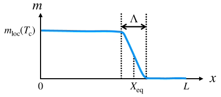
Figure 4: Schematic figure of a stationary interface in equilibrium. $\Lambda=\sqrt{\eta}$ and $L=1$ in the dimensionless form.

III.2 Interface in the heat conduction steady state

In this section, we derive the stationary interface in the heat conduction based on the deterministic description. That is, from (II.68), (II.69), and (II.70) with (II.42), we find that the stationary solution satisfies

$$-\left({\frac{\partial f}{\partial m}}\right)_{T}+\eta Td_{e}(\partial_{x}\beta)(\partial_{x}m)+\eta d_{f}\partial_{x}^{2}m =0,$$ (III.6)

$$\lambda\partial_{x}\beta =J,$$ (III.7)

which are interpreted as the non-equilibrium extension of (III.2).

We analyze the equations (III.6) and (III.7). Let $X_{\rm ss}$ be the position of the stationary interface for $(E,J)$. We then determine the temperature of the interface $\theta$ from (III.6) and (III.7) with $X_{\rm ss}$. Multiplying $(\partial_{x}m)$ to (III.6) and integrating it over $I\equiv[X_{\rm ss}-M\sqrt{\eta},X_{\rm ss}+M\sqrt{\eta}]$ with a large $M$ independent of $\eta$, we obtain

$$-\int_{I}dx(\partial_{x}m)\left({\frac{\partial f}{\partial m}}\right)_{T}+\eta\int_{I}dxTd_{e}(\partial_{x}\beta)(\partial_{x}m)^{2}$$

$$\qquad+\eta\int_{I}dxd_{f}(\partial_{x}m)(\partial_{x}^{2}m)=0.$$ (III.8)

Here, we note

$$\partial_{x}f=\left({\frac{\partial f}{\partial T}}\right)_{m}\partial_{x}T+\left({\frac{\partial f}{\partial m}}\right)_{T}\partial_{x}m$$ (III.9)

and

$$d_{f}(\partial_{x}m)(\partial_{x}^{2}m)=\frac{d_{f}}{2}\partial_{x}((\partial_{x}m)^{2})$$

$$\qquad\qquad=\frac{1}{2}\partial_{x}(d_{f}(\partial_{x}m)^{2})-\frac{d_{s}}{2}(\partial_{x}T)(\partial_{x}m)^{2}.$$ (III.10)

By using these results, we further rewrite (III.8) as

$$f(X_{\rm ss}+M\sqrt{\eta})-f(X_{\rm ss}-M\sqrt{\eta})$$

$$~{}~{}=J\int_{X_{\rm ss}-M\sqrt{\eta}}^{X_{\rm ss}+M\sqrt{\eta}}dx\left[\frac{T\eta d_{e}(\partial_{x}m)^{2}}{\lambda}+\frac{T^{2}\eta d_{s}(\partial_{x}m)^{2}}{2\lambda}\right]$$

$$~{}~{}~{}~{}-\int_{X_{\rm ss}-M\sqrt{\eta}}^{X_{\rm ss}+M\sqrt{\eta}}dxs\partial_{x}T$$

$$~{}~{}~{}~{}+\frac{d_{f}}{2}\left.(\partial_{x}m)^{2}\right|_{X_{\rm ss}-M\sqrt{\eta}L}^{X_{\rm ss}+M\sqrt{\eta}L}.$$ (III.11)

The last term is proportional to $\epsilon^{2}$, because

$$\partial_{x}m\simeq-\frac{dm_{\rm loc}(T)}{dT}T^{2}\frac{J}{\lambda}$$ (III.12)

at $x=X_{\rm ss}-M\sqrt{\eta}$, and $\partial_{x}m=0$ at $x=X_{\rm ss}+M\sqrt{\eta}$. The first line of the right-hand side of (III.11) is rewritten as

$$J\int_{X_{\rm ss}-M\sqrt{\eta}}^{X_{\rm ss}+M\sqrt{\eta}}dx\eta\frac{T(d_{e}+Td_{s}/2)(\partial_{x}m)^{2}}{\lambda}.$$ (III.13)

This is estimated as

$$\epsilon{\eta}^{\frac{1}{2}}d_{f}m_{\rm loc}(T_{c})^{2}$$ (III.14)

up to a numerical factor when $\lambda$ in the interface region is estimated as $\lambda_{*}$. Thus, the first line of (III.11) is $O(\eta^{1/2})$. From these, the leading term of (III.11) becomes

$$f(X_{\rm ss}+M\sqrt{\eta})-f(X_{\rm ss}-M\sqrt{\eta})=-\int_{X_{\rm ss}-M\sqrt{\eta}}^{X_{\rm ss}+M\sqrt{\eta}}dxs(\partial_{x}T).$$ (III.15)

Furthermore, recalling $f=u-Ts$, we have

$$u(X_{\rm ss}+M\sqrt{\eta})-u(X_{\rm ss}-M\sqrt{\eta})=\int_{X_{\rm ss}-M\sqrt{\eta}}^{X_{\rm ss}+M\sqrt{\eta}}dxT(\partial_{x}s).$$ (III.16)

Let $\theta$ be the temperature of the interface, defined by

$$\theta=T(X_{\rm ss}).$$ (III.17)

Noting the continuity of $T(x)$ and ignoring $O(\eta^{1/2})$ terms, we find that (III.16) becomes

$$u^{\rm o}(\theta)-u^{\rm d}(\theta)=\theta[s^{\rm o}(\theta)-s^{\rm d}(\theta)],$$ (III.18)

where $u^{\rm o}$ and $u^{\rm d}$ are defined by (II.15) and (II.16). $s^{\rm o}$ and $s^{\rm d}$ are also defined by (II.23) and (II.24). We thus obtain

$$\theta=T_{c}+O({\eta}^{\frac{1}{2}}).$$ (III.19)

This estimate indicates that, in the limit $\eta\to 0$ with $\epsilon$ fixed, the stationary interface temperature in the heat conduction state remains $T_{c}$.

III.3 Role of fluctuation

If the deterministic equation correctly describes the thermodynamic behavior, all thermodynamic quantities are determined from the stationary solution of the equation. In particular, the interface temperature in the heat conduction systems is equal to the equilibrium transition temperature in the limit $\eta\to 0$. Now, the question is whether or not the deterministic equation is valid for the phase coexistence under heat conduction.

As a related example, let us recall the understanding of a fluid consisting of many particles in two dimensions. One may write the standard two-dimensional hydrodynamic equation as a deterministic model describing the hydrodynamic behavior. However, it has been known that the parameters in the equation, the transportation coefficients, do not have a definite value measured in experiments. Theoretically, this result is understood as a singular (divergent) behavior of the parameter values in the macroscopic limit on the basis of microscopic dynamics. In this sense, deterministic hydrodynamic equations are not valid for describing the dynamical behaviors of a fluid consisting of many particles in two dimensions. Even for this case, it is expected that stochastic hydrodynamic equations with well-defined parameters can describe the behavior quantitatively. The consistency between the two models has been understood from the renormalization group analysis FNS .

In the phase coexistence under heat conduction, the interface region is singular because the interface width is $O(\sqrt{\eta})$. Thermodynamic quantities in this thin interface region may be described by equilibrium statistical mechanics. Here we discuss how an energy fluctuation of $O(\sqrt{\eta})$ in the ordered region evolves over time under the equilibrium condition. The corresponding temperature fluctuation in the ordered region is $O(\sqrt{\eta})$ because the heat capacity is $O(1)$. Then the energy flows into the interface region and this leads to the temperature change of $O(\sqrt{\eta})$ in the interface region, which is achieved by the change in the interface position of $O(\sqrt{\eta})$. Since the temperature difference over the interface region is estimated as $O(\sqrt{\eta})$, $\partial_{x}\beta$ in the interface region is $O(1)$. Thus, the energy flux in the interface region is expressed as $\lambda_{\rm int}\times O(1)$, where $\lambda_{\rm int}$ is the thermal conductivity in the interface region. Since the energy flux of $O(\sqrt{\eta})$ in the bulk is balanced with the energy flux in the interface region, it is expected $\lambda_{\rm int}=O(\sqrt{\eta})$. That is, the singularity appears in the limit $\eta\to 0$.

When we study the deterministic system (II.68), (II.69), and (II.70) with $\lambda_{\rm int}=O(\sqrt{\eta})$, the behavior depends on the detail of $\lambda_{\rm int}$ even in the limit $\eta\to 0$. For example, for heat conduction steady state, the temperature gap of $O(1)$ appears and the amount of the gap depends on $\lambda_{\rm int}/\sqrt{\eta}$ in the limit $\eta\to 0$. Here, let us recall that the energy transfer from/to the interface region to/from the bulk is basically induced by fluctuations of the interface. Therefore, the stochastic noise is inevitable for the description of the energy transfer. Even if we assume that the “bare conductivity” in the interface region, which is a parameter of the stochastic model, is $O(\sqrt{\eta})$, the “measured conductivity” in the interface region may be $O(1)$ as the result of the renormalization of fluctuations. This leads to no temperature gap in the limit $\eta\to 0$, but this is not described as the limit $\eta\to 0$ of a deterministic equation. It should be noted that the energy transfer occurs as the result of fluctuations of the interface position is similar to the so-called adiabatic piston problem Callen ; Feynman ; Lieb ; Gruber ; Gruber2 .

IV Stationary distribution for interface configurations

We start this section with the Zubarev-Mclennan representation of the stationary distribution for heat conduction systems in Sec. IV.1. The probability density is an extension of the micro-canonical ensemble and we naturally define a modified entropy which contains a correction term ${\cal I}$ in addition to the entropy ${\cal S}$. Note that ${\cal I}$ is the time integration of the entropy production. Then, for a single interface configuration $\alpha_{X}$ defined in Sec. IV.2, we attempt to express ${\cal I}$ as a form without the time integration. If it is done successfully, we can formulate the variational principle so that all thermodynamic quantities can be determined as that maximizing the modified entropy. We thus attempt to evaluate ${\cal I}$. Concretely, in Sec. IV.3, we decompose ${\cal I}$ into the bulk contribution and the interface contribution. Then, in Sec. IV.4, we estimate the bulk contribution to ${\cal I}$. This will be done quite easily thanks to the boundary condition we impose. This calculation also gives the correction term ${\cal I}$ for configurations without interfaces. In Sec. IV.5, we argue that the temperature gap of $O(\sqrt{\eta})$ gives a contribution to ${\cal I}$.

IV.1 Zubarev-Mclennan representation

Let ${\cal P}_{\rm ss}(\alpha;E,J)$ be the stationary distribution of $\alpha$ for a system with $(E,J)$, where $E$ and $J$ are values of the dimensionless total energy and the dimensionless boundary current, respectively. In this subsection, we derive an expression of ${\cal P}_{\rm ss}(\alpha;E,J)$, which is called the Zubarev-Mclennan representation Zubarev ; Mclennan ; KN ; KNST-rep ; Maes-rep , in the linear response regime around the equilibrium state.

Let $\hat{\alpha}$ denote the trajectory of $\alpha$ from $t=0$ to $t=t_{f}$. That is, $\hat{\alpha}=(\alpha(t))_{t=0}^{t_{f}}$. The probability density (measure) of trajectory $\hat{\alpha}$ with $\alpha(0)$ fixed at $t=0$ is denoted by $\hat{\cal P}(\hat{\alpha}|\alpha(0);E,J)$. From (II.65), (II.66), and (II.67), we obtain

$$\log\hat{\cal P}(\hat{\alpha}|\alpha(0);E,J)=-\frac{1}{\eta^{3}}\hat{\cal I}(\hat{\alpha}|\alpha(0);E,J)+{\rm const}$$ (IV.1)

with

$$\hat{\cal I}(\hat{\alpha}|\alpha(0);E,J)=\int_{0}^{t_{f}}dt\int d^{3}{\boldsymbol{r}}\left\{\frac{1}{4\lambda}\left|{\boldsymbol{j}}-\lambda{\boldsymbol{\nabla}}\beta\right|^{2}\right.$$

$$+\left.\frac{1}{4\gamma T}\left[\partial_{t}v+\gamma v-\sigma-\eta\left(Td_{e}({\boldsymbol{\nabla}}\beta)({\boldsymbol{\nabla}}m)+d_{f}\Delta m\right)\right]^{2}\right\},$$ (IV.2)

where $\partial_{t}m$ and $\partial_{t}\phi$ are connected to $v$ and ${\boldsymbol{j}}$ as

$$\partial_{t}m-{v} = 0,$$ (IV.3)

$$\partial_{t}\phi+{\boldsymbol{\nabla}}{\boldsymbol{j}} = 0.$$ (IV.4)

By a standard technique related to the local detailed balance condition, which is reviewed in Appendix C, we can derive

$${\cal P}(\alpha,t_{f};E,J)={\cal N}{\rm e}^{{\cal S}(\alpha)/\eta^{3}}$$

$$\times\left\langle{\rm e}^{J/\eta^{3}\int d^{2}{\boldsymbol{r}}_{\perp}\int_{0}^{t_{f}}dt(\beta(1,{\boldsymbol{r}}_{\perp},t)-\beta(0,{\boldsymbol{r}}_{\perp},t))}\right\rangle_{\alpha^{\dagger}\to*}^{-J}$$

$$\times\delta\left(\int d^{3}{\boldsymbol{r}}\phi({\boldsymbol{r}})-E\right)$$ (IV.5)

with ${\boldsymbol{r}}_{\perp}=(y,z)$, where $\left\langle\ \right\rangle_{\alpha^{\dagger}\to*}^{-J}$ represents the expectation value over trajectories $\alpha(t)$ starting from $\alpha(0)=\alpha^{\dagger}=(m,-v,\phi)$ for $\alpha=(m,v,\phi)$ with respect to the path probability density in the system with $-J$.

Here, we consider the steady state obtained in the long time limit $t_{f}\to\infty$ for the system with the separation of scales $\eta\to 0$, with focusing on the linear response regime in $J$. That is, precisely speaking, three limits $t_{f}\to\infty$, $\eta\to 0$, and $\epsilon=|J|\to 0$, should be taken into account. (In addition to those, the symmetry breaking external field $\sigma^{\rm ex}(x)$ should be taken to be zero in the last step, as discussed in the previous section.) Now, if we first took the limit $t_{f}\to\infty$ for fixed $\eta$, we could not observe the symmetry breaking in the limit $\sigma^{\rm ex}(x)\to 0$. On the other hand, if we first took $\eta\to 0$, the interface motion could not be observed even in the equilibrium system, as reviewed in Appendix D. More explicitly, let $\tau_{\rm int}$ be the time scale of the interface motion. We then confirm that $\tau_{\rm int}\to\infty$ for $\eta\to 0$. See (D.27). The proper limit may be that we first set $t_{f}=K\tau_{\rm int}$ in the limit $\eta\to 0$ with fixed $K$, and take the limit $K\to\infty$. We then consider the limit $\epsilon\to 0$.

Keeping this remark in mind, we define a modified entropy $\tilde{\cal S}$ as

$$\tilde{\cal S}(\alpha;E,J)\equiv\lim_{K\to\infty}\lim_{\eta\to 0}\eta^{3}\log\frac{{\cal P}(\alpha,K\tau_{\rm int};E,J)}{{\cal N}\delta\left(\int d^{3}{\boldsymbol{r}}\phi({\boldsymbol{r}})-E\right)}.$$ (IV.6)

We then assume that the stationary probability distribution in our problem is expressed as

$${\cal P}_{\rm ss}(\alpha;E,J)={\cal N}{\rm e}^{\frac{1}{\eta^{3}}\tilde{\cal S}(\alpha;E,J)}\delta\left(\int d^{3}{\boldsymbol{r}}\phi({\boldsymbol{r}})-E\right).$$ (IV.7)

Now, recalling (II.78), we expand $\tilde{S}$ in $J$ as

$$\tilde{\cal S}(\alpha;E,J)={\cal S}_{0}(\alpha)+J{\cal I}(\alpha;E)+O(\epsilon^{2})$$ (IV.8)

with

$${\cal S}_{0}(\alpha)=\lim_{\eta\to 0}{\cal S}(\alpha).$$ (IV.9)

Here, the functional ${\cal I}$ is calculated as

$${\cal I}(\alpha;E)= \lim_{K\to\infty}\lim_{\eta\to 0}\int d^{2}{\boldsymbol{r}}_{\perp}\int_{0}^{K\tau_{\rm int}}dt$$ (IV.10)

$$\times\left\langle(\beta(1,{\boldsymbol{r}}_{\perp},t)-\beta(0,{\boldsymbol{r}}_{\perp},t))\right\rangle_{\alpha^{\dagger}\to*}^{\rm eq},$$

where $\left\langle\ \right\rangle_{\alpha\to*}^{\rm eq}$ is defined as

$$\left\langle\ \right\rangle_{\alpha\to*}^{\rm eq}=\lim_{J^{\prime}\to 0}\left\langle\ \right\rangle_{\alpha\to*}^{-J^{\prime}}.$$ (IV.11)

Note that the right-hand side is uniquely determined in the limit $J^{\prime}\to 0$ for $\sigma^{\rm ex}(x)$ fixed. (IV.7) may be referred to as the Zubarev-Mclennan representation of the probability density for the system with the flux control. When $J=0$, ${\cal P}_{\rm ss}(\alpha;E,J=0)$ is the micro-canonical distribution. The second term of (IV.8) is the non-equilibrium correction to the entropy, which represents the entropy production in the relaxation process to the equilibrium state from $\alpha^{\dagger}$ for the configuration $\alpha$. This entropy production is called excess entropy production.

IV.2 Interface configuration

In this section, we define a single interface configuration $\alpha_{X}$ whose interface position is given by $X$.

First, we introduce the over-bar to represent the average over vertical directions to the heat flux. For example,

$$\bar{\beta}(x,t)\equiv\frac{1}{A}\int d^{2}{\boldsymbol{r}}_{\perp}\beta(x,{\boldsymbol{r}}_{\perp},t),$$ (IV.12)

where $A$ is the dimensionless cross-section defined by (II.71). Let $\alpha_{X}$ denote a single interface configuration with the interface position $X$. Precisely, the interface position is specified by

$${\bar{m}}(X)=\frac{m_{\rm loc}(\bar{T}(X))}{2}.$$ (IV.13)

We then define the interface region $[X_{-},X_{+}]$ by

$$X_{-} \equiv X-r\sqrt{\eta},$$ (IV.14)

$$X_{+} \equiv X+r\sqrt{\eta},$$ (IV.15)

where $r$ is a positive constant such that $e^{-r}$ is much smaller than 1, say $e^{-r}=0.01$. A single interface configuration $\alpha_{X}$ with the interface position $X$ is defined as that satisfying

$$|{\bar{m}}(x)-m_{\rm loc}(\bar{T}(x))| \leq \delta_{m}m_{\rm loc}(\bar{T}(x))$$ (IV.16)

for $x\leq X_{-}$, and

$$|{\bar{m}}(x)|\leq\delta_{m}m_{\rm loc}(\bar{T}(x))$$ (IV.17)

for $x\geq X_{+}$, where the constant $\delta_{m}$ is much smaller than $1$. We also impose that the interface configuration satisfies

$$|\bar{v}(x)|\leq\delta_{v},$$ (IV.18)

where the constant $\delta_{v}$ is much smaller than $1$. Since we consider the limit $\eta\to 0$, the final result is independent of the parameters $(\delta_{m},\delta_{v},r)$.

For a given single interface configuration $\alpha_{X}$, we study the time evolution from $\alpha_{X}$. We assume that a configuration at any time $t$ in the time interval $[0,K\tau^{\rm int}]$ still possesses a single interface at the interface position $X(t)$ which depends on the noise realization. Note that $X(0)$ equals to $X$ in $\alpha_{X}$.

Hereafter, for simplicity, we assume

$$\lambda(T,m)=\lambda^{\rm o}$$ (IV.19)

in the ordered region $[0,X_{-}]$ and

$$\lambda(T,m)=\lambda^{\rm d}$$ (IV.20)

in the disordered region $[X_{+},1]$, where $\lambda^{\rm o}$ and $\lambda^{\rm d}$ are constants, and $\lambda(T,m)$ in the region $[X_{-},X_{+}]$ is $O(\sqrt{\eta})$, while its functional form is not specified. See Sec. III.3 for the argument.

IV.3 Correction term

We first re-write ${\cal I}$ as

$${\cal I}(\alpha_{X})=\lim_{K\to\infty}\lim_{\eta\to 0}AI(\alpha_{X}),$$ (IV.21)

where $I(\alpha_{X})$ is expressed as

$$I(\alpha_{X}) = \int_{0}^{K\tau_{\rm int}}dt\left\langle\bar{\beta}(1,t)-\bar{\beta}(0,t)\right\rangle_{\alpha_{X}^{\dagger}\to*}^{\rm eq}.$$ (IV.22)

We consider the decomposition of $I(\alpha_{X})$:

$$I(\alpha_{X})=I^{\rm o}(\alpha_{X})+I^{\rm d}(\alpha_{X})+I^{\rm int}(\alpha_{X}),$$ (IV.23)

where

$$I^{\rm o}(\alpha_{X}) \equiv \int_{0}^{K\tau_{\rm int}}dt\left\langle\bar{\beta}(X_{-},t)-\bar{\beta}(0,t)\right\rangle_{\alpha_{X}^{\dagger}\to*}^{\rm eq},$$ (IV.24)

$$I^{\rm d}(\alpha_{X}) \equiv \int_{0}^{K\tau_{\rm int}}dt\left\langle\bar{\beta}(1,t)-\bar{\beta}(X_{+},t)\right\rangle_{\alpha_{X}^{\dagger}\to*}^{\rm eq},$$ (IV.25)

and

$$I^{\rm int}(\alpha_{X})\equiv\int_{0}^{K\tau_{\rm int}}dt\left\langle\bar{\beta}(X_{+},t)-\bar{\beta}(X_{-},t)\right\rangle_{\alpha_{X}^{\dagger}\to*}^{\rm eq}.$$ (IV.26)

In the evaluation of $I^{\rm o/d}(\alpha_{X})$ and $I^{\rm int}(\alpha_{X})$, we take account of only the contribution from the most probable process by ignoring fluctuations, because we consider the weak noise cases of small $\eta$. Note that, in the bulk region, $\alpha(t)$ is replaced by the solution of the deterministic equation with $\eta\to 0$, while the deterministic equation of $\bar{\beta}(X_{+\-},t)$ is not obtained by the noiseless limit of the stochastic model. In the argument below, for any fluctuating thermodynamic quantity $Q(t)$, we use the same notation $Q(t)$ to represent the most probable value with the initial condition $\alpha(0)=\alpha_{X}^{\dagger}$ under the equilibrium condition. That is, (IV.24), (IV.25), and (IV.26) are rewritten as

$$I^{\rm o}(\alpha_{X}) \equiv \int_{0}^{K\tau_{\rm int}}dt[\bar{\beta}(X_{-},t)-\bar{\beta}(0,t)],$$ (IV.27)

$$I^{\rm d}(\alpha_{X}) \equiv \int_{0}^{K\tau_{\rm int}}dt[\bar{\beta}(1,t)-\bar{\beta}(X_{+},t)],$$ (IV.28)

and

$$I^{\rm int}(\alpha_{X})\equiv\int_{0}^{K\tau_{\rm int}}dt[\bar{\beta}(X_{+},t)-\bar{\beta}(X_{-},t)].$$ (IV.29)

Below we evaluate $I^{\rm o/d}(\alpha_{X})$ and $I^{\rm int}(\alpha_{X})$ for small $\eta$ and large $K$.

IV.4 Bulk contribution

First, we express (IV.27) and (IV.28) as

$$I^{\rm o}(\alpha_{X}) = \int_{0}^{K\tau_{\rm int}}dt\int_{0}^{X_{-}(t)}dx\partial_{x}\bar{\beta}(x,t),$$ (IV.30)

$$I^{\rm d}(\alpha_{X}) = \int_{0}^{K\tau_{\rm int}}dt\int_{X_{+}(t)}^{1}dx\partial_{x}\bar{\beta}(x,t).$$ (IV.31)

Here, we find a neat idea to use a variable $\psi(x,t)$ defined by

$$\bar{\phi}(x,t)=\frac{E}{A}+\partial_{x}\psi(x,t)$$ (IV.32)

with the boundary conditions $\psi(0,t)=\psi(1,t)=0$. For a given $\bar{\phi}(x,t)$, $\psi(x,t)$ can be uniquely determined because of the energy conservation:

$$A\int_{0}^{1}dx\bar{\phi}(x,t)=E.$$ (IV.33)

We substitute (IV.32) into (II.70) and take the boundary condition (II.36) into account. We then obtain the deterministic equation of $\psi$

$$\partial_{t}\psi+\lambda^{\rm o}\partial_{x}\bar{\beta}=0$$ (IV.34)

for $x\in[0,X_{-}(t)]$ and

$$\partial_{t}\psi+\lambda^{\rm d}\partial_{x}\bar{\beta}=0$$ (IV.35)

for $x\in[X_{+}(t),1]$. Now, by using (IV.34), (IV.30) is expressed as

$$I^{\rm o}(\alpha_{X})=-\int_{0}^{K\tau_{\rm int}}dt\int_{0}^{X_{-}(t)}dx\frac{\partial_{t}\psi}{\lambda^{\rm o}}$$

$$\qquad=-\frac{1}{\lambda^{\rm o}}\int_{0}^{K\tau_{\rm int}}dt\int_{0}^{1}dxH(X_{-}(t)-x)\partial_{t}\psi,$$ (IV.36)

where $H(x)=1$ for $x>0$ and $H(x)=0$ for $x<0$. Since

$$H(X_{-}(t)-x)\partial_{t}\psi$$

$$=\partial_{t}(H(X_{-}(t)-x)\psi)-\frac{dX}{dt}\delta(X_{-}(t)-x)\psi,$$ (IV.37)

we have

$$I^{\rm o}(\alpha_{X}) =-\frac{1}{\lambda^{\rm o}}\int_{0}^{K\tau_{\rm int}}dt\int_{0}^{1}dx\partial_{t}(H(X_{-}(t)-x)\psi)$$

$$+\frac{1}{\lambda^{\rm o}}\int_{0}^{K\tau_{\rm int}}dt\int_{0}^{1}dx\frac{dX}{dt}\delta(X_{-}(t)-x)\psi.$$ (IV.38)

We rewrite it as

$$I^{\rm o}(\alpha_{X}) =\frac{1}{\lambda^{\rm o}}\left[\int_{0}^{X_{-}(0)}\!\!\!\!dx\psi_{X}(x)-\int_{0}^{X_{-}(K\tau_{\rm int})}\!\!\!\!\!\!\!\!dx\psi(x,K\tau_{\rm int})\right]$$

$$\quad+\frac{1}{\lambda^{\rm o}}\int_{0}^{K\tau_{\rm int}}dt\frac{dX}{dt}\psi(X_{-}(t),t),$$ (IV.39)

where $\psi_{X}(x)$ is determined from $\alpha_{X}$ in the argument of $I^{\rm o}$. Similarly, we obtain

$$I^{\rm d}(\alpha_{X}) =\frac{1}{\lambda^{\rm d}}\left[\int_{X_{+}(0)}^{1}\!\!\!\!dx\psi_{X}(x)-\int_{X_{+}(K\tau_{\rm int})}^{1}\!\!\!\!\!\!\!\!dx\psi(x,K\tau_{\rm int})\right]$$

$$\quad-\frac{1}{\lambda^{\rm d}}\int_{0}^{K\tau_{\rm int}}dt\frac{dX}{dt}\psi(X_{+}(t),t).$$ (IV.40)

Now, we consider the limit $\eta\to 0$ with large $K$ fixed. The interface motion is observed with the time scale $\tau_{\rm int}=O(\eta^{-1/2})$ which is much larger than the relaxation time of thermodynamic quantities. Thus, $\alpha(x,t)$ is close to the quasi-equilibrium configuration $\alpha_{X(t)}^{\rm qeq}(x)$ with the interface position $X(t)$, where the quasi-equilibrium configuration $\alpha_{X}^{\rm qeq}(x)$ is characterized by the uniform temperature $T_{X}^{\rm qeq}$ satisfying

$$Xu^{\rm o}(T_{X}^{\rm qeq})+(1-X)u^{\rm d}(T_{X}^{\rm qeq})=\frac{E}{A}.$$ (IV.41)

All thermodynamic quantities in the quasi-equilibrium state are calculated from $\alpha_{X}^{\rm qeq}(x)$.

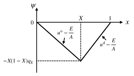
Figure 5: Example of the graph $\psi_{X}^{\rm qeq}(x)$.

As one example, the quasi-equilibrium configuration $\psi_{X}^{\rm qeq}(x)$ is given by

$$\psi_{X}^{\rm qeq}(x)=\left(u^{\rm o}(T_{X}^{\rm qeq})-\frac{E}{A}\right)x$$ (IV.42)

for $0\leq x\leq X$, and

$$\psi_{X}^{\rm qeq}(x)=-\left(u^{\rm d}(T_{X}^{\rm qeq})-\frac{E}{A}\right)(1-x)$$ (IV.43)

for $X\leq x\leq 1$. Here, we define the latent heat $q_{X}$ by

$$q_{X}\equiv u^{\rm d}(T_{X}^{\rm qeq})-u^{\rm o}(T_{X}^{\rm qeq}).$$ (IV.44)

By combining it with the relation (IV.41), we find

$$u^{\rm o}(T_{X}^{\rm qeq})-\frac{E}{A}=-(1-X)q_{X}.$$ (IV.45)

We thus have

$$\psi_{X}^{\rm qeq}(X)=-X(1-X)q_{X}.$$ (IV.46)

Summarizing these results, we show an example of quasi-equilibrium configuration $\psi_{X}^{\rm qeq}(x)$ in Fig. 5. By taking the limit $K\to\infty$ and $\eta\to 0$, we have arrived at

$$\lim_{K\to\infty}\lim_{\eta\to 0}[I^{\rm o}(\alpha_{X})+I^{\rm d}(\alpha_{X})]$$

$$=\frac{1}{\lambda^{\rm o}}\int_{0}^{X}dx\psi_{X}(x)+\frac{1}{\lambda^{\rm d}}\int_{X}^{1}dx\psi_{X}(x)$$

$$\quad-\frac{1}{\lambda^{\rm o}}\int_{0}^{X_{\rm eq}}dx\psi_{X_{\rm eq}}^{\rm qeq}(x)-\frac{1}{\lambda^{\rm d}}\int_{X_{\rm eq}}^{1}dx\psi_{X_{\rm eq}}^{\rm qeq}(x)$$

$$\quad+\int_{X}^{X_{\rm eq}}dY\psi_{Y}^{\rm qeq}(Y)\left(\frac{1}{\lambda^{\rm o}}-\frac{1}{\lambda^{\rm d}}\right).$$ (IV.47)

IV.5 Interface contribution

We next study the interface contribution (IV.29). By defining

$$\beta_{\pm}^{\rm int}(t)\equiv\bar{\beta}(X_{\pm}(t),t),$$ (IV.48)

we replace (IV.29) by

$$I^{\rm int}(\alpha_{X})=\int_{0}^{K\tau_{\rm int}}dt\left[\beta_{+}^{\rm int}(t)-\beta_{-}^{\rm int}(t)\right].$$ (IV.49)

We call $\beta^{\rm int}_{+}(t)-\beta^{\rm int}_{-}(t)$ “inverse-temperature gap”. We estimate $I^{\rm int}(\alpha_{X})$ by dividing the interval $[0,K\tau_{\rm int}]$ into two intervals $[0,t_{c}]$ and $[t_{c},K\tau_{\rm int}]$, where we take $t_{c}$ satisfying

$$1\ll t_{c}\ll\tau_{\rm int}$$ (IV.50)

for small $\eta$. The contribution to $I^{\rm int}$ in the time interval $[0,t_{c}]$ is expressed as

$$I_{1}^{\rm int}(\alpha_{X})=\int_{0}^{t_{c}}dt[\beta^{\rm int}_{+}(t)-\beta^{\rm int}_{-}(t)].$$ (IV.51)

The initial configuration $\alpha^{\dagger}_{X}$ rapidly relaxes in $t\in[0,t_{c}]$ to the quasi-equilibrium configuration $\alpha_{X}^{\rm qeq}(x)$ with keeping the interface position $X$. Using the equilibrium statistical mechanics, we find that the probability of observing the inverse-temperature gap of $O(1)$ is extremely small. Thus, considering cases where $\beta^{\rm int}_{+}(t)-\beta^{\rm int}_{-}(t)=O(\sqrt{\eta})$, we estimate $|I_{1}^{\rm int}|$ as $O(t_{c}\sqrt{\eta})$. Since $t_{c}\ll O(\eta^{-{1/2}})$, $|I_{1}^{\rm int}|$ can be negligible for small $\eta$. More precisely, $I_{1}^{\rm int}\to 0$ in the limit $\eta\to 0$.

In the time interval $t\in[t_{c},K\tau_{\rm int}]$, the slow interface motion with $dX/dt\simeq\sqrt{\eta}$ is observed, which we call a late stage. Since all quantities in the late stage are assumed to be independent of $(y,z)$, we, hereafter, describe the configuration as $\alpha(x,t)$ without over-bar. Such a space-time configuration is illustrated in Fig. 6. $\alpha(x,t)$ is close to the quasi-equilibrium configuration $\alpha_{X(t)}^{\rm qeq}(x)$ with the interface position $X(t)$. We then define

$$I_{2}^{\rm int}(\alpha_{X})\equiv\int_{t_{c}}^{K\tau_{\rm int}}dt[\beta^{\rm int}_{+}(t)-\beta^{\rm int}_{-}(t)].$$ (IV.52)

Since $\tau^{\rm int}=O(1/\sqrt{\eta})$, $I_{2}^{\rm int}$ becomes finite when the inverse-temperature gap $\beta^{\rm int}_{+}(t)-\beta^{\rm int}_{-}(t)$ is estimated as $O(\sqrt{\eta})$. This estimation means $\partial_{x}\beta=O(1)$ in the interface region $x\in[X_{-},X_{+}]$. Note that this is much larger than $\partial_{x}\beta=O(\sqrt{\eta})$ expected in the bulk regions, while it is consistent with the estimation $\kappa^{\rm int}=O(\sqrt{\eta})$ in Sec. III.3. Because of this singularity, the description of the inverse-temperature gap $\beta^{\rm int}_{+}(t)-\beta^{\rm int}_{-}(t)$ cannot be obtained from the noiseless limit of the stochastic model. In order to calculate $\beta^{\rm int}_{+}(t)-\beta^{\rm int}_{-}(t)$ quantitatively, one may formulate the renormalization of noise effects in the interface region. Although the study in this direction is interesting, it is beyond the scope of the present paper. In the next section, we attempt to estimate the inverse temperature gap $\beta_{+}^{\rm int}-\beta_{-}^{\rm int}$ without analyzing the stochastic model, but using a phenomenological argument.

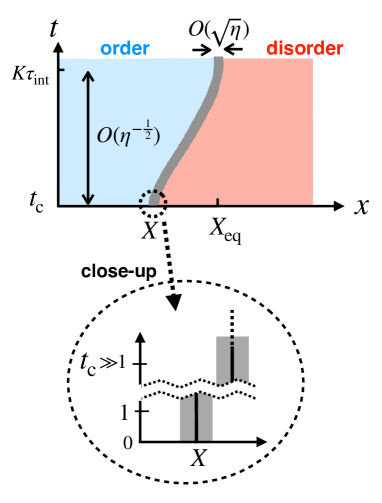
Figure 6: Space-time plot associated with interface motion whose time scale is $O(\eta^{-1/2})$. Its close-up at a time scale of $O(1)$ is also shown.

V Entropy production in the interface region

In this section, we estimate the entropy production in the interface region and obtain the final form of the stationary distribution for interface configurations. Concretely, in Sec. V.1, we explain a phenomenological method to obtain the temperature gap over the interface region. In Sec. V.2, we derive the temperature profile in the bulk when the interface slowly moves to the equilibrium position. By using this result, in Sec. V.3, we estimate the temperature gap at the interface. At last, in Sec. V.4, we show the result of ${\cal I}$ for a single interface configuration $\alpha_{X}$.

V.1 Phenomenological argument

Let us recall that the interface velocity $dX/dt$ would be determined by the free energy difference if the temperature of the system were uniform. See (D.14) in Appendix D. In the present problem, for a given small $dX/dt$, an inhomogeneous temperature profiles in the bulk regions are calculated, as shown in Sec. V.2. The average temperatures in the ordered and disordered regions are determined by two conditions. The first is clearly the energy conservation, while the second condition should be considered seriously. Since $\eta$ is finite, we consider the interface region as a thermodynamic subsystem. That is, the system consists of the three local equilibrium subsystems, corresponding to the ordered region, disordered region and the interface region, respectively. We then describe the energy exchange between each bulk region and the interface region. This description provides the second condition for determining the average temperatures for the given $dX/dt$. Macroscopic variables corresponding to the energy exchange are defined by

$$\Psi^{\rm o} \equiv \int_{0}^{X_{-}}dx\left(u^{\rm o}(T(x,t))-\frac{E}{A}\right),$$ (V.1)

$$\Psi^{\rm d} \equiv \int_{X_{+}}^{1}dx\left(u^{\rm d}(T(x,t))-\frac{E}{A}\right)$$ (V.2)

with (II.15) and (II.16) for the definition of $u^{\rm o}$ and $u^{\rm d}$. Note that $\Psi^{\rm o}(t)$ and $\Psi^{\rm d}(t)$ satisfy the energy conservation

$$\Psi^{\rm o}+\Psi^{\rm d}+\left(U^{\rm int}-\frac{E}{A}\Delta X\right)+O(\eta)=0,$$ (V.3)

where $\Delta X\equiv X_{+}-X_{-}$, $O(\eta)$ includes the term proportional to $(dX/dt)^{2}$, and $U^{\rm int}$ is the internal energy of the interface region, which includes the surface energy. Accordingly, the entropy of the system $S$ is expressed as

$$S=S^{\rm o}+S^{\rm d}+S^{\rm int},$$ (V.4)

where $S^{\rm o}$ and $S^{\rm d}$ are defined as

$$S^{\rm o}\equiv\int_{0}^{X_{-}}dxs^{\rm o}(T(x)),$$ (V.5)

$$S^{\rm d}\equiv\int_{X_{+}}^{1}dxs^{\rm d}(T(x)),$$ (V.6)

with (II.23) and (II.24), and $S^{\rm int}$ is assumed as a function of $U^{\rm int}$. Assuming that $\Psi^{\rm o}$ and $\Psi^{\rm d}$ are slow variables for the given interface motion $X(t)$, we write the Onsager form of their time evolution as

$$\frac{d\Psi^{\rm o}}{dt} = L^{\rm o}\left({\frac{\partial S}{\partial\Psi^{\rm o}}}\right)_{\Psi^{\rm d}},$$ (V.7)

$$\frac{d\Psi^{\rm d}}{dt} = L^{\rm d}\left({\frac{\partial S}{\partial\Psi^{\rm d}}}\right)_{\Psi^{\rm o}},$$ (V.8)

where ${L}^{\rm o}$ and ${L}^{\rm d}$ are new Onsager coefficients in this projected dynamics. Note that we do not take account of off-diagonal components of Onsager coefficients. See Fig. 7 for a schematic figure of the setup.

Since $\Psi^{\rm o/d}$ is related to $\beta_{-/+}^{\rm int}$ as shown in Sec. V.3, (V.7) and (V.8) give an expression of $\beta_{+}^{\rm int}-\beta_{-}^{\rm int}$ in terms of $X$, $dX/dt$, $\lambda^{\rm o/d}$, and ${L}^{\rm o/d}$. Here, fluctuations are renormalized into ${L}^{\rm o/d}$ so that ${L}^{\rm o/d}$ is determined by finite time fluctuations of the energy transfer into the ordered/disordered region from the interface. Moreover, we assume that fluctuations of $\Psi^{\rm o}$ and $\Psi^{\rm d}$ are not correlated, because the main contribution to the energy transfer comes from the latent heat generated at the interface. Therefore, ${L}^{\rm o/d}$ is given by quantities defined in the ordered/disordered region. Recalling that the dimension of ${L}^{\rm o/d}$ is that of $\lambda^{\rm o/d}$ divided by the length dimension, we set ${L}^{\rm o}$ and ${L}^{\rm d}$ as

$${L}^{\rm o} = \frac{\lambda^{\rm o}}{gX_{-}},$$ (V.9)

$${L}^{\rm d} = \frac{\lambda^{\rm d}}{g(1-X_{+})},$$ (V.10)

where $g$ is a dimensionless factor, which is assumed to be independent of $X$. When we impose the condition that the inverse temperature gap $\beta_{+}^{\rm int}-\beta_{-}^{\rm int}$ vanishes in the limit $X_{-}\to 0$ and $X_{+}\to 1$, we can determine the value of $g$ uniquely, as shown in the next section.

Precisely writing, (V.7) and (V.8) with (V.9) and (V.10) are not yet derived from the stochastic model we study. Rather, this description involves uncontrolled approximations. For example, the dynamics of $\Psi^{\rm o}$ may influence the interface motion and ${L}^{\rm o}$ may depend on $\lambda^{\rm d}$. We do not find clear reasons to ignore these effects. Nevertheless, we expect that (V.7) and (V.8) with (V.9) and (V.10) describe qualitative behaviors. In the subsequent subsections, we calculate the temperature profiles in the bulk regions and determine the temperature gap by explicitly expressing (V.7) and (V.8) in terms of $\beta_{+/-}^{\rm int}$.

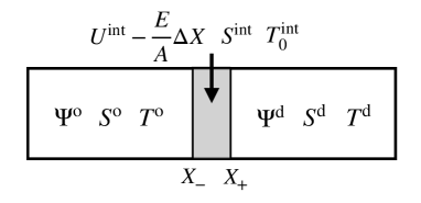
Figure 7: Coarse-grained description for determining the temperature gap at the interface. See (V.33) for $T_{0}^{\rm int}$.

V.2 Temperature profile in the bulk

In the bulk regions $[0,X_{-}(t)]$ and $[X_{+}(t),1]$ for the time interval $[t_{c},K\tau_{\rm int}]$, the time evolution is described by the deterministic equation. We ignore the terms associated with interface thermodynamics by setting $d_{e}=d_{f}=0$. We then study the behavior in the two bulk regions separately. Specifically, we study the entropy density $s(x,t)$. By substituting the thermodynamic relation

$$\partial_{t}s=\beta\partial_{t}u+\left({\frac{\partial s}{\partial m}}\right)_{u}\partial_{t}m$$ (V.11)

into (II.43), we obtain

$$T\partial_{t}s=\partial_{x}(\kappa\partial_{x}T)+\gamma(\partial_{t}m)^{2}.$$ (V.12)

In the ordered region $[0,X_{-}(t)]$, we may assume $m(x,t)=m_{\rm loc}(T(x,t))$, because $m(x,t)$ quickly relaxes to the local stable state for a given temperature $T(x,t)$. Then, since $s(x,t)=s^{\rm o}(T(x,t))$, we have

$$T\partial_{t}s = T\partial_{t}s^{\rm o}$$ (V.13)

$$= c^{\rm o}\partial_{t}T,$$ (V.14)

where we have used (II.25). By using this relation and noting $(\partial_{t}m)^{2}=O(\eta)$, we obtain

$$c^{\rm o}\partial_{t}T=\partial_{x}(\kappa\partial_{x}T)+O(\eta).$$ (V.15)

Let us recall $\kappa=\lambda/T^{2}$ and we set

$$\kappa_{X}^{\rm o}=\frac{\lambda^{\rm o}}{(T_{X}^{\rm qeq})^{2}}.$$ (V.16)

Since the time derivative of $T_{X(t)}^{\rm qeq}$ is given by

$$\frac{dT_{X(t)}^{\rm qeq}}{dt}=\left.\frac{dT_{X}^{\rm qeq}}{dX}\right|_{X=X(t)}\frac{dX}{dt}=O(\sqrt{\eta}),$$ (V.17)

the solution for small $\eta$ can be expanded as

$$T(x,t)=T^{(0)}(x,t)+\sqrt{\eta}T^{(1)}(x,t)+O(\eta).$$ (V.18)

By substituting (V.18) into (V.15), we first have

$$\partial_{x}T^{(0)}+O(\sqrt{\eta})=0$$ (V.19)

as the lowest order equation. The solution $T^{(0)}$ is constant in $x$. Since we study an interface configuration with the interface position $X$, the solution is the quasi-equilibrium profile

$$T^{(0)}(x,t)=T_{X(t)}^{\rm qeq},$$ (V.20)

which slowly evolves through the interface position $X(t)$. Next, by substituting

$$T(x,t)=T_{X(t)}^{\rm qeq}+\sqrt{\eta}T^{(1)}(x,t)+O(\eta)$$ (V.21)

into (V.15), we obtain

$$c^{\rm o}\frac{dT_{X}^{\rm qeq}}{dX}\frac{dX}{dt}=\sqrt{\eta}\kappa_{X}^{\rm o}\partial_{x}^{2}T^{(1)}+O(\eta),$$ (V.22)

where we have ignored $\sqrt{\eta}\partial_{t}T^{(1)}$ because this term is estimated as $O(\eta)$. Hereafter, $c^{\rm o}$ is evaluated at $T_{X(t)}^{\rm qeq}$. By solving this equation with the boundary condition $\partial_{x}T=0$ at $x=0$, we derive $T^{(1)}$ as a quadratic function in $x$. We thus obtain

$$T(x,t)={T^{\rm int}_{-}}(t)+\frac{dT_{X(t)}^{\rm qeq}}{dt}\frac{c^{\rm o}}{2\kappa_{X(t)}^{\rm o}}(x^{2}-X^{2})+O(\eta),$$ (V.23)

where $T_{-}^{\rm int}(t)=1/\beta_{-}^{\rm int}(t)$. Note that $T_{-}^{\rm int}(t)-T_{X(t)}^{\rm qeq}=O(\sqrt{\eta})$ should hold from (V.21).

Similarly, in the disordered region $x\in[X_{+}(t),1]$, we obtain

$$T(x,t)={T_{+}^{\rm int}}(t)+\frac{dT_{X(t)}^{\rm qeq}}{dt}\frac{c^{\rm d}}{2\kappa_{X(t)}^{\rm d}}[(1-x)^{2}-(1-X)^{2}]+O(\eta),$$ (V.24)

where $T_{+}^{\rm int}(t)=1/\beta_{+}^{\rm int}(t)$ and we have defined

$$\kappa_{X}^{\rm d}\equiv\frac{\lambda^{\rm d}}{(T_{X}^{\rm qeq})^{2}}.$$ (V.25)

In Fig. 8, we show a schematic figure of the temperature profiles in the two bulk regions. An important observation is that the temperature of the interface region is higher than that of the bulk regions when $dX/dt>0$. Physically, the slowly moving interface in the relaxation process produces the latent heat which acts as a heat source. This brings the distortion of the temperature profiles in the bulk regions. Note that $T^{\rm int}_{+}$ and $T^{\rm int}_{-}$ are not determined yet.

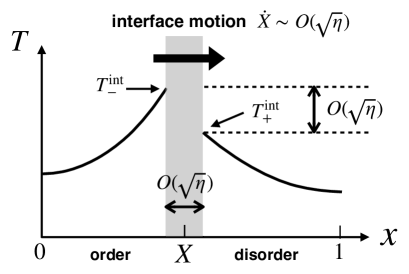
Figure 8: Temperature configuration in the late stage of a relaxation process. Latent heat is generated at the moving interface and it diffuses into the bulk regions. See (V.23) and (V.24) for the expression of the profiles. A temperature gap appears in the interface region. See (V.54) for the expression of the temperature gap.

V.3 Temperature gap

We define the average temperature in the ordered region as

$$T_{X}^{\rm o}(t)\equiv\frac{1}{X_{-}}\int_{0}^{X_{-}}dxT(x,t).$$ (V.26)

By substituting

$$u^{\rm o}(T(x,t))=u^{\rm o}(T_{X}^{\rm o})+c^{\rm o}(T(x,t)-T_{X}^{\rm o})+O(\eta)$$ (V.27)

into (V.1) and using (V.26), we obtain

$$\Psi^{\rm o}=\left(u^{\rm o}(T_{X}^{\rm o})-\frac{E}{A}\right)X_{-}+O(\eta).$$ (V.28)

Similarly, by using

$$T_{X}^{\rm d}(t)\equiv\frac{1}{1-X_{+}}\int_{X_{+}}^{1}dxT(x,t),$$ (V.29)

we have

$$\Psi^{\rm d}=\left(u^{\rm d}(T_{X}^{\rm d})-\frac{E}{A}\right)(1-X_{+})+O(\eta).$$ (V.30)

We also obtain

$$S^{\rm o} = X_{-}s^{\rm o}(T_{X}^{\rm o})+O(\eta),$$ (V.31)

$$S^{\rm d} = (1-X_{+})s^{\rm d}(T_{X}^{\rm d})+O(\eta).$$ (V.32)

We then define $T_{0}^{\rm int}$ as

$$T_{0}^{\rm int}\equiv\frac{dU^{\rm int}}{dS^{\rm int}},$$ (V.33)

which represents the temperature in the interface region.

We here apply the Onsager theory to two macroscopic quantities $\Psi^{\rm o}$ and $\Psi^{\rm d}$. We fix $\Psi^{\rm d}$ and consider the variation $\Psi^{\rm o}\to\Psi^{\rm o}+\delta\Psi^{\rm o}$. From energy conservation, we have

$$\delta\Psi^{\rm o}+\delta U^{\rm int}=0.$$ (V.34)

Since $\Psi^{\rm o}$ has the one-to-one correspondence with $T_{X}^{\rm o}$, as shown in (V.28), we have

$$\delta\Psi^{\rm o}=X_{-}c^{\rm o}\delta T_{X}^{\rm o}+O(\eta).$$ (V.35)

By using (V.34) and (V.35), we derive

$$\delta S = X_{-}\frac{c^{\rm o}}{T_{X}^{\rm o}}\delta T_{X}^{\rm o}+\frac{1}{T_{0}^{\rm int}}\delta U^{\rm int}$$ (V.36)

$$= \left(\frac{1}{T_{X}^{\rm o}}-\frac{1}{T_{0}^{\rm int}}\right)\delta\Psi^{\rm o}.$$

Therefore, the equation of $\Psi^{\rm o}$ in (V.7) is written as

$$\frac{d\Psi^{\rm o}}{dt}={L}^{\rm o}\left(\frac{1}{T_{X}^{\rm o}}-\frac{1}{T_{0}^{\rm int}}\right).$$ (V.37)

Similarly, (V.8) becomes

$$\frac{d\Psi^{\rm d}}{dt}={L}^{\rm d}\left(\frac{1}{T_{X}^{\rm d}}-\frac{1}{T_{0}^{\rm int}}\right).$$ (V.38)

From (V.37) and (V.38), we obtain

$$\frac{1}{T_{X}^{\rm d}}-\frac{1}{T_{X}^{\rm o}}=\frac{1}{{L}^{\rm d}}\frac{d\Psi^{\rm d}}{dt}-\frac{1}{{L}^{\rm o}}\frac{d\Psi^{\rm o}}{dt}.$$ (V.39)

Let us express $T_{X}^{\rm o/d}$ in terms of $T_{+/-}^{\rm int}$. By using (V.23), we calculate

$$T_{X}^{\rm o}=T_{-}^{\rm int}-\frac{dT_{X}^{\rm qeq}}{dt}\frac{c^{\rm o}(T_{X}^{\rm qeq})^{2}}{3\lambda^{\rm o}}X^{2}+O(\eta).$$ (V.40)

Similarly, we have

$$T_{X}^{\rm d}=T_{+}^{\rm int}-\frac{dT_{X}^{\rm qeq}}{dt}\frac{c^{\rm d}(T_{X}^{\rm qeq})^{2}}{3\lambda^{\rm d}}(1-X)^{2}+O(\eta).$$ (V.41)

Hereafter, we do not explicitly write $O(\eta)$. From (V.40) and (V.41), we obtain

$$\frac{1}{T_{X}^{\rm d}}-\frac{1}{T_{X}^{\rm o}}= \beta_{+}^{\rm int}-\beta_{-}^{\rm int}$$

$$+\frac{dT_{X}^{\rm qeq}}{dt}\left[\frac{c^{\rm d}}{3\lambda^{\rm d}}(1-X)^{2}-\frac{c^{\rm o}}{3\lambda^{\rm o}}X^{2}\right].$$ (V.42)

Substituting (V.42) into (V.39), we have

$$\beta_{+}^{\rm int}-\beta_{-}^{\rm int}= \frac{dT_{X}^{\rm qeq}}{dt}\left[\frac{c^{\rm o}}{3\lambda^{\rm o}}X^{2}-\frac{c^{\rm d}}{3\lambda^{\rm d}}(1-X)^{2}\right]$$

$$+\frac{1}{{L}^{\rm d}}\frac{d\Psi^{\rm d}}{dt}-\frac{1}{{L}^{\rm o}}\frac{d\Psi^{\rm o}}{dt}.$$ (V.43)

Next, we consider $d\Psi^{\rm o}/dt$. From (V.1), we calculate

$$\frac{d\Psi^{\rm o}}{dt}=\left(u^{\rm o}(T_{X}^{\rm qeq})-\frac{E}{A}\right)\frac{dX}{dt}+c^{\rm o}X\frac{dT_{X}^{\rm qeq}}{dt}.$$ (V.44)

Here, by using $u^{\rm o}(T)$ defined by (II.15), we have the following identity:

$$\frac{d}{dt}\left[X^{2}\left(u^{\rm o}(T_{X}^{\rm qeq})-\frac{E}{A}\right)\right]$$

$$=2X\frac{dX}{dt}\left(u^{\rm o}(T_{X}^{\rm qeq})-\frac{E}{A}\right)+X^{2}c^{\rm o}\frac{dT_{X}^{\rm qeq}}{dt}.$$ (V.45)

We also obtain

$$\psi_{X}^{\rm qeq}(X)=X\left(u^{\rm o}(T_{X}^{\rm qeq})-\frac{E}{A}\right),$$ (V.46)

from (IV.42). By using (V.9) and (V.45) with (V.46), we rewrite (V.44) as

$$\frac{1}{{L}^{\rm o}}\frac{d\Psi^{\rm o}}{dt}= \frac{g}{\lambda^{\rm o}}\left\{-\frac{dX}{dt}\psi_{X}^{\rm qeq}(X)+\frac{d}{dt}\left[X\psi_{X}^{\rm qeq}(X)\right]\right\}$$

$$= \frac{g}{\lambda^{\rm o}}\left(X\frac{d}{dt}\psi_{X}^{\rm qeq}(X)\right),$$ (V.47)

and we also have

$$\frac{dT_{X}^{\rm qeq}}{dt}\frac{c^{\rm o}}{3\lambda^{\rm o}}X^{2}=-\frac{1}{3\lambda^{\rm o}}\frac{dX}{dt}\psi_{X}^{\rm qeq}(X)+\frac{1}{3}\left[\frac{X}{\lambda^{\rm o}}\frac{d}{dt}\psi_{X}^{\rm qeq}(X)\right],$$ (V.48)

where we have replaced $X_{+/-}$ in (V.9) and (V.10) by $X$ with ignoring $O(\eta)$ terms.

Here, from (IV.43), we have

$$\left(u^{\rm d}(T_{X}^{\rm qeq})-\frac{E}{A}\right)(1-X)=-\psi_{X}^{\rm qeq}(X).$$ (V.49)

By using an identity similar to (V.45) and (V.49), we also have

$$\frac{1}{{L}^{\rm d}}\frac{d\Psi^{\rm d}}{dt}=-\frac{g}{\lambda^{\rm d}}\left((1-X)\frac{d}{dt}\psi_{X}^{\rm qeq}(X)\right),$$ (V.50)

and

$$\frac{dT_{X}^{\rm qeq}}{dt}\frac{c^{\rm d}}{3\lambda^{\rm d}}(1-X)^{2}= -\frac{1}{3\lambda^{\rm d}}\frac{dX}{dt}\psi_{X}^{\rm qeq}(X)$$

$$-\frac{1}{3}\left[\frac{1-X}{\lambda^{\rm d}}\frac{d}{dt}\psi_{X}^{\rm qeq}(X)\right].$$ (V.51)

By substituting (V.47), (V.48), (V.50) and (V.51) into (V.43), we obtain

$$\beta_{+}^{\rm int}-\beta_{-}^{\rm int}$$

$$=-\frac{1}{3}\left(\frac{1}{\lambda^{\rm o}}-\frac{1}{\lambda^{\rm d}}\right)\frac{dX}{dt}\psi_{X}^{\rm qeq}(X)$$

$$\quad-\left(g-\frac{1}{3}\right)\left(\frac{X}{\lambda^{\rm o}}+\frac{1-X}{\lambda^{\rm d}}\right)\frac{d}{dt}\left[\psi_{X}^{\rm qeq}(X)\right],$$ (V.52)

The formula (V.52) gives the inverse temperature gap of $O(\sqrt{\eta})$.

Let us recall that $g$ is a phenomenological parameter and its value is not specified yet. Here, we impose the condition that the temperature gap vanishes when $X\to 0$ and $X\to 1$. Noting that $dX/dt\not=0$ in the limit $X\to 0$ or $X\to 1$, this condition determines the unique value of $g$ as $g=1/3$. We then have arrived at the formula of the inverse temperature gap:

$$\beta_{+}^{\rm int}-\beta_{-}^{\rm int}=-\frac{1}{3}\left(\frac{1}{\lambda^{\rm o}}-\frac{1}{\lambda^{\rm d}}\right)\frac{dX}{dt}\psi_{X}^{\rm qeq}(X)$$ (V.53)

up to the error of $O(\eta)$. By using (IV.45), we can express (V.53) as

$$\beta_{+}^{\rm int}-\beta_{-}^{\rm int}=\frac{1}{3}\left(\frac{1}{\lambda^{\rm o}}-\frac{1}{\lambda^{\rm d}}\right)\frac{dX}{dt}X(1-X)q_{X}.$$ (V.54)

This formula clearly indicates that the temperature gap is associated with the latent heat generated at the moving interface. See Fig. 8 for the summary of the result.

V.4 Final result

We substitute (V.53) into (IV.52). We then obtain

$$\lim_{K\to\infty}\lim_{\eta\to 0}I_{2}^{\rm int}(\alpha_{X})=-\frac{1}{3}\int_{X}^{X_{\rm eq}}\!\!\!\!dY\psi_{Y}^{\rm qeq}(Y)\left(\frac{1}{\lambda^{\rm o}}-\frac{1}{\lambda^{\rm d}}\right).$$ (V.55)

By combining (IV.47) and (V.55) in the formula (IV.21), we complete the calculation of the correction term as

$${\cal I}(\alpha_{X}) = \frac{A}{\lambda^{\rm o}}\int_{0}^{X}dx\psi_{X}(x)+\frac{A}{\lambda^{\rm d}}\int_{X}^{1}dx\psi_{X}(x)$$ (V.56)

$$-\frac{A}{\lambda^{\rm o}}\int_{0}^{X_{\rm eq}}dx\psi_{X_{\rm eq}}^{\rm qeq}(x)-\frac{A}{\lambda^{\rm d}}\int_{X_{\rm eq}}^{1}dx\psi_{X_{\rm eq}}^{\rm qeq}(x)$$

$$+\frac{2A}{3}\int_{X}^{X_{\rm eq}}dY\psi_{Y}^{\rm qeq}(Y)\left(\frac{1}{\lambda^{\rm o}}-\frac{1}{\lambda^{\rm d}}\right).$$

By substituting (V.56) into (IV.8), we obtain

$$\tilde{\cal S}(\alpha_{X}; E,J)=A\int_{0}^{1}dxs(u_{X}(x),m_{X}(x))$$

$$+\frac{AJ}{\lambda^{\rm o}}\int_{0}^{X}dx\psi_{X}(x)+\frac{AJ}{\lambda^{\rm d}}\int_{X}^{1}dx\psi_{X}(x)$$

$$-\frac{2AJ}{3}\int^{X}_{0}dY\psi_{Y}^{\rm qeq}(Y)\left(\frac{1}{\lambda^{\rm o}}-\frac{1}{\lambda^{\rm d}}\right)$$ (V.57)

up to an additive constant independent of $X$. Combining it with (IV.7), we finally obtain the stationary distribution of interface configurations.

VI Variational principle

We consider the case $E_{1}\leq E\leq E_{2}$ with (II.13) and (II.14). When $J=0$, the most probable configuration contains a single interface, whose position is determined by the microcanonical ensemble. Explicitly, the position $X_{*}$ maximizes the total entropy. Even when $J\not=0$, the most probable configuration may contain a single interface. We then expect that its position $X_{*}$ is determined by a variational principle that is obtained as an extension of the maximum entropy principle when $\epsilon=|J|$ is small. In this section, we study this variational principle. In Sec. VI.1, we present a formulation of the problem. In Sec. VI.2, we explicitly derive the variational function. After some preliminaries in Sec. VI.3, we re-express the variational equation as the form of the free energy difference at the interface in Sec. VI.4. In Sec. VI.5, from this expression, we derive the temperature of the interface. Throughout this section, we evaluate quantities neglecting $O(\epsilon^{2})$ terms even without explicit remarks.

VI.1 Formulation of the problem

We assume that the most probable profile in the steady state is independent of $(y,z)$ and possesses an interface at $x=X_{*}$. Then, we observe the ordered state in the region $0\leq x<X_{*}$ and the disordered state in the region $X_{*}<x\leq 1$. When $X_{*}$ is given, the most probable profile of $(m({\boldsymbol{r}}),v({\boldsymbol{r}}),\phi({\boldsymbol{r}}))$ in the limit $\eta\to 0$ is determined from the conditions $v({\boldsymbol{r}})=0$, $\sigma(T,m)=0$, and $\lambda\partial_{x}\beta=J$ in each region. It should be noted that $X_{*}$ is not obtained by the stationary solution of (II.65), (II.66), and (II.67) with $\eta=0$. Thus, we determine $X_{*}$ by considering the probability density $P(X;E,J)$ of the interface position $X$ for small $\eta$. We expect that $P(X;E,J)$ takes the form

$$P(X;E,J)=e^{\frac{1}{\eta^{3}}\left[{\cal V}(X;E,J)+O(\sqrt{\eta})\right]}$$ (VI.1)

in the limit $\eta\to 0$. Here, the potential function ${\cal V}(X)$ is independent of $\eta$. Then, the most probable position of the interface $X_{*}$ is given as the maximizer of ${\cal V}(X;E,J)$, which is the variational principle we expect.

We consider the potential function ${\cal V}(X)$. For equilibrium cases $J=0$, ${\cal V}(X)$ is given as the total entropy for the quasi-equilibrium profile with the interface position $X$ in the limit $\eta\to 0$. We generalize this result to the case $J<0$.

Let ${\cal C}_{X}$ be the set of configurations with a single interface with the interface position $X$. Suppose that a configuration with a single interface is observed. The probability density of the interface position $X$ on this condition is expressed as

$$P(X;E,J)=\frac{\int_{{\cal C}_{X}}d\alpha_{X}{\cal P}_{\rm ss}(\alpha_{X};E,J)}{\int_{0}^{1}dY\int_{{\cal C}_{Y}}d\alpha_{Y}{\cal P}_{\rm ss}(\alpha_{Y};E,J)},$$ (VI.2)

where ${\cal P}_{\rm ss}$ is given by (IV.7). Since we consider the limit $\eta\to 0$, we reasonably conjecture from (VI.1) that

$${\cal V}(X;E,J)=\max_{\alpha_{X}\in{\cal C}_{X}}\tilde{\cal S}(\alpha_{X};E,J),$$ (VI.3)

where fluctuations of $\alpha_{X}$ are assumed to be sub-leading in the evaluation of ${\cal V}(X;E,J)$.

VI.2 Formula of the potential

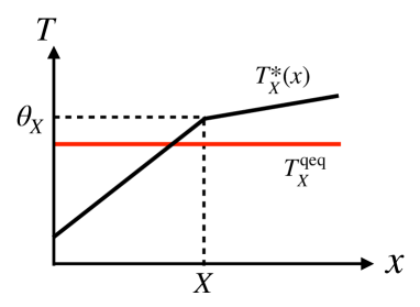
Figure 9: Temperature profile $T_{X}^{*}(x)$ that maximizes the modified entropy $\tilde{\cal S}(\alpha_{X};E,J)$ for a given $X$. $\kappa^{\rm d}>\kappa^{\rm o}$.

We calculate the right-hand side of (VI.3). Note that the last line of (V.57) is independent of $\alpha_{X}$, while it depends on $X$. Thus, the last line is not relevant in the maximization of $\tilde{\cal S}(\alpha_{X};E,J)$, but necessary in the maximization of ${\cal V}(X;E,J)$ in $X$. Let $\alpha_{X}^{*}$ be the maximizer of $\tilde{\cal S}(\alpha_{X};E,J)$ with $X$ fixed. We then rewrite (VI.3) as

$${\cal V}(X;E,J)=\tilde{\cal S}(\alpha_{X}^{*};E,J).$$ (VI.4)

Now, we derive $\alpha_{X}^{*}$ by taking the variation of $\tilde{\cal S}(\alpha_{X};E,J)$ in $m_{X}$, $v_{X}$ and $\psi_{X}$. The result of the variation

$$\int_{0}^{1}dx\left[(\delta\psi_{X})\left(-\partial_{x}\beta_{X}+\frac{J}{\lambda}\right)\right.$$

$$+\left.(\delta m_{X})\beta\sigma(u_{X},m_{X})-(\delta v_{X})\beta v_{X}\right]=0$$ (VI.5)

leads to

$$J=\lambda^{\rm o}\partial_{x}\beta^{*}_{X}\qquad{\rm for}\quad x<X,$$ (VI.6)

$$J=\lambda^{\rm d}\partial_{x}\beta^{*}_{X}\qquad{\rm for}\quad x>X,$$ (VI.7)

$$\sigma(T^{*}_{X}(x),m^{*}_{X}(x))=0,$$ (VI.8)

$$v_{X}^{*}(x)=0,$$ (VI.9)

where note that $\psi_{X}^{\rm qeq}(x)$ is independent of $\alpha_{X}$. Here, let $\theta$ be an interface temperature. For given $X$ and $\theta$, we define a new quantity $\tilde{T}^{*}_{X}(x;\theta)$ as the solution of (VI.6) and (VI.7) with $\tilde{T}_{X}^{*}(X;\theta)=\theta$. Obviously, $\tilde{T}^{*}_{X}(x;\theta)$ is equivalent to the stationary solution of the transportation equation in the heat conduction. Then, energy conservation

$$A\int_{0}^{1}dxu(\tilde{T}^{*}_{X}(x;\theta),m^{*}_{X}(x))=E$$ (VI.10)

provides the special value of $\theta$, which is denoted by $\theta_{X}$. $T_{X}^{*}(x)$ is determined by $T_{X}^{*}(x)=\tilde{T}^{*}_{X}(x;\theta_{X})$, and then $m^{*}_{X}(x)$ is determined from (VI.8). In Fig. 9, we display an example of the temperature profile $T_{X}^{*}(x)$. Since $T_{X}^{*}(x)=T_{X}^{\rm qeq}+O(\epsilon)$, we also have

$$\psi_{X}^{*}(x) = \int_{0}^{x}dy\left[u^{\rm o}(T_{X}^{*}(y))-\frac{E}{A}\right]$$ (VI.11)

$$= \psi_{X}^{\rm qeq}(x)+O(\epsilon)$$

for $x<X$. Similarly,

$$\psi_{X}^{*}(x)=\psi_{X}^{\rm qeq}(x)+O(\epsilon)$$ (VI.12)

for $x>X$. By substituting these results into (VI.4) with(V.57) , we obtain

$${\cal V}(X;E,J)$$

$$=A\int_{0}^{X}dxs^{\rm o}(T^{*}_{X}(x))+A\int_{X}^{1}dxs^{\rm d}(T^{*}_{X}(x))$$

$$\quad+\frac{AJ}{\lambda^{\rm o}}\int_{0}^{X}dx\psi_{X}^{\rm qeq}(x)+\frac{AJ}{\lambda^{\rm d}}\int_{X}^{1}dx\psi_{X}^{\rm qeq}(x)$$

$$\quad-\frac{2AJ}{3}\int^{X}_{0}dY\psi_{Y}^{\rm qeq}(Y)\left(\frac{1}{\lambda^{\rm o}}-\frac{1}{\lambda^{\rm d}}\right).$$ (VI.13)

Then, (VI.10) is written as

$$A\int_{0}^{X}dxu^{\rm o}(T^{*}_{X}(x))+A\int_{X}^{1}dxu^{\rm d}(T^{*}_{X}(x))=E.$$ (VI.14)

VI.3 Preliminaries for maximization of the potential

In order to calculate $X_{*}$ that maximizes ${\cal V}(X)$ under the condition (VI.14), we present some preliminaries. First, noting

$$\partial_{x}s_{X}^{*}(x)=-T^{*}_{X}c^{\rm o}(T^{*}_{X})\frac{J}{\lambda^{\rm o}}$$ (VI.15)

for $x<X$, we obtain

$$s_{X}^{*}(x) = s^{\rm o}(\theta_{X})-\int_{X}^{x}dxT^{*}_{X}(x)c^{\rm o}(T^{*}_{X})\frac{J}{\lambda^{\rm o}}$$ (VI.16)

$$= s^{\rm o}(\theta_{X})-(x-X)\theta_{X}c^{\rm o}(\theta_{X})\frac{J}{\lambda^{\rm o}},$$

which leads to

$$\int_{0}^{X}dxs_{X}^{*}(x) = Xs^{\rm o}(\theta_{X})+\frac{X^{2}}{2}\theta_{X}c^{\rm o}(\theta_{X})\frac{J}{\lambda^{\rm o}}$$ (VI.17)

$$= Xs^{\rm o}\left(\theta_{X}+\theta_{X}^{2}\frac{XJ}{2\lambda^{\rm o}}\right).$$

Similarly, we have

$$\int_{X}^{1}dxs_{X}^{*}(x)=(1-X)s^{\rm d}\left(\theta_{X}-\theta_{X}^{2}\frac{(1-X)J}{2\lambda^{\rm d}}\right).$$ (VI.18)

Here, it is convenient to introduce

$$T_{X}^{\rm o} = \theta_{X}+\theta_{X}^{2}\frac{XJ}{2\lambda^{\rm o}},$$ (VI.19)

$$T_{X}^{\rm d} = \theta_{X}-\theta_{X}^{2}\frac{(1-X)J}{2\lambda^{\rm d}}.$$ (VI.20)

It should be noted that

$$T_{X}^{\rm o} = \frac{1}{X}\int_{0}^{X}dxT_{X}^{*}(x)+O(\epsilon^{2}),$$ (VI.21)

$$T_{X}^{\rm d} = \frac{1}{1-X}\int_{X}^{1}dxT_{X}^{*}(x)+O(\epsilon^{2}).$$ (VI.22)

That is, $T_{X}^{\rm o}$ and $T_{X}^{\rm d}$ are the spatially averaged temperatures in the ordered phase and in the disordered phase, respectively, which are basically the same as those in (V.26) and (V.29).

VI.4 Variational equation

In this subsection, we simplify the variational equation. Substituting (IV.42) and (IV.43) into (VI.13), we have

$$\frac{{\cal V}(X;E,J)}{A}=Xs^{\rm o}(T_{X}^{\rm o})+(1-X)s^{\rm d}(T_{X}^{\rm d})$$

$$\quad+\frac{X^{2}J}{2\lambda^{\rm o}}\left(u^{\rm o}(\theta_{X})-\frac{E}{A}\right)-\frac{(1-X)^{2}J}{2\lambda^{\rm d}}\left(u^{\rm d}(\theta_{X})-\frac{E}{A}\right)$$

$$\quad-\frac{2J}{3}\left(\frac{1}{\lambda^{\rm o}}-\frac{1}{\lambda^{\rm d}}\right)\int^{X}_{0}dY\left(u^{\rm o}(\theta_{Y})-\frac{E}{A}\right)Y,$$ (VI.23)

where $\theta_{X}$ in the right hand side is a function of $X$ whose dependence is determined by

$$Xu^{\rm o}(T_{X}^{\rm o})+(1-X)u^{\rm d}(T_{X}^{\rm d})=\frac{E}{A},$$ (VI.24)

where $T_{X}^{\rm o}$ and $T_{X}^{\rm d}$ are given by (VI.21) and (VI.22).

Then, the variational equation

$$\frac{d\cal V}{dX}=0$$ (VI.25)

becomes

$$s^{\rm o}(T_{X}^{\rm o})-s^{\rm d}(T_{X}^{\rm d})$$

$$+X\frac{c^{\rm o}(T_{X}^{\rm o})}{T_{X}^{\rm o}}\frac{dT_{X}^{\rm o}}{dX}+(1-X)\frac{c^{\rm d}(T_{X}^{\rm d})}{T_{X}^{\rm d}}\frac{dT_{X}^{\rm d}}{dX}$$

$$+\frac{XJ}{\lambda^{\rm o}}\left(u^{\rm o}(\theta_{X})-\frac{E}{A}\right)+\frac{(1-X)J}{\lambda^{\rm d}}\left(u^{\rm d}(\theta_{X})-\frac{E}{A}\right)$$

$$+\left[\frac{X^{2}J}{2\lambda^{\rm o}}c^{\rm o}(\theta_{X})-\frac{(1-X)^{2}J}{2\lambda^{\rm d}}c^{\rm d}(\theta_{X})\right]\frac{d\theta_{X}}{dX}$$

$$-\frac{2J}{3}\left(\frac{1}{\lambda^{\rm o}}-\frac{1}{\lambda^{\rm d}}\right)\left(u^{\rm o}(\theta_{X})-\frac{E}{A}\right)X$$

$$=0.$$ (VI.26)

From (VI.24), we also obtain

$$u^{\rm o}(T_{X}^{\rm o})-u^{\rm d}(T_{X}^{\rm d})+Xc^{\rm o}(T_{X}^{\rm o})\frac{dT_{X}^{\rm o}}{dX}+(1-X)c^{\rm d}(T_{X}^{\rm d})\frac{dT_{X}^{\rm d}}{dX}=0.$$ (VI.27)

The second line of (VI.26) is expressed as

$$X\frac{c^{\rm o}(T_{X}^{\rm o})}{\theta_{X}}\frac{dT_{X}^{\rm o}}{dX}+(1-X)\frac{c^{\rm d}(T_{X}^{\rm d})}{\theta_{X}}\frac{dT_{X}^{\rm d}}{dX}$$

$$+X(\theta_{X}-T_{X}^{\rm o})\frac{c^{\rm o}(T_{X}^{\rm o})}{\theta_{X}^{2}}\frac{dT_{X}^{\rm o}}{dX}$$

$$+(1-X)(\theta_{X}-T_{X}^{\rm d})\frac{c^{\rm d}(T_{X}^{\rm d})}{\theta_{X}^{2}}\frac{dT_{X}^{\rm d}}{dX}.$$ (VI.28)

By using (VI.27), we find that the first line in (VI.28) is

$$-\frac{u^{\rm o}(T_{X}^{\rm o})-u^{\rm d}(T_{X}^{\rm d})}{\theta_{X}}.$$ (VI.29)

The combination with the first line in (VI.26) yields

$$s^{\rm o}(T_{X}^{\rm o})-\frac{u^{\rm o}(T_{X}^{\rm o})}{\theta_{X}}-\left[s^{\rm d}(T_{X}^{\rm d})-\frac{u^{\rm d}(T_{X}^{\rm d})}{\theta_{X}}\right]$$

$$=s^{\rm o}(\theta_{X})-\frac{u^{\rm o}(\theta_{X})}{\theta_{X}}-\left[s^{\rm d}(\theta_{X})-\frac{u^{\rm o}(\theta_{X})}{\theta_{X}}\right]$$

$$=-\frac{f^{\rm o}(\theta_{X})-f^{\rm d}(\theta_{X})}{\theta_{X}},$$ (VI.30)

where we have defined

$$f^{\rm o}(\theta_{X}) = u^{\rm o}(\theta_{X})-\theta_{X}s^{\rm o}(\theta_{X}),$$ (VI.31)

$$f^{\rm d}(\theta_{X}) = u^{\rm o}(\theta_{X})-\theta_{X}s^{\rm d}(\theta_{X}).$$ (VI.32)

The second and third lines in (VI.28) become

$$-\frac{X^{2}J}{2\lambda^{\rm o}}c^{\rm o}(T_{X}^{\rm o})\frac{dT_{X}^{\rm o}}{dX}+\frac{(1-X)^{2}J}{2\lambda^{\rm d}}{c^{\rm d}(T_{X}^{\rm d})}\frac{dT_{X}^{\rm d}}{dX},$$ (VI.33)

which cancels with the forth line in (VI.26). The third line and the fifth line in (VI.26) are summarized as

$$\frac{J}{3}\left(\frac{1}{\lambda^{\rm o}}-\frac{1}{\lambda^{\rm d}}\right)\left(u^{\rm o}(\theta_{X})-\frac{E}{A}\right)X,$$ (VI.34)

where we have used

$$X\left(u^{\rm o}(\theta_{X})-\frac{E}{A}\right)+(1-X)\left(u^{\rm d}(\theta_{X})-\frac{E}{A}\right)=O(\epsilon),$$ (VI.35)

which comes from (VI.24). Furthermore, noting (IV.45), we re-express (VI.34) as

$$-\frac{J}{3}\left(\frac{1}{\lambda^{\rm o}}-\frac{1}{\lambda^{\rm d}}\right){X(1-X)}q_{X}.$$ (VI.36)

In this manner, (VI.30) and (VI.36) remain in the left-hand side of (VI.26). Thus, the variational equation (VI.26) is simplified as

$$f^{\rm o}(\theta_{X})-f^{\rm d}(\theta_{X})=-\frac{\theta_{X}J}{3}\left(\frac{1}{\lambda^{\rm o}}-\frac{1}{\lambda^{\rm d}}\right){X(1-X)}q_{X}.$$ (VI.37)

This equation with (VI.24) gives the most probable value $(\theta_{*},X_{*})$ of the interface temperature $\theta$ and the interface position $X$.

VI.5 Result

When we set $J=0$ in (VI.24) and (VI.37), we find that $\theta_{*}=T_{c}(=1)$ and $X_{*}=X_{\rm eq}$ given by (III.3). When $J\not=0$, we derive the equation for $\theta_{*}-T_{c}$ from (VI.37) as

$$-(s^{\rm o}(T_{c})-s^{\rm d}(T_{c}))(\theta_{*}-T_{c})$$

$$\quad=-\frac{T_{c}J}{3}\left(\frac{1}{\lambda^{\rm o}}-\frac{1}{\lambda^{\rm d}}\right){X_{\rm eq}(1-X_{\rm eq})}q_{X},$$ (VI.38)

which yields

$$\theta_{*}-T_{c}=-\frac{T_{c}^{2}J}{3}\left(\frac{1}{\lambda^{\rm o}}-\frac{1}{\lambda^{\rm d}}\right){X_{\rm eq}(1-X_{\rm eq})}.$$ (VI.39)

When we use the standard thermal conductivity $\kappa$ defined by (II.34), we rewrite (VI.39) as

$$\theta_{*}-T_{c}=-\frac{J}{3}\left(\frac{1}{\kappa^{\rm o}}-\frac{1}{\kappa^{\rm d}}\right){X_{\rm eq}(1-X_{\rm eq})}.$$ (VI.40)

Suppose that $\kappa^{\rm d}>\kappa^{\rm o}$ (or $\kappa^{\rm d}<\kappa^{\rm o}$). Noting $J<0$, we find $\theta_{*}>T_{c}$ (or $\theta_{*}<T_{c}$). This means that the super-heated ordered state (or super-cooled disordered state) stably appears near the interface in the heat conduction state. See Fig. 10. This phenomenon was predicted by an extended framework of thermodynamics NS , which is called global thermodynamics NS2 . If the factor $1/3$ were $1/2$, the result (VI.40) would be equivalent to the quantitative prediction by global thermodynamics. We conjecture that the discrepancy comes from the approximation we used in Sec. V.1. By comparing (VI.40) with (V.54), we find that $\theta_{*}-T_{c}$ is quantitatively connected to the temperature gap $T_{+}^{\rm int}-T_{-}^{\rm int}$ when $J$ is identified with $q_{X}dX/dt$.

Finally, from the left-right symmetry, we notice that $\theta_{*}$ is invariant for $(J,X)\to(-J,1-X)$. Thus, we express (VI.40) as

$$\theta_{*}-T_{c}=\frac{|J|}{3}\left(\frac{1}{\kappa^{\rm o}}-\frac{1}{\kappa^{\rm d}}\right){X_{\rm eq}(1-X_{\rm eq})}$$ (VI.41)

for any $J$. Note that the symmetry breaking field $\sigma^{\rm ex}(x)$ is also replaced by $\sigma^{\rm ex}(1-x)$ for the case $J>0$.

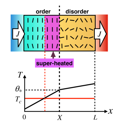
Figure 10: Schematic of the main result.

VII Concluding remarks

We have proposed the stochastic model (II.65), (II.66), and (II.67) for describing phase coexistence in heat conduction. As a special boundary condition, we imposed the non-equilibrium adiabatic condition (II.73) and (II.74) , which is a natural extension of the adiabatic condition with $J=0$. For this system, we formulated the variational principle for determining the interface position $X$. We have shown that the variational function ${\cal V}(X)$ given in (VI.3) is calculated as (VI.23). By solving the variational problem, we found that the interface temperature deviates from $T_{c}$, which implies that quasi-equilibrium states stably appear near the interface. Before ending this paper, we discuss possible directions for studies.

First, we consider a liquid-gas transition, which is the most popular first-order transition. The generalized hydrodynamics with the interface thermodynamics was proposed Anderson98 ; Bedeaux03 ; Onuki , and the fluctuating hydrodynamics without interfaces is well-established Schmitz . Thus, a stochastic model could be constructed through a combination of the two models. By imposing the non-equilibrium adiabatic boundary conditions, we may derive a potential function for determining the liquid-gas interface. It is reasonable to conjecture that the potential function is calculated from the modified entropy for the stationary profile of the interface position $X$, because the method developed in this paper can be used for liquid-gas coexistence in heat conduction. The main difference is that the density is conserved, which causes an additional contribution to the interface temperature, as shown in Ref. NS2 . Explicit calculation of the interface temperature may be an important exercise.

Secondly, the variational formula we have derived in this paper may be related to global thermodynamics for heat conduction NS2 . Both formulas predict that the interface temperature deviates from the transition temperature at equilibrium. To find the direct connection between the two theories, one may construct a thermodynamic framework by employing an extended Clausius relation for the stochastic order parameter dynamics. See Refs. Hatano-Sasa ; KNST ; NN ; Jona-thermo ; Maes-thermo ; Chiba-Nakagawa for studies related to an extended Clausius relation. This is the next subject in developing the theory.

Here, we briefly review the global thermodynamics. The theory describes spatially inhomogeneous systems by a few global quantities, such as the global temperature, which is defined such that the fundamental relation in thermodynamics is satisfied. This idea is simple and natural but has never been considered in previous studies seeking an extended framework of thermodynamics Keizer ; Eu ; Jou ; Oono-paniconi ; Sasa-Tasaki ; Bertin ; Seifert-contact ; Dickman . More importantly, this framework naturally leads to a quantitative prediction of the interface temperature $\theta$ different from $T_{c}$. Therefore, experiments can judge the validity of the fundamental hypothesis on which global thermodynamics is built. See Ref. NS2 for an explanation of the theory, including a comparison with other extended frameworks of thermodynamics.

Thirdly, the result on the interface temperature is obtained only for the special boundary condition. Naturally, one may want to derive the interface temperature for more standard cases where two heat baths of different temperatures contact with the system. Even for this case, we can use the stochastic dynamics (II.65), (II.66), and (II.67) with the boundary conditions $T(0,t)=T_{\rm L}$ and $T(1,t)=T_{\rm R}$. We can derive the Zubarev-Mclennan representation, which includes the time integration of the entropy production rate. This term can hardly be evaluated theoretically without knowing the steady state profile. Although we physically conjecture that the interface temperature is independent of boundary conditions when the value of the heat flux is the same, we do not have a proof of this conjecture. It is challenging to calculate the interface temperature for the boundary conditions $T(0,t)=T_{\rm L}$ and $T(1,t)=T_{\rm R}$.

Fourthly, to the best of our knowledge, the first-order transition in heat conduction has never been studied by systematic numerical experiments. One reason for this is that there are no paradigmatic models for describing the phase coexistence in heat conduction. It may be useful if such a numerical model was devised. Furthermore, by performing numerical simulations of such models, one may obtain a phase diagram of the system. In particular, the numerical determination of the interface temperature may be stimulating. The results will be compared with our theoretical results quantitatively.

Fifthly, related to the fourth problem, one may recall that the molecular dynamics simulations were performed in order to study the phase coexistence in heat conduction Bedeaux00 ; Ogushi . However, no deviation of the interface temperature from the transition temperature was observed. We conjecture that this is due to insufficient separation of scales. For example, when $\eta=10^{-2}$, the dimensionless interface width in our description is $10^{-1}$. Such a system may be well described by a deterministic equation, and thus $\theta=T_{c}$ holds. Even for such small systems, the precise measurement of fluctuating quantities may reveal the true behavior in the limit $\eta\to 0$. Formulating such statistical properties is an important theoretical problem.

Finally, the most important future study is to stably observe the super-heated ordered (or super-cooled disordered) state in laboratory experiments. Even qualitative observation of the stabilization of such states is quite interesting. To observe this phenomenon, a precise temperature profile should be measured. A novel concept must be designed for such an experimental setup.

After studying these subjects, we will aim to construct a universal theory for phase coexistence out of equilibrium. We hope that this paper is a starting point for studying various dynamical behaviors associated with phase coexistence out of equilibrium.

Appendix A Example of entropy functional

In this Appendix, we provide a specific example of $s(u,m)$ that exhibits the first-order transition at $T=T_{c}$. Although our theory is formulated regardless of specific forms of $s(u,m)$, one may consider the example in the argument of the main text.

A.1 Landau theory

We start with a Landau free energy density

$$f(T,m)=\frac{a_{1}}{2}(T-T_{0})m^{2}-\frac{a_{2}}{4}m^{4}+\frac{a_{3}}{6}m^{6}+\varphi(T),$$ (A.1)

which describes the first order transition at some temperature $T_{c}$. Here, $a_{1}$, $a_{2}$, $a_{3}$, and $T_{0}$ are positive constants. The functional form of $\varphi(T)$ will be determined later. See (A.16). For a given $T$, the equilibrium value $m_{\rm eq}(T)\geq 0$ is determined as the minimizer of $f(T,m)$ with respect to $m$. As shown in Fig. 11, $m_{\rm eq}(T)$ is expressed in terms of positive $m_{\rm loc}(T)$ in the locally stable state:

$$m_{\rm eq}(T)=0 {\rm for}~{}~{}T>T_{c},$$ (A.2)

$$m_{\rm eq}(T)=m_{\rm loc}(T) {\rm for}~{}~{}T<T_{c},$$ (A.3)

where $T_{c}$ is determined as

$$f(T_{c},m_{\rm loc}(T_{c}))=f(T_{c},0).$$ (A.4)

Since $m_{\rm loc}(T_{c})>0$, $m_{\rm eq}(T)$ is discontinuous at $T=T_{c}$.

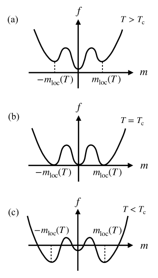
Figure 11: Free energy as a function of $m$ for $T$ fixed.

We derive $m_{\rm loc}(T)$ explicitly. We define $\sigma(T,m)$ as

$$\sigma(T,m)\equiv-\left({\frac{\partial f}{\partial m}}\right)_{T}.$$ (A.5)

The locally stable states satisfy $\sigma(T,m)=0$:

$$a_{1}(T-T_{0})m-a_{2}m^{3}+a_{3}m^{5}=0.$$ (A.6)

Non-trivial solutions other than $m=0$ satisfy

$$T=T_{0}+\frac{a_{2}}{a_{1}}m^{2}-\frac{a_{3}}{a_{1}}m^{4},$$ (A.7)

where the right-hand side is written as $T(m)$. See Fig. 12. In order to seek the solutions, we consider

$$a_{1}T^{\prime}(m)=2a_{2}m-4a_{3}m^{3}=0,$$ (A.8)

which gives $m=0$ and $m=\pm m_{1}$ with

$$m_{1}=\sqrt{\frac{a_{2}}{2a_{3}}}.$$ (A.9)

By setting

$$T_{1}=T(m_{1})=T_{0}+\frac{a_{2}^{2}}{4a_{1}a_{3}},$$ (A.10)

we find three locally stable states $m=0$ and $m=\pm m_{\rm loc}(T)$ when $T_{0}\leq T\leq T_{1}$, where $m_{\rm loc}(T)>0$ is given by

$$m_{\rm loc}(T)=\sqrt{\frac{a_{2}+\sqrt{a_{2}^{2}-4a_{1}a_{3}(T-T_{0})}}{2a_{3}}}.$$ (A.11)

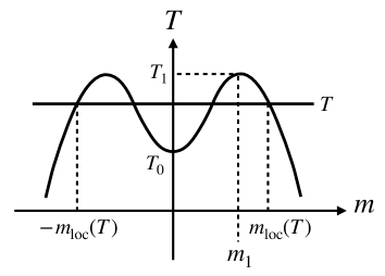
Figure 12: $T(m)$ as a function of $m$.

A.2 Entropy density

The entropy density $s(T,m)$ is given by

$$s = -\left({\frac{\partial f}{\partial T}}\right)_{m}$$ (A.12)

$$= -\frac{a_{1}}{2}m^{2}-\varphi^{\prime}(T).$$ (A.13)

The internal energy density $u(T,m)$ is determined as

$$u(T,m)=-\frac{a_{1}}{2}T_{0}m^{2}-\frac{a_{2}}{4}m^{4}+\frac{a_{3}}{6}m^{6}+\varphi(T)-T\varphi^{\prime}(T).$$ (A.14)

For simplicity, we assume that the heat capacity per unit volume, which is defined as

$$c_{m}=\left({\frac{\partial u}{\partial T}}\right)_{m},$$ (A.15)

is constant. Then, the last two terms of $u(T,m)$ should be $c_{m}T$ up to an additive constant. This leads to

$$\varphi^{\prime}(T)=-c_{m}\log T+{\rm const}.$$ (A.16)

From (A.14), we then derive

$$T(u,m)=\frac{1}{c_{m}}\left[u+\frac{a_{1}}{2}T_{0}m^{2}+\frac{a_{2}}{4}m^{4}-\frac{a_{3}}{6}m^{6}\right].$$ (A.17)

By substituting this into (A.13) with (A.16), we obtain the entropy density as a function of $(u,m)$:

$$s(u,m) =-\frac{a_{1}}{2}m^{2}$$

$$+c_{m}\log\left[u+\frac{a_{1}}{2}T_{0}m^{2}+\frac{a_{2}}{4}m^{4}-\frac{a_{3}}{6}m^{6}\right]$$ (A.18)

up to an additive constant.

By rewriting (A.12) as

$$s(u,m)=-\left.\frac{\partial f(T,m)}{\partial T}\right|_{T=T(u,m)},$$ (A.19)

we obtain

$$\left({\frac{\partial s}{\partial u}}\right)_{m}=\frac{1}{T}.$$ (A.20)

By noting $f=u-Ts$, we also rewrite (A.5) as

$$\sigma=T(u,m)\left({\frac{\partial s}{\partial m}}\right)_{u}.$$ (A.21)

These relations, (A.20) and (A.21), are summarized as (II.6).

Appendix B Precise form of the stochastic model

A formal expression of the stochastic model was immediately obtained in Sec. II.3. However, due to the multiplicative nature of the noise, the formal model exhibits a singular behavior. Therefore, we must perform a careful analysis of the stochastic process by appropriately choosing the short-length cut-off of the noise. It should be noted that the singularity is specific to the dynamics of non-conserved quantities and that it does not appear in the standard fluctuating hydrodynamics Zubarev-Morozov ; Morozov . In this section, by a theoretical argument using the separation of scales, we obtain a consistent stochastic model. We do not find references that mention this remark, but this is not surprising even if it was well-recognized by specialists in the 1970’s. In Appendix B.1, after some preliminaries, we write a normal form of the Onsager theory. In Appendix B.2, we derive the stochastic model with precisely specifying the noise property.

B.1 Preliminaries for the derivation

In order to derive the stochastic model, we rewrite the set of deterministic equations, (II.31), (II.32), and (II.33), as the simplest form. The key concept here is to introduce ${\boldsymbol{q}}$ by

$$\phi=\frac{E}{LL_{y}L_{z}}+{\boldsymbol{\nabla}}{\boldsymbol{q}},$$ (B.1)

where we impose ${\boldsymbol{q}}{\boldsymbol{n}}=0$ at the boundaries so as to satisfy (II.19). We express (B.1) as $\phi=\phi({\boldsymbol{q}})$. We here note

$${\cal S}(m,v,\phi({\boldsymbol{q}}+\delta{\boldsymbol{q}}))-{\cal S}(m,v,\phi({\boldsymbol{q}}))$$

$$=\int d^{3}{\boldsymbol{r}}\left.\frac{\delta\cal S}{\delta\phi({\boldsymbol{r}})}\right|_{\phi=\phi({\boldsymbol{q}})}{\boldsymbol{\nabla}}\delta{\boldsymbol{q}}({\boldsymbol{r}})$$

$$=\int d^{3}{\boldsymbol{r}}{\boldsymbol{\nabla}}\left[\left.\frac{\delta\cal S}{\delta\phi({\boldsymbol{r}})}\right|_{\phi=\phi({\boldsymbol{q}})}\delta{\boldsymbol{q}}({\boldsymbol{r}})\right]$$

$$\qquad\qquad-\int d^{3}{\boldsymbol{r}}{\boldsymbol{\nabla}}\left[\left.\frac{\delta\cal S}{\delta\phi({\boldsymbol{r}})}\right|_{\phi=\phi({\boldsymbol{q}})}\right]\delta{\boldsymbol{q}}({\boldsymbol{r}})$$

$$=-\int d^{3}{\boldsymbol{r}}{\boldsymbol{\nabla}}\left[\left.\frac{\delta\cal S}{\delta\phi({\boldsymbol{r}})}\right|_{\phi=\phi({\boldsymbol{q}})}\right]\delta{\boldsymbol{q}}({\boldsymbol{r}}),$$ (B.2)

where we have used the boundary condition ${\boldsymbol{q}}{\boldsymbol{n}}=0$. We simply express the result (B.2) as

$$\frac{\delta\cal S}{\delta{\boldsymbol{q}}({\boldsymbol{r}})}=-{\boldsymbol{\nabla}}\frac{\delta\cal S}{\delta\phi({\boldsymbol{r}})}.$$ (B.3)

By using this expression and substituting (B.1) into (II.33), we rewrite (II.33) as

$$\partial_{t}{\boldsymbol{q}}=\lambda\frac{\delta\cal S}{\delta{\boldsymbol{q}}({\boldsymbol{r}})}+{\boldsymbol{B}},$$ (B.4)

where ${\boldsymbol{B}}$ satisfies

$${\boldsymbol{\nabla}}{\boldsymbol{B}}=0.$$ (B.5)

For a given $\phi$, ${\boldsymbol{\nabla}}\times{\boldsymbol{q}}$ may take arbitrary values. We fix this value at time $t$ by the solution of the equation

$$\partial_{t}({\boldsymbol{\nabla}}\times{\boldsymbol{q}})={\boldsymbol{\nabla}}\times\lambda\frac{\delta\cal S}{\delta{\boldsymbol{q}}({\boldsymbol{r}})}$$ (B.6)

with the initial value ${\boldsymbol{\nabla}}\times{\boldsymbol{q}}={\boldsymbol{0}}$ at $t=0$. Under this fixing condition, we have ${\boldsymbol{\nabla}}\times{\boldsymbol{B}}={\boldsymbol{0}}$. Together with (B.5), we find that ${\boldsymbol{B}}$ is constant in ${\boldsymbol{r}}$. Finally, noting the condition that ${\boldsymbol{q}}{\boldsymbol{n}}=0$ and ${\boldsymbol{\nabla}}\beta{\boldsymbol{n}}=0$ at the boundary, we have ${\boldsymbol{B}}{\boldsymbol{n}}=0$ from (B.4). We thus derive

$${\boldsymbol{B}}={\boldsymbol{0}}.$$ (B.7)

Substituting this result into (B.4), we obtain

$$\partial_{t}{\boldsymbol{q}}=\lambda\frac{\delta\cal S}{\delta{\boldsymbol{q}}({\boldsymbol{r}})}.$$ (B.8)

As shown below, the variable ${\boldsymbol{q}}$ is convenient to analyze the stochastic model. As far as we checked, there are no references that introduce the variable ${\boldsymbol{q}}$ instead of a locally conserved quantity.

Here, we define the five components field

$$\chi\equiv(m,v,q_{x},q_{y},q_{z}),$$ (B.9)

and $\chi^{a}$ $(a=1,2,\cdots,5)$ denotes each component. For any functional of $\alpha=(m,v,\phi)$, such as ${\cal S}(\alpha)$ and ${\cal P}_{\rm eq}(\alpha)$, we define the functional of $\chi$ through $\alpha=\alpha(\chi)$. For example, ${\cal P}_{\rm eq}(\chi)$ represents ${\cal P}_{\rm eq}(\alpha(\chi))$. The set of equations (II.31), (II.32), and (B.8) is expressed as

$$\partial_{t}\chi^{a}=\sum_{b=1}^{5}L^{ab}(\chi({\boldsymbol{r}}),\nabla\chi({\boldsymbol{r}}))\frac{\delta\cal S}{\delta\chi^{b}({\boldsymbol{r}})},$$ (B.10)

where $L^{12}=-L^{21}=-T$, $L^{22}=\gamma T$, $L^{33}=L^{44}=L^{55}=\lambda$, and $L^{ab}=0$ for the other components. It should be noted that $T$ and $\lambda$ are functions of $(u,m)$, while $\gamma$ is a constant. Since

$$u=\frac{E}{LL_{y}L_{z}}+{\boldsymbol{\nabla}}{\boldsymbol{q}}-\frac{v^{2}}{2}-d_{e}\frac{|{\boldsymbol{\nabla}}m|^{2}}{2},$$ (B.11)

$L^{ab}(\chi({\boldsymbol{r}}),\nabla\chi({\boldsymbol{r}}))$ is determined from $\chi$ and $\nabla\chi$ for each ${\boldsymbol{r}}$.

Now, the stochastic model is constructed so as to satisfy the detailed balance condition with respect to the stationary distribution ${\cal P}_{\rm eq}(\chi)$. If we ignore $v$ dependence of $T$ with fixed $(m,{\boldsymbol{q}})$, the model would be immediately obtained as

$$\partial_{t}\chi^{a}=\sum_{b=1}^{5}L^{ab}(\chi({\boldsymbol{r}}),\nabla\chi({\boldsymbol{r}}))\frac{\delta\cal S}{\delta\chi^{b}({\boldsymbol{r}})}+\sqrt{2L^{aa}}\xi^{a}.$$ (B.12)

See e.g. Graham . The model is identical to the formal model introduced in Sec. II.3. Unfortunately, however, we cannot ignore $v$ dependence of $T$ so as to satisfy the detailed balance condition. To make the matter worse, the contribution gives a spurious divergence, as will be seen in the next subsection.

In order to resolve this problem, we notice that the noises should have a finite correlation length because the noises appear as the result of coarse-graining of microscopic mechanical degrees of freedom Zwanzig . We describe this property by introducing a cutoff $\Lambda_{c}$ for the noise and replace (II.53) by

$$\left\langle\xi^{a}({\boldsymbol{r}},t)\xi^{b}({\boldsymbol{r}}^{\prime},t^{\prime})\right\rangle = \delta^{ab}\delta_{\Lambda_{c}}({\boldsymbol{r}}-{\boldsymbol{r}^{\prime}})\delta(t-t^{\prime})$$ (B.13)

with

$$\delta_{\Lambda_{c}}({\boldsymbol{r}})=\int_{|{\boldsymbol{k}}|\Lambda_{c}<1}\frac{d^{3}{\boldsymbol{k}}}{(2\pi)^{3}}e^{i{\boldsymbol{k}}{\boldsymbol{r}}}.$$ (B.14)

Here, the cut-off length $\Lambda_{c}$ is much larger than the microscopic length scale $\ell$ and much shorter than the coarse-grained size $\Lambda$. We thus impose

$$\ell\ll\Lambda_{c}\ll\Lambda\ll L.$$ (B.15)

The condition $\ell\ll\Lambda_{c}$ is necessary to remove a singular term associated with the multiplicative nature of the noise, which will be discussed below. This cut-off induces the non-local coupling between the Onsager coefficients and the thermodynamic forces. Since the length of the non-local coupling is $\Lambda_{c}$ and the spatial variation of the variables is larger than $\Lambda$, we can approximate it by the local coupling ignoring the contribution of $O(\Lambda_{c}/\Lambda)$. We will give a precise argument for the derivation of the model in Appendix B.2.

Summarizing these results, we write the stochastic model as

$$\partial_{t}m=T\otimes{\beta v},$$ (B.16)

$$\partial_{t}v=-\gamma T\otimes\beta v+T\otimes\left({\frac{\partial s}{\partial m}}\right)_{u}+d_{e}T\otimes({\boldsymbol{\nabla}}\beta)({\boldsymbol{\nabla}}m)$$

$$\qquad\qquad+T\otimes d_{f}\beta\Delta m+\sqrt{2\gamma T}\otimes\xi^{v},$$ (B.17)

$$\partial_{t}\phi=-{\boldsymbol{\nabla}}\left(\lambda\otimes{\boldsymbol{\nabla}}\beta+\sqrt{2\lambda}\otimes{\boldsymbol{\xi}}^{\phi}\right),$$ (B.18)

where $f\otimes g$ is defined as

$$f\otimes g=\int\!d^{3}{\boldsymbol{r}}^{\prime}\!\!\int\!d^{3}{\boldsymbol{r}}^{\prime\prime}f({\boldsymbol{r}^{\prime\prime}})\delta_{\Lambda_{c}}({\boldsymbol{r}}-{\boldsymbol{r}}^{\prime\prime})\delta_{\Lambda_{c}}({\boldsymbol{r}}^{\prime}-{\boldsymbol{r}}^{\prime\prime})g({\boldsymbol{r}}^{\prime}).$$ (B.19)

Since $\Lambda_{c}\ll\Lambda$, (B.16), (B.17), (B.18) may be interpreted as a physical model of the the formal model (II.47), (II.48), and (II.49). It should be noted that the unsatisfactory properties of the formal model are not observed in the physical model (B.16), (B.17), and (B.18) with (B.13). Therefore, we should study the physical model. Although the expression of the physical model is rather complicated, the theoretical analysis can be done similarly to that of the formal model. Keeping this in mind, we study the formal model in the main text.

B.2 Derivation

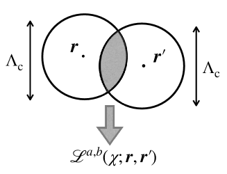
Figure 13: Schematic figure of non-local Onsager coefficient ${\cal L}^{ab}$.

Since we assume the cut-off length in the noise, (B.12) becomes a non-local form with using a functional of $\chi$ as

$${\cal L}^{ab}(\chi;{\boldsymbol{r}},{\boldsymbol{r}}^{\prime}) \equiv \int d^{3}{\boldsymbol{r}}^{\prime\prime}L^{ab}(\chi({\boldsymbol{r}}^{\prime\prime}),\nabla\chi({\boldsymbol{r}}^{\prime\prime}))$$ (B.20)

$$\times\delta_{\Lambda_{c}}({\boldsymbol{r}}-{\boldsymbol{r}}^{\prime\prime})\delta_{\Lambda_{c}}({\boldsymbol{r}}^{\prime}-{\boldsymbol{r}}^{\prime\prime}),$$

which is illustrated in Fig. 13. Further, since the Onsager coefficients $L^{ab}$ in (B.10) depend on $\chi$, we have to consider multiplicative nature of the noise in the stochastic dynamics. From these, the stochastic model (B.12) is replaced by

$$\partial_{t}\chi^{a} = \sum_{b}\int d^{3}{\boldsymbol{r}}^{\prime}\left[{\cal L}^{ab}(\chi;{\boldsymbol{r}},{\boldsymbol{r}}^{\prime})\frac{\delta\cal S}{\delta\chi^{b}({\boldsymbol{r}}^{\prime})}\right.$$ (B.21)

$$\left.+\frac{\delta{\cal L}^{ab}(\chi;{\boldsymbol{r}},{\boldsymbol{r}}^{\prime})}{\delta\chi^{b}({\boldsymbol{r}}^{\prime})}\delta^{ab}\right]$$

$$+\int d^{3}{\boldsymbol{r}}^{\prime}{\cal G}^{a}(\chi;{\boldsymbol{r}},{\boldsymbol{r}}^{\prime})\cdot\xi^{a}({\boldsymbol{r}}^{\prime}),$$

where the functional ${\cal G}^{a}(\chi;{\boldsymbol{r}},{\boldsymbol{r}}^{\prime})$ is determined later and the symbol ‘$\cdot$’ in front of $\xi^{a}$ represents the Ito multiplication. The second term on the right-hand side of (B.21) is necessary to yield the equilibrium stationary distribution (II.46) Graham ; Itami-Sasa . Here, it should be noted that the off-diagonal components of ${\cal L}^{ab}$ do not appear in the second term, because the terms with off-diagonal components of ${\cal L}^{ab}$ do not contribute to the entropy production. See Itami-Sasa for the detail.

The Fokker-Planck equation for the probability density ${\cal P}(\chi,t)$ corresponding to (B.21) is written as

$$\partial_{t}{\cal P}(\chi,t)+\sum_{ab}\int d^{3}{\boldsymbol{r}}d^{3}{\boldsymbol{r}}^{\prime}\frac{\delta}{\delta\chi^{a}({\boldsymbol{r}})}\left[{\cal A}^{ab}(\chi;{\boldsymbol{r}},{\boldsymbol{r}}^{\prime}){\cal P}(\chi,t)\right]$$

$$=\frac{1}{2}\sum_{a}\int d^{3}{\boldsymbol{r}}d^{3}{\boldsymbol{r}}^{\prime}\frac{\delta^{2}}{\delta\chi^{a}({\boldsymbol{r}})\delta\chi^{a}({\boldsymbol{r}}^{\prime})}[{\cal B}^{a}(\chi;{\boldsymbol{r}},{\boldsymbol{r}}^{\prime}){\cal P}(\chi,t)]$$ (B.22)

with

$${\cal A}^{ab}(\chi;{\boldsymbol{r}},{\boldsymbol{r}}^{\prime})\equiv{\cal L}^{ab}(\chi;{\boldsymbol{r}},{\boldsymbol{r}}^{\prime})\frac{\delta\cal S}{\delta\chi^{b}({\boldsymbol{r}}^{\prime})}+\delta^{ab}\frac{\delta{\cal L}^{ab}(\chi;{\boldsymbol{r}},{\boldsymbol{r}}^{\prime})}{\delta\chi^{b}({\boldsymbol{r}}^{\prime})},$$ (B.23)

$${\cal B}^{a}(\chi;{\boldsymbol{r}},{\boldsymbol{r}}^{\prime})$$

$$\equiv\int d^{3}{\boldsymbol{r}^{\prime\prime}}d^{3}{\boldsymbol{r}}^{\prime\prime\prime}{\cal G}^{a}(\chi;{\boldsymbol{r}},{\boldsymbol{r}}^{\prime\prime}){\cal G}^{a}(\chi;{\boldsymbol{r}}^{\prime},{\boldsymbol{r}}^{\prime\prime\prime})\delta_{\Lambda_{c}}({\boldsymbol{r}}^{\prime\prime}-{\boldsymbol{r}}^{\prime\prime\prime}).$$ (B.24)

Here, as shown in Itami-Sasa ; Graham , the detailed balance condition is expressed as

$$\int d^{3}{\boldsymbol{r}}\frac{\delta}{\delta\chi^{1}({\boldsymbol{r}})}\left[{\cal L}^{12}(\chi;{\boldsymbol{r}},{\boldsymbol{r}}^{\prime})\frac{\delta\cal S}{\delta\chi^{2}({\boldsymbol{r}}^{\prime})}{\cal P}_{\rm eq}(\chi)\right]$$

$$+\int d^{3}{\boldsymbol{r}}\frac{\delta}{\delta\chi^{2}({\boldsymbol{r}})}\left[{\cal L}^{21}(\chi;{\boldsymbol{r}},{\boldsymbol{r}}^{\prime})\frac{\delta\cal S}{\delta\chi^{1}({\boldsymbol{r}}^{\prime})}{\cal P}_{\rm eq}(\chi)\right]=0,$$ (B.25)

$$2{\cal L}^{aa}(\chi;{\boldsymbol{r}},{\boldsymbol{r}}^{\prime})={\cal B}^{a}(\chi;{\boldsymbol{r}},{\boldsymbol{r}}^{\prime}),$$ (B.26)

which leads to the stationary distribution (II.46). We thus have to confirm (B.25) and (B.26).

First, we estimate the left-hand side of (B.25). From the anti-symmetric property

$${\cal L}^{12}(\chi;{\boldsymbol{r}},{\boldsymbol{r}}^{\prime})=-{\cal L}^{21}(\chi;{\boldsymbol{r}}^{\prime},{\boldsymbol{r}}),$$ (B.27)

the left-hand side of (B.25) is written as

$$\int d^{3}{\boldsymbol{r}}\frac{\delta{\cal L}^{12}(\chi;{\boldsymbol{r}},{\boldsymbol{r}}^{\prime})}{\delta\chi^{1}({\boldsymbol{r}})}\frac{\delta\cal S}{\delta\chi^{2}({\boldsymbol{r}}^{\prime})}{\cal P}_{\rm eq}(\chi)$$

$$\quad+\int d^{3}{\boldsymbol{r}}\frac{\delta{\cal L}^{21}(\chi;{\boldsymbol{r}},{\boldsymbol{r}}^{\prime})}{\delta\chi^{2}({\boldsymbol{r}})}\frac{\delta\cal S}{\delta\chi^{1}({\boldsymbol{r}}^{\prime})}{\cal P}_{\rm eq}(\chi).$$ (B.28)

We here explicitly calculate

$$\int d^{3}{\boldsymbol{r}}\frac{\delta{\cal L}^{12}(\chi;{\boldsymbol{r}},{\boldsymbol{r}}^{\prime})}{\delta\chi^{1}({\boldsymbol{r}})} = -\left({\frac{\partial T}{\partial m}}\right)_{u}\delta_{\Lambda_{c}}(0)$$ (B.29)

$$= \frac{1}{c_{m}}\left({\frac{\partial u}{\partial m}}\right)_{T}\delta_{\Lambda_{c}}(0),$$

where we have used $\delta_{\Lambda_{c}}^{\prime}(0)=0$. Similarly, we have

$$\int d^{3}{\boldsymbol{r}}\frac{\delta{\cal L}^{21}(\chi;{\boldsymbol{r}},{\boldsymbol{r}}^{\prime})}{\delta\chi^{2}({\boldsymbol{r}})} = \left({\frac{\partial T}{\partial u}}\right)_{m}\left({\frac{\partial u}{\partial v}}\right)_{{\boldsymbol{q}},m}\delta_{\Lambda_{c}}(0)$$ (B.30)

$$= -\frac{v}{c_{m}}\delta_{\Lambda_{c}}(0).$$

These expressions involve the dimensionless quantity $\delta_{\Lambda_{c}}(0)/c_{m}$. Since $\delta_{\Lambda_{c}}(0)=O(\Lambda_{c}^{-3})$ and $c_{m}=O(\ell^{-3})$, $\delta_{\Lambda_{c}}(0)/c_{m}$ is estimated as $O(\ell^{3}/\Lambda_{c}^{3})$. This leads to

$$\int d^{3}{\boldsymbol{r}}\frac{\delta{\cal L}^{12}(\chi;{\boldsymbol{r}},{\boldsymbol{r}}^{\prime})}{\delta\chi^{1}({\boldsymbol{r}})} = \left({\frac{\partial u}{\partial m}}\right)_{T}O\left(\frac{\ell^{3}}{\Lambda_{c}^{3}}\right),$$ (B.31)

$$\int d^{3}{\boldsymbol{r}}\frac{\delta{\cal L}^{21}(\chi;{\boldsymbol{r}},{\boldsymbol{r}}^{\prime})}{\delta\chi^{2}({\boldsymbol{r}})} = {v}\left(\frac{\ell^{3}}{\Lambda_{c}^{3}}\right)$$ (B.32)

in the asymptotic limit $\ell/\Lambda_{c}\to 0$. By substituting (B.31) and (B.32) into (B.28), we find that (B.28) is proportional to $O(\ell^{3}/\Lambda_{c}^{3})$, which is zero in the limit (B.15). Then, we have confirmed (B.25). Note that (B.31) and (B.32) exhibit the divergence without the cutoff $\Lambda_{c}$. This apparent divergence becomes zero in the appropriate limit after introducing the cut-off $\Lambda_{c}$. Such an asymptotic estimate using a similar cut-off was used in Ref. Nakano .

Next, we determine ${\cal G}^{a}$ from the condition (B.26). We note that (B.26) is satisfied when

$$2L^{aa}(\chi({\boldsymbol{r}}^{\prime\prime}),\nabla\chi({\boldsymbol{r}}^{\prime\prime}))\delta_{\Lambda_{c}}({\boldsymbol{r}}-{\boldsymbol{r}}^{\prime\prime})\delta_{\Lambda_{c}}({\boldsymbol{r}}^{\prime}-{\boldsymbol{r}}^{\prime\prime})$$

$$=\int d^{3}{\boldsymbol{r}}^{\prime\prime\prime}{\cal G}^{a}(\chi;{\boldsymbol{r}},{\boldsymbol{r}}^{\prime\prime}){\cal G}^{a}(\chi;{\boldsymbol{r}}^{\prime},{\boldsymbol{r}}^{\prime\prime\prime})\delta_{\Lambda_{c}}({\boldsymbol{r}^{\prime\prime}}-{\boldsymbol{r}^{\prime\prime\prime}}).$$ (B.33)

By substituting

$${\cal G}^{a}(\chi;{\boldsymbol{r}},{\boldsymbol{r}}^{\prime})=\int d^{3}{\boldsymbol{r}}^{\prime\prime}\sqrt{2L^{aa}(\chi({\boldsymbol{r}}^{\prime\prime}),\nabla\chi({\boldsymbol{r}}^{\prime\prime}))}$$

$$\qquad\times\delta_{\Lambda_{c}}({\boldsymbol{r}}-{\boldsymbol{r}}^{\prime\prime})\delta_{\Lambda_{c}}({\boldsymbol{r}}^{\prime}-{\boldsymbol{r}}^{\prime\prime})$$

$$\qquad\times\left[1+O\left(\frac{\Lambda_{c}^{3}}{\Lambda^{3}}\right)\right]$$ (B.34)

into the right-hand side of (B.33), we confirm that the right-hand side is equal to the left-hand side of (B.33) with an error of $O((\Lambda_{c}/\Lambda)^{3})$. Therefore, we claim that the condition (B.26) holds.

Finally, we investigate the second term in the right-hand side of (B.21). We concretely calculate each term as follows.

$$\int d^{3}{\boldsymbol{r}}^{\prime}\frac{\delta{\cal L}^{22}(\chi;{\boldsymbol{r}},{\boldsymbol{r}}^{\prime})}{\delta\chi^{2}({\boldsymbol{r}}^{\prime})} = \gamma\left({\frac{\partial T}{\partial u}}\right)_{m}\left({\frac{\partial u}{\partial v}}\right)_{{\boldsymbol{q}},m}\delta_{\Lambda_{c}}(0)$$ (B.35)

$$= -\gamma vO\left(\frac{\ell^{3}}{\Lambda_{c}^{3}}\right),$$

and

$$\int d^{3}{\boldsymbol{r}}^{\prime}\frac{\delta{\cal L}^{33}(\chi;{\boldsymbol{r}},{\boldsymbol{r}}^{\prime})}{\delta\chi^{3}({\boldsymbol{r}}^{\prime})} = 0,$$ (B.36)

where we have used $\delta_{\Lambda_{c}}^{\prime}(0)=0$. (B.35) provides a correction of the momentum dissipation term $-\gamma v$. This correction can be negligible from the condition (B.15). Therefore, the second term in the right-hand side of (B.21) can be ignored. We here remark that the equality (B.36) leads to the statement that the multiplication rule of the noise, Ito or Stratonovich, is irrelevant for the standard fluctuating hydrodynamics Zubarev-Morozov ; Morozov .

More explicitly, by considering a physical situation, we may estimate $\eta=10^{-8}$. Recalling $\Lambda/L=O(\sqrt{\eta})$, we express (B.15) by

$$\sqrt{\eta}\ll\frac{\Lambda_{c}}{\Lambda}\ll 1.$$ (B.37)

As one example, we choose $\Lambda_{c}/\Lambda=10^{-2}$, which makes the theory consistent. It should be noted that we consider the case that the interface width also vanishes in the limit $\eta\to 0$, which is in contrast to the standard weak noise limit Bertini-rev . This aspect brings non-trivial noise effects even in the limit $\eta\to 0$.

Appendix C Derivation of (IV.5)

In this Appendix, we derive (IV.5). In order to simplify the notation, we omit $E$ dependence such that ${\cal P}(\alpha,t_{f};E,J)$ is expressed as ${\cal P}(\alpha,t_{f};J)$. Following the notation in the main text, we define $\alpha^{\dagger}$ for $\alpha=(m,v,\phi)$ as $\alpha^{\dagger}=(m,-v,\phi)$ and $\hat{\alpha}^{\dagger}$ denotes the time-reversal of $\hat{\alpha}$. That is,

$$\hat{\alpha}^{\dagger}(t)=(m(t_{f}-t),-v(t_{f}-t),\phi(t_{f}-t)).$$

We first substitute the dimensionless version of (II.27) and (II.28),

$$\frac{\delta\cal S}{\delta m({\boldsymbol{r}})}=\beta\sigma+\eta[d_{e}({\boldsymbol{\nabla}}\beta)({\boldsymbol{\nabla}}m)+\beta d_{f}\Delta m],$$ (C.1)

$$\frac{\delta\cal S}{\delta v({\boldsymbol{r}})}=-{\beta v},$$ (C.2)

into (IV.2) and a similar expression of $\hat{\cal I}(\hat{\alpha}^{\dagger}|(\alpha(t_{f}))^{\dagger};-J)$. By noting

$${\boldsymbol{j}}{\boldsymbol{\nabla}}\beta = {\boldsymbol{\nabla}}({\boldsymbol{j}}\beta)-\beta{\boldsymbol{\nabla}}{\boldsymbol{j}}$$ (C.3)

$$= {\boldsymbol{\nabla}}({\boldsymbol{j}}\beta)+\frac{\delta\cal S}{\delta\phi({\boldsymbol{r}})}\partial_{t}\phi,$$

we obtain

$$\hat{\cal I}(\hat{\alpha}|\alpha(0);J)-\hat{\cal I}(\hat{\alpha}^{\dagger}|(\alpha(t_{f}))^{\dagger};-J)$$

$$=-\int_{0}^{t_{f}}dt\int d^{3}{\boldsymbol{r}}\left[(\partial_{t}m)\frac{\delta\cal S}{\delta m({\boldsymbol{r}})}+(\partial_{t}v)\frac{\delta\cal S}{\delta v({\boldsymbol{r}})}\right.$$

$$\hskip 28.45274pt+\left.{\boldsymbol{\nabla}}\left({\boldsymbol{j}}\beta\right)+(\partial_{t}\phi)\frac{\delta\cal S}{\delta\phi({\boldsymbol{r}})}\right],$$ (C.4)

which leads to

$$\hat{\cal I}(\hat{\alpha}|\alpha(0);J)-\hat{\cal I}(\hat{\alpha}^{\dagger}|(\alpha(t_{f}))^{\dagger};-J)$$

$$=-{\cal S}(\alpha(t_{f}))+{\cal S}(\alpha(0))$$

$$-J\int d^{2}{\boldsymbol{r}}_{\perp}\int_{0}^{t_{f}}dt(\beta(1,{\boldsymbol{r}}_{\perp},t)-\beta(0,{\boldsymbol{r}}_{\perp},t)),$$ (C.5)

where ${\boldsymbol{r}}_{\perp}=(y,z)$.

Now, for an initial distribution ${\cal P}_{0}$, the distribution at $t=t_{f}$ is expressed as

$${\cal P}(\alpha,t_{f};J)=\int{\cal D}\hat{\alpha}{\cal P}_{0}(\alpha(0))\hat{\cal P}(\hat{\alpha}|\alpha(0);J)\delta(\alpha(t_{f})-\alpha).$$ (C.6)

Here, as a special choice, we take

$${\cal P}_{0}(\alpha)={\cal N}\exp\left(\frac{1}{\eta^{3}}{\cal S}(\alpha)\right)\delta\left(\int d^{3}{\boldsymbol{r}}\phi({\boldsymbol{r}})-E\right).$$ (C.7)

From (C.5), we find

$$\frac{\hat{\cal P}(\hat{\alpha}|\alpha(0);J){\cal P}_{0}(\alpha(0))}{\hat{\cal P}(\hat{\alpha}^{\dagger}|(\alpha(t_{f}))^{\dagger};-J){\cal P}_{0}((\alpha(t_{f}))^{\dagger})}$$

$$=\exp\left(\frac{J}{\eta^{3}}\int d^{2}{\boldsymbol{r}}_{\perp}\int_{0}^{t_{f}}dt(\beta(1,{\boldsymbol{r}}_{\perp},t)-\beta(0,{\boldsymbol{r}}_{\perp},t))\right).$$ (C.8)

We then rewrite (C.6) as

$${\cal P}(\alpha,t_{f};J)=\int{\cal D}\hat{\alpha}{\cal P}_{0}((\alpha(t_{f}))^{\dagger})\hat{\cal P}(\hat{\alpha}^{\dagger}|(\alpha(t_{f})^{\dagger};-J)$$

$$\times\frac{{\cal P}_{0}(\alpha(0))\hat{\cal P}(\hat{\alpha}|\alpha(0);J)}{{\cal P}_{0}((\alpha(t_{f}))^{\dagger})\hat{\cal P}(\hat{\alpha}^{\dagger}|(\alpha(t_{f}))^{\dagger};-J)}\delta(\alpha(t_{f})-\alpha).$$ (C.9)

The substitution of (C.8) into the right-hand side yields

$$\int{\cal D}\hat{\alpha}^{\dagger}{\cal P}_{0}((\alpha(t_{f}))^{\dagger})\hat{\cal P}(\hat{\alpha}^{\dagger}|(\alpha(t_{f}))^{\dagger};-J)$$

$$\quad\times{\rm e}^{J/\eta^{3}\int d^{2}{\boldsymbol{r}}_{\perp}\int_{0}^{t_{f}}dt(\beta(1,{\boldsymbol{r}}_{\perp},t)-\beta(0,{\boldsymbol{r}}_{\perp},t))}$$

$$\qquad\times\delta((\alpha(t_{f}))^{\dagger}-\alpha^{\dagger}).$$ (C.10)

By using the transformation $\hat{\alpha}\to\hat{\alpha}^{\dagger}$ in the path integral variable, (C.10) is written as

$$\int{\cal D}\hat{\alpha}{\cal P}_{0}(\alpha(0))\hat{\cal P}(\hat{\alpha}|\alpha(0);-J)$$

$$\quad\times{\rm e}^{J/\eta^{3}\int d{\boldsymbol{r}}_{\perp}\int_{0}^{t_{f}}dt(\beta(1,{\boldsymbol{r}}_{\perp},t)-\beta(0,{\boldsymbol{r}}_{\perp},t))}$$

$$\qquad\times\delta(\alpha(0)-\alpha^{\dagger}),$$ (C.11)

where we have used

$$\int_{0}^{t_{f}}dt\beta(1,{\boldsymbol{r}_{\perp}},t_{f}-t) =-\int_{t_{f}}^{0}dt^{\prime}\beta(1,{\boldsymbol{r}_{\perp}},t^{\prime})$$

$$=\int_{0}^{t_{f}}dt^{\prime}\beta(1,{\boldsymbol{r}_{\perp}},t^{\prime}).$$ (C.12)

By substituting (C.7) into (C.11), we finally obtain

$${\cal P}(\alpha,t_{f};J)={\cal N}{\rm e}^{{\cal S}(\alpha)/\eta^{3}}$$

$$\times\left\langle{\rm e}^{J/\eta^{3}\int d^{2}{\boldsymbol{r}}_{\perp}\int_{0}^{t_{f}}dt(\beta(1,{\boldsymbol{r}}_{\perp},t)-\beta(0,{\boldsymbol{r}}_{\perp},t))}\right\rangle_{\alpha^{\dagger}\to*}^{-J}$$

$$\times\delta\left(\int d^{3}{\boldsymbol{r}}\phi({\boldsymbol{r}})-E\right),$$ (C.13)

where $\left\langle\ \right\rangle_{\alpha\to*}^{-J}$ represents the expectation value over trajectories $\alpha(t)$ starting from $\alpha(0)=\alpha$ with respect to the path probability density in the system with $-J$.

We here remark that (C.8) is referred to as the local detailed balance condition which connects the ratio of path probabilities of forward and backward trajectories with the entropy production along the trajectory. This is the key relation for deriving many universal relations.

Appendix D Estimation of $\tau_{\rm int}$

In this Appendix, we estimate the typical time scale of the interface motion by analyzing the deterministic model (II.37), (II.38), and (II.39) with the condition that the heat conduction is sufficiently fast. Note that the model is not the dimensionless version in order to clarify the physical argument for the estimation.

We assume an initial state with an interface position $X_{0}$ and a uniform temperature $T^{\rm qeq}_{X_{0}}\not=T_{c}$, which satisfies

$$X_{0}u^{\rm o}(T^{\rm qeq}_{X_{0}})+(L-X_{0})u^{\rm d}(T^{\rm qeq}_{X_{0}})=\frac{E}{L_{y}L_{z}},$$ (D.1)

and

$$m(x,0) = m^{\rm qeq}(x-X_{0};X_{0}),$$ (D.2)

$$v(x,0) = 0$$ (D.3)

with

$$m^{\rm qeq}(x-X;X)\equiv\bar{\bar{m}}\left(\frac{x-X}{\sqrt{\eta}}\right)m_{\rm loc}(T^{\rm qeq}_{X}).$$ (D.4)

When $0<\eta\ll 1$, the interface slowly moves to the equilibrium position $X_{\rm eq}$, as shown in Fig. 14. The initial state corresponds to the quasi-equilibrium state in thermodynamics, because $T^{\rm qeq}_{X_{0}}\not=T_{c}$. The time evolution describes the transition from the quasi-equilibrium state $T^{\rm qeq}_{X_{0}}$ to the true equilibrium state $T_{c}$. We describe this interface motion quantitatively.

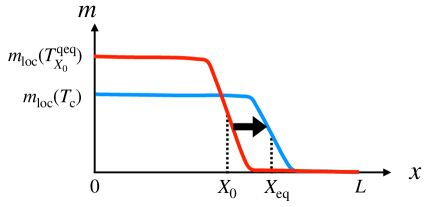
Figure 14: Schematic figure of interface motion from the quasi-equilibrium state to the equilibrium state.

Let $X(t)$ be the position of the interface at time $t$. We assume that the interface motion is slowest which will be confirmed by (D.25) in a self-consistent manner. Then, the other dynamical variables are slaved to the slow variable $X(t)$. Based on this picture, we set

$$m(x,t)=m^{\rm qeq}(x-X(t);X(t))+m^{\prime}(x,t),$$ (D.5)

$$T(x,t)=T^{\rm qeq}_{X(t)}+T^{\prime}(x,t),$$ (D.6)

$$v(x,t)=\partial_{t}m(x,t),$$ (D.7)

where $m^{\prime}$ and $T^{\prime}$ are small corrections, which are neglected in the lowest order calculation.

The temperature $T^{\rm qeq}_{X(t)}$ satisfies

$$X(t)u^{\rm o}(T^{\rm qeq}_{X(t)})+(L-X(t))u^{\rm d}(T^{\rm qeq}_{X(t)})=\frac{E}{L_{y}L_{z}}$$ (D.8)

for the interface position $X(t)$. We now attempt to determine $m^{\rm qeq}(x-X(t);X(t))$ for small $\eta$. Here, since $m^{\rm qeq}(x-X(t);X(t))$ is slowly evolving,

$$\partial_{t}^{2}m^{\rm qeq}\ll\gamma\partial_{t}m^{\rm qeq},$$ (D.9)

which will be checked by (D.25). By substituting (D.5), (D.6), and (D.7) into (II.38), we obtain

$$-\gamma\frac{dX}{dt}\partial_{x}m^{\rm qeq}=-\left.\frac{\partial f(T^{\rm qeq}_{X(t)},m)}{\partial m}\right|_{m=m^{\rm qeq}}+d_{f}\partial_{x}^{2}m^{\rm qeq},$$ (D.10)

where we have used (D.9). More precisely, although the left-hand side should be

$$-\gamma\frac{dX}{dt}\left[\partial_{x}m^{\rm qeq}-m^{\rm qeq}\frac{\partial}{\partial X}\log m_{\rm loc}(T_{X}^{\rm qeq})\right],$$ (D.11)

the second term can be ignored for small $\eta$, because the first term in the square bracket is $O(m_{\rm loc}/\Lambda)$ and the second term is $O(m_{\rm loc}/L)$. In the limit $\eta\to 0$, we consider (D.10) as the differential equation defined in $x-X(t)\in[-\infty,\infty]$ with the boundary condition

$$m^{\rm qeq}(x-X(t);X(t))\to m_{\rm loc}(T^{\rm qeq}_{X(t)})$$ (D.12)

for $x-X(t)\to-\infty$, and

$$m^{\rm qeq}(x-X(t);X(t))\to 0$$ (D.13)

for $x-X(t)\to+\infty$. We here note that a solution of the differential equation (D.10), $m^{\rm qeq}(x-X(t);X(t))$, exists only for a special value of $dX/dt$. In other words, by solving the non-linear eigenvalue equation (D.10) with $T^{\rm qeq}_{X(t)}$ given by (D.8), we determine the eigenvalue $dX/dt$ and the solution $m^{\rm qeq}(x-X(t);X(t))$, simultaneously.

The solution of the equation (D.10) is understood by identifying (D.10) with a Newton equation for the coordinate $m^{\rm qeq}$ with a fictitious time $x^{\prime}=x-X(t)$, where the fictitious mass is $d_{f}$, the fictitious friction $\gamma dX/dt$, and the potential $-f(T^{\rm qeq}_{X(t)},m^{\rm qeq})$. The precise form of $m^{\rm qeq}(x-X(t);X(t))$ and the eigenvalue $dX/dt$ can be numerically determined by solving (D.10). Here, assuming the form $m^{\rm qeq}(x-X(t);X(t))$, we express $dX/dt$ in terms of $m^{\rm qeq}(x-X(t);X(t))$. Indeed, multiplying $\partial_{x}m^{\rm qeq}(x-X(t);X(t))$ to both sides of (D.10) and integrating them over the whole region, we obtain

$$-\gamma\frac{dX}{dt}\int_{-\infty}^{\infty}dx(\partial_{x}m^{\rm qeq})^{2}$$

$$\qquad=f(T^{\rm qeq}_{X(t)},m_{\rm loc}(T^{\rm qeq}_{X(t)}))-f(T^{\rm qeq}_{X(t)},0).$$ (D.14)

This is a rather standard analysis. See for example Ref. Pomeau . The equation (D.14) represents the equation of motion for $X$. It means that the interface moves so as to decrease the total free energy. The driving force is the free energy difference given in the right-hand side, and the left-hand side describes the friction force for the interface motion. Now, when $X(t)$ is close to $X_{\rm eq}$, we have a linear equation

$$\tau_{\rm int}\frac{dX}{dt}=-(X-X_{\rm eq}).$$ (D.15)

Then, $\tau_{\rm int}$ provides the time scale of the interface motion. Below, by analyzing (D.14), we derive $\tau_{\rm int}$.

We specifically study the case that $(X(t)-X_{\rm eq})/L$ is small. In this case, $(T^{\rm qeq}_{X}-T_{c})/T_{c}$ is also small. By recalling (A.4), we notice

$$f(T^{\rm qeq}_{X(t)},m_{\rm loc}(T^{\rm qeq}_{X(t)}))-f(T^{\rm qeq}_{X(t)},0)$$

$$~{}~{}=f(T^{\rm qeq}_{X(t)},m_{\rm loc}(T^{\rm qeq}_{X(t)}))-f(T_{c},m_{\rm loc}(T_{c}))$$

$$\qquad-[f(T^{\rm qeq}_{X(t)},0)-f(T_{c},0)].$$ (D.16)

We thus estimate

$$f(T^{\rm qeq}_{X(t)},m_{\rm loc}(T^{\rm qeq}_{X(t)}))-f(T^{\rm qeq}_{X(t)},0)$$

$$=-[s(T_{c},m_{\rm loc}(T_{c}))-s(T_{c},0)](T^{\rm qeq}_{X(t)}-T_{c})$$

$$=-\frac{u^{\rm o}(T_{c})-u^{\rm d}(T_{c})}{T_{c}}\left.\frac{dT^{\rm qeq}_{X}}{dX}\right|_{X=X_{\rm eq}}\!\!\!\!(X(t)-X_{\rm eq}),$$ (D.17)

where we have ignored higher-order terms of $(X(t)-X_{\rm eq})/L$. We first notice that $u^{\rm o}(T_{c})$ and $u^{\rm d}(T_{c})$ are proportional to $T_{c}\ell^{-3}$ up to a multiplicative numerical constant, because of the equipartition law. Furthermore, the derivative of (D.8) in $X(t)$ provides an expression of $dT^{\rm qeq}_{X}/dX$, from which we find

$$\frac{dT^{\rm qeq}_{X}}{dX}\simeq\frac{T_{c}}{L}.$$ (D.18)

We thus estimate the right-hand side of (D.17) as

$$\frac{\ell^{-3}T_{c}}{L}(X-X_{\rm eq}),$$ (D.19)

up to a multiplicative numerical constant. Furthermore, $m^{\rm qeq}(x-X(t);X(t))$ may be replaced by $\bar{\bar{m}}(\xi)m_{\rm loc}(T_{c})$ in (III.4) in this description. We then re-write (D.14) as

$$\gamma_{\rm int}\frac{dX}{dt}\simeq-\frac{\ell^{-3}T_{c}}{L}(X-X_{\rm eq}),$$ (D.20)

with

$$\gamma_{\rm int}\equiv\frac{\gamma m_{\rm loc}^{2}(T_{c})}{\Lambda}\int_{-\infty}^{\infty}d\xi(\partial_{\xi}\bar{\bar{m}})^{2},$$ (D.21)

Thus, the time scale of the interface motion is estimated as

$$\tau_{\rm int}=\frac{\gamma m_{\rm loc}^{2}(T_{c})L}{\ell^{-3}T_{c}\Lambda}.$$ (D.22)

Let $\tau$ be a macroscopic time scale characterizing the change of the order parameter density field $m$, as defined in the main text. From (II.17) and (II.18), we have

$$\phi\simeq v^{2}\simeq\left(\frac{m}{\tau}\right)^{2},$$ (D.23)

which yields

$$m^{2}\simeq\phi\tau^{2}.$$ (D.24)

This estimate allows us to further rewrite (D.22) as

$$\tau_{\rm int}\simeq{\gamma\tau}\frac{L}{\Lambda}\tau.$$ (D.25)

The time scale of momentum dissipation $\gamma^{-1}$ is shorter than the macroscopic time scale $\tau$, because the momentum of the order parameter is not a conserved quantity. This means that $\gamma\tau>1$. Therefore, it generally holds that

$$\frac{\tau_{\rm int}}{\tau}=\gamma\tau O(\eta^{-\frac{1}{2}})\to\infty$$ (D.26)

in the limit $\eta\to 0$. That is, the interface motion is singularly slow. Below, we assume that $\gamma\tau=O(\eta^{0})$, which leads to

$$\frac{\tau_{\rm int}}{\tau}=O(\eta^{-\frac{1}{2}}).$$ (D.27)

References

- (1) H. B. Callen, Thermodynamics and an Introduction to Thermostatistics, 2nd ed. (Wiley, New York, 1985).
- (2) J. R. Thome, Boiling in microchannels: a review of experiment and theory, Int. J. Heat and Fluid flow 25, 128-139 (2004).
- (3) E. Ben-Jacob and P. Garik, The formation of patterns in nonequilibrium growth, Nature 343, 523-530 (1990).
- (4) G. Ahlers, L. I. Berge, and D. S. Cannell, Thermal convection in the presence of a first-order phase change, Phys. Rev. Lett. 70, 2399 (1993).
- (5) J.-Q. Zhong, D. Funfschilling, and G. Ahlers, Enhanced heat transport by turbulent two-phase Rayleigh-Benard convection, Phys. Rev. Lett. 102, 124501 (2009).
- (6) S. Weiss and G. Ahlers, Nematic-isotropic phase transition in turbulent thermal convection, J. Fluid Mech. 737, 308-328 (2013).
- (7) M. E. Cates and J. Tailleur, Motility-Induced Phase Separation, Annual Review of Condensed Matter Physics 6, 219-244 (2015).
- (8) P. Urbana, D. Schmoranzerb, P. Hanzelkaa, K. R. Sreenivasanc, and L. Skrbekb, Anomalous heat transport and condensation in convection of cryogenic helium, Proc. Nat. Acad. Sci. 110, 8036-8039 (2013).
- (9) D. M. Anderson, G. B. McFadden, and A. A. Wheeler, Diffuse-interface methods in fluid mechanics, Annual Review of Fluid Mechanics 30, 139-165 (1998).
- (10) D. Bedeaux, E. Johannessen, and A. Røsjorde, The nonequilibrium van der Waals square gradient model.(I). The model and its numerical solution, Physica A 330, 329-353 (2003).
- (11) A. Onuki, Dynamic van der Waals theory, Phys. Rev. E 75, 036304 (2007).
- (12) R. Schmitz, Fluctuations in nonequilibrium fluids, Physics Reports 171, 1-58 (1988).
- (13) L. Bertini, A. De Sole, D. Gabrielli, G. Jona-Lasinio, and C. Landim, Macroscopic fluctuation theory, Rev. Mod. Phys. 87, 593 (2015).
- (14) D. Forster, D. R. Nelson, and M. J. Stephen, Large-distance and long-time properties of a randomly stirred fluid, Phys. Rev. A 16, 732 (1977).
- (15) P.C. Hohenberg and B. I. Halperin, Theory of dynamic critical phenomena, Rev. Mod. Phys. 49 435-479 (1977).
- (16) N. Nakagawa and S.-i. Sasa, Liquid-gas transitions in steady heat conduction, Phys. Rev. Lett. 119, 260602 (2017).
- (17) N. Nakagawa and S.-i. Sasa, Global thermodynamics for heat conduction states, J. Stat. Phys. 177, 825-888 (2019).
- (18) E. F. Gramsbergen, L. Longa, and W.H. de Jeu, Landau theory of the nematic-isotropic phase transition, Physics Report 135, 195-257 (1986).
- (19) K. Sekimoto, Stochastic Energetics, Lect. Notes Phys. 799 (Springer-Verlag, Berlin, 2010).
- (20) U. Seifert, Stochastic thermodynamics, fluctuation theorems and molecular machines, Rep. Prog. Phys. 75, 126001 (2012).
- (21) D. J. Evans, E. G. D. Cohen, G. P. Morriss, Probability of second law violations in shearing steady states, Phys. Rev. Lett. 71, 2401–2404 (1993).
- (22) G. Gallavotti and E. G. D. Cohen, Dynamical Ensembles in Nonequilibrium Statistical Mechanics, Phys. Rev. Lett. 74, 2694 (1995).
- (23) J. Kurchan, Fluctuation theorem for stochastic dynamics, J. Phys. A: Math. Gen. 31, 3719 (1998).
- (24) J. L. Lebowitz and H. Spohn, A Gallavotti–Cohen-type symmetry in the large deviation functional for stochastic dynamics, J. Stat. Phys.95, 333 (1999).
- (25) C. Maes, The fluctuation theorem as a Gibbs property, J. Stat. Phys. 95, 367-392 (1999).
- (26) G. E. Crooks, Entropy production fluctuation theorem and the nonequilibrium work relation for free energy differences, Phys. Rev. E 60, 2721 (1999).
- (27) C. Jarzynski, Nonequilibrium equality for free energy differences, Phys. Rev. Lett. 78, 2690–2693 (1997).
- (28) S.-i. Sasa, Derivation of hydrodynamics from the Hamiltonian description of particle systems, Phys. Rev. Lett. 112, 100602 (2014).
- (29) S.-i. Sasa, Collective dynamics from stochastic thermodynamics, New Journal of Physics 17, 045024 (2015).
- (30) D. N. Zubarev, Nonequilibrium Statistical Thermodynamics, (Consultants Bureau, New York, 1974).
- (31) J. A. Mclennan, Phys. Fluids 3, 493 (1960); Introduction to Non-equilibrium Statistical Mechanics (Prentice-Hall, 1988).
- (32) T. S. Komatsu and N. Nakagawa, Expression for the stationary distribution in nonequilibrium steady states, Phys. Rev. Lett. 100, 030601 (2008).
- (33) T. S. Komatsu, N. Nakagawa, S.-i. Sasa, and H. Tasaki Representation of nonequilibrium steady states in large mechanical systems, J. Stat. Phys. 134, 401-423 (2009).
- (34) C. Maes and K. Netočný, Rigorous meaning of McLennan ensembles, J. Math. Phys. 51, 015219 (2010).
- (35) G. Fang and C. A. Ward, Temperature measured close to the interface of an evaporating liquid, Phys. Rev. E 59, 417-428 (1999).
- (36) E. T. Jaynes, The minimum entropy production principle, Ann. Rev. Phys. Chem. 31, 579- 601 (1980).
- (37) M. J. Klein and P. H. E. Meijer, Principle of minimum entropy production, Phys. Rev. 96, 250-255 (1954).
- (38) C. Maes and K. Netočný, Minimum entropy production principle from a dynamical fluctuation law, J. Math. Phys. 48, 053306 (2007).
- (39) B. Derrida, Non-equilibrium steady states: fluctuations and large deviations of the density and of the current, J. Stat. Mech. P07023 (2007).
- (40) T. Nemoto and S.-i. Sasa, Thermodynamic formula for the cumulant generating function of time-averaged current, Phys. Rev. E 84, 061113 (2011).
- (41) J. L. Lebowitz, E. Presutti, H. Spohn, Microscopic Models of Hydrodynamic Behavior, J. Stat. Phys. 51, 841 (1988).
- (42) L. D. Landau and E. M. Lifshitz, Fluid Mechanics, (Pergamon Press, Oxford 1959).
- (43) B. I. Halperin, P.C. Hohenberg, and S. K. Ma, Renormalization group methods for critical dynamics I. Recursion relations and effects of energy conservation, Phys. Rev. B 10 139-153, (1974).
- (44) O. Penrose and P. C. Fife, Thermodynamically consistent models of phase-field type for the kinetic of phase transitions, Physica D 43, 44-62 (1990).
- (45) Y. Fujitani, Perturbation calculation for the density profile across the flat liquid-vapor interface in the steady heat-flow state, J. Phys. Soc. Jpn. 79, 074002 (2010).
- (46) M. Fukuma and Y. Sakatani, Entropic formulation of relativistic continuum mechanics, Phys. Rev. E84, 026315 (2011).
- (47) R. M. Townsend and S. A. Rice, Molecular dynamics studies of the liquid-vapor interface of water, J. Chem. Phys. 94, 2207 (1991).
- (48) D. G. Triezenberg and R. Zwanzig, Fluctuation theory of surface tension, Phys. Rev. Lett. 28 1183-1185 (1972).
- (49) J.D. Weeks, Structure and thermodynamics of the liquid-vapor interface, J. Chem. Phys. 67 3106 (1977).
- (50) R. P. Feynman, R. B. Leighton, and M. Sands, The FeynmanLectures on Physics, Vol. I (Addison-Wesley, Reading, Mas-sachusetts, 1963) Chap. 39-4.
- (51) E. H. Lieb, Some problems in statistical mechanics that I would like to see solved, Physica A 263, 491 (1999).
- (52) C. Gruber and J. Piasecki, Stationary motion of the adiabaticpiston, Physica A 268, 412 (1999).
- (53) C. Gruber and L. Frachebourg, On the adiabatic properties of a stochastic adiabatic wall: Evolution, stationary non-equilibrium, and equilibrium states, Physica A 272, 392 (1999).
- (54) T. Hatano and S.-i. Sasa, Steady-state thermodynamics of Langevin systems, Phys. Rev. Lett. 86, 3463–3466 (2001).
- (55) T. S. Komatsu, N. Nakagawa, S.-i. Sasa, and H. Tasaki, Steady-state thermodynamics for heat conduction: Microscopic derivation, Phys. Rev. Lett. 100, 230602 (2008).
- (56) N. Nakagawa, Work relation and the second law of thermodynamics in nonequilibrium steady states, Phys. Rev. E 85, 051115 (2012).
- (57) L. Bertini, D. Gabrielli, G. Jona-Lasinio, and C. Landim, Clausius inequality and optimality of quasistatic transformations for nonequilibrium stationary states, Phys. Rev. Lett. 110, 020601 (2013).
- (58) C. Maes and K. Netočný, A nonequilibrium extension of the Clausius heat theorem, J. Stat. Phys. 154, 188-203 (2014).
- (59) Y. Chiba and N. Nakagawa, Numerical determination of entropy associated with excess heat in steady-state thermodynamics, Phys. Rev. E 94, 022115 (2016).
- (60) J. Keizer, Thermodynamics at nonequilibrium steady states, J. Chem. Phys. 69, 2609 (1978).
- (61) B. C. Eu, Irreversible thermodynamics of fluids, Annals of Physics 140, 341-371 (1982).
- (62) D. Jou, J. Casas-Vázquez, and G. Lebon, Extended irreversible thermodynamics, Rep. Prog. Phys. 51, 1105-1179 (1988).
- (63) Y. Oono and M. Paniconi, Steady state thermodynamics, Prog. Theor. Phys. Suppl. 130, 29 (1998).
- (64) S.-i. Sasa and H. Tasaki, Steady state thermodynamics, J. Stat. Phys. 125, 125–224 (2006).
- (65) E. Bertin, K. Martens, O. Dauchot, and M. Droz, Intensive thermodynamic parameters in nonequilibrium systems, Phys. Rev. E 75, 031120 (2007).
- (66) P. Pradhan, R. Ramsperger, and U. Seifert, Approximate thermodynamic structure for driven lattice gases in contact, Phys. Rev. E 84, 041104 (2011).
- (67) R. Dickman, Failure of steady-state thermodynamics in nonuniform driven lattice gases, Phys. Rev. E 90, 062123 (2014).
- (68) A. Røsjorde, D. W. Fossmo, D. Bedeaux, S. Kjelstrup, and B. Hafskjold, Nonequilibrium molecular dynamics simulations of steady-state heat and mass transport in condensation: I. Local equilibrium, J. Coll. Int. Sci. 232, 178-185 (2000).
- (69) F. Ogushi, S. Yukawa, and N. Ito, Asymmetric structure of gas-liquid interface, J. Phys. Soc. Jpn. 75, 07301- (2006).
- (70) D. N. Zubarev and V. G. Morozov, Statistical mechanics of nonlinear hydrodynamic fluctuations, Physica 120A, 411-467 (1983).
- (71) V. G. Morozov, On the Langevin formalism for nonlinear and nonequilibrium hydrodynamic fluctuations, Physica 126A, 443-460 (1984).
- (72) R. Graham and H. Haken, Fluctuations and stability of stationary non-equilibrium systems in detailed balance, Z. Phys. 245, 141-153 (1971).
- (73) R. Zwanzig, Memory effects in irreversible thermodynamics, Phys. Rev. 124, 983-992 (1961).
- (74) M. Itami and S.-i. Sasa, Universal form of stochastic evolution for slow variables in equilibrium systems, J. Stat. Phys. 167, 46-63 (2017).
- (75) H. Nakano and S.-i. Sasa, Statistical mechanical expressions of slip length, J. Stat. Phys. 176, 312-357 (2019).
- (76) Y. Pomeasu, Front motion, metastability and subcritical bifurcations in hydrodynamics, Physica 23D, 3-11 (1986).