The 31-year Rotation History of the Millisecond Pulsar J1939+2134 (B1937+21)

Abstract

The timing properties of the millisecond pulsar PSR J1939+2134 – very high rotation frequency, very low time derivative of rotation frequency, no timing glitches and relatively low timing noise – are responsible for its exceptional timing stability over decades. It has been timed by various groups since its discovery, at diverse radio frequencies, using different hardware and analysis methods. Most of this timing data is now available in the public domain in two segments, which have not been combined so far. This work analyzes the combined data by deriving uniform methods of data selection, derivation of Dispersion Measure (DM), accounting for correlation due to “red” noise, etc. The timing noise of this pulsar is very close to a sinusoid, with a period of approximately $31$ years. The main results of this work are (1) The clock of PSR J1939+2134 is stable at the level of almost one part in $10^{15}$ over about $31$ years, (2) the power law index of the spectrum of electron density fluctuations in the direction of PSR J1939+2134 is $3.86\pm 0.04$, (3) a Moon sized planetary companion, in an orbit of semi major axis about $11$ astronomical units and eccentricity $\approx 0.2$, can explain the timing noise of PSR J1939+2134, (4) Precession under electromagnetic torque with very small values of oblateness and wobble angle can also be the explanation, but with reduced confidence, and (5) there is excess timing noise of about $8$ $\mu$s amplitude during the epochs of steepest DM gradient, of unknown cause.

1 Introduction

Long term timing of the millisecond pulsar J1939+2134 (henceforth J1939) was started by Kaspi, Taylor & Ryba (1994) (henceforth KTR). They describe the method of measuring pulse arrival times, estimation of the Dispersion Measure (DM), and estimating the timing model used to derive timing residuals, which are the final quantity of interest. See (Manchester & Taylor, 1977; Backer & Hellings, 1986; Lyne & Smith, 2006) for pedagogical reviews of pulsar timing.

1.1 Summary of Pulsar Timing

The periodic pulses from a pulsar have a polarization that varies through the pulse. So they have to be observed using a dual polarization receiver, called the front-end. This signal travels to earth through the ionized interstellar medium (ISM), which causes a frequency dependent delay, that depends upon the DM. So a spectrometer is required to divide the total radio frequency band into smaller sub-bands, such that the pulse smearing within each sub-band is tolerable. Such an instrument is known as the back-end. When possible, the total time delay across the total band is used to estimate the DM, which is then used to align the total intensity profiles of the sub-bands, with respect to that of a reference sub-band. Folding the aligned data at the period of the pulsar yields the so called integrated profile. The several integrated profiles obtained during a day’s observation are compared with a template integrated profile, that is specific to each pulsar, to derive the average pulse arrival time at the site of the observatory for each day; this is known as the site arrival time (SAT).

Often the traditionally used bandwidths do not provide sufficient radio frequency separation to estimate the DM accurately. This is particularly true for J1939, whose very low period of about $1.56$ milliseconds (ms) requires that the SAT be measured with accuracies better than $\approx 1$ microsecond ($\mu$s). Therefore one needs to observe the pulsar at another well separated radio frequency, ideally simultaneously, but often in practice contemporaneously. The popular radio frequencies of front-end for pulsar timing are $800$ MHz, $1400$ MHz and $2300$ MHz, that fall in the microwave frequency bands UHF, L-band and S-band, respectively.

Next the SAT have to be corrected for the delay in the ISM at the frequency of the reference sub-band. They also have to be be corrected for solar system effects such as the “Roemer”, “Einstein” and “Shapiro” delays (see KTR and references therein). If the pulsar is in a binary system then additional corrections are required. This results in the SAT being transformed into arrival times at the co-moving pulsar frame. If one ignores constant time offsets, this can be considered to be the pulse arrival time at the barycenter of the solar system (BAT).

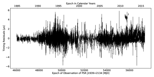
Figure 1: $31$ years of timing residuals of J1939 along with error bars, after removal of timing noise, which is estimated by TEMPO2 using $100$ noise harmonics, as explained later in the text.

Finally, the BAT are modeled using the following parameters: (1) the position of the pulsar in the sky (right ascension $\alpha$ and declination $\delta$), (2) its proper motion ($\mu_{\alpha}$ and $\mu_{\delta}$), (3) its parallax ($\pi$) and (4) fine correction to the DM, if the data permits their modeling, (5) the pulsar’s rotation frequency and its derivative with respect to time ($\nu$ and $d\nu/dt=\dot{\nu}$; for J1939 the second frequency derivative $\ddot{\nu}$ is not used as explained later). The time difference between the observed and modeled BAT are known as timing residuals. In J1939 these residuals represent what is known as timing noise (also known as “red” noise, implying low frequency variation of timing residuals). The main effort of this work is to obtain the timing noise of J1939. After removal of timing noise, the timing residuals should ideally reflect random and uncorrelated noise (mainly instrumental), also known as “white” noise. This is shown in Figure 1, where the rms of the residuals is $\approx 0.5$ $\mu$s. Even if the operative value is $3$ times larger, a variation of $\approx 1.5$ $\mu$s over $31$ years implies that J1939’s clock is stable at the level of almost one part in $10^{15}$. This is consistent with the value of one part in $10^{14}$ obtained by KTR over about $8$ years of observation.

This brief summary of the technique of pulsar timing ignores several details.

First, the total data consists of about $22$ years of data obtained by European and Australian radio observatories, and about $19$ years of data obtained by North American radio observatories. The former are known as European Pulsar Timing Array (EPTA) data and the Parkes Pulsar Timing Array (PPTA) data. Due to instrumentation and methodology differences, the earlier $\approx 8$ years of the data from the North American radio observatories are combined with the EPTA and PPTA data to form what is known as the International Pulsar Timing Array (IPTA) data. The remaining about $11$ years of the data are known as the NANOGrav data. Further, the IPTA (Verbiest et al, 2016) and NANOGrav (Arzoumanian et al, 2018) data of J1939 are obtained by four European and one Australian, and two North American, radio telescopes, respectively. Each of these observed J1939 for different durations over the last $\approx 31$ years, with different front-end/back-end combinations known as sub-systems, that changed over time as better sub-systems were installed over time. Now, data of any two sub-systems will have a relative instrumental delay, usually in the range of $\mu$s to ms, which has to be estimated and corrected before the two data can be combined. There are totally $36$ sub-systems in the J1939 data, so $35$ instrumental delays have to be estimated to align the whole data set. This is not easy as data of different sub-systems often either do not overlap in epoch, or overlap minimally.

Next, reliable estimation of DM of J1939 requires nearly simultaneous observations at two or more radio frequency bands, since the DM changes with epoch; this is often not achieved. The best data in this regard was obtained by KTR in which the dual frequency observations were typically separated by about $1$ hour. Often this can be as large as days or even weeks in the rest of the data. Therefore for some duration, the DM has to be modeled (like the other $7$ pulsar parameters) as a function of epoch, instead of being directly estimated (which is done using equation $4$ of KTR).

Finally, while modeling the BAT to estimate the various pulsar parameters, the presence of “red” timing noise introduces correlations between adjacent timing residuals; the correlation length depends upon the “redness” of the timing noise. This has to be accounted for in the linear weighted least squares parameter estimation algorithm (Coles et al, 2011; Caballero et al, 2016).

The IPTA (Verbiest et al, 2016) and NANOGrav (Arzoumanian et al, 2015, 2018) groups analyzed the J1939 data separately, since the two data contain a fundamental difference, using different methods of DM estimation, correction for “red” noise correlation, etc.

1.2 Incompatibility of IPTA and NANOGrav Data

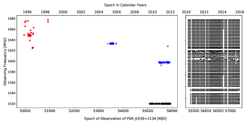
Figure 2: Illustration of incompatibility between IPTA and NANOGrav data, using the $1600$ MHz L-band data. The left panel plots the radio frequency of observation of the IPTA data from Parkes (dots), Jodrell Bank (+) and Nancay (*) Observatories. The right panel displays the NANOGrav data from the Green Bank Observatory that corresponds to the same frequency range as that in the left panel, although the actual frequency range of this data is from $1100$ MHz to $1900$ MHz.

The left panel of Figure 2 shows the exact observational radio frequency used to obtain each SAT, as a function of epoch, for three observatories of IPTA, viz., the Parkes, Jodrell Bank and Nancay observatories; the observations were done at around $1600$ MHz in the L-band. The Parkes data lies at frequency $\approx 1650$ MHz, below MJD $51000$; the Jodrell data is clustered almost exactly at frequency $1520$ MHz, at MJD between $55000$ and $56000$; the rest of the data in the left panel is from Nancay. The Jodrell and Nancay data are obtained within a relatively narrow band of frequencies around the central frequency. The central frequency of the Nancay data changes slightly between the earlier and later epochs, ignoring two points which appear to be outliers. The Parkes data is more spread out in frequency, but still within a band of $\pm 30$MHz around the central frequency. Moreover, the IPTA data consists of just one SAT at each epoch of observation.

In contrast, the NANOGrav data from Green Bank Observatory in the right panel is spread over a band of about $160$ MHz. Moreover, the NANOGrav data consists of several tens of SAT (sometimes as large as $50$) at each epoch of observation. This is because of the extremely wide (radio) band sub-systems used at the Green Bank Observatory. Since the IPTA and NANOGrav data overlap in epoch, they have been plotted in separate panels in Figure 2 for clarity. The situation depicted in this figure holds true for the data in other radio frequency bands as well.

Now, it is well known that the integrated profile of pulsars is radio frequency dependent, and usually becomes narrow at higher frequencies (Manchester & Taylor, 1977). This would cause an additional frequency dependent delay in the SAT, that is not DM related. This aspect can be ignored when the observing bandwidth is narrow (IPTA data), but can not be for wide-band sub-systems (NANOGrav data). The NANOGrav group has dealt with this issue by introducing what are known as “FD” parameters into their analysis; see section $4.2$ of (Arzoumanian et al, 2015). Now, using the FD parameters for the IPTA data would distort the timing residuals. Therefore there is a fundamental issue involved in combining the IPTA and NANOGrav data for analysis.

Verbiest et al (2016) combine such data for other pulsars, and discuss the problems involved, but not in the manner described here; see particularly their sections $1.4$, $2.2$ and $3.1$.

1.3 The Current Work

This work combines the two data sets by selecting only a few SAT per epoch of the NANOGrav data, such that they lie within a narrow radio bandwidth, and also such that their spread in the time domain is less than $1$ $\mu$s. This eliminates the need for the FD parameters. Tests show that this number can be as low as one SAT per epoch, mainly on account of the excellent quality of the NANOGrav data.

Section $2$ describes the observations and the procedure of analysis, including data selection and estimation of the DM. Section $3$ presents the results of analyzing the data in four independent ways, while section $4$ discusses the results.

2 Observations and Analysis

Figure 3 summarizes the available data of J1939. Each point represents an observation of either single or multiple SAT at that epoch. Each horizontal track represents data of one sub-system, indicating both the total duration of observation, as well as the cadence of observation in that duration. The bottom $7$ tracks belong to the UHF band, the middle $20$ belong to the L-band, and the top $9$ belong to the S-band; space is provided between bands for clarity. For further clarity, the $16$ tracks at frequency $\approx 1400$ MHz in the L-band are separated by space from the $4$ tracks at frequency $\approx 1600$ MHz in the same band. The left ordinate is labeled by the observatory or radio telescope concerned, and the average statistical error of the SAT of that track (in $\mu$s). The right ordinate is labeled by the symbol used for the observing sub-system by the original observers, and their relative instrumental offsets in $\mu$s.

The four L-band tracks at $1600$ MHz are expanded in frequency in Figure 2, except for that of the Parkes Telescope (PKS) sub-system “fptm.20cm-legacy”, which consists of both $1400$ and $1600$ MHz data; so only the latter part has been used in Figure 2.

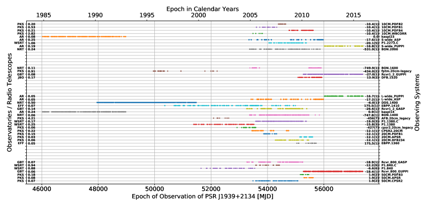
Figure 3: Summary of IPTA and NANOGrav observations of J1939 that are available in the public domain. The first column of labels of the left ordinate are: (1) AR = Arecibo Telescope, (2) EFF = Effelsberg Telescope, (3) GBT = Green Bank Telescope, (4) JBO = Jodrell Bank Observatory, (5) NRT = Nancay Radio Telescope, (6) PKS = Parkes Telescope, and (7) WSRT = Westerbork Synthesis Radio Telescope. The second column of labels are the average error on the SAT in $\mu$s. The first column of labels of the right ordinate are the instrumental offsets (in $\mu$s) for each sub-system, with respect to that of “kaspi23”; the error in the last digit is given in parenthesis. The second column of labels of the right ordinate represent sub-systems. Some important references for this table are: Arzoumanian et al (2015, 2018); Backer et al (1982); Cordes et al (1990); Hotan et al (2006); Kaspi, Taylor & Ryba (1994); Manchester et al (2013); Ramachandran et al (2006); Shannon & Cordes (2010); Verbiest et al (2009, 2016), and references therein.

The earliest observations of J1939 are those of KTR using the Arecibo Telescope (AR) (sub-systems kaspi14 and kaspi23 in the L and S bands; see the caption of Figure 3 for observatory abbreviations). Then Nancay Radio Telescope (NRT) started observing in just the L-band using an older sub-system (DDS.1400). This provided relatively lower quality data, but it was their first sub-system, and provided crucial overlap with the data of KTR; their later sub-systems provided data as good as any other sub-system. Then the Effelsberg Telescope (EFF) started observations with overlap with the data of NRT. Their duration of observation was one of the longest, although there were gaps in the observations; and their data quality is one of the best; unfortunately theirs was also a single frequency observation (L-band). Since after the year $2011$ it appears that data of J1939 is being provided by only the North American telescopes.

Figure 3 shows the inhomogeneity of the data of J1939, in terms of duration of observation, the cadence of observation within any duration, and the quality of the data. It also shows that for about $7$ years after MJD $49000$, there were no multi-frequency observations available in the public domain that could be used to estimate the DM.

2.1 Data Selection

The rationale of data selection can be understood using Figure 4. The narrow band sub-system Rcvr1_2_GASP of Green Bank Telescope (GBT), of bandwidth of about $50$ MHz, was replaced by the broad band sub-system Rcvr1_2_GUPPI, of bandwidth of about $740$ MHz, towards the end of the year $2010$. Because of frequency evolution, the pulse of J1939 arrives at different times at different frequencies within the band of observation, even after removing the effects of DM. Ideally one should have a unique template integrated profile at each frequency for obtaining the SAT at that frequency, but this is too humongous a task. Therefore the integrated profile at a reference frequency within the band of observation is used as the template for the entire band. Now it turns out that the frequency evolution of the pulse profile is negligible for the narrow band sub-system, while it is significant for the broad band sub-system.

If the broad band sub-system was not installed, and the narrow band sub-system had continued observing J1939, then the problem of frequency evolution would not have arisen. In this work such a hypothetical scenario is created, by using from the broad band sub-system, only that data that corresponds to the range of frequencies of the narrow band sub-system. There are several ways of doing this, and this work adopts one of those.

This implies that one would be excising most of the broad band data. This is justified because an observation using a wider band improves the signal to noise ratio of the integrated profile only if the pulses arrive at the same time all over the band, which is not the case here. This work demonstrates that the large collecting areas of the GBT and AR telescopes ensure that there is sufficient signal to noise ratio of the integrated profile within the retained narrow band, to obtain a statistically significant SAT. This scheme will probably not work with wide band data from smaller radio telescopes.

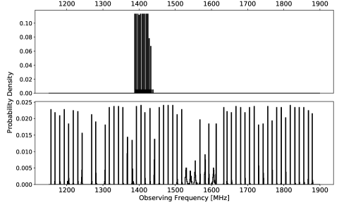
Figure 4: Probability distribution of frequency of observation for the Rcvr1_2_GASP (top panel) and Rcvr1_2_GUPPI (bottom panel) sub-systems, respectively.

The data selected for analysis in this work consists of the entire IPTA data, and part of the NANOGrav data, which was selected as follows. The NANOGrav data itself consists of two relatively narrow band sub-systems labeled ASP and GASP, and two very broad band sub-systems labeled PUPPI and GUPPI; ASP and PUPPI are the back-ends used at the AR telescope, while GASP and GUPPI are identical back-ends used at the GBT. The mean radio frequency of the data of ASP and GASP systems in the UHF, L-band and S-band are $844$, $1410$ and $2352$ MHz, respectively. At each epoch of observation, say $n$ SAT were selected from the multiple SAT available, that were closest in frequency to any of the above three values. For small values of $n$ the selected SAT would have very narrow spread in frequency, and would have very small systematic spread in time due to frequency evolution of the pulse of J1939; for large $n$ the situation would be the opposite. In either case the $n$ SAT would have a mean frequency very close to one of the above three values. Several values of $n$ were tried, and values between $1$ and $10$ were found to be useful. Even $n=1$ served the essential purpose, presumably because of the excellent quality of NANOGrav data. However $n=7$ to $10$ were found to be better for DM estimation; therefore $n=10$ was finally chosen. Larger $n$ caused the systematic spread in time of the SAT to be larger than $1$ $\mu$s. This selection reduced the total data from $18122$ to $6994$ SAT.

In summary, frequency evolution of the pulse essentially converts a broad band observation of J1939 into several narrow band observations that are each observing, in effect, a slightly different pulsar, of which one has been chosen in this work.

2.2 Estimation of DM

The DM of J1939 has to be estimated as a function of epoch to proceed further. The best DM estimate has been done by KTR from MJD about $46000$ to MJD $49000$. From then on until MJD $51650$ only single frequency observations are available in the public domain. However, Ramachandran et al (2006) used additional data, obtained at several frequencies using the NRAO $85$ and $140$ foot telescopes at the Green Bank Observatory, to extend the DM measurements to slightly beyond calendar year $2004$. While this additional data of J1939 are not available in the public domain, the DM results are available in Figure $6$ of Ramachandran et al (2006), and also in Figure $6.6$ of Demorest (2007), from which they were digitized. Next one has to estimate the DM of J1939 for the rest of the data, and align it with the above digitized curve.

The ideal method of estimating the DM at any epoch is to measure the SAT at two well separated frequencies simultaneously, and then to apply equation $4$ of KTR. Such SAT would measure the arrival of exactly the same pulse, but at different frequencies. However this is rarely possible, since changing the front-end of a radio telescope takes time. Therefore the method of KTR is the next best, where the dual frequency observations are separated by about $1$ hour. Since the maximum rate of change of DM of J1939 is about $10^{-5}$ pc cm^-3 per day (as will become evident later), and since the error on the estimated DM is typically larger than $10^{-4}$ pc cm^-3, one can assume that a gap of even $10$ days between multi frequency observations is tolerable for DM estimation of J1939. The IPTA group appears to have used some variation of the KTR method, and have additionally modeled the first and second derivative of DM with respect to epoch. The data gap between NANOGrav observations is much longer, typically $10$ to $14$ days. Therefore they have modeled the DM along with other pulsar parameters (as a function of epoch) using the so called “DMX” parameters.

The approach of this work is to apply the KTR method, allowing for a maximum gap of about $1$ day between multi frequency observations (see Lam et al (2015) for justification). This reduces the number of epochs at which the DM can be estimated, but linear interpolation for the intermediate epochs gives satisfactory results. Equation $4$ of KTR can be re-written as consisting of a term that varies linearly with DM and inversely with the square of the observing frequency, plus a constant term that represents instrumental and other constant delays. Thus for dual frequency data one has to model for two parameters – the DM and one constant relative delay between the two frequencies; for three frequency data one has to model for the DM and two constant relative delays. In this manner the DM as a function of epoch was derived separately for each radio telescope, along with the relative instrumental offsets for the corresponding frequencies. These curves were aligned in the DM space, and the result was then aligned with the digitized DM curve from Demorest (2007).

The TEMPO2 software (Hobbs et al., 2006; Edwards et al., 2006) has been used for most of the analysis of this work.

The DM in this work was estimated by first pruning the data of each telescope, such that only those SAT were retained that had at least one other SAT at another frequency band, that was separated in epoch by less than one day. The reference epoch for the fit (PEPOCH in TEMPO2) was taken to be mid way between the total duration of the pruned data. Now, TEMPO2 provides for inserting time offsets between data sets using the “JUMP” parameter. So JUMP values were inserted for each sub-system within the UHF, S-band and 1600 MHz data of the L-band, with respect to the 1400 MHz data of the L-band data. A constant value of $=71.0270$ pc cm^-3 was used for the DM parameter of TEMPO2. Correlation due to “red” noise was taken into account, but was required only for the WSRT telescope, whose data duration was quite long; for the rest of the telescopes “whitening” of the data was achieved by using the $\ddot{\nu}$ parameter in TEMPO2. Note that this $\ddot{\nu}$ represents the local curvature of the timing data for each telescope – it is not related to the intrinsic $\ddot{\nu}$ of J1939, which is too small to be estimated in our data. Then the residuals of the fit were extracted using the “general2” plugin of TEMPO2. These were then analyzed outside TEMPO2 to estimate the residual DM as a function of epoch, using Equation 4 of KTR. The sum of the residual DM and $71.0270$ results in the final DM as a function of epoch, for each telescope. Note that TEMPO2 has the ability to estimate the instrumental offset of data that do not overlap in epoch, as long as the lack of overlap is not of very long duration, and as long as the data is sufficiently “whitened”.

2.3 Analysis of SAT

A uniform set of TEMPO2 parameters was used for the selected data; the IPTA and NANOGrav groups used different values for these parameters (see Appendix A).

The DM for each SAT was estimated using linear interpolation on the final DM curve obtained in the previous section; this was tagged to each SAT using the TEMPO2 flag “-dmo”, after removing the original DM tag inserted by the IPTA group. No further DM modeling was done in TEMPO2.

Next, the L-band $1400$ MHz data of each telescope was aligned, by estimating the instrumental delays between them, using the method described in the previous section. The instrumental delays of the UHF and S-band data of each telescope, relative to their $1400$ MHz L-band data, that were estimated in the previous section, were then used to align the rest of the data; only minor changes were required in these delay values for final data alignment. Similarly the L-band $1600$ MHz data were also aligned. The IPTA and NANOGrav groups started with initial JUMP values, and then varied them as any other parameter to be fit. This was tried in this work, but better results were obtained by keeping them fixed; so the JUMP values in this work were first estimated as well as possible, and then were held fixed in TEMPO2 (see Appendix A of Arzoumanian et al (2015)). Some observatories have fixed instrumental delays for some SAT, that were included without modification in this work.

Next TEMPO2 is used to derive the values of the parameters of the timing model – $\alpha$, $\delta$, $\mu_{\alpha}$, $\mu_{\delta}$, $\pi$, $\nu$ and $\dot{\nu}$. For J1939 the $\ddot{\nu}$ is expected to be so small (based on the average braking index of a pulsar) that it can not be reliably estimated in this analysis. If the timing residuals after accounting for this model represent “white” noise, then the above parameters would have been estimated in a reliable manner. However, it is known for J1939 that the residuals are slowly varying and sinusoidal (see Figure $5$ of Verbiest et al (2016)). Therefore, the correlation of this “red” noise has to be taken into account for parameter estimation in TEMPO2. This has been done differently by the IPTA and NANOGrav groups.

The IPTA group models this correlation as a specific function, and estimates the three parameters of this function from the data, and inputs these three parameters to TEMPO2 (see Lentati et al (2015) for some details). The NANOGrav group models this correlation as arising from a power law spectrum, and inputs the amplitude and slope of this spectrum to TEMPO2, which then derives $100$ harmonics whose spectrum is (or at least should be) the above power law, and which estimate the timing noise. See section $5.1$ of (Arzoumanian et al, 2015) for details. In this work both methods are used.

The TEMPONEST software (Lentati et al, 2014) was installed, but could not be used on account of prohibitively long run time on my personal computer for $6994$ SAT with “red” noise covariance included. However, the MULTINEST software (Feroz & Hobson, 2008; Feroz, Hobson & Bridges, 2009; Buchner et al, 2014) for Markov Chain Monte Carlo (MCMC) estimation of parameters has been used (Hogg et al, 2010; Hogg, 2012; Hogg & Foreman-Mackey, 2018).

Further details of analysis are given in the following section.

3 Results

3.1 Dispersion Measure of J1939

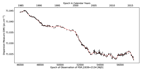
Figure 5: DM of J1939 as a function of epoch for the combined IPTA and NANOGrav data. The earlier DMs have a fixed error of $3\times 10^{-4}$ pc cm^-3, which is explained in the text; the later DMs have estimated errors. The dashed line is a spline curve that best fits the data. The maximum gradient is $10^{-5}$ pc cm^-3 per day.

Figure 5 shows the DM derived for J1939 from the combined IPTA and NANOGrav data. It is almost identical to that of KTR for the first $8$ years, and correlates very well with that of NANOGrav (Arzoumanian et al, 2018) for the last $11$ years. The dashed curve is a smooth representation of the DM data, obtained using the “splinefit” tool of the open source software “octave”. The rms of the residuals between the DM data and the spline curve is $3\times 10^{-4}$ pc cm^-3, which is similar to the uncertainty in aligning the DM data of different telescopes.

The spline curve was used to obtain the phase structure function $D_{\phi}(\tau)$ of DM variations, that is defined in equation $11$ of KTR, using equations A2 and A3 of You et al (2007). The actual DM data can not be used for this purpose because the earlier half of DM data have no error bars available; these are required to subtract a bias in the function $D_{\phi}(\tau)$. The power law index of the spectrum of electron density fluctuations $\beta$ is $3.86\pm 0.04$ using $31$ years of data. This is consistent with the value of $3.874\pm 0.011$ obtained by KTR, who used the first $8$ years of data. Ramachandran et al (2006) obtained a slightly smaller value of $3.66\pm 0.04$ using the first $20$ years of data. It is therefore concluded that phase structure function $D_{\phi}(\tau)$ of DM variations of J1939 is not evolving over the decades.

3.2 Timing Noise of J1939

Both IPTA and NANOGrav groups use what are known as the T2EFAC and T2EQUAD parameters (henceforth T2 parameters), one pair for each sub-system. The former is used to scale the measured uncertainties on the SAT, while the latter is added to them in quadrature. These are used to ensure that the final reduced $\chi^{2}$ obtained by TEMPO2 is close to the expected value of $1$; see section $3.1.2$ of Verbiest et al (2016). In addition the NANOGrav group uses the ECORR (or jitter) parameter, also one for each sub-system, that acts like the T2EQUAD for data spread in frequency (see section $4.2$ of Arzoumanian et al (2014), and section $3$B of van Haasteren et al (2014)). In this work, firstly the ECORR parameter is not used, on account of the data selection discussed above. Next, the analysis was done using both the original values of the T2 parameters (derived by the IPTA and NANOGrav groups), as well as those that were re-estimated here using the “fixData” plugin of TEMPO2. The latter were consistent with the former, although for some sub-systems the values differed significantly.

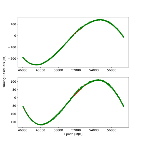
Figure 6: The data in the two panels were obtained using the IPTA (top panel) and the NANOGrav (bottom panel) methods of correction for “red” noise correlation; in both cases re-estimated T2 parameters were used. The dashed line in each panel represents the best fit planetary companion model. The IPTA group models the “red” noise correlation as a specific function with three parameters; these are given in the last three rows of Table 1. The NANOGrav group models the power spectrum of this correlation as a power law, with amplitude and slope of $0.15726$ and $-2.7589$, respectively. TEMPO2 uses these to derive $100$ harmonics which represent the timing noise.

In the following sections the timing noise is modeled as being on account of (1) a planetary companion to J1939, and (2) precession of J1939. In principle the former model can be explored using the binary parameters of TEMPO2. However, this attempt failed due to either (a) converging to negative values of eccentricity of the elliptical orbit, or (b) resulting in very large errors on the binary parameters, both presumably because the data has only one cycle of the orbit. Therefore the results of the following sections are derived by using independent software.

In principle, one can not rule out a third model, viz., that the timing noise could be due random variations in the frequency $\nu$, the variations having a steep power law spectrum. It is argued in later sections that this may not be the case.

3.2.1 Planetary Companion Model

Table 1 summarizes the results of this section while Figure 6 illustrates two of them (columns $3$ and $5$) as plots. In the top panel of Figure 6, the noise model was determined from the data using the “autoSpectralFit” plugin, and input to TEMPO2 using the “-dcf” switch; the parameters of the model (slope $\alpha$, cutoff frequency $f_{c}$, and amplitude $a$) are given in the last three rows of columns $3$ of Table 1. In the bottom panel, the NANOGrav noise model was used – RNAMP $=0.15726$ and RNIDX $=-2.75890$ (see Table $3$ and Figure $3$ of Arzoumanian et al (2015)).

In Figure 6 there is an excess timing noise between MJD $51200$ and $53200$; this coincides with the duration of maximum gradient of DM in Figure 5. These data have been ignored during the curve fit, and will be discussed later.

Table 1: Results of fitting the planetary companion model to the timing noise, that was obtained using both the IPTA (columns $2$, $3$) and the NANOGrav (columns $4$, $5$) methods of correction for “red” noise correlation. In each case, both the original T2 parameters (orig), as well as those re-estimated here (local), were used. $A$ is the projected semi major axis of the orbit, $e$ is its eccentricity and $P$ is the period of orbit. The last three rows of IPTA contain the derived parameters of the noise model – $\alpha$ and $a$ are the exponent and amplitude, while $f_{c}$ is the cut-off frequency. For the NANOGrav noise model, the original RNAMP $=0.15726$ and RNIDX $=-2.7589$ were used.

Method	IPTA		NANOGrav
T2param	$orig$	$local$	$orig$	$local$
$A$ ($\mu$s)	$129.9\pm 0.1$	$197.6\pm 0.1$	$140.6\pm 0.1$	$141.1\pm 0.1$
$e$	$0.219\pm 0.001$	$0.158\pm 0.001$	$0.211\pm 0.001$	$0.215\pm 0.001$
$P$ (days)	$11105\pm 2$	$13068\pm 3$	$11403\pm 2$	$11381\pm 2$
rms ($\mu$s)	$1.5$	$1.0$	$1.2$	$1.2$
$\chi^{2}_{d}$	$35.0$	$30.2$	$24.0$	$39.2$
$\alpha$	$3.016$	$5.098$
$f_{c}$	$0.0322$	$0.0322$
$a$	$6.4\times 10^{-23}$	$9.8\times 10^{-20}$

Table 1 show the results of four different analysis – using the IPTA and the NANOGrav methods of correction for “red” noise correlation, and in each of these, using original T2 parameters as well as re-estimated ones. The timing noise in columns $2$ to $5$ of Table 1 are fit to a planetary companion model. The parameters of the elliptical orbit are: the projected semi major axis of the orbit $A$, its eccentricity $e$ and period of orbit $P$, epoch $T0$ and longitude $\omega$ of periastron; only the important first three parameters are listed in the first three rows of Table 1. The formula for the BAT in this case is well known (for example see Eq. $9$ of Malhotra (1993)). No approximation has been made in fitting the planetary model – the full Kepler equation has been solved. The results of Table 1 have been obtained using the “curve_fit” tool of the Python module “scipy”. Then they have been verified, particularly regarding the distribution of errors and their correlations, using the “solve” tool of the Python implementation of MULTINEST (pymultinest). To speed up this algorithm the critical code was written in C, and called as a library in Python using its C interface.

The parameters of the top and bottom panels of Figure 6 are given in columns $3$ and $5$ of Table 1. $rms$ is the standard deviation of the timing noise after subtraction of the planetary companion model, while $\chi^{2}_{d}$ is the $\chi^{2}$ per degree of freedom of the fit. In all four cases the $\chi^{2}_{d}$ is much higher than $1$, indicating that the formal uncertainties are underestimated even after implementing the T2 parameters. However the $rms$ is less than $1.5$ $\mu$s, which is a small fraction of the total amplitude $A$ of the fit.

The timing residuals in Figure 1 are the difference between the timing noise in column $4$ of Table 1, and the curve represented by the $100$ noise harmonics. this is not the same as subtracting the planetary companion model. The $100$ noise harmonics model fits almost every twist and turn of the timing noise, including the excess timing noise between MJD $51200$ and $53200$.

The NANOGrav analysis yields consistent values of $A\approx 140$ $\mu$s, $e\approx 0.21$ and $P\approx 11400$ days. The IPTA analysis using original T2 parameters is also consistent with the above values (column $2$ of Table 1); only the results in column $3$ are divergent. In the rest of this section the average of the above three values will be adopted, viz., $A=137.2$ $\mu$s, $e=0.215$ and $P=11296$ days.

Using the above $A$ and $P$ values in Eq $2$ of Vivekanand (2017), the mass of the planetary companion is about $3.5\times 10^{-8}$ times the solar mass, which is approximately the mass of the moon. Using Kepler’s third law the semi-major axis of the relative orbit is about $11$ AU (Starovoit & Rodin, 2006).

3.2.2 Precession Model

The model of a freely precessing pulsar can be understood using Figure $3$ of Link & Epstein (2001). The angular momentum and dipole moment vectors of J1939 make the angles $\theta$ and $\chi$ with its symmetry axis, respectively. However since pulsars slow down due to electromagnetic torque, J1939 must be precessing under the influence of a torque. In this scenario the timing residuals are given by:

$$f(t)=k+a_{1}\sin\left(\omega_{p}(t-t_{0})\right)-a_{2}\sin 2\left(\omega_{p}(t-t_{0})\right),$$ (1)

where for small wobble angle $\theta$

$$a_{1}=\frac{\kappa\theta\sin 2\chi}{1+\theta^{2}};a_{2}=\frac{\kappa\theta^{2}\sin^{2}\chi}{4(1+\theta^{2})}.$$ (2)

(Eq. C46 of Akgun et al (2006); see also Eq $13$ of Link & Epstein (2001), and also Jones & Andersson (2001)). $k$ is an arbitrary offset, $a_{1}$ and $a_{2}$ are the amplitudes of the first and second harmonics of the precession frequency $\omega_{p}=2\pi\nu_{p}=2\pi/P$. $\kappa$ is proportional to the strength of the spin down torque of J1939.

Table 2: Results of fitting the precession model to the timing noise; the rest is as in Table 1, except that the last three rows of that table are not repeated here. $a_{1}$ and $a_{2}$ are the amplitudes of the first and second harmonics of period $P$ (see Equation $1$).

Method	IPTA		NANOGrav
T2param	$orig$	$local$	$orig$	$local$
$a_{1}$ ($\mu$s)	$124.4\pm 0.1$	$193.2\pm 0.1$	$135.0\pm 0.1$	$135.2\pm 0.1$
$a_{2}$ ($\mu$s)	$9.9\pm 0.1$	$10.2\pm 0.1$	$11.0\pm 0.1$	$11.2\pm 0.1$
P (days)	$11277\pm 3$	$13475\pm 3$	$11594\pm 3$	$11609\pm 4$
rms ($\mu$s)	$3.4$	$2.5$	$2.9$	$2.9$
$\chi^{2}_{d}$	$174.8$	$104.1$	$141.2$	$225.9$

Table 2 summarizes the results of this section while Figure 7 illustrates two of them (columns $3$ and $5$) as plots. Figure 7 is the same as Figure 6 except that the curve fitted to the timing noise is given in Eq $1$. Only the important last three parameters of Eq $1$ are listed in the first three rows of Table 2.

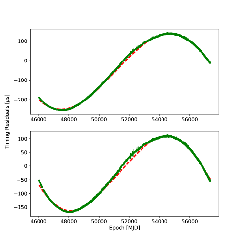
Figure 7: The data is the same as in Figure 6. The dashed line in each panel represents the best fit precession model.

The $\chi^{2}_{d}$ in Table 2 are $\approx 5$ times larger than those in Table 1, while the $rms$ are $\approx 2.5$ times larger. Clearly the data fits the planetary companion model better than the precession model. This is also obvious when comparing the solid curves in Figure 6 and Figure 7. As before, the average of the values in columns $2$, $4$ and $5$ of Table 2 will be used for further analysis, viz., $a_{1}=131.5$ $\mu$s, $a_{2}=10.7$ $\mu$s, $P=11493$ days.

The oblateness of J1939 $\epsilon=(I_{3}-I_{1})/I_{1}$, where $I_{i}$ are the three components of the moment of inertia (for a bi-axial rotator $I_{3}>I_{2}=I_{1}$). Within the approximations used to derive Eq $1$, the oblateness is $\epsilon\approx\omega_{p}/\omega=\nu_{p}/\nu=1/(11493\times 86400)/641.928\approx 1.57\times 10^{-12}$; see also Eq $67$ of Jones & Andersson (2001).

Using Eq $2$ above $\theta\tan\chi=8\times a_{2}/a_{1}=0.65$ radians. Integration of Eq $19$ of Link & Epstein (2001) gives $\theta\tan\chi=2\times a_{2}/a_{1}=0.16$ radians, which is similar to the above result correct to within a factor of $4$. However, using Eq $65$ of Jones & Andersson (2001), $\theta\approx 3\times 10^{-6}\tan\chi$ radians, giving an altogether different functional form. Therefore there is some discrepancy in the values of $\theta$ obtained by the three groups (Akgun et al (2006); Link & Epstein (2001); Jones & Andersson (2001)), although all three formulae are derived under similar approximations. For this work $\theta\tan\chi\approx 0.4$ radians will be assumed. Since $\chi$ in J1939 is supposed to be very close to $90^{\arcdeg}$ (it has an inter pulse), $\theta$ is expected to be a very small value.

3.3 Excess Timing Noise

In Figure 6 the excess timing noise between MJD $51200$ and $53200$ coincides with the duration of maximum gradient of DM of J1939. This manifests as a noisy bump when the fitted curve is subtracted from the data in the two panels in Figure 6. This is an achromatic excess timing noise, so it is independent of the DM. Further, the DM in this duration is very well estimated due to excellent overlap of the digitized DM values and those estimated in this work. Currently the origin of this excess timing noise is unknown.

4 Discussion

Shannon et al (2013) studied the timing noise of J1939 using $26$ years of timing data. They have excluded the possibility of a single object causing these timing results because of “the lack of an obvious periodicity” in their timing residuals; see first line of first para after their Eq. $2$ in their section $2$. This situation does not apply to this work, which has  5 more years of data, and has a clear periodicity. Moreover, Shannon et al (2013) have themselves flagged the most serious drawback of their asteroid belt model, viz., ”that it is difficult, though not impossible, to test”; see first line of their section 7.

Before discussing the planetary companion/precession models, a few technical issues will be highlighted.

In this work, only one cycle of either planetary orbit or precession is available for analysis. This would limit the confidence with which the corresponding parameters can be estimated. Unfortunately, even the second cycle of data is unlikely to be obtained any time soon.

Assuming a braking index of 3, the $\ddot{\nu}$ expected for J1939 is $8.8\times 10^{-30}$ Hz sec^-2. The total duration of observation of $11324$ days would cause $8.8\times 10^{-30}\times(11324*86400)^{3}/6.0=0.0014$ of additional phase across the entire duration, which is about $2.2$ $\mu$s. This is negligible compared to the $\approx 130$ $\mu$s amplitude of the sinusoidal timing noise. So the sinusoids in Figures 6 and 7 are not an artifact of the cubic term.

The fact that the period of the timing noise lies very close to the total duration of observation could cause some concern. However, there appear to be no known artifacts in TEMPO2 (or in any other software/algorithm that is used here) that might mimic a periodicity of the order of the length of the data used. This issue is discussed in greater detail in the Appendix.

Why does the MCMC algorithm produce much smaller errors than TEMPO2? I believe it is because the MCMC planetary companion modeling involves a non-linear fit to an exact ellipse, while the TEMPO2 binary fit involves a linear fit to an approximate ellipse (an ellipse that has been linearized with respect to its parameters). Two binary models (BT and DD) were tried within TEMPO2, and both failed to converge most of the time. Convergence occurred when the initial values were almost the converged values, but the errors on the parameters were larger; here many more cycles of the sinusoid in the data would have helped. This issue is discussed in greater detail in the Appendix.

Now, the important question concerning the planetary companion of J1939 is – how did it form around a millisecond pulsar (MSP)? Phillips & Thorsett (1994) summarize the various possibilities. In a few of these, the planet is formed before the neutron star (NS) is formed, and somehow survives the supernova explosion (SNE); but in most of them the planet is formed after the NS.

In the former scenarios, a planet that is formed around a normal star, and that survives the passage through the expanding Red Giant envelope of the star, would still become unbound after the SNE since more than half the mass of the system might be lost to the ISM. This can be avoided only if the SNE is asymmetric and preferentially oriented with respect to the velocity of the planet, or alternately, if the planet’s orbit is highly eccentric. In either case, this scenario may work for a slow pulsar but not for a MSP, which has to be spun up to ms periods by accretion from a companion star. Another possibility is that the planet formed around a system of normal binary stars, one of which underwent a SNE, which did not disrupt the binary because less than half the mass of the system got expelled into the ISM, and later the NS spiraled into the companion star. Finally the simplest scenario, but statistically the least probable, would be the capture of a planet around a normal star by a MSP in a chance exchange interaction (see references in Phillips & Thorsett (1994)).

In the latter scenarios, the planet is formed from the disk material around the MSP. But to spin a NS to ms periods one requires mass accretion from a companion star, which must somehow be gotten rid of later, leaving just the disk material. One mechanism of doing this is through evaporation of the star by the pulsar wind; some of the evaporated material forms the disk from which the planet can form. This mechanism is expected to form planets that are approximately Moon size, so this scenario appears to be a possibility in J1939. Yet another scenario is that the companion of the NS is a white dwarf (WD), and the mass losing WD is reduced to a disk (see references in Phillips & Thorsett (1994)).

While it is not clear which of these various possibilities (and the several more summarized by Phillips & Thorsett (1994)) explain the case of J1939, this work places the following constraints: (1) the planet around MSP J1939 is at a distance of $11$ AU, which is similar to the distance of $10.26$ AU of the planet around the slow pulsar B0329+54 (Starovoit & Rodin, 2006), and much larger than the distances of $0.36$ and $0.47$ AU of the two planets around the MSP B1257+12 (Wolszczan & Frail, 1992); (2) its eccentricity $e=0.21$ is similar to that of the planet around B0329+54 ($0.24$), while the eccentricities of the two planets of B1257+12 are almost negligible ($\approx 0.02$); and (3) the masses of the three planets mentioned above are $2$, $3.4$ and $2.8$ Earth masses, respectively, while the planet around J1939 is about $100$ times less massive. Thus, while J1939 shares an evolutionary scenario with the ms PSR B1257+12 in terms of mass accretion, its planetary distance and eccentricity appear to be similar to that of the slow PSR B0329+54, whose evolution is entirely different. As an illustration of the constraints, theories of planet formation around B1257+12 have to invoke mechanisms to circularize the planets’ orbits, either during their formation or later, while theories of planet formation around J1939 must suppress the very same mechanisms, while starting off with the common scenario of mass accretion that is mandatory for MSPs.

Now coming to the precession model of J1939, in this work precession under the influence of the electromagnetic torque of the pulsar is considered, not free precession. The main difference between the two cases is (1) the timing noise would be strictly a sine wave in the latter case, while it will have a second harmonic in the former case; and (2) the amplitude of the sine wave will be significantly enhanced when torque drives the precession, even if the oblateness $\epsilon$ is very small (Jones & Andersson, 2001; Link & Epstein, 2001; Akgun et al, 2006).

Next, the shape of J1939 is assumed to be bi-axial for which two of the moments of inertia are equal. However, given the very small value of $\epsilon$ estimated in this work, one should also explore the tri-axial case ($I_{3}>I_{2}>I_{1}$). Akgun et al (2006) have derived formulae for the timing noise in this case, which are very complicated, and whose application is beyond the scope of this work.

The oblateness J1939 is $\epsilon\approx 1.57\times 10^{-12}$; in comparison, the value for the Crab pulsar is (assuming that it precesses) $\epsilon\approx 6.27\times 10^{-10}$, for PSR B1642-03 it is $\epsilon\approx 4.48\times 10^{-9}$ Jones & Andersson (2001). The latter two pulsars are not MSPs, so it is interesting to speculate if the very low oblateness of J1939 has something to do with its being recycled due to accretion. Could this process have kept the surface of J1939 very hot for so long that the NS adjusted to a new equilibrium shape having very low oblateness? Here it should be noted that there are two contributions to the oblateness – a centrifugal deformation due to the very high rotation of J1939, and Coulomb deformation due to the rigidity of its crust. Precession depends only upon the latter (see section $3$ of Link & Epstein (2001)). Thus the very low $\epsilon$ of J1939 would imply that its Coulomb crust is not at all strained (see section $6$ of Link & Epstein (2001)).

Precession in J1939 can be damped if its crust couples to the interior super fluid, on time scales of $2\pi\tau_{f}\nu$ precession periods, where $\tau_{f}$ is the coupling time scale and $\nu$ is the rotation frequency of J1939 (see section $3$ of Link & Epstein (2001)). Since it is not damped in J1939 for $31$ years, it implies that the crust of J1939 is essentially decoupled from its super fluid interior. This would imply that either super fluid vortices do not pin to the crust of J1939, or its precession is strong enough to break the pinning. Either way one would not expect to see timing glitches in J1939, since that involves sudden unpinning of pinned vortices (Alpar et al, 1984).

That J1939 has displayed no glitches so far is consistent with the belief that pinning of super fluid vortices suppresses precession in pulsars (Shaham, 1977).

Finally, the method of combining the IPTA and NANOGrav data adopted here might prove useful to PTAs in extending their search to lower spatial frequencies.

The treatment of red noise in this paper can probably be done in an alternate way using modern statistical techniques such as ARMA, ARIMA, ARFIMA, GARCH (Feigelson et al., 2018).

5 Appendix

5.1 TEMPO2 Usage

Table 3: Some TEMPO2 parameters used by IPTA, NANOGrav and this work.

PARAMETER	IPTA	NANOGrav	THIS WORK
NE_SW	$4.0$	$0.0$	$4.0$
EPHVER	$5$		$5$
EPHEM	DE421	DE436	DE436
CLK	TT(BIPM2013)	TT(BIPM2015)	TT(BIPM2015)
UNITS	TCB	TDB	TCB
TIMEEPH	IF99	FB90	IF99
T2CMETHOD	IAU2000B	TEMPO	IAU2000B
DILATEFREQ	Y	N	Y
PLANET_SHAPIRO	Y	N	Y
CORRECT_TROPOSPHERE	Y	N	Y

Table 3 shows some important parameters of the TEMPO2 runtime environment that differ for the IPTA and the NANOGrav groups. The NANOGrav group uses a more modern planetary ephemeris (EPHEM) and a more modern realization of the Terrestrial Time (CLK). However, the NANOGrav group uses an older method of transforming the observatory coordinates to the celestial frame for “Roemer” delay (T2CMETHOD), an older method of conversion from SAT to BAT (UNITS), and also an older method of estimating the “Einstein” delay (TIMEEPH). They also do not apply gravitational red shift and time dilation to observing frequency (DILATEFREQ), do not apply tropospheric delay corrections (CORRECT_TROPOSPHERE), and do not compute Shapiro delay due to the planets in the solar system (PLANET_SHAPIRO). Finally, they do not compute the dispersion delay in the solar system due to the solar wind; they set the solar electron density (at $1$ AU) to zero (NE_SW).

5.2 Timing Noise

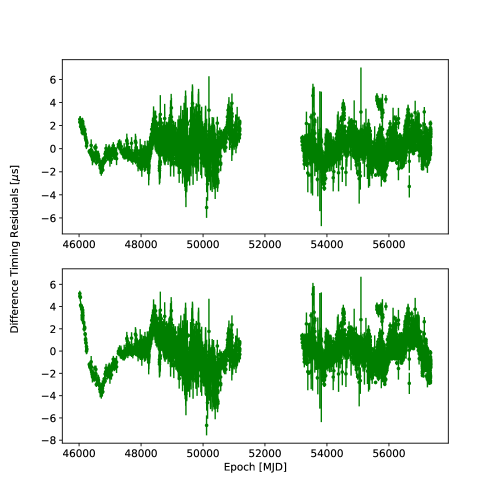
Figure 8: Difference between the data and the modeled curves of Figure 6.

Figure 6 shows the timing residuals fit to a planetary companion model using the IPTA (top panel) and the NANOGrav (bottom panel) methods of correction for “red” noise correlation. The green curves are the data while the red dashed curves represent the planetary model. Figure 8 shows the corresponding plots after subtracting the model from the data; the excess timing noise between MJD 51200 and 53200 has been ignored. The standard deviations of the difference timing residuals in the top and bottom panels of Figure 8 are $1.0$ $\mu$s and $1.2$ $\mu$s, respectively, both of which are comparable to the value $0.5$ $\mu$s estimated in Figure 1. In both panels of Figure 8 the fit appears to be poor only in the initial $1000$ days of the data; for the rest of the data the differences are flat within errors. Therefore one concludes that the planetary companion model is a genuine representation of the timing residuals of J1939.

Figure 9 shows difference timing residuals of the data in Figure 7, in which a precession model has been fit. The standard deviations of the difference timing residuals in the top and bottom panels of this figure are $2.5$ $\mu$s and $2.9$ $\mu$s, respectively. These are significantly higher than those in Figure 8; the fit is poor over the first half of the data. This supports the contention in the paper that the planetary model is a better fit to the timing residuals of J1939 than the precession model. However the latter can not be ruled out entirely since it does fit the later half of the data in the top panel of Figure 7, the standard deviation of the fit for this data being $1.2$ $\mu$s.

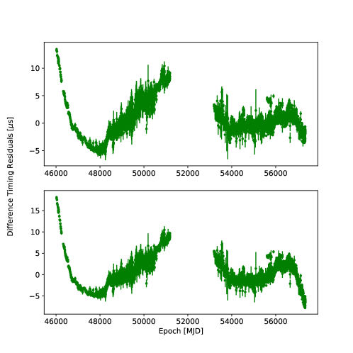
Figure 9: Difference between the data and the modeled curves of Figure 7.

An important issue concerns the spread in period ($P$) values in Tables $1$ and $2$. The mean value of the periods of the four planetary orbits in Table 1 is $11739$ days, while their standard deviation is $2.1$ years, which is significantly larger than the formal errors on the periods, which are of the order of a few days. These are clearly due to uncertainties in the red noise models as well as the choice of the T2 parameters. From a practical point of view the larger uncertainty should be used in understanding the period of the planetary orbits. Similarly, the mean and standard deviation of the periods of the four precession models in Table 2 are $11989$ days and $2.4$ years, respectively.

As mentioned in the text, the large values of reduced $\chi^{2}$ in Tables $1$ and $2$ reflect the fact that the use of the T2 parameters is of limited utility for the data of J1939. In any case such large values of reduced $\chi^{2}$ should not be a surprise when combining highly disparate data from $36$ different sub-systems.

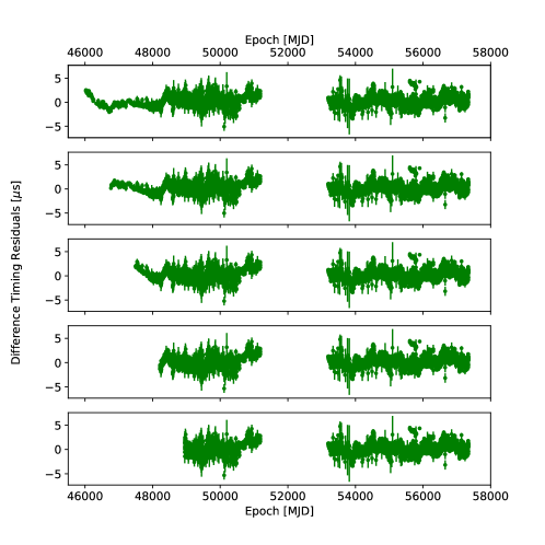
Figure 10: Difference between the data and the modeled curves of top panel of Figure 6. Top panel: Same as the top panel of Figure 6. Subsequent panels: Each panel has two years of data less than the previous panel.

Finally, it is relevant to ask if there are correlations between the length of data used and the periodicities derived, in Figure 6. This might be the case if the timing residuals were due to random variations in the frequency $\nu$, the variations having a steep power law spectrum. The top panel of Figure 10 is exactly the same as the top panel of Figure 8; this is for better comparison with the rest of the panels of Figure 10. The second panel (from the top) in Figure 10 is the same, but with the first two years of data excised; the next panel has the first four years of data excised; the last two panels have the first six and eight years of data excised, respectively. The planetary model fits the smaller amount of data equally well. The corresponding derived parameters are given in Table 4.

Table 4: Results of fitting the planetary companion model to the timing noise, using the IPTA methods of correction for “red” noise correlation, and using local T2 parameters. The second column of this table is identical to the third column of Table 1. Columns three on wards display the parameters obtained when decreasing amount of data is used for the fit; the number of years of data excised from the starting epoch is displayed at the head of each column.

Method = IPTA		T2param = local
	$0$ yr	$2$ yr	$4$ yr	$6$ yr	$8$ yr
$A$ ($\mu$s)	$197.6\pm 0.1$	$197.8\pm 0.1$	$198.8\pm 0.1$	$199.3\pm 0.2$	$200.0\pm 0.7$
$e$	$0.158\pm 0.001$	$0.152\pm 0.001$	$0.147\pm 0.001$	$0.145\pm 0.001$	$0.145\pm 0.01$
$P$ (days)	$13068\pm 3$	$13139\pm 6$	$13276\pm 13$	$13337\pm 21$	$13370\pm 51$
rms ($\mu$s)	$1.0$	$1.0$	$1.0$	$1.0$	$1.0$
$\chi^{2}_{d}$	$30.2$	$29.5$	$29.1$	$29.8$	$32.5$

Columns two to six of Table 4 correspond to the best fit parameters of panels one to five of Figure 10, respectively. Column two of this table is identical to column three of Table 1. Columns three to six of Table 4 have two, four, six and eight years of initial data excised before fitting the planetary companion model. It is clear that the excised data produces results that are consistent with the complete data. The rms in columns three to six are almost the same (up to the first decimal place) as the rms in column 2. So are the $\chi^{2}$ per degree of freedom. The parameters $A$, $e$ and $P$ in columns three to six of Table 4 are also almost similar to those in column two, with a tendency to have larger formal errors when more data is excised. Therefore there appears to be no correlation of the derived periods $P$ with the length of the data used for the planetary model. This is reflected in the almost similar difference timing residuals in the panels of Figure 10 for the data that is common across panels.

References

- Akgun et al (2006) Akgun, T., Link B., & Wasserman I . 2006, MNRAS, 365, 653
- Alpar et al (1984) Alpar, M.A., Anderson, P.W., Pines, D. & Shaham, J. 1984, ApJ, 276, 325
- Arzoumanian et al (2014) Arzoumanian, Z., Brazier, A., Burke-Spolaor, S. 2014, ApJ, 794, 141
- Arzoumanian et al (2015) Arzoumanian, Z., Brazier, A., Burke-Spolaor, S. 2015, ApJ, 813, 65
- Arzoumanian et al (2018) Arzoumanian, Z., Brazier, A., Burke-Spolaor, S. 2018, ApJS, 235, 37
- Backer et al (1982) Backer D.C., Kulkarni S.R., Heiles C., Davis M.M., Goss W.M., 1982, Nature, 300, 615
- Backer & Hellings (1986) Backer, D. C. and Hellings, R. W. 1986, ARA&A, 24, 537
- Buchner et al (2014) Buchner, J., Georgakakis, A., Nandra, K., et al 2014, A&A, 564, A125
- Caballero et al (2016) Caballero, R.N., Lee, K.J., Lentati, L. et al 2016, MNRAS, 457, 4421
- Coles et al (2011) Coles, W,. Hobbs, G., Champion, D.J., Manchester, R.N., & J. P. W. Verbiest, J.P.W. 2011, MNRAS, 418, 561
- Cordes et al (1990) Cordes J.M., Wolszczan A., Dewey R.J., Blaskiewicz M., Stinebring D.R., 1990, ApJ, 349, 245
- Demorest (2007) Demorest, P.B. 2007, Ph. D. Thesis, Univ. of California, Berkeley
- Edwards et al. (2006) Edwards, R.T., Hobbs, G. B., and Manchester, R. N. 2006, MNRAS, 372, 1549
- Feigelson et al. (2018) Feigelson, E.D., Jogesh Babu, G., Caceres, G.A. 2018, Frontiers of Physics, Article 80
- Feroz & Hobson (2008) Feroz F., Hobson M.P. 2008, MNRAS, 384, 449
- Feroz, Hobson & Bridges (2009) Feroz F., Hobson M.P., Bridges M. 2009, MNRAS, 398, 1601
- Hobbs et al. (2006) Hobbs, G. B., Edwards, R.T. and Manchester, R. N. 2006, MNRAS, 369, 655
- Hogg et al (2010) Hogg, D.W., Bovy, J., Lang, D. 2010, arXiv:1008.4686
- Hogg (2012) Hogg, D.W. 2012, arXiv:1205.4446
- Hogg & Foreman-Mackey (2018) Hogg, D.W., Foreman-Mackey, D. 2017, ApJS, 236, 11
- Hotan et al (2006) Hotan A.W., Bailes M., Ord S.M., 2006, MNRAS, 369, 1502
- Jones & Andersson (2001) Jones, D.I., Andersson, N. 2001, MNRAS, 324, 811
- Jones et al (2001) Jones, E., Oliphant, E., Peterson, P. et al 2001, SciPy: Open Source Scientific Tools for Python
- Kaspi, Taylor & Ryba (1994) Kaspi, V.M., Taylor, J.H. & Ryba, M.F. 1994, ApJ, 428, 713 (KTR)
- Lam et al (2015) Lam, M.T., Cordes, J.M., Chatterjee, S., & Dolch, T. 2015, ApJ, 801, 130
- Lentati et al (2014) Lentati, L., Alexander, P., Hobson, M.P. et al 2014, MNRAS, 437, 3004
- Lentati et al (2015) Lentati, L., Taylor, S.R., Mingarelli, C.M.F. et al 2015, MNRAS, 435, 2576
- Link & Epstein (2001) Link, B., Epstein, R.I. 2001, ApJ, 556, 392
- Lyne & Smith (2006) Lyne, A. G., and Graham Smith, F. 2006, Pulsar Astronomy, Cambridge Astrophysics
- Malhotra (1993) Malhotra, R., in “Planets Around Pulsars”, ASP Conference Series, Vol 36, pp 89, 1993, Eds J.A. Philips, J.E. Thorsett and S.R. Kulkarni
- Manchester & Taylor (1977) Manchester, R. N. and Taylor, J. H. 1977, Pulsars, W. H. Freeman
- Manchester et al (2013) Manchester R.N., Hobbs G., Bailes M. et al 2013, Publ. Astron. Soc. Aust., 30, 17
- Phillips & Thorsett (1994) Phillips, J.A. & Thorsett, S.E. 1994, Astrophysics and Space Science, 212, 91
- Ramachandran et al (2006) Ramachandran, R., Demorest, P., Backer, D.C., et al 2006, ApJ, 645, 303
- Shaham (1977) Shaham, J. 1977, ApJ, 214, 251
- Shannon & Cordes (2010) Shannon, R.M., Cordes, J.M. 2010, ApJ, 725, 1607
- Shannon et al (2013) Shannon, R.M., Cordes, J.M., Metcalfe, T.S. et al 2013, ApJ, 766, 5
- Starovoit & Rodin (2006) Starovoit, E.D. & Rodin, A.E. 2017, Astronomy Reports, 61, 948
- van Haasteren et al (2014) van Haasteren, R. & Vallisneri, M. 2014, PHYSICAL REVIEW D 90, 104012
- Verbiest et al (2009) Verbiest, J.P.W., Bailes, M., Coles, W.A., et al 2009, MNRAS, 400, 951
- Verbiest et al (2016) Verbiest, J.P.W., Lentati, L., Hobbs, G., et al 2016, MNRAS, 458, 1267
- Vivekanand (2017) Vivekanand, M. 2017, arXiv:1710.05293
- Wolszczan & Frail (1992) Wolszczan, A. & Frail, D.A. 1992, Nature, 355, 145
- You et al (2007) You, X.P., Hobbs, G., Coles, W.A., et al 2007, MNRAS, 378, 493