Forecasts of cosmological constraints from HI intensity mapping with FAST, BINGO & SKA-I

Abstract

We forecast the cosmological constraints of the neutral hydrogen (HI) intensity mapping (IM) technique with radio telescopes by assuming 1-year of observational time. The current and future radio telescopes we consider here are FAST (Five hundred meter Aperture Spherical Telescope), BINGO (Baryon acoustic oscillations In Neutral Gas Observations), and SKA-I (Square Kilometre Array phase I) single-dish experiment. We also forecast the combined constraints of the three radio telescopes with Planck. We find that, the $1\sigma$ errors of $(w_{0},w_{a})$ for BINGO, FAST and SKA-I with respect to the fiducial values are respectively, $(0.9293,3.5792),(0.4083,1.5878),(0.3158,0.4622)$. This is equivalent to $(56.04\%,55.64\%)$ and $(66.02\%,87.09\%)$ improvements in constraining $(w_{0},w_{a})$ for FAST and SKA-I relative to BINGO. Simulations further show that SKA-I will put more stringent constraints than both FAST and BINGO when each of the experiment is combined with Planck measurement. The $1\sigma$ errors for $(w_{0},w_{a})$, BINGO + Planck, FAST + Planck and SKA-I + Planck covariance matrices are respectively, $(0.0832,0.3520),(0.0791,0.3313),(0.0678,0.2679)$, implying $(w_{0},w_{a})$ constraints improvement of $(4.93\%,5.88\%)$ for FAST + Planck relative to BINGO + Planck and an improvement of $(18.51\%,23.89\%)$ in constraining $(w_{0},w_{a})$ for SKA-I + Planck relative to BINGO + Planck. We also compared the performance of Planck data plus each single-dish experiment relative to Planck alone, and find that the reduction in $(w_{0},w_{a})$ $1\sigma$ errors for each experiment plus Planck, respectively, imply the $(w_{0},w_{a})$ constraints improvement of $(22.96\%,8.45\%),(26.76\%,13.84\%)$ and $(37.22\%,30.33\%)$ for BINGO + Planck, FAST + Planck and SKA-I + Planck relative to Planck alone. For the $9$ cosmological parameters in consideration, we find that, there is a trade-off between SKA-I and FAST in constraining cosmological parameters, with each experiment being more superior in constraining a particular set of parameters.

1 Introduction

Cosmology has unveiled our understanding of the universe that has increasingly matured over the last few decades. Up to this time, the study of the Universe has mostly given us a basic picture of how the Universe evolved and formed the large-scale structure. Many experiments dedicated to studying Universe throughout its entire history at various epochs have been conducted so far, others are ongoing or planned to take off in the near future. Some of the notable surveys targeting the large-scale structures (LSS) of the Universe include a number of galaxy redshift surveys such as the Two-degree-Field Galaxy Redshift Survey (2dFGRS, Colless et al. (2001)), the WiggleZ Dark Energy Survey (Blake et al. 2008, 2011; Kazin et al. 2014), the Six-degree-Field Galaxy Survey (6dFGS, (Jones et al. 2009; Beutler et al. 2011)), and the Baryon Oscillation Spectroscopic Survey (BOSS, Ross et al. (2012)), which is the third stage of the Sloan Digital Sky Survey (SDSS, York et al. (2000); Anderson et al. (2012); Alam et al. (2017)). Recently, the Dark Energy Survey (DES), Dark Energy Survey Collaboration et al. (2016) reported their cosmological constraints with the $1$-year data (Troxel et al. 2017; Camacho et al. 2018). Future optical surveys that aim to use larger and sensitive telescopes at a variety of high redshifts, such as DESI (Levi et al. 2013; DESI Collaboration et al. 2016), LSST (Ivezic et al. 2008; LSST Science Collaboration et al. 2009; The LSST Dark Energy Science Collaboration et al. 2018), Euclid (Laureijs et al. 2011) and WFIRST (Green et al. 2012), have been proposed and some of the constructions are under-way. Up-to-date, galaxy-redshift surveys have made significant progress in surveying the large-scale structures of the Universe. In order to do precision cosmology, one would need to detect sufficiently large samples of Hi -emitting galaxies. This is a huge task, since at higher redshifts the galaxies look essentially very faint (Bull et al. 2015b; Kovetz et al. 2017; Pritchard & Loeb 2012).

In radio astronomy, the observation of $21$cm spectrum line emitted by the neutral hydrogen (Hi ) in the deep space provides a rich tool for understanding the cosmic evolution. After the cosmic reionization, the hydrogen outside the galaxies is ionized. But massive amount of Hi shielded from ionizing UV photons, resided within the dense gas clouds embedded in galaxies, as these gas clouds cooled and collapsed to form stars. As a result, the quantity and distribution of Hi is related to the evolution of galaxies and the cosmic surveys in the radio band, whose origin and evolution is highly related to the structure formation history, and the nature of cosmic expansion (Pritchard & Loeb 2012; Kovetz et al. 2017).

At lower redshift $z\lesssim 0.1$, Hi can be detected with the $21$cm emission and absorption lines from its hyperfine splitting. At redshift greater than $2.2$, Hi can also be detected via optical observation of the Ly$\alpha$ absorption line against the background bright sources (Zwaan et al. 2004; Haynes 2008). At intermediate redshift, the $21$cm emission line of each individual galaxies is too faint to be detected. However, instead of cataloging individual galaxies, the intensity mapping (IM) method measures the total Hi flux from many galaxies, and can be used for LSS studies (Chang et al. 2008; Loeb & Wyithe 2008). With the Hi IM method, Chang et al. (2010) firstly reported the measurements of cross-correlation function between the Hi map, observed with Green Bank Telescope (GBT), and DEEP2 optical redshift survey (Davis et al. 2001). With the extended GBT Hi survey and WiggleZ Dark Energy Survey, the cross-power spectrum between Hi and optical galaxy survey was also detected (Masui et al. 2013b). Recently, another Hi survey with Parkes telescope reported the measurements of cross-power spectrum with 2dF optical galaxy survey (Anderson et al. 2017). So far, the auto-power spectrum of Hi IM survey is still not detected (Switzer et al. 2013), because of the contamination of the foreground residuals.

There is a number of current and future experiments targeting Hi IM. These experiments increasingly comprise of wide-field and sensitive radio telescopes or interferometers, such as BAOs in Integrated Neutral Gas Observations (BINGO, Dickinson (2014)), Canadian Hydrogen Intensity Mapping Experiment (CHIME, Bandura et al. (2014)), Tianlai (Chen 2012) and Hydrogen Intensity and Real-time Analysis eXperiment (HIRAX, Newburgh et al. (2016)). Besides of the special designed telescopes or interferometers, several larger single-dish telescopes and interferometers, such as the Five-hundred-meter Aperture Spherical radio Telescope (FAST, Nan et al. (2011)), Square Kilometer Array (SKA, Bull et al. (2015a); Santos et al. (2015); Braun et al. (2015)) or MeerKAT (Santos et al. 2017), are also planned for Hi IM survey.

This paper aims to use Hi IM to forecast how the future Hi experiments, such as BINGO, FAST and SKA Phase I (SKA-I), will constrain various cosmological parameters.

FAST is the world-largest single-dish telescope for high resolving power. BINGO is a medium sized single-dish telescope with special design (Battye et al. 2016). SKA-I is a telescope array in single-dish autocorrelated mode suitable for probing large volumes over very large cosmological scales. These experiments are the next-generation LSS surveys which can be used to learn and address excellent techniques of Hi IM surveys. Our aim is to simultaneously consider three experiments whose nature and designs categorically represent many future Hi IM probes. We will present quantitative and qualitative comparison between their future prospects, while addressing the range of expected performances, limitations and challenges that may accompany these experiments.

We develop a forecast framework motivated and guided by physical experimental design and set-ups, correctly transformed into mathematics and computer simulations. We believe that, this clear scientifically motivated forecast study will substantially provide testable predictions and determine paths and feasibility of the future Hi IM experiments.

The outline of the paper is as follows: In Section 2, we briefly describe the three future experiments, namely, BINGO, FAST and SKA-I. In Section 3, we discuss and summarize the mathematical derivation of the tomographic angular power spectrum and introduce the thermal noise power spectrum as residuals of various contaminants after applying foreground removal techniques. This spectrum of noise is related to various observable experimental parameters. We further show the calculation of noise power spectrum in Section 3.2 and tomographic power spectrum to compute Fisher matrix in Section 3.3. Noise power spectrum together with tomographic angular power spectrum are prime tools for computing Fisher matrix via the maximum likelihood estimation (MLE) (Dodelson 2003; Shaw et al. 2015). We present forecasts of cosmological constraints in Section 4 based on various cosmological parameters of our choice and analyze the results. In this Section, we also define the cosmological parameters used and present various FAST, BINGO and SKA-I experimental parameter specifications. We summarize our forecasts in Section 5, and finally, we conclude our paper in Section 6.

Unless otherwise stated, we adopt a spatially-flat $\Lambda$CDM cosmology model with fiducial parameters listed in Table 1 (Planck Collaboration et al. 2014, 2016).

Table 1: The cosmological parameters in our study as the best-fitting parameters in  Planck Collaboration et al. (2016).

Parameter	Fiducial value	Description
$\Omega_{\rm b}h^{2}$	$0.0226$	Fractional baryon density today
$\Omega_{\rm c}h^{2}$	$0.112$	Fractional cold dark matter density today
$w_{0}$	$-1.00$	Dark energy equation of state, from the relationship $w(a)=w_{0}+(1-a)w_{a}$
$w_{a}$	$0.00$	Dark energy equation of state, from the relationship $w(a)=w_{0}+(1-a)w_{a}$
${\rm ln}(10^{10}A_{{\rm s}})$	$3.089$	Log power of the primordial curvature perturbations, ($k_{0}=0.05\ \text{Mpc}^{-1}$)
$H_{0}$	$70.00$	The Hubble constant (current expansion rate in $\text{km}\ \text{s}^{-1}\ \text{Mpc}^{-1}$)
$N_{\rm eff}$	$3.046$	Effective number of neutrino-like relativistic degrees of freedom
$n_{{\rm s}}$	$0.96$	Scalar spectrum power-law index ($k_{0}=0.05\ \text{Mpc}^{-1}$)
$\Sigma m_{\nu}/94.07\ \text{eV}$	$0.00064$	The sum of neutrino masses in eV

2 Intensity mapping projects

BINGO, FAST and SKA-I experiments are potentially suitable for surveying Hi intensity maps of the Universe and open avenues for doing a wide range of sciences. In this section, we briefly describe each of these three future experiments for studying the IM of neutral hydrogen.

2.1 BINGO

BINGO project is proposed to be built in Brazil and aims to map Hi emission at redshift range $0.13-0.48$ ($960\,{\rm MHz}\sim 1260\,{\rm MHz}$). BINGO will map approximately $15{}^{\circ}$ strip of the sky to measure the Hi power spectrum and detect for the first time, BAOs at radio frequencies. BINGO expected design is a dual-mirror compact antenna test range telescope with a $40$ m primary mirror and an offset focus, proposed to have receiver array containing between 50 - 60 feed horns, with a $90\,{\rm m}$ focal length. For more details about BINGO construction and its prospective capabilities, please refer to Battye et al. (2013); Bigot-Sazy et al. (2015); Battye et al. (2016).

2.2 FAST

FAST is a ground-based radio telescope built within a Karst depression in Guizhou province of Southwest China. The L-band receiver is build with $19$ beams and the multibeam receiver will increase the survey speed (Nan et al. 2011). FAST is believed to be the most sensitive single dish telescope, covering a wide frequency range from $70\,\text{MHz}-3\,\text{GHz}$ and potentially large area of up to $25,000\,\text{deg}^{2}$. Here we consider a survey area of $10,000\,\text{deg}^{2}$, approximately equivalent to the one used by Alam et al. (2015). A chosen survey area reasonably suffices our current study, and is moderate by taking into consideration other experimental parameters and design factors. In addition, this choice is also potentially suitable for any future FAST-SDSS cross-correlation studies. For the Hi IM survey with FAST, we consider a frequency range of $950\,{\rm MHz}\sim 1350\,{\rm MHz}$. FAST has a diameter of 500 meters, but the illuminated aperture is 300 meters. For full details of FAST engineering and its capabilities please refer to Nan et al. (2011); Smoot & Debono (2017).

2.3 SKA-I

SKA project, currently under development, is basically an interferometry array. The project is a two-stage development, comprising of SKA Phase I and SKA Phase II (Bull et al. 2015a; Santos et al. 2015; Braun et al. 2015). The first stage (SKA Phase I) radio astronomy facility is split and shared between South Africa (SKAI-MID) – hosted in Karoo Desert, and an aperture array in Australia, SKA-LOW Phase I (SKAI-LOW). SKAI-MID plans to build $133$, $15\ {\rm m}$ diameter dishes and will incorporate $64$ dishes MeerKAT array (Santos et al. 2017; Fonseca et al. 2017a) each with $13.5\ {\rm m}$ diameter, that have already been constructed in the Karoo Desert. Note that, SKA-I telescope specifications used for our study have been subject to changes as the project go through various levels of revision (Bull 2016), see recent updates Square Kilometre Array Cosmology Science Working Group et al. (2018). Due to the weak resolution requirement for Hi IM, we ignore the cross correlation between dishes, which means the SKAI-MID array is working as $133$ single dishes, with an extension of $64$, $13.5\ {\rm m}$ MeerKAT array dishes. We therefore consider tentative experimentation with SKAI-MID Band 1 (excluding MeerKAT array), hereafter referred to as SKA-I, at frequencies $350\,{\rm MHz}\sim 1050\,{\rm MHz}$ for the full $133$ antennae for a total survey area of $10,000\ \text{deg}^{2}$. We however make the same choice of survey area as for FAST for similar reasons as explained in Subsection 2.2. For full details about BINGO, FAST and SKA-I experimental design, see Table 2 .

Table 2: The experiment parameters for FAST, BINGO and SKA-I. $D_{\mathrm{dish}}$ is the illuminated aperture (Li & Ma 2017).

	FAST	SKA-I	BINGO
$\nu_{\mathrm{min}}[\mathrm{MHz}]$	$950$	$350$	$960$
$\nu_{\mathrm{max}}[\mathrm{MHz}]$	$1350$	$1050$	$1260$
$\Delta\nu[\mathrm{MHz}]$	$10$	$10$	$10$
$n_{\nu}(n_{z})$	$40$	$70$	$30$
$D_{\mathrm{dish}}[\mathrm{m}]$	$300$	$15$	$25$
$N_{\mathrm{ant}}\times N_{\mathrm{feed}}$	$1\times 19$	$133\times 1$	$1\times 60$
$t_{\mathrm{TOT}}[\mathrm{yr}]$	$1$	$1$	$1$
$T_{\mathrm{rec}}[\mathrm{K}]$	$25$	${\rm Eq.~{}(\ref{SKAI_T_rec})}$	$50$
$S_{\mathrm{survey}}[\mathrm{deg}^{2}]$	$10,000$	$10,000$	$3,000$

3 Method

3.1 Tomographic Angular Power Spectrum

In our forecast, we consider the tomographic angular power spectrum of Hi for the $i$-th and $j$-th redshift bins given by

$$C_{\ell}^{ij}=4\pi T_{b}^{ij}\int{\rm d}\ln k\Delta^{2}(k)\Delta^{W}_{T_{\rm b},\ell}(k)\Delta^{W^{\prime}}_{T_{\rm b},\ell}(k),$$ (3.1)

where $\Delta^{2}(k)$ is the dimensionless power spectrum of primordial curvature perturbation. Here, $T_{\rm b}^{ij}=T_{\rm b}(z_{i})T_{\rm b}(z_{j})$, is the multiplication of Hi mean brightness temperature (Chang et al. 2008) of the $i$-th and $j$-th redshift bins, with

$$T_{\text{b}}(z)=0.39\ {\rm mK}\left(\frac{\Omega_{\rm\textsc{Hi~{}}}}{10^{-3}}\right)\left(\frac{1+z}{2.5}\right)^{0.5}\left(\frac{\Omega_{\rm m}+(1+z)^{-3}\Omega_{\Lambda}}{0.29}\right)^{-0.5}$$ (3.2)

where $\Omega_{\text{{Hi~{}}}}$ is the fractional of Hi density assumed to be $0.62\times 10^{-3}$ (Switzer et al. 2013) and $\Delta^{W}_{T_{\rm b},\ell}(k)\equiv\Delta^{W}_{T_{\rm b},\ell}(\mathbf{h})/\mathcal{R}(\mathbf{k})$ (Hall et al. 2013a). The transfer function is

$$\Delta^{W}_{T_{\rm b},\ell}(\mathbf{k})=\int^{\infty}_{0}{\rm d}zW(z)\Delta_{T_{\rm b},\ell}(\mathbf{k},z),$$ (3.3)

which is an integration of the temperature fluctuation over the band-width $W(z)$. The temperature fluctuation, for each $\ell$ (projected mode) for each wavenumber $\mathbf{k}$ and redshift bin $z$ is

$$\Delta_{T_{\rm b},\ell}(\mathbf{k},z) = \delta_{n}j_{\ell}(k\chi)+\frac{kv}{\mathcal{H}}j^{\prime\prime}_{\ell}(k\chi)+\left(\frac{1}{\mathcal{H}}\dot{\Phi}+\Psi\right)j_{\ell}(k\chi)$$

$$- \left(\frac{1}{\mathcal{H}}\frac{{\rm d}\ln(a^{3}\bar{n}_{\textsc{Hi~{}}})}{{\rm d}\eta}-\frac{\dot{\mathcal{H}}}{\mathcal{H}^{2}}-2\right)\left[\Psi j_{\ell}(k\chi)+vj^{\prime}_{\ell}(k\chi)+\int^{\chi}_{0}\left(\dot{\Psi}+\dot{\Phi}\right)j_{\ell}(k\chi^{\prime}){\rm d}\chi^{\prime}\right],$$

where $j_{\ell}$ is the spherical Bessel function, $\delta_{n}$ is the Hi  density contrast, and the second term $kvj^{\prime\prime}_{\ell}(k\chi)/\mathcal{H}$ is the redshift space distortion term (Hall et al. 2013a).

Here we work in the tomographic power spectrum in $\ell$-space of multiple redshift (frequency) slices. We notice that there are several previous works which implemented the forecasts in 3-D $k$-space (Bull et al. 2015a, b). There are some advantages that the tomographic 2-D power spectrum in $\ell-$space has compared to 3-D power spectrum in $k$-space. The 3-D power spectrum in $k$-space has the following disadvantages:

• It assumes plane-parallel, so it cannot encompass wide angle correlations;

• it cannot include lensing effect, either;

• in the analysis of 3-dimensional power spectrum, the redshift bins are typically wide, this neglects the evolution of background within bins; and

• it requires a fiducial model which must be assumed to relate redshift to distance.

In addition, the tomographic angular power spectrum can easily be applied to perform cross-correlations between 21cm images and other large-scale structure tracers at the same redshift. Due to these reasons, our approach thus has some advantages over 3-dimensional power spectrum, and we find it worthy investigating as we have done so in this work. Full details regarding the advantages of using the tomographic angular power spectrum are found in Shaw & Lewis (2008); Di Dio et al. (2014); Tansella et al. (2018); Camera et al. (2018).

3.2 Noise

Noise for the single-dish intensity mapping experiment is given by

$$N_{\ell}^{ij}=\delta^{ij}N_{\ell}^{\text{{Hi~{}}}}=\frac{\delta^{ij}T_{\text{sys}}^{2}S_{\text{survey}}}{(N_{\text{ant}}N_{\text{feed}}t_{\text{TOT}}\Delta\nu)},$$ (3.5)

where $N_{\text{ant}}$ is the number of antennae, $N_{\text{feed}}$ is the total number of feed horns and $t_{\text{TOT}}$ is the total observational time.

BINGO and FAST system temperatures are given by

$$T_{\text{sys}}=T_{\text{rec}}+T_{\text{sky}},$$ (3.6)

whereas SKA-I system temperature is modeled by adding ground spill-over (Square Kilometre Array Cosmology Science Working Group et al. 2018)

$$T_{\rm sys}=T_{\rm rec}+T_{\rm spl}+T_{\rm sky}.$$ (3.7)

Here, $T_{\rm spl}\approx 3\ {\rm K}$ is the spill-over contribution.

Furthermore, $T_{\text{rec}}$ is the receiver temperature particular to each telescope model. BINGO and FAST receiver temperatures are presented in Table  2, where for SKA-I

$$T_{\rm rec}=15\ {\rm K}+30\ {\rm K}(\nu({\rm GHz})-0.75)^{2}.$$ (3.8)

Basically, all three telescopes see the same sky, so we model their sky temperature contribution as

$$T_{\rm sky}=T_{\rm gal}+T_{\rm CMB},$$ (3.9)

with

$$T_{\rm gal}\approx 25\ {\rm K}(408\ {\rm MHz}/\nu)^{2.75}$$ (3.10)

being the contribution from our Milky Way Galaxy for a given frequency $\nu$, and $T_{\rm CMB}\approx 2.73\ {\rm K}$ the CMB temperature. One can refer to Square Kilometre Array Cosmology Science Working Group et al. (2018) for more information regarding system temperature, and Table 2 for the detailed list of exact values of each experimental parameters considered in our forecast.

Genuinely speaking, 21cm intensity maps highly suffer from contaminations due to foregrounds, such as Galactic synchrotron emission, extragalactic point sources, and atmospheric noises. Thus, application of foregrounds cleaning techniques are inevitably important in order to mitigate these contaminations. However, there is always some level of contamination residuals after applying such techniques. Therefore, the cross-correlation of noises between different frequency bins may not completely be negligible. So the elements of the noise matrix $N_{\ell}$ have been treated under some simplified assumptions (Li & Ma 2017).

3.3 Fisher Matrix

We perform the Fisher matrix analysis to explore the potential of the future Hi IM experiments for constraining the cosmological parameters. Assuming that the maximum likelihood estimation can be well approximated by multivariate Gaussian function, the Fisher matrix $\mathcal{F}$ is then a good approximation of the inverse of the parameter covariance. The Fisher matrix is expressed as,

$$\mathcal{F}_{\alpha\beta}=f_{\text{sky}}\sum_{\ell_{\text{min}}}^{\ell_{\text{max}}}\left(\frac{2\ell+1}{2}\right)\text{tr}\left[C_{\ell,\alpha}\Sigma_{\ell}C_{\ell,\beta}\Sigma_{\ell}\right],$$ (3.11)

in which, the total noise inverse matrix is given by

$$\Sigma_{\ell}=(C_{\ell}+N_{\ell})^{-1}.$$ (3.12)

Here, $N_{\ell}$, the noise power spectrum, is an $n_{\nu}\times n_{\nu}$ matrix. We assume that, noises between $i$-th and $j$-th frequency channels ($i\neq j$) are uncorrelated, and thus $N_{\ell}$ is a diagonal matrix. The tomographic angular power spectrum, $C_{\ell}$, is an $n_{\nu}\times n_{\nu}$ matrix, and each element of $C_{\ell}$ is the Hi cross angular power spectrum of the $i$-th and $j$-th redshift bins. Furthermore, we multiply the $C_{\ell}$ with the window function for $i,j$-th frequency channels,

$$W_{\ell,ij}={\rm e}^{-{\ell}^{2}\left(\sigma_{i}^{2}+\sigma_{j}^{2}\right)/2},$$ (3.13)

which is simply the multiplication of the Fourier space Gaussian beam function at the $i$-th and $j$-th frequency channels. In this case,

$$\sigma_{i}=\theta_{\rm FWHM}/(\sqrt{8\ln(2)}){\simeq}\ 0.4245\theta_{\rm FWHM},$$ (3.14)

where $\theta_{\rm FWHM}=1.22\lambda/D_{\rm dish}$ is the full width at half-maximum of the beam. The window function (3.13) implies that, at large values of $\ell$, corresponding to small angular scales, it falls off rapidly as depicted by Hi angular power spectra in Figure 1.

For all cosmological constraints, we ignore the monopole and dipole moments, and consider a multipole moments range from $\ell=2$ to $\ell=600$ for forecast with BINGO and SKA-I, and $\ell=2$ to $\ell=1000$ for FAST. This range of $\ell$ is chosen for each telescope to make sure within each range of $\ell$ the signal-to-noise ratio is significant, which contributes to the constraints of cosmological parameters. For very high $\ell$, the beam function makes the signal to be below the noise power spectrum, so adding high-$\ell$ of the power spectrum does not improve the constraints.

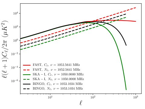
Figure 1: The noise power spectra $N_{\ell}$ (dashed line) and beam convolved angular power spectra, $C_{\ell}$ (solid line) for FAST (red), BINGO (black) and SKA-I (green) at approximately overlapped frequencies. As expected, we see that the angular power spectra have almost the same profile at large scales but deviating with increase in number of multipoles, $\ell$. Beyond $\ell=150$, angular power spectra for BINGO and SKA-I more rapidly become insignificant than noise compared to FAST angular power spectrum.

Here we vary $9$ parameters which are shown in Table 1. Therefore our Fisher matrix (Eq. (3.11)) is a $9\times 9$ matrix. To see how we can tighten up constraints with Planck satellite data, we used the best-fit $\Lambda$CDM CMB power spectra from the baseline Planck chains, that include TT + TE + EE + lensing, taken from the Planck Legacy Archive website – Cosmology section to compute the Planck covariance. We then make an entry-wise addition of the Planck Fisher matrix (the inverse of the Planck covariance (Planck Collaboration et al. 2016)) parameter respectively, to the corresponding parameter entries in the resulting Fisher matrix calculated using the formulae (3.11) for each particular Hi IM experiment. The model cosmological parameters whose values were varied by making entry-wise addition of the Planck Fisher matrix correspondingly, to BINGO, FAST and SKA-I Fisher matrices are $\Omega_{\rm b}h^{2},\ \Omega_{\rm c}h^{2},\ w_{0},\ w_{a},\ {\rm ln}(10^{10}A_{{\rm s}}),\ H_{0}$ and $n_{{\rm s}}$. The rest of Hi experiment parameters, namely, $N_{\rm eff}$ and $\Sigma m_{\nu}/94.07\ \text{eV}$, were omitted in order to only consider parameters that conform with the Planck chains dataset, Planck Collaboration et al. (2016) (believed to set strongest constraints to cosmological parameters), that we used to compute the Planck Fisher matrix under consideration.

4 Results and Discussion

In this section we present two sets of forecast results, the first one detailing various cosmological constraints comparison between FAST, BINGO and SKA-I, and the second one showing relative constraining capabilities by combining each of the three experiments with Planck. Planck covariance matrix includes TT + TE + EE + lensing, but throughout this paper, we will use a shorthand Planck to mean Planck + TT + TE + EE + lensing. Table 3 shows the $1\sigma$ errors for the marginalized parameter constraints for each of these experiments. In our simulations, for all the three experiments, we fix the frequency bandwidth to be $10$ MHz, unless stated otherwise. More specifically, the frequency (or equivalently redshift) division is done with uniformly spacing of channels, each of width $10$ MHz or $1$ MHz, depending on the tests performed. Which means for standard tests carried with a channel width of $10$ MHz, we used $30$ redshift/frequency bins for BINGO, $40$ redshift bins for FAST and 70 redshift bins for SKA-I, while for tests carried with $1$ MHz channel width, we used $300$, $400$ and $700$ redshift bins, respectively, for BINGO, FAST and SKA-I. We have used significantly narrower channel width compared to most of the previous works, for the benefits we have motivated in the later sections. Roughly, the central value of each channel width was used in calculations, that’s the sum of the lower and upper margins divided by $2$. The central value of the bin is a good approximation for sufficiently narrower bins in that we can neglect evolution of cosmological functions/backgrounds within each redshift bin, because most of the relevant functions coupled in calculations of the angular power spectra vary slowly with redshift; instead, the evolving cosmological functions are fixed to their values at the central redshift of the bin, the choice which is however motivated by Bull et al. (2015b). Full telescope specifications we used for simulations are presented in Table 2, and the descriptions of the cosmological parameters used in forecast are given in Table 1. We use Camb_sources (Challinor & Lewis 2011) to compute the raw tomographic angular power spectra Eq. (3.1) and another code we developed to simulate forecasts of cosmological parameter constraints via Fisher matrix (Subsection 3.3). We will then compare the forecasted constraints between these different experiments.

4.1 Dark Energy Constraints

We present two separate analysis, the first one is to show how FAST, BINGO, SKA-I can comparatively constrain the dark energy equation of state (EoS) in the form of $w(a)=w_{0}+w_{a}(1-a)$ (“Chevallier-Polarski-Linder parametrization” (Chevallier & Polarski 2001; Linder 2003)) and the second one is to show how each of these experiments, FAST, BINGO, SKA-I plus Planck data can constrain the dark energy equation of state. Figure 2 shows that FAST will constrain the dark energy equation of state better than BINGO, and possibly than many other currently known single-dish Hi IM approach counterparts. But SKA-I puts more stringent constraints to the dark energy equation of state than both BINGO and FAST. The $1\sigma$ errors from $(w_{0},w_{a})$ covariance matrices for BINGO, FAST and SKA-I are respectively, $(0.9293,3.5792),(0.4083,1.5878),(0.3158,0.4622)$.

To compare the relevant improvement on $1\sigma$ errors from BINGO to FAST and SKA-I, we consider the largest error of the three experiments for a particular parameter and find out the fractions of the errors that have been reduced with respect to it. For $w_{0}$, the error is reduced by $(0.9293-0.4083)/0.9293=56.06\%$ and $(0.9293-0.3158)/0.9293=66.02\%$ for FAST and SKA-I with respect to BINGO. For $w_{a}$, it is $(3.5792-1.5878)/3.5792=55.64\%$ and $(3.5792-0.4622)/3.5792=87.09\%$ for FAST and SKA-I with respect to BINGO. Therefore we can see quite significant improvement of FAST and SKA-I for future constraints on dark energy equation of state. Although the parameters $w_{0}$ and $w_{a}$ have some degeneracy, the joint constraints with Planck can improve significantly the constraints.

The fact that FAST will do better than BINGO to constrain the dark energy equation of state remains unchanged if each of the experiment is individually combined with Planck data, as shown in Figure 3. This observation is valid and is however supported by Bigot-Sazy et al. (2016), although in their paper they have used a different set of experimental parameters. As previously observed from simulations in Figure 2, again, Figure 3 shows that SKA-I will put more stringent constraints than both FAST and BINGO when each of the experiment’s Fisher matrix is added to Planck Fisher matrix. The $1\sigma$ errors for $(w_{0},w_{a})$, BINGO + Planck, FAST + Planck and SKA-I + Planck covariance matrices are respectively, $(0.0832,0.3520),(0.0791,0.3313),(0.0678,0.2679)$, implying $(w_{0},w_{a})$ constraints improve by $(4.93\%,5.88\%)$ in error reduction for FAST + Planck relative to BINGO + Planck and an improvement of $(18.51\%,23.89\%)$ error reduction in constraining $(w_{0},w_{a})$ for SKA-I + Planck relative to BINGO + Planck, see Table 3. It is very clear that, all three experiments improve dark energy constraints tremendously when the Planck Fisher matrix is added to each of the respective experiment’s Fisher matrix.

To benchmark the performance of each single-dish experiment combined with Planck relative to Planck alone, we find that the $(w_{0},w_{a})$ $1\sigma$ errors for Planck, BINGO + Planck, FAST + Planck and SKA-I + Planck are respectively, $(0.1080,0.3845),(0.0832,0.3520),(0.0791,0.3313)$ and $(0.0678,0.2679)$. The reduction in $(w_{0},w_{a})$ $1\sigma$ errors for each experiment plus Planck, respectively, imply the $(w_{0},w_{a})$ constraints improvement of $(22.96\%,8.45\%),(26.76\%,13.84\%)$ and $(37.22\%,30.33\%)$ for BINGO + Planck, FAST + Planck and SKA-I + Planck relative to Planck alone. Table 3, Figure 11, and Figure 13 summarize how the Planck-each-single-dish experiment joint constraints improve relative to the Planck data constraints alone for all the cosmological parameters considered.

Table 3: $1\sigma$ errors for FAST, BINGO, SKA-I and Planck covariance matrices, and those obtained from covariance matrices resulting from combination of each of the FAST, BINGO and SKA-I experiment’s Fisher matrix with Planck Fisher matrix.

	FAST	BINGO	SKA-I	Planck	FAST + Planck	BINGO + Planck	SKA-I + Planck
$\Omega_{\rm b}h^{2}$	$0.0090$	$0.0168$	$0.0072$	$0.0002$	$0.0001$	$0.0001$	$0.0001$
$\Omega_{\rm c}h^{2}$	$0.0061$	$0.0133$	$0.0115$	$0.0014$	$0.0011$	$0.0012$	$0.0008$
$w_{0}$	$0.4083$	$0.9293$	$0.3158$	$0.1080$	$0.0791$	$0.0832$	$0.0678$
$w_{a}$	$1.5878$	$3.5792$	$0.4622$	$0.3845$	$0.3313$	$0.3520$	$0.2679$
${\rm ln}(10^{10}A_{{\rm s}})$	$0.1681$	$0.3217$	$0.2209$	$0.0271$	$0.0240$	$0.0259$	$0.0146$
$H_{0}$	$3.6902$	$6.5433$	$4.0082$	$1.0341$	$0.5288$	$0.6171$	$0.5282$
$N_{\rm eff}$	$1.7016$	$3.3814$	$1.2486$	$--$	$--$	$--$	$--$
$n_{{\rm s}}$	$0.0201$	$0.0727$	$0.0550$	$0.0046$	$0.0043$	$0.0045$	$0.0039$
$\Omega_{\nu}h^{2}$	$0.0044$	$0.0048$	$0.0017$	$--$	$--$	$--$	$--$

In order to investigate the optimal survey volume, we consider FAST and SKA-I, and explore the range of survey areas from $2,000\ \text{deg}^{2}$ to $25,000\ \text{deg}^{2}$. Considering $(w_{0},w_{a})$ constraints, we find the optimal survey area is around $16,000\ \text{deg}^{2}$ for FAST with $T_{\rm sys}$ corresponding to $T_{\rm rec}=25\ {\rm K}$ and $9,000\ \text{deg}^{2}$ for a $T_{\rm sys}$ corresponding to $T_{\rm rec}=35\ {\rm K}$. Results show that SKA-I can survey up to a maximum area of $25,000\ \text{deg}^{2}$. This reality can be illustrated by the figure of merit (FoM) shown in Figure 4. Figure of merit is defined as (Huterer & Turner 2001; Albrecht & Bernstein 2007)

$$\text{FoM}\propto[\sigma(w_{0})\sigma(w_{a})]^{-1}\propto 1/\sqrt{\text{det}\ C(w_{0},w_{a})}.$$ (4.1)

We vary the survey area and see which $\Omega_{\rm sur}$ can maximize the FoM. As previously stated, we choose the survey area of $10,000\ \text{deg}^{2}$ that was covered by the Sloan Digital Sky Survey (SDSS) (Alam et al. 2015). The choice has a benefit of being fairly moderate and is potentially suitable for comparative and cross-correlation studies involving SDSS-like experiments, FAST and SKA-I. In addition, it is practical to choose this survey area for FAST and SKA-I comparisons because the marginal increase of FAST FoM is quite small if $\Omega_{\rm sur}>10,000$, so we will use $\Omega_{\rm sur}=10,000$ in our forecast. BINGO (Bigot-Sazy et al. 2015) can survey an approximate area of $2,500\ \text{deg}^{2}-3,000\ \text{deg}^{2}$ as shown by Li & Ma (2017); Bigot-Sazy et al. (2016), but for this particular study, we use a survey area of $3,000\ \text{deg}^{2}$ as was suggested by Bigot-Sazy et al. (2016).

Generally speaking, higher system temperature will result in higher noise spectra, which makes the constraints worse. This is well indicated by the figure of merit ( Fig. 4), as shown by the two FAST system temperatures, $T_{\rm sys}$ of $25\ \text{K}$ and $35\ \text{K}$. Low values of $1/\sqrt{\text{det}\ C(w_{0},w_{a})}$ at high system temperature means that experimental performance decreases with an increase in system temperature. For this reason, it is likely that BINGO is mostly affected because of its high overall system temperature.

Figure 2: $w_{0}$ versus $w_{a}$, $1\sigma$ (solid line) and $2\sigma$ (dashed line) cosmological constraints for FAST (red), BINGO (black) and SKA-I (green).

Figure 3: $w_{0}$ versus $w_{a}$, $1\sigma$ (solid line) and $2\sigma$ (dashed line) cosmological constraints for Planck (blue), FAST + Planck (red), BINGO + Planck (black) and SKA-I + Planck (green).

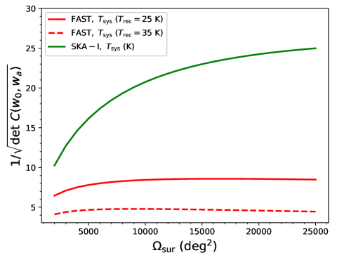
Figure 4: Figure of merit (FoM): inverse square root of the determinant of $w_{0},w_{a}$ covariance matrix, $1/\sqrt{\text{det}\ C(w_{0},w_{a})}$ versus survey area, $\Omega_{\rm sur}$ ($\text{deg}^{2}$) for FAST (red) at system with receiver temperatures, $T_{\rm rec}$, of $25\ \text{K}$ (solid line), $35\ \text{K}$ (dashed line) and for SKA-I (green) at system temperature, $T_{\rm sys}$ (K) given by Eq. (3.7).

There are several reasons why SKA-I performs better than both BINGO and FAST to constrain the dark energy equation of state. One of the reasons is the SKA-I’s wide range of frequency coverage. We split the SKA-I frequency range into lower frequency band $350\,{\rm MHz}\sim 700\,{\rm MHz}$ and high frequency band $700\,{\rm MHz}\sim 1050\,{\rm MHz}$, and compare them with the full SKA-I frequency range ($350\,{\rm MHz}\sim 1050\,{\rm MHz}$). As shown in Figure 5, the full SKA-I range of frequencies proportionately puts more stringent constraints on $w_{0}$ and $w_{a}$ than lower and upper frequency bands, and the FoM improves significantly, as shown in Figure 6. The reason is that the full frequency range of SKA-I includes the measurement of Hi power spectrum at larger range of redshift evolution, and also includes the information of cross-higher and lower frequency bands correlated signals. Therefore, it provides tighter constraints than higher and lower redshift bands.

Moreover, as we have previously accounted for BINGO, system temperature seems to be an important nuisance, which if not controlled, will severe constraints. The less stronger constraints for the SKA-I lower half of the frequency band compared to the upper band in Figure 5 (see also Figure 6) is suggestively due to high system temperatures at the corresponding frequencies. The system temperature is somewhat a function of frequency, especially parts of $T_{\rm sys}$ (3.7) that varies with it, i.e. Eqs. (3.8) and (3.9). As a result, we see that system temperature, $T_{\rm sys}$ is more dominant at low frequencies than at high frequencies, see Figure 7. This effect can as well be noted for FAST FOM at different system temperatures, Figure 4.

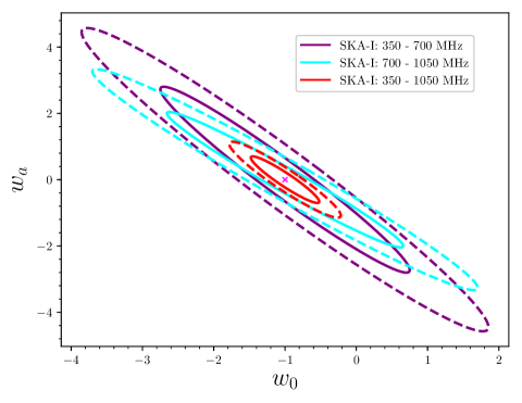
Figure 5: $w_{0}$ versus $w_{a}$, $1\sigma$ (solid line) and $2\sigma$ (dashed line) cosmological constraints for SKA-I split into lower frequency band (purple), high frequency band (cyan) and full range (red) of SKA-I frequencies.

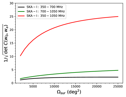
Figure 6: Figure of merit (FoM): inverse square root of the determinant of $w_{0},w_{a}$ covariance matrix, $1/\sqrt{\text{det}\ C(w_{0},w_{a})}$ versus survey area, $\Omega_{\rm sur}$ ($\text{deg}^{2}$) for various SKA-I frequency bands: lower frequency band, $350-700\ {\rm MHz}$ (black), upper frequency band, $700-1050\ {\rm MHz}$ (green), and the full SKA-I frequency range, $350-1050\ {\rm MHz}$ (red).

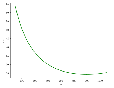
Figure 7: SKA-I variation of system temperature, $T_{\rm sys}$ against frequency, $\nu$.

The current SKA-I experimental design is to have 133 15-metre dishes and 64 13.5-metre MeerKAT dishes. We illustrate forecast with SKA-I by considering the previous number of dishes, that’s $190$ and then compare the constraint forecasts with the updated number of dishes, that’s $133$. The reason for considering the former number of dishes is to illustrate how the change in the number of dishes affects performance, and also to form a reference point for comparison with other previous literatures which considered old SKA-I (SKAI-MID) experimental specifications.

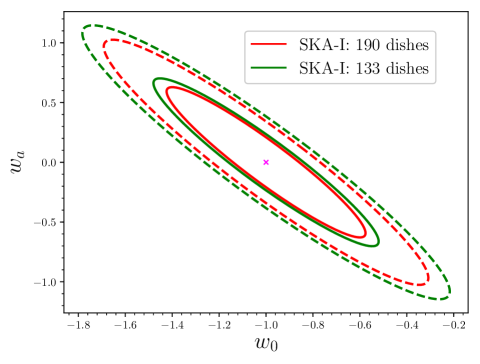
Figure 8: $1\sigma$ (solid line) and $2\sigma$ (dashed line) comparisons of SKA-I (SKAI-MID Band I) constraints on the dark energy EoS by considering early proposition of $190$ number of dishes (red), and the updated (green) $133$ number of dishes.

We see from Figure 8 that constraints do not strongly respond to the number of dishes. The most intrinsic property of large number of dishes is mapping LSS at very large angular distances/scales by integrating Hi emission efficiently over large volumes slices of the sky. One would expect that large number of dishes would significantly improve cosmological constraints, but if we compare constraints by assuming SKAI-MID $190$ and on the other hand $133$ number of single dishes, both in the autocorrelation mode, we notice not much significant difference.

The exact procedure of how to incorporate images from different frequency bands is unknown (Square Kilometre Array Cosmology Science Working Group et al. 2018), but in this forecast we assume that the SKA-I project is an integrated $190$ $15$-metre single-dishes in an autocorrelated mode for Hi intensity mapping.

4.2 Constraints of other cosmological parameters

We present the results of our forecast for the $9$ cosmological parameters in Table 1 for the single dish experiments: FAST (Nan et al. 2011; Bigot-Sazy et al. 2016), BINGO (Bigot-Sazy et al. 2015; Battye et al. 2012) and the SKA-I (Bull et al. 2015a; Santos et al. 2015). Figure 9 shows the constraints on various cosmological parameters. For the case of dark energy equation of state, we have seen that SKA-I will provide strongest constraints followed by FAST and then BINGO.

Considering all $9$ parameters, SKA-I and FAST are competitive in their abilities in constraining cosmological parameters. As shown in Figure 9, FAST provides stronger constraints on $n_{\rm s}$ because its larger dish can provide more constraints on small-scales of Hi power spectra. Interestingly, the marginalized constraints on $n_{\rm s}$ for BINGO and SKA-I do not show much significant difference. FAST will also impose stronger constraints on $\Omega_{\rm c}h^{2}$, $\text{ln}(10^{10}A_{\rm s})$ and $H_{0}$ than both BINGO and SKA-I, but slightly better constraint on $H_{0}$ than SKA-I. In comparison, SKA-I will strongly constrain $\Omega_{\nu}h^{2}$ in addition to $w_{a}$, while slightly better constraining $\Omega_{\rm b}h^{2}$ and $w_{0}$ parameters than FAST. Another observation is that SKA-I imposes slightly stronger bounds on both $N_{\rm eff}$ joint and marginalized constraints than FAST. The corresponding $\Omega_{\nu}h^{2}$, $N_{\rm eff}$ and $\Omega_{\rm b}h^{2}$ $1\sigma$ errors for SKA-I, respectively, reduces by $61.36\%$, $26.62\%$ and $20\%$ relative to FAST. Likewise, the corresponding $1\sigma$ errors for the parameters where FAST performs better than SKA-I: $n_{\rm s}$, $\Omega_{\rm c}h^{2}$, $H_{0}$, $\text{ln}(10^{10}A_{\rm s})$ respectively, are reduced by $63.45\%$, $46.96\%$, $7.93\%$, $23.9\%$ relative to the corresponding SKA-I $1\sigma$ errors. These reductions in the errors proportionately imply improvements in constraints as reflected by simulations. We depict in Figure 10 the relative constraints improvement in percentage for all parameters and for the three simulated experiments.

The prospective better performance of FAST in constraining particular parameters as we have seen, is due to its high angular resolving power. FAST has the largest dish diameter of the three telescopes which means its angular resolution is higher than that of SKA-I and BINGO by a factor of $21$ and $7.5$ respectively, making it very capable to map signals at small angular scales. So, it is likely that FAST performance will be significant at small scales. On the other hand, Figure 1 indicates FAST is noise-dominated for $\ell>100$, since its signal-to-noise ratio (SNR) is less than unity, while SKA-I does not attain SNR$<1$ until $\ell>150$. This suggests that SKA-I may better constrain cosmological parameters at some ranges of small angular scales due to its higher signal-to-noise ratio compared to FAST on those scales. Although SNR for SKA-I is greater than unity until $\ell>150$, from this point onwards, SKA-I SNR decreases exponentially, while SNR for FAST decreases gently across the same range of scales. This draws another important clue that both FAST and SKA-I can relatively perform well in constraining cosmological parameters sensitive to small angular scales. As we have previously pointed, the trade-off on whether FAST or SKA-I can perform better at small scales, may not be determined by a single factor, but a number of factors, for example, the choice of parameterization.

For the case of dark energy constraints, SKA-I stringent constraints is due to its wide frequency coverage than FAST and BINGO. BINGO is probably underprivileged due to its high system/receiver noise temperature.

Figure 11 visualizes cosmological constraints for each of these experiments combined with Planck by using Fisher matrix forecast. At this instance, constraints for all the three experiments improve significantly. As we have seen, SKA-I + Planck continues to provide better constraints than FAST + Planck and BINGO + Planck on dark energy equation of the state parameters $w_{0}$ and $w_{a}$. In contrast to the previous case involving FAST, BINGO and SKA-I experiments, SKA-I + Planck constraints on $\text{ln}(10^{10}A_{\rm s})$ and $\Omega_{\rm c}h^{2}$ relative to FAST + Planck and BINGO + Planck experiments are now very significant. Similarly, neither FAST + Planck nor SKA-I + Planck shows significant improvement in constraining $\Omega_{\rm b}h^{2}$ compared to BINGO + Planck. Therefore, SKA-I + Planck imposes strong constraints on $\Omega_{\rm c}h^{2}\ {\rm and}\ \text{ln}(10^{10}A_{\rm s})$, in addition to $w_{0},\ w_{a}$, as we have seen previously, relative to FAST + Planck and BINGO + Planck.

More specifically, SKA-I + Planck shows some significant improvement in constraining $\Omega_{\rm c}h^{2},\ {\rm and}\ \text{ln}(10^{10}A_{\rm s})$ than FAST + Planck and BINGO + Planck by respectively, $27.27\%,\ 39.17\%$ and $33.33\%,\ 43.63\%$. However, SKA-I + Planck is respectively, slightly better in constraining $n_{\rm s}$ than FAST + Planck and BINGO + Planck by $9.3\%$ and $13.33\%$.

In the like manner, FAST + Planck shows some significant improvement in constraining $\Omega_{\rm c}h^{2}$, $w_{0}$, $w_{a}$, $\text{ln}(10^{10}A_{\rm s})$, $H_{0}$ and $n_{\rm s}$ than BINGO + Planck by $8.33\%$, $4.93\%$, $5.88\%$, $7.34\%$, $14.31\%$ and $4.44\%$, respectively.

Though there is significant performance improvement in constraining most of the cosmological parameters for FAST + Planck compared to the FAST alone, for SKA-I + Planck compared to SKA-I alone and for BINGO + Planck compared to BINGO alone, there is no improvement for FAST + Planck in constraining $H_{0}$ relative to SKA-I + Planck, see Figures 11 and 12.

As we have seen from Figures 11 and 12, SKA-I + Planck, followed by FAST + Planck, are more competitive in constraining cosmological parameters than BINGO + Planck. In any case, Planck results have very significant impact to constrain cosmological parameters when combining with each of the three experiments (Fig. 13).

In addition, we have tested using the dark energy EoS and find that, for BINGO, FAST and SKA-I Hi IM experiments, the choice of frequency channel width $\Delta\nu=1$ MHz can significantly improve constraints for all the three Hi experiments than larger channel width (Fig. 14). This is because smaller band width can preserve the redshift-space-distortion effect on radial direction which makes it less “Limber canceled” than wider bandwidth (Hall et al. 2013a). This is also illustrated in figure 6 of (Xu et al. 2018).

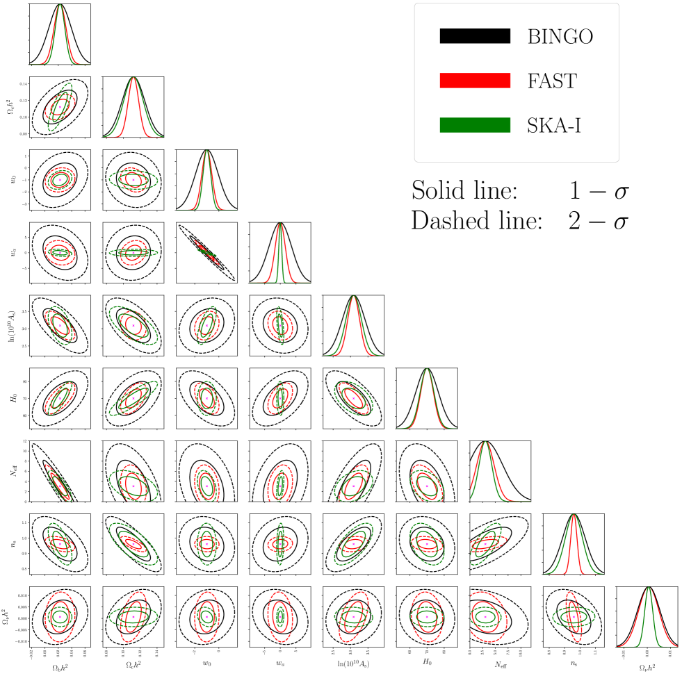
Figure 9: Forecasts of cosmological constraints with FAST, BINGO and SKA-I future observations.

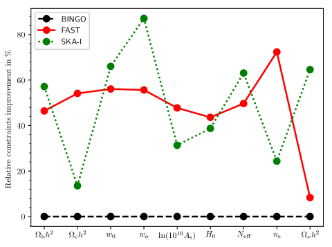
Figure 10: The relative percentage improvement for FAST and SKA-I with respect to BINGO in constraining each of the $9$ cosmological parameters.

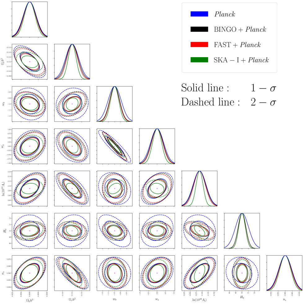
Figure 11: Forecasts of joint cosmological constraints with each of the FAST, BINGO and SKA-I experiments plus Planck data, compared with Planck data constraints alone.

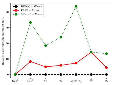
Figure 12: The relative percentage improvement for FAST + Planck and SKA-I + Planck with respect to BINGO + Planck in constraining each of the $7$ cosmological parameters we have considered.

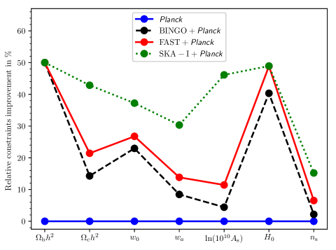
Figure 13: The relative percentage improvement for BINGO + Planck, FAST + Planck and SKA-I + Planck with respect to Planck alone in constraining each of the $7$ cosmological parameters we have considered.

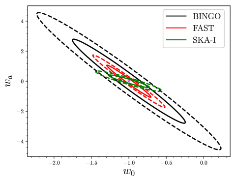
Figure 14: Forecasts of cosmological constraints with FAST, BINGO and SKA-I with a frequency channelization, $\Delta\nu=1$ MHz.

To strike a balance between limitation of foreground techniques to extract Hi signal at high angular scales and constraint prospects, as a case study, we simulate new dark energy EoS constraints by ignoring multipole moments at large angular scales, up to $\ell=9$. The comparisons between Figures 2 & 3 simulated by considering full multipole range of our interest, and Figures 15 & 16 where we apply multipole moments cut-off, by considering minimum $\ell=10$, show a conflicting scenario between foreground effects if we ignore small $\ell$’s and optimistic constraint forecast if we include them. Neglecting several values of $\ell$ corresponding to large angular scales weakens constraints, and the $1\sigma$ errors for marginalized $(w_{0},w_{a})$ constraints, changes, respectively, for BINGO, FAST and SKA-I from $(0.9293,3.5792)$, $(0.4083,1.5878)$, $(0.3158,0.4622)$ to $(1.0250,3.9449)$, $(0.4355,1.6864)$, $(0.4059,0.5735)$; and from $(0.0832,0.3520)$, $(0.0791,0.3313)$, $(0.0678,0.2679)$ to $(0.0835,0.3532)$, $(0.0795,0.3336)$, $(0.0702,0.2776)$ for BINGO + Planck, FAST + Planck, SKA-I + Planck, as summarized in Table 4.

Table 4: $1\sigma$ errors for FAST, BINGO, SKA-I covariance matrices, and those obtained from covariance matrices resulting from combination of each of the FAST, BINGO and SKA-I experiment’s Fisher matrix with Planck Fisher matrix, for minimum multipole moments, $\ell=2$ and $\ell=10$. Errors show that constraints resulting from discarding small values of $\ell$, i.e., $2\leq\ell<10$, equivalent to large angular scales are weaker than those including small $\ell$’s.

	FAST	BINGO	SKA-I	FAST + Planck	BINGO + Planck	SKA-I + Planck
$\ell\geq 2$
$w_{0}$	$0.4083$	$0.9293$	$0.3158$	$0.0791$	$0.0832$	$0.0678$
$w_{a}$	$1.5878$	$3.5792$	$0.4622$	$0.3313$	$0.3520$	$0.2679$
$\ell\geq 10$
$w_{0}$	$0.4355$	$1.0250$	$0.4059$	$0.0795$	$0.0835$	$0.0702$
$w_{a}$	$1.6864$	$3.9449$	$0.5735$	$0.3336$	$0.3532$	$0.2776$

This is a clear illustration of how large angular scales which are more dominated by the foreground contaminations, may affect the cosmological constraint forecast analyses. We will however assume that the ongoing progress in circumventing the foreground challenge and bias at large scales and other systematics at both large and small scales will be successful, and hence allowing us to consider the maximum possible range of $\ell$’s, as we have done so under this study.

The subject of foreground in general, its dominion and removal challenge on certain angular scales has been discussed in Wolz et al. (2014, 2015); Alonso et al. (2015) and the references therein; whereby Planck Collaboration et al. (2018) presents a comparative study on the performance of a number of algorithms for diffuse component separation, just to name a few.

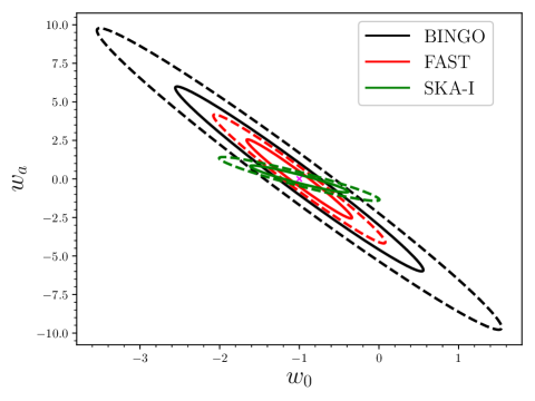
Figure 15: $w_{0}$ versus $w_{a}$, $1\sigma$ (solid line) and $2\sigma$ (dashed line) cosmological constraints for FAST (red), BINGO (black) and SKA-I (green) for minimum multipole moment, $\ell=10$.

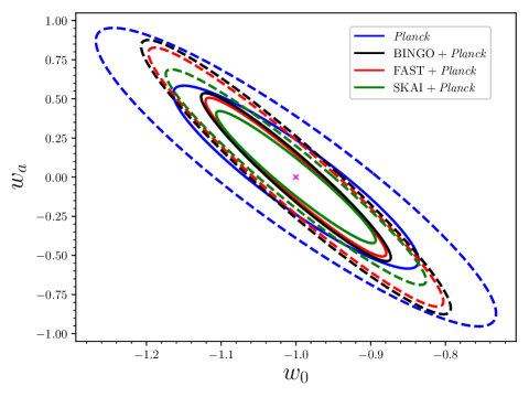
Figure 16: $w_{0}$ versus $w_{a}$, $1\sigma$ (solid line) and $2\sigma$ (dashed line) cosmological constraints for Planck (blue) FAST + Planck (red), BINGO + Planck (black) and SKA-I + Planck (green) for minimum multipole moment, $\ell=10$.

The current study is primarily focused on forecast of cosmological parameter constraints with Hi IM experiments. To this point, we postpone the in-depth discussion of the foregrounds challenge including addressing systematic limitations such as contaminations of single-dish observations by what is so called $1/f$ noise, a single instrumental systematic, due to frequency correlation, and the correlated gain fluctuations across the receiver bandpass (Harper et al. 2018) to the next issue of this series.

5 Comparison with previous forecasts of Hi IM

This forecast aims to optimize future 21cm IM experiment potentials, by providing in-depth comparative objective study focusing on FAST, BINGO and SKA-I in autocorrelation mode - a collection of independent single-dish (rather than usual interferometry) telescopes. We use much cleaner and explicit maximum likelihood and Fisher matrix tools to forecast the behavior of these three telescopes by considering a wide range of sensitive experimental analyses aspects, laying formalism that can be used to forecast varying sets of cosmological parameter constraints with a diverse range of 21cm IM experiments. We notice that there are several previous studies that have made cosmological forecasts for Hi intensity mapping experiments, but our paper has the following distinctive features:

• Extended the work by Bull et al. (2015b) to consider different cosmological parameter set. Bull et al. (2015b) considered a set of standard $\Lambda$CDM model: the Hubble parameter, $H_{0}=100h\ {\rm km\ s^{-1}\ Mpc^{-1}}$, the cosmological constant, $\Omega_{\Lambda}$, the baryons density, $\Omega_{\rm b}h^{2}$, the linear amplitude of density fluctuations, $\sigma_{8}$, the index of the power spectrum of primordial density fluctuations, $n_{\rm s}$, and the optical depth to last scattering, $\tau$. They extended the $\Lambda$CDM model with parameters $w_{0},\ w_{a},\ \Omega_{\rm K}$ and the growth index, $\gamma$. Here the cosmological constant, $\Omega_{\Lambda}$ and the curvature parameter, $\Omega_{\rm K}$ are related to the total matter density (Cold Dark Matter + baryons) by $\Omega_{\rm M}=1-\Omega_{\rm K}-\Omega_{\Lambda}$. In their forecast they used varying subsets of the considered parameters set to measure constraints. Their forecast approach included fixing fiducial values of some parameters, marginalizing over in the Planck priors Fisher matrix or over other parameters, not directly constraining some parameters by assuming their strong correlation with other parameters, such as in the case of Planck priors, where Planck measurements were combined with a particular experiment. We extended a subset of parameters considered in the aforementioned paper to form a new set, Table 1, and carried on Fisher matrix forecast, derived and treated under somewhat different approach. However, we expanded both cosmological parameters and Hi IM set of experiments compared to such papers as Battye et al. (2013) and Bigot-Sazy et al. (2015, 2016) to form a different forecast portfolio. Forecasting by considering various experimental designs and parameter sets is indispensable, since each set of cosmological parameters intertwined with a particular experimental design in principle, characterizes unique prediction results with an intention to harmoniously and comparatively contribute to address caveats and pinpoint prospects as we move towards a more precision and convergent cosmology.

• Furthermore, our forecast incorporates more recent realistic and finalized development and design information, as these telescope constructions have been undergoing major updates since the previous forecast results. These revisited experimental update set-ups, include the number of beams, dish diameter, frequency bandwidth coverage, survey area for FAST (see FAST included in the early study in Bull et al. (2015b)); and number of dishes for SKA-I, updated confirmed information about its precursor, MeerKAT and the new approach for modeling system temperatures.

  For example, previous forecasts with SKA-I considered $190$ dishes, while we make comparison, for illustration purpose using the case of dark energy EoS (see Fig. 8) in terms of SKA-I performance by considering old and updated number of dishes, we use the recently accepted and confirmed dishes for SKA-I from Square Kilometre Array Cosmology Science Working Group et al. (2018) for comparative study with BINGO and FAST.

  However, a number of previous forecasts were limited by the information made publicly available during that time. These updates are crucial, because the whole essence of forecast is to enable the Hi IM experiments to optimize their performances by considering each aspect and every single detail of their experimental designs and specifications to find out how each experiment is sensitive to various variables.

• We use a reasonably narrow and computationally effective frequency channelization with a bandwidth channel of $10\ {\rm MHz}$ each as contrasted to previous forecasts, such as Bull et al. (2015b) which considered $60\ {\rm MHz}$ for all experiments. Our consideration accounts for the role of narrower channel bandwidths, as expected for the modern radio receivers (Bull et al. 2015b) in tightening the constraints.

• We forecast for even more narrower frequency channel width of $1\ {\rm MHz}$. This choice is close to the expected channelization of the future real Hi IM surveys (Nan et al. 2011; Bigot-Sazy et al. 2016).

• In order to break degeneracies and improve precision of cosmological constraints, we include Planck 2015 CMB priors measurements that have been rigorously tested and improved, they include, CMB lensing reconstruction; TT, TE, EE Planck Cosmic Microwave Background (CMB) (Bennett et al. (2013)) power spectra; where TT represents temperature power spectrum, TE is temperature-polarization cross-spectrum, and EE is polarization power spectrum; and high $\ell$ CMB measurements. This was not objectively considered by even the forecasts such as those which tried to include as many experiments as possible.

• We have provided more extensive quantification of cosmological constraints forecast in regard to these representative telescopes of our choice focusing on Hi IM surveys. Other related works such as Villaescusa-Navarro et al. (2017) have studied the BAOs measurements through a single-dish Hi IM observations in the post-reionization epoch in the light of SKAI-MID. Shaw et al. (2014, 2015) have alternatively addressed forecast of cosmological constraints, Hi power spectrum estimation and measurement analyses of wide-field transient telescopes such as CHIME by an approach of what they call m-mode formalism. Furthermore, Pourtsidou et al. (2017) forecasted Hi evolution with redshift and a select subset of model-independent cosmological parameters focusing on the performance of the SKA and its precursor MeerKAT Hi IM surveys (Pourtsidou 2017), proposing their cross-correlation with optical galaxy surveys. Under different setting, constraints on the dark energy parameters by cross-correlating/combining SKA-like Hi IM and LSST-like surveys have been performed by Pourtsidou et al. (2015).

  The essence of cross-correlating Hi IM or 21cm maps in general with galaxy redshift surveys, is that contaminants, such as foregrounds, various noises and systematics between the maps from two types of surveys are largely expected to be uncorrelated in frequency; this is in contrast to Hi signal which is correlated in respective frequency bands. As a result, cross-correlation will statistically boost the abundance and the amplitude of Hi signal, but also statistically cancel out relevant foregrounds and systematics, thus increasing Hi signal detection, and consequently improve constraints on the estimated values of the cosmological and astrophysical parameters. Constraints of $\Omega_{\rm HI}b_{\rm HI}r$ have direct link to the future IM surveys capabilities and the prospect science outputs, and these surveys heavily depend on the qualitative and quantitative measurements (such as shape and amplitude) of Hi signal. Cross-correlation will thus aggregate more Hi signal information than any individual experiments, yielding robust and precise cosmological measurements (Pourtsidou 2017). Pourtsidou et al. (2017), for example, has reported improvement to about a factor $\sim 3$ by considering Stage IV spectroscopic galaxy survey (similar to EUCLID) and MeerKAT with an overlap area of $500\ {\rm deg}^{2}$ in constraining the amplitude of the quantity $\Omega_{\rm HI}b_{\rm HI}r$, where $r$ is a correlation coefficient that accounts for possible stochasticity in the galaxy and Hi tracers (Pourtsidou 2017). Similarly, with an overlap area of $4000\ {\rm deg}^{2}$, cross-correlation between MeerKAT and Stage III photometric optical galaxy survey measured/constrained $\Omega_{\rm HI}b_{\rm HI}r$ at $\sim 5$ percent level across a wide range of redshifts compared to the autocorrelated MeerKAT constraints. According to them, such improvements were better than autocorrelation results they could achieve. The fact that the cross-correlated power spectrum will be less sensitive to contaminations, can be used to identify systematics in 21cm maps (Wolz et al. 2016; Pourtsidou et al. 2017; Carucci et al. 2017). Cross-correlation could be less susceptible to systematic contaminants (Pourtsidou et al. 2015), hence foregrounds and systematics are expected to be highly suppressed, respectively, making their removal and control much easier.

  Furlanetto & Lidz (2007) has laid down several advantages of cross-correlation, two of them are: firstly, the signal-to-noise ratio resulting from cross-correlating 21cm experiments and galaxy redshift surveys exceeds that of the individual 21cm power spectrum by a factor of few, further asserting that, this may allow probing of smaller spatial scales and possibly more efficient detection of inhomogeneous reionization. Secondly, the approach highly reduces the required level of foreground cleaning for the 21cm signal/maps. Hi IM and galaxy redshift survey cross-correlation approach to suppress foregrounds and systematics has also been motivated, explored and echoed using simulations by a number of other authors, some of them include Wolz et al. (2016); Carucci et al. (2017); Cunnington et al. (2019). This observation is also supported by Pen et al. (2009); Chang et al. (2010); Switzer et al. (2013); Masui et al. (2013b); Anderson et al. (2017) who achieved the detection of Hi by cross-correlating the Hi IM and optical galaxy redshift surveys. Synergized cross-correlation between these two types of surveys has mutual benefits, that make them complement each other in alleviating survey-specific systematic effects and boost Hi signal detection.

  Other forecasts include CMB bounds on $f_{\rm NL}$ by combining information from SKA Phase I and Euclid/LSST-like photometric galaxy surveys using multi-tracer, contrasting with respective single-tracer measurements (Fonseca et al. 2015); and an extension of this approach for Hi IM with MeerKAT and photometric galaxy survey to constrain $f_{\rm NL}$ and a number of other parameters (Fonseca et al. 2017b).

• Although combination of different subsets of cosmological parameters and experimental designs largely characterize the future telescope performances, this study has singled out those features intrinsic to the particular experiment and are likely to determine their performance reliability, consistency and stability in benchmarking with other similar surveys.

In this paper, we have, therefore, intentionally addressed forecasts of cosmological constraints for the three Hi IM experiments under consideration, while including issues previously not given significant attention, updating the forecasts to suit the upgrades undergone by the considered telescopes and individually and simultaneously comparatively asses the three telescope performances while laying down a basis for any other cosmological constraints forecast with Hi IM experiments, as we prepare for real survey take-off with these next generation instruments. A great deal of useful information we aggregate through our researches play a complementary role in building a scientific body of knowledge that can be maximally deployed to continually study the Universe.

6 Conclusion

We have conducted forecasts for cosmological constraints (Figs. 2, 3, 9, 11) for a set of $9$ cosmological parameters (Table 1) and compared performance for three different proposed future survey projects, FAST, BINGO and SKA-I. Our results, with a prescribed choice of experimental parameter set (Table 2) show that FAST experiment will have better performance compared to BINGO, particularly, in constraining dark energy equation of state. In overall, SKA-I will put more stringent constraints for the dark energy equation of state than FAST and BINGO. We notice that, there is a trade-off between SKA-I and FAST in constraining cosmological parameters, with each experiment being more superior in constraining a particular set of parameters.

We point out that narrower frequency bandwidth such as $1\ \text{MHz}$ (see Fig. 14) greatly improves constraints because the redshift-space-distortion effect suffers less cancellation if frequency band becomes narrower (Hall et al. 2013a; Xu et al. 2018). But this requires more computer resources in terms of memory (RAM) for intermediate storage and speed for reasonable computational time. This challenge can however be addressed by advancing computing resources and modeling strategy. We postulate that, high frequency resolution needs one to take into account correlated noise residues at $i$-th and $j$-th frequency bins which would become noticeable due to many frequency channels being correlated, otherwise noise residues would be significant to be ignored and in some way impact the results. However, real instrumentation will use much narrower frequency bandwidth which would facilitate radio frequency interference excision (Nan et al. 2011).

We conclude that for a single-dish approach, BINGO, FAST and SKA-I will progressively provide stronger constraints on dark energy equation of the state and other cosmological parameters. The constraints can be further improved by combining with CMB experiment such as Planck data.

We performed Hi IM Fisher matrix forecast for BINGO, FAST and SKA-I radio telescopes, and extended similar comparative analysis for each of the three experiments’ data, combined with Planck chains, (Planck Collaboration et al. 2014) which have considerably tighten the cosmological constraints. This substantial and objective comparative analysis of simulated forecast results provides a benchmark on the relative expected performances of BINGO, FAST and SKA-I experiments under relatively similar settings in constraining an extended number of cosmological parameters in Table 1. FAST, BINGO, SKA-I and many other telescopes are suitable for Hi IM, and some will even do a wide range of sciences (Nan et al. 2011) than others. Our aim is not to show the superiority or inferiority of these experiments against each other, but to illustrate a global picture on their relative prospects. Our results can however, signal for adjustment, revision of specification configurations, or for further calibration where there is a possibility in order to rectify and optimize capabilities so that these telescopes can fulfil their promise.

This paper sets an important mark for our series of works to study IM surveys with HI. Future proceedings will feature applicability and quantification of this novel but a promising approach by developing IM pipeline to simulate sky maps for various sky emissions, addressing and testing different foreground cleaning methods, investigating and quantifying various calibration issues. These realistic issues include bandpass calibration, systematics and other uncertainty measurements, studying and developing solid knowledge of polarization purity, and measuring BAO wiggles from Hi power spectrum and consequently developing more stringent constraints on dark energy, dark matter and other cosmological parameters.

7 Acknowledgements

E.Y. acknowledges the DAAD (German Academic Exchange Service) scholarship and the financial support from The African Institute for Mathematical Sciences, University of KwaZulu-Natal, and The Dar Es Salaam University College of Education, Tanzania. Y.C.L. and Y.Z.M. acknowledge support from the National Research Foundation of South Africa (Grant No. 105925 and 110984).

References

- Alam et al. (2015) Alam, S., Albareti, F. D., Allende Prieto, C., et al. 2015, The Astrophysical Journal Supplement Series, 219, 12
- Alam et al. (2017) Alam, S., Ata, M., Bailey, S., et al. 2017, Monthly Notices of the Royal Astronomical Society, 470, 2617
- Albrecht & Bernstein (2007) Albrecht, A., & Bernstein, G. 2007, Physical Review D, 75, 103003
- Alonso et al. (2015) Alonso, D., Bull, P., Ferreira, P. G., & Santos, M. G. 2015, Monthly Notices of the Royal Astronomical Society, 447, 400
- Anderson et al. (2017) Anderson, C. J., Luciw, N. J., Li, Y.-C., et al. 2017, arXiv:1710.00424
- Anderson et al. (2012) Anderson, L., Aubourg, E., Bailey, S., et al. 2012, Monthly Notices of the Royal Astronomical Society, 427, 3435
- Bandura et al. (2014) Bandura, K., Addison, G. E., Amiri, M., et al. 2014, in Proceedings of SPIE, Vol. 9145, Ground-based and Airborne Telescopes V, 914522
- Battye et al. (2013) Battye, R. A., Browne, I. W. A., Dickinson, C., et al. 2013, Monthly Notices of the Royal Astronomical Society, 434, 1239
- Battye et al. (2012) Battye, R. A., Brown, M. L., Browne, I. W. A., et al. 2012, arXiv:1209.1041
- Battye et al. (2016) Battye, R., Browne, I., Chen, T., et al. 2016, arXiv:1610.06826
- Bennett et al. (2013) Bennett, C. L., Larson, D., Weiland, J. L., et al. 2013, The Astrophysical Journal Supplement Series, 208, 20
- Beutler et al. (2011) Beutler, F., Blake, C., Colless, M., et al. 2011, Monthly Notices of the Royal Astronomical Society, 416, 3017
- Bigot-Sazy et al. (2015) Bigot-Sazy, M.-A., Dickinson, C., Battye, R. A., et al. 2015, Monthly Notices of the Royal Astronomical Society, 454, 3240
- Bigot-Sazy et al. (2016) Bigot-Sazy, M.-A., Ma, Y.-Z., Battye, R. A., et al. 2016, in Astronomical Society of the Pacific Conference Series, Vol. 502, Frontiers in Radio Astronomy and FAST Early Sciences Symposium 2015, ed. L. Qain & D. Li, 41
- Blake et al. (2008) Blake, C., Brough, S., Couch, W., et al. 2008, Astronomy and Geophysics, 49, 5.19
- Blake et al. (2011) Blake, C., Kazin, E. A., Beutler, F., et al. 2011, Monthly Notices of the Royal Astronomical Society, 418, 1707
- Braun et al. (2015) Braun, R., Bourke, T., Green, J. A., Keane, E., & Wagg, J. 2015, Advancing Astrophysics with the Square Kilometre Array (AASKA14), 174
- Bull (2016) Bull, P. 2016, The Astrophysical Journal, 817, 26
- Bull et al. (2015a) Bull, P., Camera, S., Raccanelli, A., et al. 2015a, Advancing Astrophysics with the Square Kilometre Array (AASKA14), 24
- Bull et al. (2015b) Bull, P., Ferreira, P. G., Patel, P., & Santos, M. G. 2015b, The Astrophysical Journal, 803, 21
- Camacho et al. (2018) Camacho, H., Kokron, N., Andrade-Oliveira, F., et al. 2018, arXiv:1807.10163
- Camera et al. (2018) Camera, S., Fonseca, J., Maartens, R., & Santos, M. G. 2018, Monthly Notices of the Royal Astronomical Society, 481, 1251
- Camera et al. (2015) Camera, S., Santos, M. G., & Maartens, R. 2015, Monthly Notices of the Royal Astronomical Society, 448, 1035
- Carucci et al. (2017) Carucci, I. P., Villaescusa-Navarro, F., & Viel, M. 2017, Journal of Cosmology and Astro-Particle Physics, 2017, 001
- Challinor & Lewis (2011) Challinor, A., & Lewis, A. 2011, Physical Review D, 84, 043516
- Chang et al. (2010) Chang, T.-C., Pen, U.-L., Bandura, K., & Peterson, J. B. 2010, Nature, 466, 463
- Chang et al. (2008) Chang, T.-C., Pen, U.-L., Peterson, J. B., & McDonald, P. 2008, Physical Review Letters, 100, 091303
- Chen (2012) Chen, X. 2012, in International Journal of Modern Physics Conference Series, Vol. 12, International Journal of Modern Physics Conference Series, 256
- Chevallier & Polarski (2001) Chevallier, M., & Polarski, D. 2001, International Journal of Modern Physics D, 10, 213
- Colless et al. (2001) Colless, M., Dalton, G., Maddox, S., et al. 2001, Monthly Notices of the Royal Astronomical Society, 328, 1039
- Cunnington et al. (2019) Cunnington, S., Wolz, L., Pourtsidou, A., & Bacon, D. 2019, arXiv e-prints, arXiv:1904.01479
- Dark Energy Survey Collaboration et al. (2016) Dark Energy Survey Collaboration, Abbott, T., Abdalla, F. B., et al. 2016, Monthly Notices of the Royal Astronomical Society, 460, 1270
- Davis et al. (2001) Davis, M., Newman, J. A., Faber, S. M., & Phillips, A. C. 2001, in Deep Fields, ed. S. Cristiani, A. Renzini, & R. E. Williams, 241
- DESI Collaboration et al. (2016) DESI Collaboration, Aghamousa, A., Aguilar, J., et al. 2016, arXiv:1611.00036
- Di Dio et al. (2014) Di Dio, E., Montanari, F., Durrer, R., & Lesgourgues, J. 2014, Journal of Cosmology and Astro-Particle Physics, 2014, 042
- Dickinson (2014) Dickinson, C. 2014, arXiv:1405.7936
- Dodelson (2003) Dodelson, S. 2003, Modern cosmology
- Fonseca et al. (2015) Fonseca, J., Camera, S., Santos, M. G., & Maartens, R. 2015, Astrophysical Journal Letters, 812, L22
- Fonseca et al. (2017a) Fonseca, J., Maartens, R., & Santos, M. G. 2017a, Monthly Notices of the Royal Astronomical Society, 466, 2780
- Fonseca et al. (2017b) Fonseca, J., Maartens, R., & Santos, M. G. 2017b, Monthly Notices of the Royal Astronomical Society, 466, 2780
- Furlanetto & Lidz (2007) Furlanetto, S. R., & Lidz, A. 2007, The Astrophysical Journal, 660, 1030
- Green et al. (2012) Green, J., Schechter, P., Baltay, C., et al. 2012, arXiv:1208.4012
- Hall et al. (2013a) Hall, A., Bonvin, C., & Challinor, A. 2013a, Physical Review D, 87, 064026
- Hall et al. (2013b) Hall, A., Bonvin, C., & Challinor, A. 2013b, Physical Review D, 87, 064026
- Harper et al. (2018) Harper, S. E., Dickinson, C., Battye, R. A., et al. 2018, Monthly Notices of the Royal Astronomical Society, 478, 2416
- Haynes (2008) Haynes, M. P. 2008, in Astronomical Society of the Pacific Conference Series, Vol. 395, Frontiers of Astrophysics: A Celebration of NRAO’s 50th Anniversary, ed. A. H. Bridle, J. J. Condon, & G. C. Hunt, 125
- Huterer & Turner (2001) Huterer, D., & Turner, M. S. 2001, Physical Review D, 64, 123527
- Ivezic et al. (2008) Ivezic, Z., Tyson, J. A., Abel, B., et al. 2008, arXiv:0805.2366
- Jones et al. (2009) Jones, D. H., Read, M. A., Saunders, W., et al. 2009, Monthly Notices of the Royal Astronomical Society, 399, 683
- Kazin et al. (2014) Kazin, E. A., Koda, J., Blake, C., et al. 2014, Monthly Notices of the Royal Astronomical Society, 441, 3524
- Kovetz et al. (2017) Kovetz, E. D., Viero, M. P., Lidz, A., et al. 2017, arXiv:1709.09066
- Laureijs et al. (2011) Laureijs, R., Amiaux, J., Arduini, S., et al. 2011, arXiv:1110.3193
- Levi et al. (2013) Levi, M., Bebek, C., Beers, T., et al. 2013, arXiv:1308.0847
- Lewis & Challinor (2006) Lewis, A., & Challinor, A. 2006, Physics Reports, 429, 1
- Lewis & Challinor (2007) Lewis, A., & Challinor, A. 2007, Physical Review D, 76, 083005
- Li & Ma (2017) Li, Y.-C., & Ma, Y.-Z. 2017, Physical Review D, 96, 063525
- Linder (2003) Linder, E. V. 2003, Phys. Rev. Lett., 90, 091301
- Loeb & Wyithe (2008) Loeb, A., & Wyithe, J. S. B. 2008, Physical Review Letters, 100, 161301
- LSST Science Collaboration et al. (2009) LSST Science Collaboration, Abell, P. A., Allison, J., et al. 2009, arXiv:0912.0201
- Masui et al. (2013a) Masui, K. W., Switzer, E. R., Banavar, N., et al. 2013a, Astrophysical Journal Letters, 763, L20
- Masui et al. (2013b) Masui, K. W., Switzer, E. R., Banavar, N., et al. 2013b, Astrophysical Journal Letters, 763, L20
- Nan et al. (2011) Nan, R., Li, D., Jin, C., et al. 2011, International Journal of Modern Physics D, 20, 989
- Newburgh et al. (2016) Newburgh, L. B., Bandura, K., Bucher, M. A., et al. 2016, in Proceedings of SPIE, Vol. 9906, Ground-based and Airborne Telescopes VI, 99065X
- Pen et al. (2009) Pen, U.-L., Staveley-Smith, L., Peterson, J. B., & Chang, T.-C. 2009, Monthly Notices of the Royal Astronomical Society, 394, L6
- Planck Collaboration et al. (2014) Planck Collaboration, Ade, P. A. R., Aghanim, N., et al. 2014, Astronomy and Astrophysics, 571, A16
- Planck Collaboration et al. (2016) Planck Collaboration, Ade, P. A. R., Aghanim, N., et al. 2016, Astronomy and Astrophysics, 594, A13
- Planck Collaboration et al. (2018) Planck Collaboration, Aghanim, N., Akrami, Y., et al. 2018, arXiv:1807.06209
- Pourtsidou (2017) Pourtsidou, A. 2017, arXiv:1709.07316
- Pourtsidou et al. (2015) Pourtsidou, A., Bacon, D., & Crittenden, R. 2015, arXiv:1506.02615
- Pourtsidou et al. (2017) Pourtsidou, A., Bacon, D., & Crittenden, R. 2017, Monthly Notices of the Royal Astronomical Society, 470, 4251
- Pritchard & Loeb (2012) Pritchard, J. R., & Loeb, A. 2012, Reports on Progress in Physics, 75, 086901
- Ross et al. (2012) Ross, N. P., Myers, A. D., Sheldon, E. S., et al. 2012, The Astrophysical Journal Supplement Series, 199, 3
- Santos et al. (2017) Santos, M. G., Cluver, M., Hilton, M., et al. 2017, arXiv:1709.06099
- Santos et al. (2015) Santos, M., Bull, P., Alonso, D., et al. 2015, Advancing Astrophysics with the Square Kilometre Array (AASKA14), 19
- Schneider et al. (1992) Schneider, P., Ehlers, J., & Falco, E. E. 1992, Gravitational Lenses, 112
- Shaw & Lewis (2008) Shaw, J. R., & Lewis, A. 2008, Physical Review D, 78, 103512
- Shaw et al. (2014) Shaw, J. R., Sigurdson, K., Pen, U.-L., Stebbins, A., & Sitwell, M. 2014, The Astrophysical Journal, 781, 57
- Shaw et al. (2015) Shaw, J. R., Sigurdson, K., Sitwell, M., Stebbins, A., & Pen, U.-L. 2015, Physical Review D, 91, 083514
- Smoot & Debono (2017) Smoot, G. F., & Debono, I. 2017, Astronomy and Astrophysics, 597, A136
- Square Kilometre Array Cosmology Science Working Group et al. (2018) Square Kilometre Array Cosmology Science Working Group, Bacon, D. J., Battye, R. A., et al. 2018, arXiv:1811.02743
- Switzer et al. (2013) Switzer, E. R., Masui, K. W., Bandura, K., et al. 2013, Monthly Notices of the Royal Astronomical Society, 434, L46
- Tansella et al. (2018) Tansella, V., Bonvin, C., Durrer, R., Ghosh, B., & Sellentin, E. 2018, Journal of Cosmology and Astro-Particle Physics, 2018, 019
- The LSST Dark Energy Science Collaboration et al. (2018) The LSST Dark Energy Science Collaboration, Mandelbaum, R., Eifler, T., et al. 2018, arXiv:1809.01669
- Troxel et al. (2017) Troxel, M. A., MacCrann, N., Zuntz, J., et al. 2017, arXiv:1708.01538
- Villaescusa-Navarro et al. (2017) Villaescusa-Navarro, F., Alonso, D., & Viel, M. 2017, Monthly Notices of the Royal Astronomical Society, 466, 2736
- Wolz et al. (2014) Wolz, L., Abdalla, F. B., Blake, C., et al. 2014, Monthly Notices of the Royal Astronomical Society, 441, 3271
- Wolz et al. (2016) Wolz, L., Tonini, C., Blake, C., & Wyithe, J. S. B. 2016, Monthly Notices of the Royal Astronomical Society, 458, 3399
- Wolz et al. (2015) Wolz, L., Blake, C., Abdalla, F. B., et al. 2015, arXiv:1510.05453
- Xu et al. (2018) Xu, X., Ma, Y.-Z., & Weltman, A. 2018, Physical Review D, 97, 083504
- Yoo (2009) Yoo, J. 2009, Physical Review D, 79, 023517
- Yoo (2010) Yoo, J. 2010, Physical Review D, 82, 083508
- Yoo et al. (2009) Yoo, J., Fitzpatrick, A. L., & Zaldarriaga, M. 2009, Physical Review D, 80, 083514
- York et al. (2000) York, D. G., Adelman, J., Anderson, Jr., J. E., et al. 2000, The Astronomical Journal, 120, 1579
- Zwaan et al. (2004) Zwaan, M. A., Meyer, M. J., Webster, R. L., et al. 2004, Monthly Notices of the Royal Astronomical Society, 350, 1210