UKRmol+: a suite for modelling of electronic processes in molecules interacting with electrons, positrons and photons using the R-matrix method

Abstract

UKRmol+ is a new implementation of the UK R-matrix electron-molecule scattering code. Key features of the implementation are the use of quantum chemistry codes such as Molpro to provide target molecular orbitals; the optional use of mixed Gaussian – B-spline basis functions to represent the continuum and improved configuration and Hamiltonian generation. The code is described, and examples covering electron collisions from a range of targets, positron collisions and photionisation are presented. The codes are freely available as a tarball from Zenodo.

PROGRAM SUMMARY

Program Title: UKRmol+
Licensing provisions: GNU GPLv3
Programming language: Fortran 95 with use of some Fortran 2003 features
Program repository available at: https://gitlab.com/UK-AMOR/UKRmol
Computers on which the program has been tested: Cray XC30 ARCHER, Lenovo SD530 node (UCL’s Myriad), TACC Stampede2, Intel pcs.
Number of processors used: Min: 1, Max tested: program dependent, up to 100 cores for the parallel ones
Number of lines in program: 158178 in UKRmol-in (including GBTOlib) and 79760 in UKRmol-out
Distribution format: Tarball available from Zenodo (https://zenodo.org/)
External routines/libraries: LAPACK, BLAS; optionally MPI, ScaLAPACK, Arpack, SLEPc

Nature of problem: The computational study of electron and positron scattering from a molecule requires the determination of multicentric time-independent wavefunctions describing the target+projectile system. These wavefunctions can also be used to calculate photoionization cross sections (in this case the free particle is the ionized electron) or provide input for time-dependent calculations of laser-induced ultrafast processes.

Solution method: We use the R-matrix method [1], that partitions space into an ‘inner’ and an ‘outer’ region. In the inner region (within a few tens of a₀ of the nuclei at most) exchange and correlation are taken into account. In the outer region, where the free particle is distinguishable from the target electrons, a single-centre multipole potential describes its interaction with the molecule. The key computational step is the building and diagonalization of the target + free particle Hamiltonian in the inner region, making use of integrals generated using the GBTOlib library. The eigenpairs obtained are then used as input to outer region suite programs to determine scattering quantities (K-matrices, etc.) or transition dipole moments and, from them, photoionization cross sections. The suite also generates input data for the R-matrix with time (RMT) suite [2].

Additional comments: CMake scripts for the configuration, compilation, testing and installation of the suite are provided. This article describes the release version UKRmol-in 3.0, that uses GBTOlib 2.0, and UKRmol-out 3.0.

1 Introduction

The R-matrix method is a form of embedding method which involves the division of space into a (spherical) inner region and an outer region. It is widely used for theoretical studies in atomic, molecular and optical physics [1, 2], nuclear physics [3] and recently ultra-cold chemistry [4]. A feature of the R-matrix method for scattering applications is that the inner region problem is independent of the scattering energy. This means that solution of the inner region only needs to be performed once and that the energy dependence of the problem is confined to the physically simpler outer region. This facilitates, for example, the use of fine energy meshes which can be important for finding and characterising resonances (metastable states embedded in the continuum).

The UK molecular R-matrix codes are an implementation of the R-matrix method originally designed for treating electron-molecule collisions. They have been subsequently generalised to treat other processes such photoionisation, positron molecule collisions [5] and studies of diffuse bound states. Theses codes have been developed over a number of years [6, 7, 8].

The present paper reports the release of a new version of the codes, known as UKRmol+. UKRmol+ represents a major improvement in functionality, algorithms and parallelisation compared to the previous version known as UKRmol. In particular, UKRmol+ allows the optional use of B-spline basis functions to represent the continuum which facilitates calculations with higher kinetic energies of the free electron and the use of greatly enlarged inner regions allowing both large targets and targets with more diffuse electronic states to be studied. Previous versions of the UKRmol codes have incorporated a (limited) quantum chemistry capability to provide target orbitals. In a change from this, UKRmol+ utilizes external electronic structure codes (e.g. Molpro [9]) to provide molecular orbitals allowing considerably more flexibility in the representation of the molecular targets. Algorithmic improvements include use of the new GBTOlib library [10] for computing integrals, generating configurations and constructing the Hamiltonian matrix among others. These new modules are designed to take advantage of MPI, where available, an option not available in the older code. In addition, UKRmol+ contains an option to compute photoionisation dipoles and cross sections [11, 12] plus these dipoles can also be used as the input for the RMT (R-matrix with time) code [13] which can treat molecules in intense, ultrashort, arbitrarily-polarized laser pulses. A number of other improvements in functionality are discussed below.

We note that some of the works containing results that are referenced throughout the papers actually used the UKRmol suite. UKRmol+ should be able to reproduce virtually all the old results (some functionality has yet to be implemented in the new suite); this has indeed been tested for a number of targets.

This paper is structured as follows. Section 2 introduces the molecular R-matrix theory: a succinct derivation in Section 2.1 will help those readers interested in a deeper understanding of the background of the method; those interested in how the quantities generated by the suite combine to solve the scattering/photoionization problem and the R-matrix scattering models used in practice can safely avoid this derivation. Section 3 details the input data required and the capabilities of each program in the suite. Sections 4, 5 and 6 describe how the programs in suite are combined to study electron/positron scattering, photoionization and to produce input for the RMT suite respectively. The test suite is described in Section 7 followed by Section 8 containing several examples of practical applications which illustrate the current capabilities of the suite.

2 Overview of the R-matrix approach

In the R-matrix method space is divided by a so-called R-matrix sphere of radius $a$. This radius needs to be set large enough to ensure that the wavefunction representing the target can be assumed to have zero amplitude on the boundary (in fact, all target orbitals used should have approximately zero amplitude on the boundary). As explained below, this division allows us to solve the Schrödinger equation separately in these two parts and join the solution on the R-matrix sphere. A full exposition of the R-matrix theory can be found in the monographs [14, 15]. In this Section, we start by deriving the fundamental equations of the R-matrix method. Readers interested only in the main equations implemented in the suite can skip this derivation and start with Section 2.2.

2.1 Derivation of the approach

We wish to find the solution of the multi-electron Schrödinger equation in the whole space for a problem where one of the (total) N+1 electrons (or a positron) can be found outside of the R-matrix sphere ($r\geq a$). Here correlation and exchange with the inner region can be neglected and the outer-region particle can be regarded as moving in a generally non-spherical static potential of the molecule (Appendix A.2 in [13] details the form of this potential). The total wavefunction in the outer region can therefore be written using the channel expansion

$$|\Psi_{out}(E)\rangle=\sum_{p}^{n}\frac{F_{pp^{\prime}}(r_{N+1})}{r_{N+1}}\overline{\Phi}_{p}^{\Gamma}({\mathbf{X}}_{N};{\hat{\mathbf{r}}}_{N+1}\sigma_{N+1}),$$ (1)

where $\overline{\Phi}_{p}^{\Gamma}({\mathbf{X}}_{N};{\hat{\mathbf{r}}}_{N+1}\sigma_{N+1})$ is the channel wavefunction given by a product of the wavefunction representing a target electronic state and the angular (spherical harmonic) part of the wavefunction of the outer region electron and $n$ is the total number of channels. $\mathbf{X}_{N}$ stands for all spin-space coordinates of the N electrons confined to the inner region and $\hat{\mathbf{r}}_{N+1}\sigma_{N+1}$ are the angular and spin coordinates of the (N+1)th particle (electron/positron) and $r_{N+1}$ is its radial coordinate. From now on we drop the index of the (N+1)th particle when referring to its coordinates. The functions $F_{pp^{\prime}}(r)$ are the reduced radial wavefunctions of the outer region particle and $p^{\prime}$ labels the linearly independent solutions of the single-particle Schrödinger equation. As the analytic form of these functions is well known in the asymptotic region [16, 11], we can match outer region solutions with the ones from the inner region, $|\Psi_{in}(E)\rangle$:

$$H_{N+1}|\Psi_{in}(E)\rangle = E|\Psi_{in}(E)\rangle,$$ (2)

$$\langle\overline{\Phi}_{p}^{\Gamma}\mbox{\small$\frac{1}{r}$}|\Psi_{in}(E)\rangle\big{|}_{r=a} = \langle\overline{\Phi}_{p}^{\Gamma}\mbox{\small$\frac{1}{r}$}|\Psi_{out}(E)\rangle\big{|}_{r=a},p=1,\dots,n,$$ (3)

$$\frac{d}{dr}\langle\overline{\Phi}_{p}^{\Gamma}\mbox{\small$\frac{1}{r}$}|\Psi_{in}(E)\rangle\bigg{|}_{r=a} = \frac{d}{dr}\langle\overline{\Phi}_{p}^{\Gamma}\mbox{\small$\frac{1}{r}$}|\Psi_{out}(E)\rangle\bigg{|}_{r=a},p=1,\dots,n.$$ (4)

Here $E$ is the total energy and $H_{N+1}$ is the non-relativistic molecular Hamiltonian in the fixed-nuclei approximation

$$H_{N+1} = \sum_{i=1}^{N+1}\left(-\frac{1}{2}\nabla_{i}^{2}+\sum_{i>j}^{N+1}\frac{1}{|\mathbf{r}_{i}-\mathbf{r}_{j}|}-\sum_{k=1}^{Nuclei}\frac{Z_{k}}{|\mathbf{r}_{i}-\mathbf{R}_{k}|}\right).$$ (5)

where $Z_{k}$ is the charge and $\mathbf{R}_{k}$ is the position of the nucleus. Note that equations (3-4) are equivalent to:

$$F_{pp^{\prime},in}(a) = F_{pp^{\prime},out}(a),$$ (6)

$$F_{pp^{\prime},in}^{{}^{\prime}}(a) = F_{pp^{\prime},out}^{{}^{\prime}}(a).$$ (7)

The R-matrix method is an equivalent formulation of this boundary value problem which uses the Bloch operator, $L$, to embed the second (derivative) boundary condition into the solution of the Schrödinger equation (2)

$$(H_{N+1}+L)|\Psi_{in}(E)\rangle = E|\Psi_{in}(E)\rangle+L|\Psi_{out}(E)\rangle,$$ (8)

$$\langle\overline{\Phi}_{p}^{\Gamma}\mbox{\small$\frac{1}{r}$}|\Psi_{in}(E)\rangle\big{|}_{r=a} = \langle\overline{\Phi}_{p}^{\Gamma}\mbox{\small$\frac{1}{r}$}|\Psi_{out}(E)\rangle\big{|}_{r=a},p=1,\dots,n,$$ (9)

$$L = \sum_{i=1}^{N+1}\frac{1}{2}\delta(r_{i}-a)\frac{d}{dr_{i}}.$$ (10)

The Bloch operator ensures that the operator $H_{N+1}+L$ is self-adjoint and that the boundary condition given by Eq. (4) is included in Eq. (8). Using Eq. (8) to express $|\Psi_{in}(E)\rangle$ we obtain

$$|\Psi_{in}(E)\rangle = G_{N+1}(E)L|\Psi_{out}(E)\rangle,$$ (11)

$$G_{N+1}(E) = (H_{N+1}+L-E)^{-1},$$ (12)

where $G_{N+1}(E)$ is the Green’s operator for the inner region. Next we take advantage of the spectral decomposition of the Green’s operator

$$G_{N+1}(E)=\sum_{k}\frac{|\psi_{k}^{N+1\mathrm{}}\rangle\langle\psi_{k}^{N+1\mathrm{}}|}{E_{k}-E},$$ (13)

where $|\psi_{k}^{N+1\mathrm{}}\rangle$ and $E_{k}$ are the so-called R-matrix basis functions and poles respectively:

$$(H_{N+1}+L)|\psi_{k}^{N+1\mathrm{}}\rangle = E_{k}|\psi_{k}^{N+1\mathrm{}}\rangle,$$ (14)

which are defined only in the inner region; due to the Bloch operator the exact eigenvectors have zero derivative on the boundary. We insert Eq. (13) back into Eq. (11) obtaining

$$|\Psi_{in}(E)\rangle=\sum_{k}\frac{|\psi_{k}^{N+1\mathrm{}}\rangle\langle\psi_{k}^{N+1\mathrm{}}|L|\Psi_{out}(E)\rangle}{E_{k}-E}.$$ (15)

We can now project this equation on the channel functions and obtain a formula for the corresponding reduced radial wavefunctions:

$$\langle\overline{\Phi}_{p}^{\Gamma}\mbox{\small$\frac{1}{r}$}|\Psi_{in}(E)\rangle=\sum_{k}\frac{\langle\overline{\Phi}_{p}^{\Gamma}\frac{1}{r}|\psi_{k}^{N+1\mathrm{}}\rangle\langle\psi_{k}^{N+1\mathrm{}}|L|\Psi_{out}(E)\rangle}{E_{k}-E}.$$ (16)

The next section shows shows how this leads to the definition of the R-matrix.

2.2 Fundamental equations of the R-matrix approach

The matrix elements defined by Eq. (16) can be evaluated with the help of Eqns. (1), (10). Applying the boundary condition given by Eq. (9) yields the result

$$\mathbf{F}_{E}(a) = \mathbf{R}_{E}(a)\mathbf{F}_{E}^{{}^{\prime}}(a),$$ (17)

$$\mathbf{R}_{E}(a) = \frac{1}{a}\mathbf{w}(a)\mathbf{[E_{k}-E]^{-1}}\mathbf{w^{T}}(a),$$ (18)

where $\mathbf{R}_{E}(a)$ is the R-matrix in the basis of the channel wavefunctions (the Green’s function evaluated on the R-matrix sphere) and $\mathbf{F}_{E}(a)$ is the matrix of the channel reduced radial wavefunctions evaluated at $r=a$. The matrix $\mathbf{[E_{k}-E]^{-1}}$ is diagonal and the matrix of the reduced boundary amplitudes $\mathbf{w}(a)$ is defined as:

$$w_{pk}(a)=\frac{1}{\sqrt{2}}\bigg{\langle}\overline{\Phi}_{p}^{\Gamma}\frac{1}{r}\bigg{|}\psi_{k}^{N+1\mathrm{}}\bigg{\rangle}\bigg{|}_{r=a}=\frac{1}{\sqrt{2}}\bigg{\langle}\Phi_{i_{p}}^{N}\frac{1}{r}X_{l_{p},m_{p}}(\hat{\mathbf{r}})\bigg{|}\psi_{k}^{N+1\mathrm{}}\bigg{\rangle}\bigg{|}_{r=a},$$ (19)

where $\Phi_{i_{p}}^{N}=\Phi_{i_{p}}^{N}(\mathbf{x}_{1},\dots,\mathbf{x}_{N})$ is the N-electron wavefunction representing the target electronic state $i_{p}$ corresponding to channel $p$ and $X_{l_{p},m_{p}}(\hat{\mathbf{r}})$ is the real spherical harmonic of the outer region particle in that channel. For the full expression of the boundary amplitudes in terms of the raw (single-particle) boundary amplitudes, see A. From Eqns. (17-18) and the known (asymptotic) form of $\mathbf{F}_{E}(a)$ we can compute the K-matrix and all scattering observables. In practice, especially in the case of scattering calculations, the radius $r=a$ typically does not lie in the asymptotic region. Therefore the R-matrix is first propagated [17, 18, 19] in the static multipole molecular potential, see Appendix A.2 in [13], to a large distance $a_{p}$ (typically 100 a₀) where the matching of the radial functions to known asymptotic expressions is performed [20, 15].

If the inner region wavefunction is required (as in the case of photoionization calculations) it can be determined through Eq. (15) inserting in it the now fully specified outer region wavefunction. The result is:

$$|\Psi_{in}(E)\rangle=\sum_{k}A_{k}(E)|\psi_{k}^{N+1\mathrm{}}\rangle,$$ (20)

where the form of the coefficients $A_{k}(E)$ depends on the choice of the asymptotic boundary conditions in the outer region (photoionization or scattering) [11].

The strength of the R-matrix method lies in the energy factorisation of the inner-region’s Green function (see Eqns. (13-14)) which requires, to obtain the $E_{k}$ and $\psi_{k}^{N+1\mathrm{}}$, only one diagonalization of the inner-region Hamiltonian. Consequently, the R-matrix can be constructed easily for an arbitrary grid of energies and the desired solutions determined efficiently. Not surprisingly the construction of the R-matrix basis functions $|\psi_{k}^{N+1\mathrm{}}\rangle$ is typically the most important and the most difficult part of the whole calculation. These wavefunctions are represented by a close-coupling expansion of the form:

$$\psi_{k}^{N+1}=\hat{A}\sum_{i,j}c_{ijk}\Phi^{N}_{i}(\mathbf{x}_{1},\dots,\mathbf{x}_{N})\eta_{ij}(\mathbf{x}_{N+1})+\sum_{m}b_{mk}\chi^{N+1}_{m}(\mathbf{x}_{1},\dots,\mathbf{x}_{N+1}).$$ (21)

The first of the terms on the right-hand side of the equation represents the product of the wavefunctions describing the target, $\Phi^{N}_{i}(\mathbf{x}_{1},\dots,\mathbf{x}_{N})$, with continuum orbitals, $\eta_{ij}(\mathbf{x}_{N+1})$ which are non-zero on the boundary; the anti-symmetriser $\hat{A}$ ensures that this product obeys the Pauli principle.

UKRmol+ allows the use of both Gaussian type orbitals (GTOs) and B-spline orbitals (BTOs) [22] to represent the continuum: options allow $\eta_{ij}(\mathbf{x}_{N+1})$ to be represented by GTOs, a hybrid set of GTOs and BTOs or simply a set of BTOs, see Section 3.1. The UKRmol code [8] used GTOs only to represent the continuum [23].

The second, so-called $L^{2}$, terms in Eq. (21) comprises configurations where the scattering electron is placed in target orbitals; they describe short range correlation/polarisation. The coefficients $c_{ijk}$ and $b_{mk}$ are determined variationally by constructing and diagonalising the inner region Hamiltonian matrix using Eq. (14). This step normally dominates the computational requirements.

2.3 R-matrix scattering models

Within the framework described above there are a variety of different models and procedures that can be used. Key ones are discussed below, but for more details on these and the use of the molecular R-matrix method in general see the review by Tennyson [24].

Static exchange (SE) is the simplest scattering model which uses a single target wavefunction represented at the Hartree-Fock (HF) level. In this model the $L^{2}$ configurations are given simply by placing the scattering electron in unoccupied target (virtual) orbitals of the appropriate symmetry. For a closed shell target, the N+1 configurations can be written:

$$(\text{HF})^{N} (\text{cont})^{1},$$

$$(\text{HF})^{N} (\text{virt})^{1},$$

where HF represents a single Hartree-Fock determinant, virt is an unoccupied target orbital and cont is a continuum orbital. The SE model is rather crude but does have the advantage that it is well defined so can be used for benchmarks against other methods and codes.

Static exchange plus polarisation (SEP) builds on the SE model by also including $L^{2}$ configurations which involve promoting an electron from the HF target wavefunction to a virtual orbital while also placing the scattering electron in a target virtual orbital. For a closed shell target, the SEP model augments the SE configurations with configurations of the type

(core)${}^{N_{c}}$(valence)${}^{(N_{v}-1)}$(virt)²,

where $N_{c}$ is the number of electrons in doubly occupied orbitals and $N_{v}$ is the number of electrons in the “valence” orbitals so that $N=N_{c}+N_{v}$. Experience shows that many more virtuals are required to achieve a good description of the scattering for SEP than SE calculations [25]. The extra configurations included in the SEP model allow for the inclusion of short-range target polarisation effects in the model. The SEP model is still relatively simple but is found to provide a good representation of low-lying shape resonances which are, in particular, important for providing a gateway for dissociative electron recombination and are also involved in dissociative electron attachment.

Close-coupling (CC) expansions involve including several target states in Eq. (21). This model normally uses a complete active spaces (CAS) description of these states and, when possibe, (state-averaged) CASSCF orbitals. Within a CAS model with $M$ active electrons in the CAS, the N+1 configurations can generally be represented as

$$(\text{core})^{(N-M)} \text{CAS}^{M}(\text{cont})^{1}$$

$$(\text{core})^{(N-M)} \text{CAS}^{(M+1)}$$

$$(\text{core})^{(N-M)} \text{CAS}^{M}(\text{virt})^{1}$$

$$(\text{core})^{(N-M)} \text{CAS}^{(M-1)}(\text{virt})^{2}$$

although other models have been used [26]. The first and second type of configurations are always used whereas the last two are not (they tend to be needed for targets with large polarizabilities; the last type is actually rarely included). Use of the CC method is essential for describing electronic excitation and is also best for studying Feshbach resonances. However CC calculations can be computationally demanding and there are subtle questions that need to be addressed over how best to build a model. [27, 28].

R-matrix with pseudostates (RMPS) is a generalisation of the CC method. Given that there are an infinite number of states below each ionisation threshold, it is not possible to work with complete CC expansion of physical states. The RMPS method [29] uses an extra set of target orbitals, known as pseudo-continuum orbitals (PCOs), to provide a representation of the discretized continuum in the inner region. The molecular implementation of this uses even-tempered GTOs [30, 31]. The RMPS model leads to fairly complex set of configurations of the type:

$$(\text{core})^{(N-M)} \text{CAS}^{M}(\text{cont})^{1}$$

$$(\text{core})^{(N-M)} \text{CAS}^{M-1}(\text{PCO})^{1}(\text{cont})^{1}$$

$$(\text{core})^{(N-M)} \text{CAS}^{M+1}$$

$$(\text{core})^{(N-M)} \text{CAS}^{M}(\text{PCO})^{1}$$

$$(\text{core})^{(N-M)} \text{CAS}^{M-1}(\text{PCO})^{2}$$

$$(\text{core})^{(N-M)} \text{CAS}^{M}(\text{virt})^{1}$$

$$(\text{core})^{(N-M)} \text{CAS}^{M-1}(\text{PCO})^{1}(\text{virt})^{1}$$

$$(\text{core})^{(N-M)} \text{CAS}^{(M-1)}(\text{virt})^{2}.$$

Again, here the first four types of configurations are always used, whereas the last four are optional. Construction of the configuration set has to be performed with care as the choice of the number of core, CAS, virt and PCO orbitals has to be balanced with computational demands [32]. The RMPS approach has very useful properties in terms of extending the energy range of the calculations [30] and allowing polarisation effects to be rigorously converged [33], but are computationally very demanding [32, 34] so as yet the RMPS procedure is only rarely used.

A word on nomenclature: as seen above, the R-matrix method requires the determination of energies and wavefunctions for N- and N+1-electron systems. In scattering calculations, the N-electron system is normally called the target and the N+1 electron wavefunctions are referred to as the scattering wavefunctions. In the context of photoionization (and RMT calculations) the N-electron system is referred to as the residual (molecular) ion and the N+1-electron system as the neutral system. All these names will be used, as appropriate, throughout the paper.

3 Programs in the suite

The UKRmol+ suite consists of about a dozen computer programs written in various versions of Fortran. The programs are provided in two suites: UKRmol-in, containing those necessary for the target and inner region calculations and UKRmol-out, containing those needed for the outer region scattering calculation and the interface programs (e.g. to produce the input for RMT). The UKRmol-in suite has been almost completely rewritten over the last few years and that is the one we will describe here in detail. The UKRmol-out suite has remained relatively unchanged since Ref. epjd_ukrmol [8], so will not be discussed in detail in this paper. We will, however, detail the existing interface programs.

Each of the programs is responsible for a specific set of tasks within the scattering or photoionization calculation workflow. The execution of the programs is controlled using case-insensitive input namelists, which are either read from the standard input, from disk files with hard-coded names, or from disk files in paths provided on the command line. The programs communicate with each other using intermediate disk files. In most cases, the files are not standard named files, but Fortran numerical units, represented by most compilers as disk files with name “fort.n”, where n is a number that can be changed via the program’s input namelist. Some UKRmol+ programs are serial, some are multi-threaded, and some are capable of running in MPI (distributed) mode, as detailed below.

UKRmol+ supports the following Abelian point groups: C₁, C₂, C_s, C_i, C_2h, C_2v and D_2h. Molecules that belong to other (non-Abelian) points groups (e.g. those belonging to C_∞v and D_∞h) need to be assigned to the closest smaller group, with C₁ as the last-resort option. The irreducible representations of these groups are frequently referenced in the input namelists. They are labelled using what is often often referred to as “$M$-values”, in analogy to linear molecules (the first molecular implementation of the R-matrix method was for diatomic molecules [6]), for which “$M$-values” referred to the projection of the angular momentum on the molecular axis. The assignment of $M$-values to individual irreducible representations is given in B in Table 21.

The UKRmol+ suite requires as input a file generated by an external Quantum Chemistry suite, containing geometrical information about the molecule as well as the bound orbitals to be used in the description of the process (see next section for more details). The file should be in Molden format [35]; for most of the tests provided in the test suite included in the release (and the calculations performed so far) the files have been generated using Molpro [9], although Psi4 [36] has also been used for some calculations.

The continuum GTO basis sets are generated using two programs in the suite: NUMCBAS and GTOBAS [23]. These programs do not need to be run for each calculation: the basis is generated once for a specific R-matrix radius and charge of the N-electron system and a range of kinetic energies of the free electron. Briefly, the exponents of the GTOs are optimized for each angular momentum by fitting to a set of numerical Bessel (if neutral targets are going to be studied) or Coulomb (if charged targets are to be investigate) functions within a specified radial range given by the R-matrix radius to be used. The number of numerical functions to be fitted is given by a selected maximum wavenumber.

The sections that follow describe all the other programs in the suite and the input they require. Sections 4 to 6 describe how these programs are used in three different types of calculations: electron-scattering ones (including calculations to determine bound states), photoionization calculations and those to produce input for the RMT suite. Brief summaries on the inputs are provided to illustrate key points; full documentation of the inputs is provided with the release. Section 7 briefly describes the test suite and finally Section 8 presents some of the results obtained with the latest version of the codes.

3.1 SCATCI_INTEGRALS

The program SCATCI_INTEGRALS performs all the calculations related to basis functions and orbitals: it evaluates all the required 1- and 2-particle integrals for the atomic basis functions, orthogonalizes bound and continuum orbitals, transforms the integrals from the atomic to the molecular basis, etc.

The program uses a stand-alone library GBTOlib [10] that offers the choice of using centre-of-mass centred Gaussian-type orbitals (GTOs) and/or B-spline type orbitals (BTOs) as the single-particle orbitals, as illustrated in Fig. 1. The BTOs and GTOs are defined as follows:

$${\cal B}_{i,l,m}(\mathbf{r}) = N_{i}\frac{B_{i}(r)}{r}X_{l,m}(\hat{\mathbf{r}}),$$ (22)

$$G_{\alpha,l,m}(\mathbf{r}-\mathbf{A}) = N_{\alpha,l}^{GTO}S_{l,m}(\mathbf{r}-\mathbf{A})\exp[-\alpha|\mathbf{r}-\mathbf{A}|^{2}],$$ (23)

where $B_{i}(r)$ is the radial B-spline with index $i$ and $X_{l,m}(\hat{\mathbf{r}})$ is a real spherical harmonic [37]. $S_{l,m}(\mathbf{r}-\mathbf{A})$ is a real solid harmonic centred on the point $\mathbf{A}$ (atomic centre or the centre-of-mass) and is defined via the real spherical harmonic:

$$S_{l,m}(\hat{\mathbf{r}})=\sqrt{\frac{4\pi}{2l+1}}r^{l}X_{l,m}(\hat{\mathbf{r}}).$$ (24)

In both cases the factors $N_{i}$ and $N_{\alpha,l}^{GTO}$ are chosen to normalize the functions to a unit integral of their modulus squared. If contracted GTOs (linear combinations of primitive GTOs) are used an overall normalization factor is needed to ensure unit integral over modulus squared of the contracted GTO.

The BTOs and GTOs can be used to build three types of bases: atomic (representing the orbitals of the target molecule), continuum (representing the unbound particle) and pseudocontinuum. These three bases can be included in the calculation in an arbitrary combination. Table 1 lists these bases together with the type of 1-particle orbitals that can be included in each of them and the namelist required to specify the details of each basis.

Table 1: Basis sets and 1-particle orbitals supported by SCATCI_INTEGRALS together with the namelists used to specify the input.

		1-particle orbital supported
Basis type	Namelist	GTO	BTO	GTO+BTO
Target molecule	&target_data	YES	NO	NO
Continuum	&continuum_data	YES	YES	YES
Pseudocontinuum	&pco_data	YES	NO	NO

The use of the continuum and pseudocontinuum bases is optional (and therefore the code can be used for pure GTO-based bound-state quantum chemistry calculations) but the basis representing the target molecule must always be present. Obviously, the continuum basis is required for UKRmol+ calculations involving the construction of continuum states of the molecule.

In addition to the namelists &target_data, &continuum_data and &pco_data listed in Table 1, input is provided via the namelist &process_control. Below we describe the most relevant input parameters for each of those namelists.

3.1.1 Namelist target_data

SCATCI_INTEGRALS reads a formatted file in Molden format [35] containing the geometry, the GTO atomic basis and the molecular orbitals, specified in this namelist by molden_file. This file can be generated by a range of external quantum chemistry software and thus enables the use in UKRmol+ of molecular orbitals produced at various levels of theory (Hartree-Fock, CASSCF, etc.). The namelist, see Table 2, also contains information on the molecular symmetry of the target molecule and how many (externally generated) molecular orbitals are used for its description.

Table 2: Selected parameters in the &target_data namelist in the input for SCATCI_INTEGRALS

&target_data
a	R-matrix radius (in a0) (default:$-1.0$)
no_symop	Number of symmetry operators required to define
	the point group
sym_op	Symmetry operators to be used
molden_file	Path and name of the input file in Molden format
nob	Number of target orbitals of each irreducible representation
	to be read from the Molden file

The choice of the R-matrix radius a is, perhaps, counter-intuitively, done in the &target_data namelist rather than in the continuum one. The reason is that it is the spatial extent of the target electronic orbitals that determines the size of the R-matrix sphere required. Integrals involving only the target functions are always computed over all space, in agreement with the assumption of the R-matrix method that the electronic density associated to the target molecular states is completely contained inside the R-matrix sphere. If, on input, $a\leq 0$ then all integrals, including those involving the continuum functions, are computed over all space.

The definition of the symmetry (using the common symmetry operators ’X’, ’Y’, ’Z’, ’XY’, ’YZ’, ’XZ’ and ’XYZ’) is necessary to perform the transformation of the integrals from the atomic to the (symmetry adapted) molecular basis. The parameter nob is an array with the length of the number of irreducible representations; again, Table 21 indicates the order of these. nob specifies the number of molecular orbitals to include in the integral calculation. One should pick here both the orbitals that will be used to describe the target and those to be used (if required) for the $L^{2}$ functions (i.e. the virtual orbitals, see Section 2.3).

3.1.2 Namelist continuum_data

The important parameters defining the continuum basis are listed in Table 3. They are used to define both the GTO and/or the BTO continuum bases centred on the centre of mass. As noted above both types of functions can be mixed freely to define the continuum orbitals.

Using a pure GTO continuum is straightforward. The exponents of the GTO continuum basis are generated, as explained, using the programs NUMCBAS and GTOBAS [23] and provided as input, as a list of values for each partial wave $l$ in the array exponents(:,$l$). Note that if neither min_l or max_l are given non-zero values, then no GTO continuum is included in the calculation.

An illustration of the set-up using either a pure BTO or a mixed GTO + BTO continuum is shown in Fig. 1. If the BTO basis is used care must be taken to include only those radial B-spline functions which are compliant with the boundary conditions: if the B-spline basis starts at the origin the first B-spline must not be included and if the B-spline basis starts at $r>0$ then the first two B-splines must not be included. The values of bspline_indices(1,l) and bspline_indices(2,l) determine the starting and the final index of the radial B-spline to include in the BTO basis for partial wave $l$: only if bspline_indices(1,l) $\leq$ bspline_indices(2,l) are BTOs for that partial wave included. The radius at which the radial B-spline basis starts is controlled by the parameter bspline_grid_start. The order of the B-spline [22] to be used is given by bspline_order; typical values are 8 to 11.

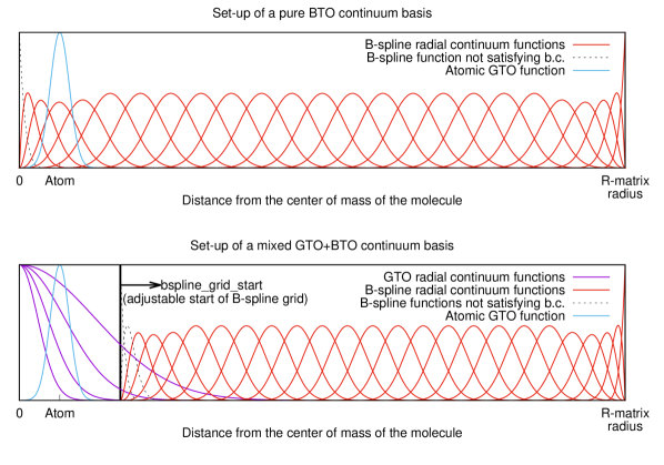
Figure 1: Set-up of the continuum basis in a UKRmol+ calculation. The GTO and the BTO continuum functions centred on the centre of mass can be mixed freely inside the R-matrix sphere. An additional pseudocontinuum basis built from GTOs centred on the centre of mass can also be included (not shown). The parameter bspline_grid_start sets the radial distance for start of the B-spline basis. The B-spline functions plotted using the dashed lines are those not satisfying the boundary conditions, see text.

Table 3: Selected parameters in the &continuum_data namelist in the input for SCATCI_INTEGRALS. Most default values not indicated are set to $-1$.

&continuum_data
min_l	The lowest GTO partial wave to include
max_l	The highest GTO partial wave to include
exponents(:,$l$)	Exponents of the continuum GTOs for
	partial wave $l$
min_bspline_l	The lowest BTO partial wave to include
max_bspline_l	The highest BTO partial wave to include
bspline_grid_start	The radial distance from which the BTOs
	start, see Fig. 1
bspline_order	Order of the B-splines to be included in
	the calculation
no_bspline	The number of radial B-splines in the basis
bspline_indices(1,$l$)	Indices of the first and the last radial B-spline
bspline_indices(2,$l$)	to be included for the partial wave $l$
del_thresh	Deletion thresholds for each irreducible
	representation used in the symmetric
	orthogonalization of the continuum
run_free_scattering	Logical flag that enables the running of a
	free scattering calculation (default:.false.).
min_energy	Minimum scattering energy in Hartree in the
	free scattering calculation
max_energy	Maximum energy in Hartree the free
	scattering calculation
nE	Number of energies between min_energy
	and max_energy

The deletion threshold to be used for each irreducible representation in the symmetric orthogonalization is given by del_thresh (see Section 3.1.5).

If the free scattering calculation is requested using the flag run_free_scattering then the program uses the R-matrix methodology (with the R-matrix radius given in the namelist &target_data) and the target + continuum orbitals as a basis to solve the 1-particle “scattering” problem with zero potential (i.e. with Hamiltonian $H=-\frac{\nabla^{2}}{2}$) and computes the eigenphase sums in each spatial symmetry for a range of energies by matching to spherical Bessel functions at $r=a$. For free scattering, the exact result should be zero eigenphase sums. Therefore the size of the deviations from zero give an idea of the quality of the continuum basis. A rule of thumb for a good continuum representation are eigenphase sums less than or equal to $10^{-2}$ rad. The energy range and grid for this caculations can be adjusted if required using the namelist parameters min_energy, max_energy (in Hartree) and nE. If several free scattering calculations are run in order to tune the continuum basis, this can be made more efficient setting the flag do_two_particle_integrals = .false. in the namelist &process_control, see below.

3.1.3 Namelist pco_data

The basis for the pseudocontinuum is built from even-tempered GTOs centred on the centre of mass. The pseudocontinuum exponents are generated using the formula:

$$\alpha_{j,l}=\alpha_{0,l}\beta_{l}^{(j-1)},\;\;j=1,\dots n_{l},$$ (25)

where the parameters $\alpha_{0,l}$, $\beta_{l}$ and $n_{l}$ correspond to the values PCO_alpha0, PCO_beta and num_PCOs respectively in the namelist &pco_data, see Table 4. Usual values of $\beta_{l}$ range from and 1.1 to 1.5.

Table 4: Parameters in the &pco_data namelist in the input for SCATCI_INTEGRALS. All default values are set to $-1/-1.0$.

&pco_data
PCO_alpha0	Parameters $\alpha_{0,l}$ in Eq (25).
PCO_beta	Parameters $\beta_{l}$ in Eq (25).
num_PCOs	Parameter $n_{l}$ in Eq (25): number of pseudocontinuum
	exponents per partial wave to be generated.
min_PCO_l	The lowest angular momentum for PCOs
max_PCO_l	The highest angular momentum for PCOs
PCO_gto_thrs	Thresholds, per partial wave, for removal of
	exponents of continuum GTOs, see text for details.
PCO_del_thrs	Deletion thresholds for each irreducible representation
	used in the symmetric orthogonalization of the
	pseudocontinuum

If the GTO continuum is included in the calculation too then the exponents of the continuum GTOs for each partial wave are scanned and those greater than or equal to the smallest PCO exponent (minus the value PCO_gto_thrs) in the same partial wave removed. This procedure improves numerical stability of generation of the continuum orbitals. PCO_del_thrs are the deletion thresholds for the symmetric orthogonalization of this basis.

3.1.4 Namelist process_control

Table 5: Selected parameters in the &process_control namelist in the input for SCATCI_INTEGRALS.

&process_control
max_ijrs_size	Maximum size (in MiB) of the auxiliary array
	used during 2-electron integral transformation.
	For distributed (MPI) calculation this value
	represents memory per MPI task. This value
	always has to be set by the user.
do_two_particle_integrals	Logical flag requesting calculation of 2-electron
	integrals (useful for tuning of the continuum
	basis) (default:.true.)
two_p_continuum	Flag requesting calculation of 2-electron
	integrals with two particles in the continuum.
	(default:.false.)
mixed_ints_method	Method to use for evaluation of the mixed
	GTO/BTO integrals (see documentation)
max_l_legendre_1el	Highest partial wave in the Legendre expansion
	of the mixed GTO/BTO nuclear attraction
	integrals
max_l_legendre_2el	Highest partial wave in the Legendre expansion
	of the mixed GTO/BTO two-electron integrals.
calc_radial_densities	Logical flag requesting calculation of the radial
	charge densities of the orbitals included
	in the calculation (default: .false.)
scratch_directory	Path to the scratch directory. Only used
	in case of mixed integrals. If not set the
	auxiliary quantities will be kept in memory (default).
delta_r1	Length in a0 of the elementary
	Gauss-Legendre quadrature used for evaluation
	of the mixed integrals (default: 0.25)

This namelist, see Table 5, controls mainly how the integrals are calculated and how much memory or whether scratch space is requested for some auxiliary quantities needed during the computation of the mixed GTO/BTO integrals. Most importantly, the parameters max_l_legendre_1el and max_l_legendre_2el control the highest partial wave included in the Legendre expansion of the Coulomb potential when calculating the mixed GTO/BTO integrals. The minimum sensible numbers for these quantities is twice the value of the highest (pseudo)continuum angular momentum included in the calculation. Careful convergence checks of the final results with respect to these parameters are recommended. The length of the Legendre expansion significantly affects both the computational time and the memory requirements of the calculation. Values as high as $75$ have been used in calculations [38]. The flag calc_radial_densities is useful for testing whether the R-matrix radius chosen is sufficiently large.

3.1.5 Orbital orthogonalization

It is a requirement of the UKRmol+ suite that all the orbitals used form a single orthonormal set; orthogonalization steps are therefore required. The target orbitals are usually orthonormal on input but as the first step they are preemptively reorthogonalized using the Gram-Schmidt method. The flow of the orthogonalization process is shown in or ig. 2.

Figure 2: Workflow of the orbital orthogonalization. The steps 2 and 3 are only performed if the basis includes, respectively, the corresponding pseudocontinuum atomic orbitals (PCOs) and continuum orbitals (COs). The dashed arrows represent the workflow in the case PCOs and/or COs are not included in the calculation.

In a standard scattering calculation only the target and the continuum bases are included and only steps 1 and 3 from Fig. 2 are performed. In this case the Gram-Schmidt orthogonalization of the continuum basis with the target orbitals (step 3a) leaves the latter unchanged. The second (step 3b), symmetric orthogonalization [39], ensures that the continuum orbitals (now expanded in a a linear combination of the continuum and atomic bases) are orthogonal among themselves.

Deletion thresholds for each irreducible representation are provided by the user for the symmetric orthogonalization in the namelist &continuum_data: those continuum orbitals with eigenvalues of the overlap matrix smaller than this threshold are deleted. The appropriate value for this threshold varies depending on the type of continuum basis used and typically lies in the range $10^{-7}$ to $10^{-9}$ for a pure GTO continuum basis. Lowering the deletion threshold corresponds to decreasing the relative precision of the transformed integrals and therefore increasing the risk of running into numerical linear dependence problems when diagonalizing the inner-region Hamiltonian. Increasing the deletion threshold, on the other hand, means more continuum functions are deleted from the basis, lowering the quality of the continuum description. The numerical problems can be avoided (and the deletion thresholds set to a value low enough ensuring no continuum orbitals are deleted) by compiling and running SCATCI_INTEGRALS in quadruple precision albeit at the expense of a much increased compute time (see below for details). For this reason quad precision calculations have only been performed using pure GTO continuum in which case all integrals have analytic form. In calculations using either a mixed GTO+BTO or a pure BTO continuum the deletion thresholds can be set to a much higher value (typically $10^{-5}$). The higher value of the deletion threshold means that the numerical linear dependence problems are essentially absent in this case (as expected for a B-spline basis) thus removing the need to run the integral calculation in quad precision.

If a pseudocontinuum basis is included in the calculation, additional orthogonalization steps are required: this basis needs to be orthogonalized to the target orbitals and among itself (step 2) before the continuum is orthogonalized to the joint target + pseudocontinuum basis (step 3). The deletion threshold to be used for the symmetric orthogonalization of the pseudocontinuum orbitals is provided in the namelist &pco_data and is usually set to a relatively high value of about $10^{-4}$; some pruning of the continuum orbitals may also be necessary in this case to avoid problems with linear dependence.

3.1.6 Integrals evaluated by SCATCI_INTEGRALS

The one-electron integrals are defined as:

$$\langle a|\hat{O}|b\rangle=\int d^{3}ra(\mathbf{r})\hat{O}b(\mathbf{r}),$$ (26)

where $\hat{O}$ is a one-electron operator and $a$, $b$ are either atomic or molecular orbitals. SCATCI_INTEGRALS generates by default the following types of 1-electron integrals:

overlap: $$\hat{O} =1,$$ (27)

kinetic energy: $$\hat{O} =-\frac{\nabla^{2}}{2}+L,$$ (28)

nuclear attraction: $$\hat{O} =\sum_{k=1}^{Nuclei}-\frac{Z_{k}}{|\mathbf{r}-\mathbf{R}_{k}|},$$ (29)

multipole: $$\hat{O} =S_{l,m}(\mathbf{r}),\ \ l\leq 2,$$ (30)

1-electron Hamiltonian: $$\hat{O} =-\frac{\nabla^{2}}{2}+L+\sum_{k=1}^{Nuclei}-\frac{Z_{k}}{|\mathbf{r}-\mathbf{R}_{k}|},$$ (31)

where $L=\frac{1}{2}\delta(r-a)\frac{d}{dr}$, the Bloch operator, is included only if both $a$ and $b$ are continuum functions (the multielectronic form of this operator was introduced in Eq. (10)). The two-electron (Coulomb) integrals are:

$$\langle ab||bc\rangle=\int d^{3}ra(\mathbf{r}_{1})b(\mathbf{r}_{1})\frac{1}{|\mathbf{r}_{1}-\mathbf{r}_{2}|}c(\mathbf{r}_{2})d(\mathbf{r}_{2}).$$ (32)

Depending on the particular combination of the functions $a$, $b$, $c$, $d$ the integral will belong in one of six unique classes:

$$\langle TT||TT\rangle,\langle TC||TT\rangle,\langle TC||TC\rangle,\langle CC||TT\rangle,\langle CC||CT\rangle,\langle CC||CC\rangle,$$

where $T$ and $C$ stand for atomic/molecular orbitals representing the target (or pseudocontinuum) and continuum respectively. The last two classes of integrals (with at least three $C$-type functions) are only needed in calculations where two particles are in the continuum. Since UKRmol+ supports only calculations with one particle in the continuum these integrals are not generated by default. However, they can be generated setting the variable two_p_continuum = .true. in the namelist &process_control, see Table 5 (Section 3.1.3). In the current version this option is not available if the basis contains BTOs but it will be implemented in the future.

In the case of the class $\langle CC||TT\rangle$ and the one-electron integrals $\langle C|C\rangle$, when on input the R-matrix radius is a$>0$, the atomic integrals are computed only over the interior of the R-matrix sphere with radius a. The other classes of integrals are computed over all space unless the continuum functions are all BTOs.

GBTOlib [10] uses object oriented features from the Fortran 2003 standard and involves distributed and shared-memory parallelization to evaluate the 1-electron and 2-electron integrals defined above. The program proceeds by generating first the 1-electron and 2-electron integrals in the atomic basis and then transforming them into the molecular basis. The whole calculation is performed in core (perhaps with exception of the mixed integrals, see namelist &process_control). Only the final array of the transformed molecular integrals is saved to disk (along with the full basis set information). It is the integrals in the molecular basis which are used by the other programs in the UKRmol+ suite.

A very useful feature of the GBTOlib is that it can be compiled and run in quad precision: this does not amount to a mere recompilation using a different kind parameter but to actual evaluation of the integrals with increased relative precision (i.e. using more accurate versions of special functions and higher-order quadratures which evaluate to near-full quad precision accuracy). This feature has been used extensively over the last couple of years mostly in photoionization calculations requiring large GTO continuum bases, see e.g. [40, 41] but also in calculations with molecular clusters [42, 43] and biomolecules [44].

In the current release version of GBTOlib distributed evaluation is not allowed when mixed GTO/BTO 2-electron integrals are required: only shared-memory parallelism is available for this type of calculation. However, distributed evaluation of these integrals will be implemented in the next major release of the code along with the option to save the atomic integrals to disk.

3.2 CONGEN

The program CONGEN generates the configuration state functions (CSF) that will be used in building the N or N+1 electron wavefunctions. As such, input to this program defines to a large extent the model that will be used in the description of the scattering/photoionization process; it is in the input required by CONGEN that the SE, SEP, CC and RMPS approximations are most different. This can make the input of CONGEN complex to generate.

CONGEN does not require any input (data) files generated by other programs. The only information needed from earlier parts of the calculation is the number of target orbitals (specified by the parameter nob0, see Table 6) belonging to each irreducible representation and the total number of orbitals resulting from the orthogonalization of the continuum to the bound orbitals (again, for each irreducible representation and specified by the parameter nob). This is provided by the user in the input, together with detailed information specifying the construction of the CSF. When the projectile is a positron, the number of orbitals needs to be doubled: the same orbitals that can be occupied by the electrons will have a differnet index when they are occupied by the positron.

Two namelists are required for CONGEN: &state and &wfngrp. Only one occurrence of the former is allowed, but several instances of the second one may be required to define all the CSFs to be generated.

Table 6: Selected parameters in the &state namelist in the input of CONGEN. The storage size and memory allocation is indicated in words.

&state
iscat	Indicates whether N, if set to 1 (no phase correction) or N+1
	electron calculation, if set to 2 (phase correction) (default:0)
	(see next section for details on the phase correction)
qntot	Triplet that indicates the space-spin symmetry of CSFs
	generated
nelect	Total number of electrons
megul	File unit for the output CSFs (default: 13).
nob	Total number of orbitals for each irreducible representation
nob0	NUmber of target orbitals for each irreducible representation
nrefo	Number of quintets in reforb
reforb	Quintets that describe the reference determinant
lndo	Controls assignment of temporary storage (default: 5000)
lcdo	Controls assignment of temporary storage (default: 500)
nbmx	Memory allocation for CSFs generation (default: 2000000)
iposit	Lepton charge flag (default; 0, indicates electron; 1, positron)

CONGEN generates CSFs as differences from a reference configuration. This configuration, specified using nrefo and reforb in the namelist &state, should have the correct space-spin symmetry (given by qntot), but does not need to be physically meaningful. However, use of a ‘sensible’ configuration is recommended, as the number of differences that need to be stored will be reduced. The iposit flag in the namelist &state indicates whether the calculation is for a positron or electron in the continuum.

When CONGEN is used for the N+1 system, the CSFs to be generated are those described by the two terms in Eq. (21). This means that there are two types of CSFs (a) those which correspond to the product of a target state (whose symmetry must be given by the parameter qntar, see Table 7) and a continuum orbital and (b) those L² CSFS where all electrons occupy target orbitals. There are some rules about the order in which these configurations must be generated, namely: (1) all CSFs of the target plus continuum type must precede the L² ones and (2) all CSFs associated with a single target symmetry, and hence value of qntar, must be grouped together and generated in a canonical order which is used in all parts of the calculation (eg for the target only calculation). As the first step in the SCATCI algorithm [45] is based on the use of Yoshimine’s prototype configurations [46], CONGEN only actually generates CSFs of the first type (a) corresponding to the first two continuum orbitals for each scattering symmetry. Note that it is possible to treat CSFs of the form target times virtual orbital in same fashion as the target times continuum orbitals, see Ref. [27] for a discussion of this.

Table 7: Selected parameters in the &wfngrp namelist in the input of CONGEN.

&wfngrp
qntar	Space-spin symmetry of the target states being coupled to
nelecg	Number of ’movable’ electrons
nrefog	Number of reforg quintets needed to describe movable electrons
reforg	Quintets which describe the movable electrons
ndprod	Number of sets of orbitals into which the electrons will be
	distributed
nelecp	Number of electrons to be distributed into each set of orbitals
nshlp	Number of pqn triplets needed to describe each set of orbitals
pqn	Triplets that describe each set of orbitals in which the movable
	electrons will be distributed
mshl	For each pqn, the irreducible representation the described
	orbitals belong to

The namelist &wfngrp contains the information that specifies the CSFs to be built. The ‘movable’ electrons are those that are going to be promoted from the reference configuration to generate the desired CSFs. If all the CSFs to be generated contain the same set of core electrons (in other words, the same set of doubly occupied orbitals), then the number of movable electrons, specified by nelecg in the &wfngrp namelist, will be smaller than the total number of electrons of the system. In that case, nreforg and reforg will specify the orbitals in the reference configuration from which electrons are going to be promoted (if nelecg=nelect then reforg and reforb will specify the same configuration). The CSFs themselves are specified using th parameters nelecp, nshlp, pqn and mshl.

The details of the syntax for the qntot and qntar triplets, reforb and reforg quintets as well as the pqn triplets can be found in the documentation of CONGEN. Special care should be exercised in the case of positron scattering because of the doubling up of the orbital labels.

CONGEN runs serially and does not require linking to any external libraries for compilation. The program needs to be run for each space-spin symmetry for which CSFs are required. It was initially written in Fortran 66 as part of the Alchemy I suite [47] and recently modernized to use Fortran 95 and 2003 features.

3.3 SCATCI and MPI-SCATCI

The main task performed by UKRmol-in is the construction and diagonalization of a Hamiltonian matrix in order to obtain the bound and (discretized) continuum wavefunctions describing the molecule + free (N+1) electron system. This task uses an algorithm [45] especially designed to efficiently construct Hamiltonian matrices with the close-coupling structure of Eq. (21); this is carried out by either SCATCI or MPI-SCATCI [48]. The latter is a parallel implementation of a re-engineered version of the algorithm employed by SCATCI that makes use of modern computer architectures and has added functionality (see Section 6).

Table 8: Diagonalization modes and methods of SCATCI and MPI-SCATCI depending on the number of requested eigenvectors and library used. Except for the Davidson diagonalization routine [49], all other depend on external libraries: LAPACK, Arpack [50], ScaLAPACK [51], or SLEPc [52]. The classifications “few” and “many” is automatically assigned using built-in percentages of requested eigenpairs and the size of the Hamiltonian. The diagonalization method can also be specified manually, in the &cinorn namelist.

eigenvectors	SCATCI/serial MPI-SCATCI	parallel MPI-SCATCI
“few”	Davidson	Krylov-Shur (SLEPc)
“many”	Arnoldi (Arpack)	Krylov-Shur (SLEPc)
all	dense (LAPACK)	dense (ScaLAPACK)

In typical situations, SCATCI/MPI-SCATCI require two files on input: the CSFs constructed by CONGEN and the molecular integrals file generated by SCATCI_INTEGRALS. These files must be generated specifying the same number of target orbitals. The calculated eigenvectors and eigenvalues (eigenpairs) are either written to a new file as a first “dataset”, or appended to an already existing file as another “dataset”.

As with CONGEN, SCATCI/MPI-SCATCI is executed for each space-spin symmetry independently and operates either in target or in scattering mode. In the case of diagonalization of the scattering, N+1-electron Hamiltonian, SCATCI can either calculate the target, N-electron eigenstates needed in Eq. (21) on its own, or read them from a file produced before by diagonalization of the target Hamiltonian (nftg in namelist &input). The former method is sufficient for scattering calculations of integral cross sections. The latter method is needed to ensure phase consistency [53] across all irreducible representations of the $(N+1)$-electron system; the same target eigenstates are supplied to all independent diagonalizations of the scattering Hamiltonians. If this was not done, some of the independently on-the-fly re-calculated target eigenstates for two different scattering irreducible representations might end up with different phases, introducing random relative signs to the obtained coefficients $c_{ijk}$ in Eq. (21) and causing errors in the calculation of matrix elements between the (N+1)-electron eigenstates. This is important in calculations of angular distributions in electron impact electronic excitation [54, 55] and is crucial when using CDENPROP for photoionization calculations (see below).

Depending on the setup of the calculation, SCATCI/MPI-SCATCI may either produce all eigenpairs, or just the requested number of lowest-lying ones. Target calculations usually only request a few low-lying states. Traditional R-matrix calculations require all solutions of the N+1 inner region Hamiltonian; however, when the Hamiltonian is very large the partitioned R-matrix approach provides an alternative which only requires a subset of the solutions [56] (this approach, available in the UKRmol suite, will be implemented for scattering calculations in a forthcoming release of UKRmol+). The number of eigenpairs to be calculated determines the choice of diagonalization method, not all of which are available if the programs are not compiled with all optional libraries; Table 8 summarizes the choices and availability.

Table 9: Selected members of the SCATCI and MPI-SCATCI &input namelist. Entries labelled with an asterisk are only used in scattering runs. Detailed information is provided in the program documentation.

&input
icitg	Indicates target (= 0, default) or scattering (= 1), i.e.
	with target contraction, run.
iexpc*	Expand (= 1) continuum in scattering prototype CSFs
	(default: 0).
idiag	Hamiltonian evaluation flag (see documentation);
	often 1 (default) for target, 2 for scattering.
nfti	File unit with molecular integrals (default: 16).
nfte	File unit for Hamiltonian output (default: 26).
megul	File unit with CONGEN generated CSFs (default: 13).
ntgsym*	Number of different target space-spin symmetries
	included in the Hamiltonian construction
numtgt*	Number of target eigenstates per ntgsym
mcont*	$M$-value of continuum orbitals per target ntgsym
notgt*	Number of continuum orbitals used per target ntgsym
nftg*	File unit for input target eigenstates; if 0, not read
	(default: 39)
ntgtf*	For each target state used in CONGEN, index of the set
	in nftg containing it (default: 0)
ntgts*	For each target state used in CONGEN, sequence number
	of the state within the ntgtf set

SCATCI/MPI-SCATCI require two namelists in its standard input, called &input and &cinorn. The first one defines the construction of the Hamiltonian, while the second one specifies details of the diagonalization method and how and where the produced eigenpairs will be stored. Tables 9 and 10 summarize the most important members of the two namelists.

When a target calculation is run, the namelist input is rather simple: in &input one should make sure to indicate the correct unit for the CONGEN output (using megul) and in &cinorn one should indicate how many states (eigenpairs) of that particular space-spin symmetry are requested (nstat) and which set they will be stored in (nciset). In the case of an N+1 calculation, the parameters in the &input namelist will specify how many target states per space-spin symmetry (numtgt) and how many space-spin symmetries (ntgsym) are being used to build the wavefunctions; mcont indicates the symmetry of the continuum orbitals each set of target states is coupled to in order to generate eigenfunctions of the appropriate (N+1) symmetry and notgt indicates how many of these orbitals there are.

MPI-SCATCI shares most serial capabilities with SCATCI when executed in a single process, and also supports parallel execution based on MPI. In the latter case the construction of the Hamiltonian matrix is distributed among all processes and the diagonalization performed by the appropriate parallelized SLEPc or ScaLAPACK subroutine. On top of that, MPI-SCATCI allows concurrent diagonalization of many Hamiltonians in one run, which is particularly advantageous when only matrix elements between the calculated eigenstates (possibly of different irreducible representations) are desired rather than the states themselves. Concurrent in-core diagonalization then avoids the need of writing the eigensolutions to disk and enables immediate fast in-memory processing once all diagonalizations finish.

Table 10: Selected members of the SCATCI and MPI-SCATCI &cinorn namelist.

&cinorn
igh	Force iterative (= 0 Davidson, =-1 Arpack) or dense (= 1)
	diagonalization method.
nstat	Number of eigenvectors to be calculated (default: 0 = all).
nftw	File unit for output of eigenvectors (default: 25).
nciset	Output dataset index in nftw (default: 1).
vecstore	Indicates whether all coefficients of the expansion, Eq. (21),
	are to be saved (=0, default) or only those that multiply
	configurations of the type ’target state + continuum’ (=1).

Table 11: Members of MPI-SCATCI optional input namelist &outer_interface.

&outer_interface
write_amp	If .true., produce boundary amplitudes file (unit 21).
write_dip	If .true., produce transition dipoles file (unit 624).
write_rmt	If .true., produce RMT input file molecular_data.
rmatr	R-matrix radius, for evaluation of boundary amplitudes.
ntarg	(See SWINTERF, Table 14.)
idtarg	(See SWINTERF, Table 14.)
delta_r	(See RMT_INTERFACE, Table 15.)
nfdm	(See RMT_INTERFACE, Table 15.)

To this end, MPI-SCATCI features some advanced wave function post-processing capabilities which can be used as a simplified alternative to CDENPROP_ALL, SWINTERF and RMT_INTERFACE described below: it can directly evaluate the permanent and transition dipole moments between the eigenstates or produce the input for UKRmol-out. These additional stages are controlled by an optional namelist &outer_interface summarized in Table 11. The outer interface built into MPI-SCATCI takes advantage of MPI parallelization and carries out all matrix multiplications needed to evaluate wave function properties and amplitudes in parallel, using the ScaLAPACK subroutines. This also has the advantage of evenly distributing the memory requirements, which might otherwise become insurmountable for the serial codes.

3.4 DENPROP

The program DENPROP calculates the permanent and transition dipole and quadropole moments between states of the target (N-electron system). In order to do this, the program calculates density matrices. In addition, the program can determine the spherical polarizability of the target molecule [33] using the perturbative sum-over-states formula; this quantity can be used to determine approximately how well polarization effects are being modelled in the calculation [30, 31]. DENPROP produces as its main output a target property file that is used by the interface programs. This file contains all the permanent and transition moments as well as the energy of the target states (read in from the output of SCATCI/MPI-SCATCI).

Table 12: Selected parameters in the DENPROP &input namelist.

&input
nftg	File unit number for the output of SCATCI/MPI-SCATCI
	(default: 25)
ntgt	Number of different space-spin symmetries to be read in
	from nftg
ntgtf	Set number in unit nftg in which the eigenvectors for a
	specific space-spin symmetry are found (default: 1,2,3, …)
ntgs	Sequence number, within a specific ntgtf, of the first
	eigenvector to be used (default: 1 for all ntgtf)
ntgtl	Sequence number, within a specific ntgtf, of the last
	eigenvector to be used (default: 1 for all ntgtf)
nftsor	File unit numbers of the CONGEN output files for each
	space-spin symmetry
ipol	Flag for the calculation of the polarizability (default: 1, calculate)
zlast	Set to .true. to save CPU time (default: .false.)

DENPROP requires as input the property integrals determined by SCATCI_INTEGRALS, the target CSFs generated by CONGEN and the wavefunctions obtained from SCATCI or MPI-SCATCI, respectively. Further input to DENPROP is provided via the namelist &input; the main parameters are given in Table 12. This namelist provides information on which target states and of which symmetry the moments are to be determined for, as well as which intermediate files contain the relevant input data.

The program CDENPROP_ALL (described in he next section) can be used instead of DENPROP, providing the same input. It is expected that, in the medium term, CDENPROP will replace DENPROP, possibly with the exception of very large target calculations for which the algorithms used by DENPROP are more suitable.

3.5 CDENPROP and CDENPROP

The program CDENPROP constructs the 1-particle reduced density matrix represented in the close-coupling basis of Eq. (21). For a concise notation we rewrite Eq. (21) in the more compact form

$$\Psi_{k}=\sum_{i}c_{ki}\Phi_{i}$$ (33)

where $\Phi_{i}\in\{A\Phi^{N}_{m}\eta_{n},\Phi^{(N+1)}_{p}\}$. The expressions $A\Phi^{N}_{m}\eta_{n}$ and $\Phi^{(N+1)}_{p}$ indicate the two types of terms used in Eq. (21). The 1-particle density matrix is then

$$\rho_{ij}(\mathbf{x}_{N+1})=(N+1)\int{\Phi}_{i}{\Phi}^{*}_{j}\,\mathrm{d}^{3}\mathbf{x}_{1}\dots\mathrm{d}^{3}\mathbf{x}_{N}$$ (34)

and can be used to calculate the transition moment matrix $\mathcal{M}$,

$$\mathcal{M}_{ij}=\int\mu\rho_{ij}\,\mathrm{d}^{3}\mathbf{x}\,,$$ (35)

and finally the transition moments, i.e. elements of the multipole (dipole,$\mu$, quadrupole, etc.) operators, between the inner region wavefunctions,

$$M_{kl}=\langle\Psi_{k}|\mu|\Psi_{l}\rangle=\sum_{kl}c_{ki}c_{lj}\mathcal{M}_{ij}\,.$$ (36)

When the coefficients for the bound $(N+1)$-electron system are supplied on input ($A_{k}(E)$ in Eq. (20)), CDENPROP can also evaluate the Dyson orbitals (overlaps of neutral and ionic bound state wave functions)

$$D_{ij}(\mathbf{x}_{N+1})=\sqrt{N+1}\int\Phi_{i}^{N}\Psi_{j}^{N+1*}\,\mathrm{d}^{3}\mathbf{x}_{1}\dots\mathrm{d}^{3}\mathbf{x}_{N}$$ (37)

and write them to disk in the Molden format. For a detailed description of the code and algorithms used see [57].

The UKRmol+ suite contains two programs with similar functionality that are based on CDENPROP code: CDENPROP itself and CDENPROP_ALL. The first one calculates transition dipole and quadrupole moments between a chosen number of N+1-electron states belonging to two identical or distinct space-spin symmetries. This is useful for photoionization, where transition moments are usually calculated between the initial ground state of the neutral molecule and states from only those symmetries coupled to it by the dipole operator. Table 13 contains the most frequently used namelist parameters for CDENPROP. The first of the two numbers assigned to the parameters lucsf, lucivec, nstat and nciset correspond to the ground (“ket”) state, while the second one corresponds to the final (“bra”) states. See also the Section 5 a for detailed description of the photoionization calculations.

Table 13: Selected parameters in the CDENPROP input namelist.

&deninp
luprop	Input file unit with the molecular integrals (default: 17).
lutdip	Input file unit with target properties (default: 24).
lutargci	Input file unit with target eigenstates (default: 26).
lupropw	Output file unit for moments (default: 624).
lucsf	Two input file units containing ket and bra CSFs.
lucivec	Two input file units containing ket and bra eigenstates.
nstat	Numbers of ket and bra states to consider (0 = all).
nciset	Datasets in lucivec to read states from.
numtgt	Number of target states per space-spin symmetry as used
	in SCATCI.

On the other hand, CDENPROP_ALL calculates matrix elements for transitions between all pairs of states in all symmetries provided, not limited to two of them. As such, it can act as an alternative to DENPROP, when applied on target eigenstates. When applied on scattering eigenstates, it may produce a massive amount of data, currently only needed by RMT (see below). The input namelist for CDENPROP_ALL is identical to that of DENPROP, except that in the case of evaluation of (N+1)-electron properties, it also needs to contain the entry numtgt explained in Table 13.

3.6 Interfaces

The inner region wave functions obtained by UKRmol+, or their properties, can be used to provide input for other suites or programs. The interfaces SWINTERF and RMT_INTERFACE are responsible for extracting useful data from the inner region solutions that are passed further.

Once the interfaces have run, the output files from the target and inner region calculations can be deleted and further outer region/RMT calculations can be run using the interfaces output.

3.6.1 SWINTERF

SWINTERF interfaces with UKRmol-out, the suite of outer region codes that perform the R-matrix propagation to obtain K-matrices and, from these, various scattering quantities: cross sections, eigenphase sums, resonance parameters, etc. It is also used by RMT_INTERFACE (see the next section).

The information required by the program is: the target properties (generated by DENPROP and including the energies and permanent and transition moments), the raw boundary amplitudes (see A) produced by SCATCI_INTEGRALS and the inner region eigenpairs, generated by SCATCI or MPI-SCATCI.

The namelist &swintfin is the only one needed by the program. The main parameters provided via this namelist are summarized in Table 14.

Table 14: Selected parameters in the &swintfin namelist in the input of SWINTERF.

&swintfin
mgvn	Symmetry (irreducible representation) of the scattering
	wavefunction.
stot	Spin multiplicity of the scattering wavefunction.
ntarg	Number of target electronic states to be included in
	the outer region calculation
idtarg	Array specifying which ntarg target states to select
luamp	Input file unit containing the raw boundary amplitudes
	(default:22)
luci	Input file unit containing the N+1 eigenpairs (default:25)
lutarg	Input file unit containing the target data (default:24)
luchan	Output file unit containing the channel information
	(default: 10)
lurmt	Output file unit for the R-matrix poles, boundary
	(default: 21)
	amplitudes and coefficients of the multipole potential
icform	Format flag for channel data file, ’F’ for formatted, ’U’ for
	unformatted (default)
irform	Format flag for R-matrix data file, ’F’ for formatted, ’U’
	for unformatted (default)
nvo	Number of virtual orbitals used ’as continuum’ in CONGEN,
	also used to skip target states.
rmatr	R-matrix radius
ismax	Maximum multipole retained in expansion of long range
	potentials (default: 2)
iposit	Controls the charge sign for asymptotic potential
	interactions (=0, default, for electrons; =1 for positrons)
last_coeff_saved	Index of the last CI coefficient of all eigenvector
	saved by SCATCI/MPI-SCATCI.

As is the case for the construction and diagonalization of the N+1 Hamiltonian, the outer region calculation is performed separately for each space-spin symmetry of the N+1 system; this symmetry needs to be indicated on input using mgvn and stot. The user should also indicate how many (ntarg) and which (idtarg) target states are to be considered (for the definition of the scattering channels) in the outer region: it is possible, and sometimes desirable, to use a smaller number than those included in the inner region calculation as this reduces the number of scattering channels and therefore the computational cost of the outer region calculation. It is inadvisable, however, to exclude energetically open states.

The radius of the R-matrix sphere (rmatr) needs to be provided too as it is used later on to calculate the R-matrix elements following Eq. (18). The user can also decide (using ismax) whether dipoles or both dipoles and quadrupoles are retained for the expansion of the projectile-target interaction potential in the outer region. In addition, if virtual orbitals are used ’as continuum’ in CONGEN (see Section 3.2) the number of these has to be specified, for each target state, using the vector nvo. Finally, iposit indicates whether the projectile is an electron or a positron.

SWINTERF produces two output files: one containing the channel data and another containing the raw boundary amplitudes (see A) required for the construction of the R-matrix, and the coefficients of the coupling potentials. We note that these two files also provide a convenient medium for archiving the results of a calculation for use in possible future runs.

3.6.2 RMT_INTERFACE

The RMT_INTERFACE prepares the molecular input file for the RMT package [13]. RMT solves the time-dependent Schrödinger equation of the molecule in a variable electric field, allowing for ionization of one electron into the continuum. Like UKRmol+, RMT splits the configuration space into an inner, fully correlated, region and an outer region where a one-electron channel expansion is used. The connection between these two regions is realized by an overlap that still counts as the inner region. However, this overlap of the two regions needs to be already free of bound orbitals, which means that when preparing input for RMT the inner region (i.e. the R-matrix radius) has to be somewhat larger than the smallest physical one typically used when dealing with standard stationary scattering or photoionization. The continuity of the inner and outer wave function is maintained using the amplitudes $w_{ik}(r_{j})$ of the inner-region eigenstates $i$ in the outer region channel $k$; these are similar to the boundary amplitudes defined in Eq. (19) but they are evaluated at several uniformly spaced radii $r_{j}$ still within the R-matrix sphere, see Fig. 3. The number of these extra evaluation radii (nfdm in the namelist &rmt_interface_inp) and their spacing (delta_r) must be consistent with the RMT setup. The parameter nfdm is related to the finite difference order $D$ used in the outer region of RMT and to the time propagation order $Q$ as nfdm $=D(Q+1)$. While $D$ is a compile-time constant in RMT and set to 2 (resulting in a 5-point discretization scheme), the propagation order $Q$ is an input parameter to RMT. A typical value is $Q=8$, which results in the recommended nfdm = 18. The spacing between the evaluation radii needs to be equal to the finite difference discretization of the RMT outer region, and is usually in the $0.1\,\mbox{a${}_{0}$}$ range.

Figure 3: Parameters for finite-difference discretization of the inner wave function in RMT. Each number $j$ indicates a sphere of radius $r_{j}$.The physical R-matrix radius (i.e. fully containing the target orbitals) must be smaller than or equal to the radius 1.

RMT_INTERFACE also correctly transforms boundary amplitudes between the UKRmol+ and RMT normalization conventions which differ by a factor of $\sqrt{2}$; RMT expects $w_{ik}$ such that Eq. (18) becomes

$$R_{ij}(a,E)=\frac{1}{2a}\sum_{k}\frac{w_{ik}^{RMT}(a)w_{jk}^{RMT}(a)}{E_{k}-E}.$$ (38)

Table 15: Parameters in the RMT_INTERFACE input namelist &rmt_interface_inp.

&rmt_interface_inp
nfdm	Number of in-sphere boundary evaluation radii…
delta_r	… and spacing between them in atomic units.
lutarg	Input file unit containing the target data (default: 24).
lunp1	Input file unit containing the (N+1)-electron
	moments (default: 667).
n_symmetries	Number of &swintfin namelists to process.

The program RMT_INTERFACE builds on SWINTERF, which is—under the hood—automatically called once for every (N+1)-electron spin-symmetry included in the calculation to obtain the channel information and the amplitudes at all requested radii. The input file follows this need and must contains enough copies of the SWINTERF input namelist &swintfin, one for each space-spin symmetry required. Apart from these namelists, the input for RMT_INTERFACE contains only a short additional namelist &rmt_interface_inp, which is expected at the beginning of the standard input (before all &swintfin namelists) and whose parameters are summarized in Table 15.

The output of RMT_INTERFACE is the binary stream file molecular_data directly readable in RMT.

4 Scattering calculations

A typical workflow for the part of a scattering calculation using the UKRmol-in programs together with the interface is illustrated in Fig. 4.

Figure 4: Workflow for the inner region and interface parts of a scattering calculation. Red indicates the molecular orbital (Molden) file produced by a compatible quantum chemistry package, white are intermediate files, green are the final outputs. Programs in the orange box need to be executed for all the required (target) space-spin symmetries and those in the grey box for all (scattering) space-spin symmetries. Each program needs also its own input namelist(s) not shown in the diagram. The numbers next to individual programs indicate the typical execution order.

For SE and SEP calculations, the determination of the target properties is straightforward and the only significant choice is that of the basis set. For the inner region part of the calculation, the main choice is that of the virtual orbitals to be used in the construction of the L² functions (see Section 2). The R-matrix radius will be given by the orbitals used and can be checked with SCATCI_INTEGRALS (using the option calc_radial_densities) and the choice of the type of continuum basis is linked to it and the scattering energies to be investigated. Since scattering calculations are normally performed for energies up to no more than few eV higher than the ionization threshold, the energies to be covered are normally up to around 20 eV. This means that, in general, for R-matrix radii smaller than 15 a₀, GTOs only will suffice (see, for example, [58, 59]). Use of BTOs only as well as mixed bases have been tested for diatomic and triatomic targets [38, 60]. The choice of type of continuum basis is independent of the scattering model being used. The interface (SWINTERF) calculation is also straightforward, with the only significant choice being whether to use only dipoles or include quadrupole moments too in the expansion of the static multipole molecular potential.

For CC calculations, the choices in terms of describing the target are several, and more difficult to make. The first choice is that of the orbitals to be used: it is now customary to use State-Averaged CASSCF orbitals generated by an external Quantum Chemistry code. An active space, and the states to be averaged need to be specified in the input to those codes. The former choice is usually limited, due to the requirement for balance [24] between the N and N+1 electron wavefunctions, by the number of N+1 electron CSFs that a specific active space will generate; this is particularly the case for molecules with large polarizabilites that require the use of several types of L² functions.

The states to be averaged will normally be a subset of those included in the scattering calculation: usually, a few active spaces and state-averaging schemes are tested and the excitation thresholds and the ground state energy and dipole moment (if the molecule is polar) of the target are checked to decide on the best choice.

We note that the symmetry of the target molecules is critical here: for a molecule with no symmetry, the size of the Hamiltonian to diagonalize is given by the total number of CSFs. For a molecule belonging to the D_2h this number will be split roughly equally between the 8 irreducible representations leading to 8, much smaller, Hamiltonian blocks that need to be diagonalized (for this reason, it can be convenient to study higher symmetry molecules as models for more complex targets [61]).

For the inner region calculation, one needs to choose, once again, the R-matrix radius and continuum basis to use: the same considerations as for SE/SEP calculations apply here. Under certain conditions (e.g. large number of bound orbitals, high-quality continuum description involving BTOs, large R-matrix radii) SCATCI_INTEGRALS can become the computationally heaviest part of a calculation.

In terms of the target states to include in the construction of the N+1 electron wavefunctions, it is customary to use all those that are energetically accessible in the scatting energy range of interest (if pseudostates are used, other considerations, like a good description of polarization effects, should be taken into account).

Increasing the number of target states does not contribute to the size of the Hamiltonian as much as increasing the number of L² function (by, for example, choosing a bigger active space). This increase, however, will have an effect in the outer region calculation since the number of channels is linked to the number of target states.

4.1 UKRmol-out

A workflow for the part of a scattering calculation using the UKRmol-out programs is illustrated in Fig. 5. Unlike the target and inner region part of the calculations, where most programs are run in a predetermined sequence, which UKRmol-out programs are run depends on the scattering data the user requires.

Figure 5: Workflow for the outer region of a scattering calculation. The channel information and boundary amplitudes produced by the inner region (Fig. 4) are used as input. This whole workflow (or its subset if not all output data are needed) is repeated for all space-spin symmetries relevant for the calculation. The color coding is as in Fig. 4.

The first step in most outer region calculations (the most significant exception is the study of bound states; see next section) is the propagation of the R-matrix from the R-matrix boundary to an asymptotic region where, by matching to asymptotic expressions [20], the K-matrices can be determined. It is this step, performed by the program RSOLVE, that becomes resource consuming when a large number of channels are included in the calculation. For this reason, a parallelized version of it, MPI-RSOLVE is also available (it requires identical input to the serial version). In addition, the highly efficient, parallel program PFARM [19] can also be used for large calculations to perform the propagation and generate the K-matrices; the suite provides an interface program, PFARM_INTERFACE, that ensures the inner region data is in the correct format for input to PFARM. The namelist of RSOLVE/MPI-RSOLVE is described in Table 16. For large calculations it may be desirable to compute directly the T-matrices for the selected transitions of interest rather than full K-matrices: additional namelist variables available only in MPI-RSOLVE allow for this mode to be selected, see source code.

Table 16: Selected namelist variables in the namelist &rslvin for RSOLVE.

&rslvin
mgvn	Symmetry (irreducible representation) of scattering system
	(as in SWINTERF)
stot	Spin multiplicity of the scattering system (as in
	SWINTERF)
nerang	Number of subranges of scattering energies
nescat	Number of input scattering energies in each subrange
einc(1,$i$ )	Initial energy in subrange $i$
einc(2,$i$ )	Energy increment (step) in subrange $i$
range ienut	Units in which scattering energies are input; 1= Ryd
	(default), 2= eV
luchan	Input file unit containing the channel information
	(default: 10)
lurmt	Input file unit for the R-matrix poles, boundary amplitudes
	and coefficients of the multipole potential (default: 21)
lukmt	Output file unit for the K-matrices
icform	Format flag for input channel data file, ’F’ for formatted,
	’U’ for unformatted (default)
ikform	Format flag for output K-matrix data file, ’F’ for formatted,
	’U’ for unformatted (default)
irform	Format flag for input R-matrix data file, ’F’ for formatted,
	’U’ for unformatted (default)

In order to perform the propagation, RSOLVE calls the propagator package RPROP [18]. Input for this package is provided via the namelist &bprop and includes the propagation radius raf and a flag igail that determines the type of asymptotic expansion used (0=Burke+Schey [62], 1=Gailitis [16], 2=Bessel/Coulomb functions; default is 1).

UKRmol-out contains a number of routines that use the K-matrices to generate scattering data: TMATRX calculates T-matrices that are then used to calculate integral cross sections using IXSECS. Cross section can be determined for a set of chosen initial and final states. EIGENP calculates the eigenphase sum that can then be fitted by RESON [63] to determine resonance positions and widths. Another way of determining the energy and width of resonances is by fitting the largest eigenvalues of the time-delay matrix. TIMEDEL [64] (and it’s parallel implementation TIMEDELn [65], not distributed with the UKRmol+ suite, but available for download) can either use existing K-matrices or call RSOLVE to calculate K-matrices for an adaptive energy grid in order to calculate time-delays (an alternative version of a couple of subroutines is provided with the UKRmol-out suite for use with TIMEDELn for this purpose). Finally, for ionic targets the K-matrices generated can be fed into MCQD [66] which computes (complex) multichannel quantum defects at each threshold in the calculation. Use BOUND to calculate bound states of the N+1 electron system is discussed below.

The CMake files provided will compile each program individually but will also generate an executable, called OUTER, that includes the most frequently run routines: the interface SWINTERF, RSOLVE, EIGENP, TMATRX, IXSEC and RSOLVE.

It is, of course, possible to use the K- or T-matrices obtained in a UKRmol calculation as input for other programs. One that is regularly used is POLYDCS [67] that enables the calculation of (electronically) elastic rotationally resolved differential and integral cross sections. Use of this code also allows for the inclusion of a Born-approximation based correction [68] to the integral elastic cross sections, to account for the higher partial waves not included in the R-matrix calculation.

Elastic integral and differential (using an external program) cross sections can be calculated very accurately, although polar molecules present more of a problem [69, 70]. The suite is able to model electronic excitation for small and mid-size molecules very accurately as well as describe their core-excited resonances [71, 72]. Among the largest targets studied (in terms of number of atoms in the system) are the molecular clusters pyridine-(H₂O)₅ and thymine-(H₂O)₅ for which SE and SEP calculations have been performed [42, 43].

4.2 Bound states

While UKRmol+ is primarily a scattering code it also has the capability to find bound states. This can be useful for photoionization calculations (see next section) which require (bound) target wavefunctions computed using the same model as the ionized wavefunctions. However, given that one is most often interested in computing the photoionization cross sections for compact, deeply bound (ground) states, it is usually not necessary to consider the outer region contribution to their wavefunction. Conversely, highly-excited states of molecules become increasingly diffuse and Rydberg-like. Such states can be much more easily characterised using a negative energy scattering procedure than by standard quantum chemistry methods; for example Little and Tennyson computed potential energy curves of N₂ up to states with $n=10$ when standard electronic structure procedures struggled to give full results even for the $n=4$ states [73].

The original implementation of bound state finding, in outer region module BOUND, was by Sarpal et al. [74] which detected bound states using the method of Seaton [75]. This implementation has been improved by both the use of a quantum-defect-based search grid [76] and improved computation of outer-region wavefunctions [5] using a Runge-Kutta-Nystrom procedure [77]. The need to compute wavefunctions in the outer region makes bound state finding numerically less stable than standard scattering calculations. For this reason it is recommended that the range of the R-matrix propagation is restricted to values below 50 a₀; $a=30$ a₀ is typical whereas in calculations aimed at determining cross sections and resonance parameters it is more usual to propagate out to 100 a₀, sometimes further.

There is one further use for bound state finding which is important for positron collisions. Positrons can annihilate with target electrons giving an effective annihilation parameter $Z_{\rm eff}$ which can be determined experimentally. Bound state wavefunctions are required for the computation of $Z_{\rm eff}$ which was done in the UKRmol outer region module ZEFF, see Zhang et al. [5, 34] for further details (ZEFF will be implemented in the suite in a forthcoming release).

5 Photoionization calculations

The capacity to calculate single photon ionization/recombination was added to the UKRmol suite [11] since the last publication detailing its code base in 2012 [8] and was used, via the Quantemol implementation [78], for a number of photodetachment studies [79]. The common need to treat higher photoelectron energies in photoionization/recombination applications provided one of the motivations for the development of UKRmol+. The first application of UKRmol+ to photoionization was for NO₂ [80], where parallelization and the use of quad-precision allowed the photoelectron energy range to be doubled. In a following study [81] this calculation was extended to many different molecular geometries, and was then one of the key components used to model time-resolved laser controlled non-adiabatic dynamics in the vicinity of a conical intersection [82]. The UKRmol CO₂ photoionization calculation [11, 83] were revisited, and extended to higher energies and the inclusion of many more target states, again made possible by parallelization and the use of quad-precision in UKRmol+; the CO₂ recombination dipole matrix elements and Dyson orbitals (produced by CDENPROP) were then used to model the recombination step in high harmonic generation studies [84, 85]. Finally, recombination dipoles and Dyson orbitals for substituted benzenes were calculated for use in a study on the role of tunnel ionizaton in high harmonic generation [86]. Tunnel ionization is sensitive to the exponential tail of the bound state wave function and the inclusion of diffuse continuum orbitals in the description of the Dyson orbitals was key for an accurate representation of this exponential decay.

One-photon photoionization (in the perturbative regime) requires the calculation of transition dipole matrix elements between an initial N+1 electron bound state, $\Psi_{i}^{N+1}$, and a final continuum state, $\Psi_{f}^{(-)}(\boldsymbol{k}_{f};\Omega)$, with photoelectron momentum $\boldsymbol{k}_{f}$, and resultant ion in state $f$,

$$\boldsymbol{d}_{fi}(\boldsymbol{k}_{f};\Omega)=\langle{\Psi_{f}^{(-)}(\boldsymbol{k}_{f};\Omega)}|{\boldsymbol{d}}|{\Psi_{i}^{N+1}}\rangle.$$ (39)

where the dipole operator, $\boldsymbol{d}$, has 3 components, $d_{p}$, corresponding to the possible polarizations of the photon. The UKRmol+ suite uses a molecular frame angular momentum basis for the continuum electron, so Eq. (39) has to be rewritten in the form

$$\boldsymbol{d}_{fi}(\boldsymbol{k}_{f};\Omega) = \sum_{l}i^{-l}{e^{i\sigma_{l}}}\boldsymbol{Y}_{l}(\boldsymbol{\hat{k}}_{f})\boldsymbol{D}^{l}(\Omega)\boldsymbol{d}_{fl,i}(E)\boldsymbol{D}^{1\dagger}(\Omega),$$ (40)

where the molecular frame partial wave dipoles (for a photoelectron with energy $E$), $\boldsymbol{d}_{fl,i}(E)$, have components

$$d_{p,flm,i}(E)=\sum_{k}A^{(-)*}_{flm,k}(E)\langle{\psi_{k}^{N+1\mathrm{}}}|{d_{p}}|{\Psi_{i}^{N+1}}\rangle,$$ (41)

and we have made explicit the representation of the final scattering state in terms of the inner region wave functions $\psi_{k}^{N+1\mathrm{}}$ and the expansion coefficients of the scattering wave function in the inner region basis $A^{(-)}_{flm,k}(E)$ (see Eqs (20) and (21)). $\sigma_{l}$ is the Coulomb phase, and $\boldsymbol{Y}_{l}(\boldsymbol{\hat{k}}_{f})$ is a vector of spherical harmonics $Y_{l,m}(\boldsymbol{\hat{k}}_{f})$. $\boldsymbol{D}^{l}(\Omega)$ are the Wigner rotation matrices and $\Omega=\alpha,\beta,\gamma$ are the Euler angles that relate lab and molecular frame (our conventions for these follow Brink and Satchler [87]) and hence the orientation of the molecule.

A typical workflow for photoionization is illustrated in Fig. 6. Two programs belonging to the UKRmol+ suite are included: RSOLVE and DIPELM. The former contains routines to determine the $A^{(-)}_{flm,k}(E)$ for each photoelectron energy $E$, and then use the transition dipoles from CDENPROP, $\boldsymbol{d}_{ki}=\langle{\psi_{k}^{N+1\mathrm{}}}|{\boldsymbol{d}}|{\Psi_{i}^{N+1}}\rangle$ to construct the partial wave photoionization dipoles of Eq. (41) for input to DIPELM. In the current implementation we consider the initial state to be fully contained within the R-matrix sphere. This is a good approximation for the ground and low-lying excited states of many cations.

Figure 6: Workflow for a photoionization calculation. Red indicates the molecular orbital (Molden) file produced by a compatible quantum chemistry package, white are intermediate files, green are the final outputs. Programs in the orange box need to be executed for all required (residual ion) spin-symmetries, while programs in the pink box need to be run for the initial neutral state and all (final) spin-symmetries coupled to it by a component of the dipole operator. Programs in the blue box are run for each of the final spin-symmetries. Each program also needs its own namelist input not shown in the diagram. The numbers next to individual programs indicate the typical execution order.

The additional variables in the namelist input of RSOLVE needed for photoionization calculations are described in Table 17.

Table 17: Additional namelist variables for RSOLVE to be included in the namelist &rslvin.

&rslvin
calcak	Number of final (ionic) states, for which to calculate scattering
	wavefunction coefficients (default: 0).
calcdip	Controls calculation of partial wave photoionization dipoles.
	calcdip(1): Calculate dipoles (= 1) or not (= 0, default).
	calcdip(2): The number of parent (neutral) states.
	calcdip(3): The number of final (ionic) states to consider.

DIPELM calculates photoionization cross sections and asymmetry parameters. These can be resolved for the final ionic state, molecular orientation, and photoelectron direction. For photoionization from oriented molecules, the transformation from the angular momentum basis to the momentum basis (see Eq. (40)) needs to be performed. The photoelectron angular distribution is given by:

$$\frac{\mathrm{d}\sigma_{fi}}{\mathrm{d}\boldsymbol{k}_{f}}(\Omega)=C(\omega)|\boldsymbol{d}_{fi}(\boldsymbol{k}_{f};\Omega)\cdot\boldsymbol{\hat{\epsilon}}|^{2}.$$ (42)

where $C(\omega)$ is a photon energy dependent coefficient whose precise form depends on the gauge of the dipole operator (the current implementation uses the length gauge, $C(\omega)=4\pi^{2}\alpha a_{0}^{2}\omega$, where $\alpha$ is the fine structure constant and $a_{0}$ the Bohr radius), and $\boldsymbol{\hat{\epsilon}}$ is the polarization vector of the ionizing light.

For randomly oriented molecules, the energy dependent partial photoionization cross sections $\sigma_{fi}(E)$ and asymmetry parameters ($\beta_{1}(E)$ and $\beta_{2}(E)$) can be obtained from the partial wave dipoles of Eq. (41) (see, for example [88]). The photoelectron angular distribution is then:

$$\frac{\mathrm{d}\sigma_{fi}}{\mathrm{d}\theta}(E)=\frac{\sigma_{fi}(E)}{4\pi}[1+p\beta_{1}(E)\sin(\theta)+\beta_{2}(E)\cos(\theta)],$$ (43)

where $p=0$ for linear polarization and $p=\pm 1$ for circular polarization. $\theta$ is the angle between the photoelectron emission direction and the photon polarization(/propagation) direction in the case of linear(/circular) polarization. We note that $\beta_{1}(E)$ (also known as the dichroic parameter) only exists for the case of the photoionization of chiral molecules by circularly polarized light.

The default outputs of DIPELM are the partial photoionization cross sections and asymmetry parameters of Eq. (43). Optionally, DIPELM also outputs the molecular (obtained by setting $\Omega=0$) and lab frame dipoles and photoelectron angular distributions of Eq. (40) and Eq. (42).

The namelists controlling DIPELM are described in Table 18. If only the default output is required (i.e. orientationally averaged cross sections and asymmetry parameters) then only the namelist &dipelminp is needed.

Table 18: Selected parameters in the DIPELM input namelists: &dipelminp specifies the input file data, &diptrans controls the calculation of oriented photoionization observables and &smooth allows for smoothing of the partial wave dipoles to remove narrow pseudoresonances (this will also remove narrow real resonances).

&dipelminp
lu_pw_dipoles	File unit(s) containing partial wave dipoles.
nset_pw_dipoles	Set number(s) containing partial wave dipoles in
	lu_pw_dipoles.
&diptrans
ngrdproj	No. of angular grid points (electron emission
	direction $(N_{\theta},N_{\phi})$).
ngrdalign	No. of angular grid points (orientation $(N_{\alpha},N_{\beta},N_{\gamma})$).
scat_angle_limits	Grid limits for photoelectron emission
	direction $(\theta_{\mathrm{min}},\phi_{\mathrm{min}},\theta_{\mathrm{max}},\phi_{\mathrm{max}})$; default =
	(0,0,180,360)
euler_angle_limits	Grid limits for molecular orientation.
	$(\alpha_{\mathrm{min}},\beta_{\mathrm{min}},\gamma_{\mathrm{min}},\alpha_{\mathrm{max}},\beta_{\mathrm{max}},\gamma_{\mathrm{max}})$; default =
	(0,0,0,360,180,360)
&smooth
ismooth	Controls various smoothing options.
	0 = No smoothing.
	1 = Gaussian smoothing (no interpolation).
	2 = Gaussian smoothing (with interpolation).
eleft	Photoelectron energy to start smoothing from.

5.1 DIPOLE_TOOLS

This program allows to post-process the partial wave dipoles, bound state dipoles (for the initial and the final states), Dyson orbitals and package all this data in a formatted file for use in other programs. This program was used to generate data for the calculations in Refs. [89] and [84].

The main functionality of this program lies in transforming the partial wave dipoles into momentum space in the molecular frame using the equation:

$$d_{fi}^{q}(\mathbf{k}_{f})=\sum_{l,m}X_{l,m}(\hat{\mathbf{k}}_{f})d_{flm,i}(E)\imath^{-l}e^{\imath\sigma_{l}},$$ (44)

where $i$ and $f$ are indices of the initial and the final states, $q$ are spherical components of the photon polarization in the molecular frame, see Eq (41), $E$ is the total energy, $\sigma_{l}$ is the Coulomb phase and $\mathbf{k}_{f}$ is the final momentum of the photoelectron. In input for DIPOLE_TOOLS the user specifies the initial and the final states, the angular grid of photoelectron directions and the range of photoelectron energies.

The angular grid can be one of three types:

• Lebedev grid of order $n$.

• Regular angular grid of $n$ points lying in one of zy, zx, xy planes.

• Custom grid of $n$ Cartesian points.

The program also processes the Dyson orbitals generated by CDENPROP: it evaluates (a) the signs of the Dyson orbitals for the given radius and angular grid and optionally (b) the orbital amplitudes in one of the chosen planes (xy, zy, zx).

Finally, the program allows phase corrections to be applied to the initial (bound) states: this affects the phases of the final set of photoelectron dipoles, Dyson orbitals and the initial-state transition dipoles.

The input data for the program consists of

• Partial wave dipole files for each irreducible representation dipole-coupled to the initial state as produced by UKRmol-out (RSOLVE).

• Dyson orbitals saved in the UKRmol+ format as output by CDENPROP (typically dyson_orbitals.ukrmolp).

• Dyson orbitals saved in the CDENPROP format (typically fort.123).

• Property file for the final (ionic) states as produced by DENPROP (typically fort.24).

• Property file for the initial (bound) states as produced by CDENPROP (typically fort.667).

The program requires three namelists on input:

• &dipelminp: controls the input of the partial wave dipoles and is the same as the one required by DIPELM, see Table 18.

• &input: controls the input of the Dyson orbital files, property files, the selection of the initial and final states, phase correction factors for the bound states, the photoelectron energy grid and the precise format of the output data. The numerous but straightforward parameters are described in the source file dipole_tools.f90.

• &anggrid: specifies one of the three angular grids described above. The input parameters are described in the source file dipole_tools.f90.

5.2 PHASE_MATCH and PHASE_MATCH_ORBITALS

These programs are not part of the standard workflow of the scattering or photoionization calculation. Instead, they have been developed as a tool that can enable phase-matching of the partial wave photoionization matrix elements, see Eq. (44), calculated for different geometries of the molecule. There are two arbitrary phases that can vary randomly with the molecular geometry that manifest themselves in the partial wave photoionization amplitudes:

1. Phase of the final (ionic) state(s) of the molecule.

2. Phase of the initial (neutral) state of the molecule.

When both of these phases are fixed, the photoionization amplitudes are a smooth function of geometry and can be used in various applications, e.g. in time-resolved photoelectron spectroscopy studies of ultrafast nuclear dynamics [89]. A concrete example of using these programs can be found in [89].

The program PHASE_MATCH can be used to fix the phase of the final states by calculating the overlap (relative phase) between the final state wavefunctions of different geometries. The namelist &input contains all the input parameters required and is described in Table 19. The program requires the output of the target calculations (molecular integrals file, the CSFs file, the CI vectors file – i.e. unit nftw defined in Table 10 containing the eigenvectors) calculated for each geometry and supplied in the order in which the phase-matching will be done. It is recommended that the order in which these files are listed corresponds to the nearest-neighbour geometries. This choice typically maximises the reliability of the phase-matching process.

Table 19: Namelist variables for the program PHASE_MATCH.

&input
n_geom	Number of geometries.
moints	List of the n_geom file names of the molecular integral
	files produced by SCATCI_INTEGRALS.
lucivec	List of the n_geom unit numbers containing the CI
	vectors in the format produced by SCATCI.
nciset	List of the n_geom set numbers on lucivec
	corresponding to sets of CI vectors to match.
nciset	List of the n_geom unit numbers corresponding
	to the CSF files produced by CONGEN.
energies_file	Name of the file where the energies of the
	phase-matched states will be saved.
replace_with_phase	if set to .true. the phase-matched CI vectors will
_corrected_vectors	replace the original eigenvectors saved on lucivec

The program makes use of GBTOlib to evaluate the overlap integrals between the molecular orbitals from the neighbouring geometries. This overlap matrix is then used, together with the Slater rules for non-orthogonal orbital sets [90, p. 140-141], to calculate overlap integrals between the multiconfigurational wavefunctions representing the final states. The sign of the overlap is used to phase correct the wavefunction for the geometry currently processed. Optionally, see Table 19, the phase-matched CI vectors can be saved back to disk replacing the original set of CI vectors. It is highly recommended that the user carefully inspects the generated file (named using the variable energies_file in the namelist) which lists the energies of the phase-matched states: smooth energy curves for the states whose phases are required signifies that no mismatch has occurred.

The program PHASE_MATCH_ORBITALS can be used to phase-match orbitals from different geometries. This program has been used to phase-match the Dyson orbitals (i.e. single particle orbitals obtained calculating the overlap integrals between the initial (N+1)-electron and the final N-electron wavefunctions) generated by CDENPROP from photoionization calculations which are using the phase-consistent final state wavefunctions obtained by PHASE_MATCH.

The input for PHASE_MATCH_ORBITALS is straightforward and is summarized in Table 20. The program operates similarly to PHASE_MATCH by calculating overlap integrals between the orbitals from neighbouring geometries saved on separate integral files produced by SCATCI_INTEGRALS. However, unlike PHASE_MATCH, the program by default does not perform automatic matching of the orbitals from the neighbouring geometries: instead the user provides, via the namelist &input, a list of orbitals for each geometry which will be compared directly against the set from the previous geometry. The reason for this set-up is that in case of Dyson orbitals their norm can vary from geometry to geometry which could potentially lead to a mismatch of orbitals since the (optional) matching orbital is found as the one with the largest magnitude of the overlap integral. A sign change of the overlap of the Dyson orbitals from two neighbouring geometries can be used to phase-correct the corresponding initial neutral state (if the ionic states have been phase-matched before). The output of the program is the list of phase-correction factors for each orbital and geometry. The orbitals themselves are not modified.

Table 20: Namelist variables for the program PHASE_MATCH_ORBITALS. The linear arrays orbital_num and orbital_sym emulate 2D arrays with dimensions (n_orbitals_to_match,n_geom).

&input
n_geom	Number of geometries
n_orbitals_to_match	Number of orbitals to be matched.
moints	List of n_geom file names of the molecular integral
	files produced by SCATCI_INTEGRALS.
orbital_num	Linear array containing indices, for each geometry,
	of the orbitals selected for phase-matching.
orbital_sym	Linear array containing the symmetries,
	for each geometry, of the orbitals indicated by
	orbital_num.
find_matching_orbitals	Selects automatic matching of orbitals from
	the neighbouring geometries, see text.

6 Producing input for R-matrix with time (RMT) calculations

The RMT (R-matrix with time) code [13] solves the time-dependent Schrödinger equation to describe molecules in intense, ultrashort, arbitrarily-polarized laser pulses. It requires the following data from UKRmol+:

• elements of the dipole operator between all pairs of inner region, (N+1)-electron states (produced by CDENPROP_ALL),

• elements of the dipole operator, as produced by DENPROP, between all pairs of final (N-electron) states,

• energies of both the N+1-electron and N-electron states (produced by SCATCI/MPI-SCATCI),

• the list of outer region channels and coefficients for reconstruction of the long-range potentials that couple the channels (produced by SWINTERF; see Appendix A in [13] for a detailed description of these),

• the (boundary) amplitudes $w_{ik}(r_{j})$ of the inner eigenstate wave functions at several radii smaller than and equal to the radius of the R-matrix sphere (produced by SWINTERF) for maintaining the continuity between inner and outer region

and some other auxiliary data computed directly by the RMT_INTERFACE program itself. In order to generate the RMT data, one must perform a “target” run, where eigenstates and properties of the ionized (N-electron) molecule are evaluated, and a “scattering” run, where similar data are obtained for the neutral (N+1-electron) system. As discussed in Section 3.6.2 the R-matrix radius needs to be larger than in similar scattering/photoionization calculations.

Figure 7: Workflow for production of the RMT input file. Red indicates the molecular orbital (Molden) file produced by a compatible quantum chemistry package, white are intermediate files, green is the output file needed for input to RMT. Programs in the orange box need to be executed for all the required (target) space-spin symmetries and those in the grey box for all (scattering) space-spin symmetries. (RMT_INTERFACE requires all transition moments irrespective of whether only some are actually needed in RMT). Each program also needs its own namelist input not shown in the diagram. The numbers next to individual programs indicate the typical execution order.

The two alternative workflows for generating RMT data are illustrated in the diagrams in Figs. 7 and 8. The first of the two methods allows greater control over input parameters by exposing the full SWINTERF input namelists to the user for each scattering symmetry. The other method, on the other hand, has the advantage of not needing to write out the inner region eigenstates and their properties to disk, which can save considerable storage space and speed up the full task. Nevertheless, the resulting file molecular_data tends to be large even for modest physical systems, so to achieve efficient writing even in distributed mode MPI-SCATCI uses MPI-IO facilities, where each process writes its own part of the distributed data directly to the proper location in the output file.

In the alternative method shown in Fig. 8, MPI-SCATCI is executed just twice: once for all ionic, N-electron, space-spin symmetries and once for all neutral, N+1-electron, space-spin symmetries. The input for each of these runs consists of directly concatenated inputs like those used for the corresponding SCATCI executions in Fig. 7, without any changes. Attention needs to be paid, though, to the numbering of the scratch file units, so that different irreducible representations data are not written to the same ones. In the “scattering” (neutral) calculation, the additional namelist &outer_interface is required, as explained earlier, to provide RMT-related inputs (see Tab. 11).

Figure 8: Alternative workflow for production of the RMT input file using the outer interface built into MPI-SCATCI. The colour-coding and numbering are as in Fig. 7.

7 Test suite

A test suite is provided with the UKRmol+ release. It contains:

• an extensive set of electron scattering tests that cover all point groups for which calculations can be run

• a photoionization test for H₂

• an H₂ run that generates input for RMT.

The electron scattering calculations can be run for all or each point group and from beginning to end or in stages: target, inner region and outer region. Both HF and CAS target model inputs are provided as well as SEP and CC scattering inputs. In addition, when possible, the target calculations are performed for different orientations of the molecule with respect to the coordinate frame. All tests can be run using Molden files provided; the scattering tests use GTO-only continuum basis sets whereas the photoionization and RMT ones use BTOs. The tests can either be run serially or as a parallel job (two processes). In the latter case, SCATCI_INTEGRALS is run in parallel, MPI-SCATCI is used instead of SCATCI and MPI-RSOLVE, an MPI-enabled version of RSOLVE is used in the outer region.

Details of how to use the test suite are provided with the release. Executing the suite will generate a set of output files that summarize the main data produced. A set of benchmark outputs is provided for comparison; it contains eigenvalues of the Hamiltonian for the N and N+1 electron systems as well as cross sections and eigenphase sums for each irreducible representation. The expected accuracy for the different data is also explained in the release.

8 Results

Here we present some illustrative results of both scattering and photoionization calculations. For RMT results, we refer the reader to Brown et al. [13].

8.1 Electronic excitation and core-excited resonances: thiophene

Cross sections for electronic excitation have been calculated with the UKRmol/UKRmol+ for a variety of small and medium-sized molecules: hardly any other software is available for this purpose in the low-energy (a few eV up to ionization threshold) range. Figure 9 shows an example for thiophene, C₄H₄S (details of the calculation can be found in [72]): the cross section for excitation into the second excited state of the target (1³A₁) for a projectile scattering angle of 90^∘ (these angle-resolved cross sections are normally called excitation functions). The agreement with results from electron energy loss (EELS) measurements is excellent [72]. We note that the experimental cross sections were not normalized to calculated values. The figure also shows that two core-excited resonances (of symmetry ²B₁ and ²A₂) are visible in both cross sections: the shift to higher energies of the calculated resonances is a well known effect due to an incomplete description of the polarization effects [72].

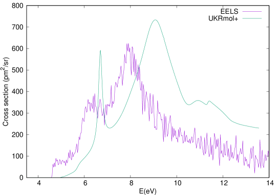
Figure 9: Cross sections for excitation into the second triplet state of thiophene for an electron scattering angle of 90^∘. The EEL spectrum was measured for an energy loss of 4.61 eV [72] and. Two core-excited resonances are clearly visible as peaks below 10 eV in both results.

This calculations was performed using MPI-SCATCI on 40 nodes (960 cores) as the Hamiltonians for each symmetry were built from around 250 000 configurations each. The option to store only the continuum coefficients was used (vecstore = 1).

8.2 Inclusion of BTOs in the continuum: electron scattering from BeH

To illustrate the capability of the codes to represent very diffuse target electronic states we show in Fig. 10 cross sections for electron scattering from BeH. The calculations and the results are described in detail in [38].

The calculations used R-matrix radius of $35\,\mbox{a${}_{0}$}$ (the largest used so far in any published molecular R-matrix calculation) and partial waves for the continuum up to $l=6$. The continuum was represented using the mixed GTO/BTO scheme as shown in Fig. 1 with the B-spline basis starting at radius $3.5\,\mbox{a${}_{0}$}$. The total number of atomic functions in the basis was $1277$. The calculation included $50$ electronic states of the target reaching up to approx. $12$ eV above the ground state: this led to construction of up to $669$ channels per symmetry in the outer region. The dimension of the inner region Hamilonians was approx. $45000$ per symmetry. In order to speed-up the outer region calculation for a fine grid of $1000$ energies we used MPI_RSOLVE, the parallel version of the RSOLVE outer region propagator: employing $60$ cores the propagation took approximately 1 hour per symmetry.

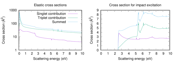
Figure 10: Cross sections for electron scattering from BeH (doublet ground state). Left panel: elastic cross sections. Right panel: cross sections for electron impact electronic excitation of the ground electronic state. No Born correction for dipolar scattering was added.

8.3 Positron scattering from H₂: use of pseudostates

A number of positron-molecule collision calculations have been performed using the UKRmol codes, e.g. [91, 92], without inclusion of a pseudocontinuum basis set and pseudostates. However, polarisation effects are even more important in positron-molecule collisions than they are in electron-molecule collisions. To address this issue, studies on positron-H₂ [5] and positron-acetylene [34] used pseudostate expansions to improve the treatment of polarisation effects which are often referred to as virtual positronium formation. These studies particularly focused on the calculation of the positron annihilation cross section as characterised by the parameter $Z_{\rm eff}$, the effective number of electrons available for positron annihilation. Use of pseudostates was found to greatly increase the computed values for $Z_{\rm eff}$, but it was found that convergence could only be achieved using pseudostate expansions which go to high $l$; in practice extrapolation formulae were used to achieve convergence.

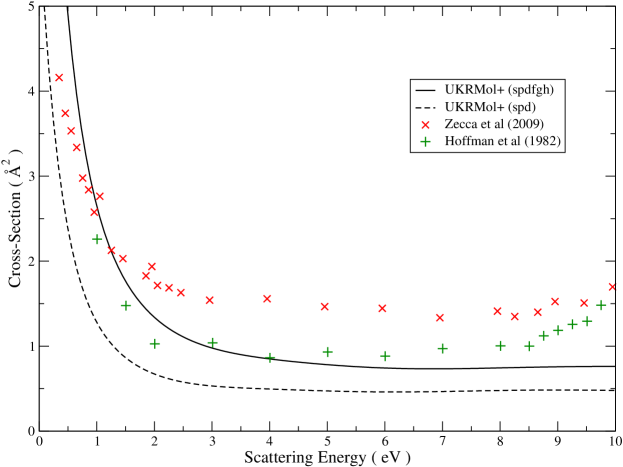
Figure 11: Total cross sections for positron-H₂ collisions. Calculations including pseudocontinuum orbitals with angular momenta up to 2 (’spd’) and up to 5 (’spdfgh’) are compared with experimental results [93, 94].

As an illustration, Figure 11 shows the total cross section for positron-H₂ calculated with the UKRmol+ suite. The models used is that of Zhang et al. [5]. The results obtained with the new suite are, as expected, similar to those of the older suite. It is also clear from the figure that increasing the number of angular momenta used for the pseudocontinuum orbitals from 3 to 6 (and also increasing the number of pseudostates from 15 to 31) improves the description of polarization effects, making the cross section larger and closer to the experimental values. The efficiency improvements implemented in the suite (in particular MPI-SCATCI) will enable both electron and positron calculations using pseudostates for larger targets: this will be particularly useful for biological molecules that tend to have big polarizabilities.

8.4 Photoionization of benzene

The recently implemented capability of the UKRmol+ suite to generate photoionization observables, Dyson orbitals and partial wave dipoles has enabled several applications, see e.g. [84, 89]. Most of these applications used high quality R-matrix data for smaller polyatomic molecules and photon energies up to $100$ eV. Nevertheless, the suite is capable of generating data for larger molecules too [86] as we demonstrate below in Fig. 12 for the case of photoionization of benzene.

These calculations were carried out using the simple HF (i.e. Static-Exchange) approximation, the cc-pVDZ atomic GTO basis set and used $20$ virtual orbitals in the $L^{2}$ expansion, see Section 2.3. The purpose of the calculations is not to present accurate observables but to illustrate the flexibility of the suite in representing the continuum and to provide an elementary guidance to the user on the current capability of the suite in representing the continuum. The size of the molecule and the wide range of photon energies typically used in experiments presents a challenge for accurate description of the continuum. Here we compare the results of calculations that used three different choices of the continuum basis:

• GTO-only continuum and integrals calculated in double precision (deletion thresholds $10^{-7}$, see Table 3).

• GTO-only continuum and integrals calculated in quad precision (deletion thresholds $10^{-14}$, i.e. no continuum orbitals removed from the basis).

• Mixed GTO/BTO continuum (double precision) with B-spline basis starting at $r=3.5$ a₀ and two choices of the parameters
  max_l_legendre_1el and max_l_legendre_2el, see Table 5.

In all cases listed above the calculations used R-matrix radius $13\,\mbox{a${}_{0}$}$ and maximum continuum angular momentum $l_{max}=6$. We have intentionally chosen a demanding example from the point of view of the size of the molecule and the corresponding mixed integral evaluation. Nevertheless, all the integral calculations presented were carried out using a single MPI task on a 20-core node equipped with 256 GB memory.

Figure 12 shows the photoionization cross sections and asymmetry parameters for the first two ionic (final) states of benzene (${}^{2}E_{1g}$ and ${}^{2}E_{2g}$). As expected the double precision GTO-only continuum performs the worst. It starts to develop unphysical oscillations in the results at approximately $25$ eV and breaks down completely at around $50$ eV. In the quad precision GTO-only continuum the basis is reliable up to approximately $50$ eV, i.e. twice that energy. However, the continuum GTO basis set used was optimized for use in scattering from a neutral target rather than in photoionization calculations and therefore the performance of this calculation could be improved employing a GTO continuum basis optimized using NUMCBAS and GTOBAS for photoionization calculations.

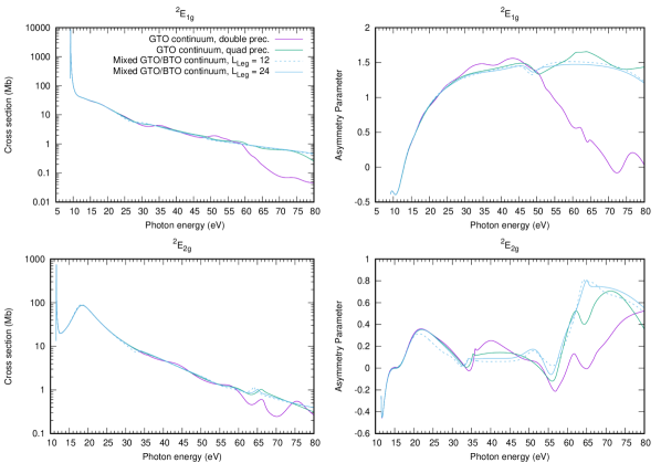
Figure 12: Cross sections (on log-scale) and $\beta$ asymmetry parameters (angular distributions) for photoionization of benzene into the two lowest-lying states (${}^{2}E_{1g}$ and ${}^{2}E_{2g}$) as calculated using GTO-only continua ($l_{max}=6$, double and quad precision) and mixed GTO/BTO continua ($l_{max}=6$ and two values of the maximum angular momentum used in the evaluation of the mixed Coulomb integrals: $L_{Leg}=12$, $L_{Leg}=24$). The ionization potentials of the final states have been shifted to their accurate values.

The quality of the mixed GTO/BTO continuum basis set is much higher, as is apparent from the asymmetry parameter for the ${}^{2}E_{1g}$ state which is smooth throughout the whole energy range, showing that the continuum basis accurately represents the highly oscillatory character of the scattering wavefunction. However, all the calculations at energies above approximately $50$ eV are not fully converged with respect to the continuum angular momentum. The figure also compares the effect of the parameters max_l_legendre_1el and max_l_legendre_2el (here denoted collectively as $L_{Leg}$) on the integral calculations in the mixed GTO/BTO basis. We can see that, as expected, with increasing electron energy the results are more sensitive to the convergence of the integrals involving continuum orbitals representing higher angular momentum electrons which in turn require higher $L_{Leg}$ to converge. In this case the minimum sensible value of these parameters ($L_{Leg}=12$) is insufficient for energies above approx. $25$ eV and a higher value ($L_{Leg}=24$) must be used to achieve more accurate results. Using higher values of $L_{Leg}$ requires more memory for evaluation of the mixed atomic integrals. Therefore convergence of the calculation with respect to this parameter should be carefully checked especially if results for high photon/electron energies are required.

Finally, the radial B-spline basis typically generates larger number of orbitals than the GTO basis with the same angular momentum. This includes continuum orbitals with near-zero amplitudes on the boundary. Therefore we can expect that the mixed continuum basis is also effectively contributing somewhat to the $L^{2}$ expansion.

9 Conclusions

The UKRmol+ suite is a completely reengineered and extended version of the UK polyatomic molecular R-matrix codes. The suite enables the calculation of low energy electron and positron (excluding positronium formation) scattering from molecules and molecular clusters, photoionization and also the production of input for the RMT suite of codes [13]. Use of the GBTOlib library (included in the releases but developed as a stand-alone entity) means that both GTOs and BTOs can be used to describe the unbound particle. The suite is maintained and developed on GitLab (developers-only access) ensuring sustainability.

The codes can be downloaded from Zenodo: provision of set of CMake files greatly simplifies the compilation of the codes; provision of a test suite enables users to test their compilation. A set of perl scripts (UKRMOL_SCRIPTS, not included in the release) is available to greatly simplify the production of input for the suite, execution of the different programs and gathering of the relevant output data. These scripts were originally developed by Dr. K. Houfek and will soon be made available for general use.

Alternatively, Quantemol-N [95] provides a graphical expert system for running the UKRmol codes; a new expert system, Quantemol-EC [96], performs the same service for the UKRmol+ codes described in this paper.

Future releases of UKRmol+ will include a new version of the GBTOlib library currently in development that will make the evaluation of the integrals more efficient, and the re-implementation of both the program for the evaluation of $Z_{\rm eff}$ in positron scattering and the partitioned R-matrix approach.

Appendix A Expressions for the boundary amplitudes

Equation (19) defines the boundary amplitudes in terms of projections of the R-matrix basis functions on the channel wavefunctions:

$$w_{pk}(a)=\frac{1}{\sqrt{2}}\bigg{\langle}\overline{\Phi}_{p}^{\Gamma}\frac{1}{r}\bigg{|}\psi_{k}^{N+1\mathrm{}}\bigg{\rangle}\bigg{|}_{r=a}=\frac{1}{\sqrt{2}}\bigg{\langle}\Phi_{p_{i}}^{N}\frac{1}{r}X_{l_{p},m_{p}}(\mathbf{r}_{N+1})\bigg{|}\psi_{k}^{N+1\mathrm{}}\bigg{\rangle}\bigg{|}_{r=a}.$$ (45)

In the UKRmol+ implementation the R-matrix basis functions are given by Eq. (21):

$$\psi_{k}^{N+1}=\hat{A}\sum_{i,j}c_{ijk}\Phi^{N}_{i}(\mathbf{x}_{1},\dots,\mathbf{x}_{N})\eta_{ij}(\mathbf{x}_{N+1})+\sum_{m}b_{mk}\chi^{N+1}_{m}(\mathbf{x}_{1},\dots,\mathbf{x}_{N+1}).$$ (46)

Using this equation and considering that only the first sum on the right-hand side contributes to the boundary amplitude we obtain:

$$w_{pk}(a) = \sum_{i,j}c_{ijk}\frac{1}{\sqrt{2}}\bigg{\langle}\overline{\Phi}_{p}^{\Gamma}\frac{1}{r}\bigg{|}\phi_{i}^{N}\eta_{ij}\bigg{\rangle}\bigg{|}_{r=a}=$$ (47)

$$= \sum_{i,j}c_{ijk}\frac{1}{\sqrt{2}}\delta_{i,p_{i}}\bigg{\langle}\frac{1}{r}X_{l_{p},m_{p}}\bigg{|}\eta_{ij}\bigg{\rangle}\bigg{|}_{r=a},$$ (48)

where we used orthonormality of the target electronic states. The matrix elements on the second line are called the raw boundary amplitudes. They are evaluated with help of expansion of the continuum orbitals $\eta_{ij}(\mathbf{x}_{N+1})$ in the single-particle basis of target, pseudocontinuum and continuum functions. However at $r=a$ only the continuum functions which have the form $f(r)X_{l,m}(\Omega)$ can contribute to the raw boundary amplitude:

$$\bigg{\langle}\frac{1}{r}X_{l_{p},m_{p}}\bigg{|}\eta_{ij}\bigg{\rangle}\bigg{|}_{r=a} = \delta_{l_{p},l_{ij}}\delta_{m_{p},m_{ij}}a\sum_{s}q_{ij,s}\gamma(a).$$ (49)

Here $q_{ij,s}$ are the coefficients in expansion of the continuum orbital $\eta_{ij}(\mathbf{x}_{N+1})$ in the basis of the single particle functions and the sum over $s$ is assumed to be only over the continuum part of the basis. The factor of $a$ is the result of the projection $\frac{1}{r}$ on the reduced radial part of the continuum orbital. Finally, $\gamma(a)$ are the amplitudes of the radial parts of the continuum functions which can be GTOs and/or BTOs (cf. Section 3.1) centered on the center of mass:

$$\gamma_{GTO,s}(a) = N_{\alpha,l_{s}}^{GTO}\sqrt{\frac{4\pi}{2l_{s}+1}}a^{l_{s}}\exp[-\alpha_{s}a^{2}],$$ (50)

$$\gamma_{BTO,s}(a) = N_{i_{s}}\frac{B_{i_{s}}(a)}{a}.$$ (51)

In UKRmol+ the raw boundary amplitudes are generated by GBTOlib at the interfacing stage, see Section 3.6.

Appendix B Irreducible representations and multiplication table

The order (and index number) of the irreducible representations in the UKRmol-in input is listed in Table 21. This mirrors the order of irreducible representations used in Molpro [9] and enables use of a single multiplication table for all groups (see Table 22). However, this convention is not universal and use of other compatible software (Psi4 [36], for instance) together with UKRmol+ requires additional attention to the ordering when writing input for SCATCI_INTEGRALS and other programs.

Table 21: Association of “$M$-values” with irreducible representations of the supported finite groups in UKRmol+.

	0	1	2	3	4	5	6	7
C1	$A$
C2	$A$	$B$
Ci	$A_{g}$	$A_{u}$
Cs	$A^{\prime}$	$A^{\prime\prime}$
C2h	$A_{g}$	$A_{u}$	$B_{u}$	$B_{g}$
C2v	$A_{1}$	$B_{1}$	$B_{2}$	$A_{2}$
D2h	$A_{g}$	$B_{3u}$	$B_{2u}$	$B_{1g}$	$B_{1u}$	$B_{2g}$	$B_{3g}$	$A_{u}$

Note that in some of the output of the calculations, for example, the target property file produced by DENPROP, the irreducible representations are numbered starting from 1.

Table 22: Multiplication table for combinations of irreducible representations of the Abelian groups supported with UKRmol+. Numbers are the $M$-values introduced in Table 21.

	0	1	2	3	4	5	6	7
0	0	1	2	3	4	5	6	7
1	1	0	3	2	5	4	7	6
2	2	3	0	1	6	7	4	5
3	3	2	1	0	7	6	5	4
4	4	5	6	7	0	1	2	3
5	5	4	7	6	1	0	3	2
6	6	7	4	5	2	3	0	1
7	7	6	5	4	3	2	1	0

Appendix C Dipole and quadrupole operators

The $(l,m)$ labeling of the matrix elements of the multipole operator produced by (C)DENPROP are subject to a convention. In UKRmol+, the electronic multipoles are written without the (negative) charge factor. When the projectile is a positron, the values receive an additional minus sign. Tab. 23 lists explicit expressions for the multipole operators used in UKRmol+.

$l$	$m$	operator	in terms of Molpro properties
1	$-1$	$y$	DMY
1	0	$z$	DMZ
1	$+1$	$x$	DMX
2	$-2$	$\sqrt{3}xy$	2 QMXY / $\sqrt{3}$
2	$-1$	$\sqrt{3}yz$	2 QMYZ / $\sqrt{3}$
2	0	$\frac{1}{2}(3z^{2}-r^{2})$	QMZZ
2	$+1$	$\sqrt{3}xz$	2 QMXZ / $\sqrt{3}$
2	$+2$	$\frac{\sqrt{3}}{2}(x^{2}-y^{2})$	(QMXX $-$ QMYY) / $\sqrt{3}$

Table 23: Multipole operators in UKRmol+ and relation to properties calculated by Molpro.

References

- [1] P. G. Burke, R-Matrix Theory of Atomic Collisions: Application to Atomic, Molecular and Optical Processes. Springer, 2011.
- [2] A. Brown et al RMT: R-matrix with time-dependence. Solving the semi-relativistic, time-dependent Schrödinger equation for general, multi-electron atoms and molecules in intense, ultrashort, arbitrarily polarized laser pulses., Computer Phys. Comm., submitted

References

- [1] P. G. Burke, K. A. Berrington (Eds.), Atomic and Molecular Processes, an R-matrix Approach, Institute of Physics Publishing, Bristol, 1993.
- [2] P. G. Burke, R-Matrix Theory of Atomic Collisions: Application to Atomic, Molecular and Optical Processes, Springer, 2011.
- [3] P. Descouvemont, D. Baye, The R-matrix theory, Rep. Prog. Phys. 73 (2010) 036301. doi:{10.1088/0034-4885/73/3/036301}.
- [4] J. Tennyson, L. K. McKemmish, T. Rivlin, Low temperature chemistry using the R-matrix method, Faraday Discuss. 195 (2016) 31–48. doi:10.1039/c6fd00110f.
- [5] R. Zhang, K. L. Baluja, J. Franz, J. Tennyson, Positron collisions with molecular hydrogen: cross sections and annihilation parameters calculated using the -matrix with pseudo-states method, J. Phys. B: At. Mol. Opt. Phys. 44 (2011) 035203.
- [6] C. J. Gillan, J. Tennyson, P. G. Burke, The UK molecular R-matrix scattering package: a computational perspective, in: W. Huo, F. A. Gianturco (Eds.), Computational methods for Electron-molecule collisions, Plenum, New York, 1995, pp. 239–254.
- [7] L. A. Morgan, C. J. Gillan, J. Tennyson, X. Chen, R-matrix calculations for polyatomic molecules: electron scattering by N2O, J. Phys. B: At. Mol. Opt. Phys. 30 (1997) 4087–4096.
- [8] J. M. Carr, P. G. Galiatsatos, J. D. Gorfinkiel, A. G. Harvey, M. A. Lysaght, D. Madden, Z. Mašín, M. Plummer, J. Tennyson, H. N. Varambhia, UKRmol: a low-energy electron- and positron-molecule scattering suite, The European Physical Journal D 66 (3) (2012) 58. doi:10.1140/epjd/e2011-20653-6.
- [9] H.-J. Werner, P. J. Knowles, G. Knizia, F. R. Manby, M. Schütz, Molpro: a general-purpose quantum chemistry program package, WIREs Comput. Mol. Sci. 2 (2012) 242–253. doi:10.1002/wcms.82.
- [10] Z. Mašín, et al, GBTOlib: library for evaluation of molecular integrals in the basis of multicentric gaussian and single-centre B-spline orbitals., Computer Physics CommunicationIn preparation.
- [11] A. G. Harvey, D. S. Brambila, F. Morales, O. Smirnova, An R-matrix approach to electron-photon-molecule collisions: photoelectron angular distributions from aligned molecules, J. Phys. B: At. Mol. Opt. Phys. 47 (2014) 215005. doi:{10.1088/0953-4075/47/21/215005}.
- [12] D. S. Brambila, A. G. Harvey, Zdeněk, J. D. Gorfinkiel, O. Smirnova, The role of multichannel effects in the photoionization of the no 2 molecule: an ab initio r -matrix study, J. Phys. B: At. Mol. Opt. Phys. 48 (2015) 245101.
- [13] A. Brown, et al., RMT: R-matrix with time-dependence. Solving the semi-relativistic, time-dependent Schrödinger equation for general, multi-electron atoms and molecules in intense, ultrashort, arbitrarily polarized laser pulses., Comput. Phys. Commun.In preparation.
- [14] P. Burke, C. Noble, V. Burke, R-matrix theory of atomic, molecular and optical processes, in: P. Berman, C. Lin, E. Arimondo (Eds.), Advances In Atomic, Molecular, and Optical Physics, Vol. 54, Academic Press, 2007, pp. 237 – 318. doi:https://doi.org/10.1016/S1049-250X(06)54005-4.
- [15] P. G. Burke, R-Matrix Theory of Atomic Collisions: Application to Atomic, Molecular and Optical Processes, Springer, 2011.
- [16] M. Gailitis, New forms of asymptotic expansions for wavefunctions of charged-particle scattering, J. Phys. B: At. Mol. Opt. Phys. 9 (1976) 843.
- [17] K. L. Baluja, P. G. Burke, L. A. Morgan, R-matrix propagation program for solving coupled second-order differential-equations, Computer Phys. Comm. 27 (1982) 299–307.
- [18] L. A. Morgan, A generalized r-matrix propagation program for solving coupled 2nd-order differential-equations, Computer Phys. Comm. 31 (1984) 419–422.
- [19] P. G. Burke, C. J. Noble, A. G. Sunderland, V. M. Burke, Electron Collisions with Iron Peak Elements: A Computational Grand Challenge, Physica Scripta T100 (2002) 55–63.
- [20] C. J. Noble, R. K. Nesbet, Cfasym, a program for the calculation of the asymptotic solutions of the coupled equations of electron collision-theory, Computer Phys. Comm. 33 (1984) 399.
- [21] R. Szmytkowski, J. Hinze, Convergence of the non-relativistic and relativistic R -matrix expansions at the reaction volume boundary, Journal of Physics B: Atomic, Molecular and Optical Physics 29 (4) (1996) 761. doi:10.1088/0953-4075/29/4/018.
- [22] H. Bachau, E. Cormier, P. Decleva, J. E. Hansen, F. Martin, Applications of b-splines in atomic and molecular physics, Rep. Prog. Phys. 64 (2001) 1815–1943.
- [23] A. Faure, J. D. Gorfinkiel, L. A. Morgan, J. Tennyson, GTOBAS: fitting continuum functions with Gaussian-type orbitals, Comp. Phys. Commun. 144 (2002) 224–241.
- [24] J. Tennyson, Electron - molecule collision calculations using the R-matrix method, Phys. Rep. 491 (2010) 29–76.
- [25] M. M. Fujimoto, W. J. Brigg, J. Tennyson, R-matrix calculations of differential and integral cross sections for low-energy electron collisions with ethanol, The European Physical Journal D 66 (2012) 204.
- [26] W. J. Brigg, J. Tennyson, M. Plummer, R-matrix calculations of low-energy electron collisions with methane, J. Phys. B: At. Mol. Opt. Phys. 47 (2014) 185203.
- [27] J. Tennyson, R-matrix calculation of Rydberg states of CO, J. Phys. B: At. Mol. Opt. Phys. 29 (1996) 6185–6201.
- [28] A. Dora, J. Tennyson, L. Bryjko, T. van Mourik, R-matrix calculation of low-energy electron collisions with uracil, J. Chem. Phys. 130 (16) (2009) 164307–8. doi:10.1063/1.3119667.
- [29] K. Bartschat, E. T. Hudson, M. P. Scott, P. G. Burke, V. M. Burke, Electron-atom scattering at low and intermediate energies using a pseudo-state R-matrix basis, J. Phys. B: At. Mol. Opt. Phys. 29 (1996) 115–123.
- [30] J. D. Gorfinkiel, J. Tennyson, Electron-H collisions at intermediate energies, J. Phys. B: At. Mol. Opt. Phys. 37 (2004) L343–L350.
- [31] J. D. Gorfinkiel, J. Tennyson, Electron impact ionisation of small molecules at intermediate energies: the R-matrix with pseudostates method, J. Phys. B: At. Mol. Opt. Phys. 38 (2005) 1607–1622.
- [32] G. Halmová, J. D. Gorfinkiel, J. Tennyson, Low and intermediate energy electron collisions with the C molecular anion, J. Phys. B: At. Mol. Opt. Phys. 41 (2008) 155201.
- [33] M. Jones, J. Tennyson, On the use of pseudostates to calculate molecular polarizabilities, J. Phys. B: At. Mol. Opt. Phys. 43 (2010) 045101.
- [34] R. Zhang, P. G. Galiatsatos, J. Tennyson, Positron collisions with acetylene calculated using the R-matrix with pseudo-states method, J. Phys. B: At. Mol. Opt. Phys. 44 (2011) 195203.
- [35] G. Schaftenaar, J. H. Noordik, Molden: a pre- and post-processing program for molecular and electronic structures, Journal of Computer-Aided Molecular Design 14 (2) (2000) 123–134. doi:10.1023/A:1008193805436.
- [36] R. M. Parrish, L. A. Burns, D. G. A. Smith, A. C. Simmonett, A. E. DePrince, E. G. Hohenstein, U. Bozkaya, A. Y. Sokolov, R. Di Remigio, R. M. Richard, J. F. Gonthier, A. M. James, H. R. McAlexander, A. Kumar, M. Saitow, X. Wang, B. P. Pritchard, P. Verma, H. F. Schaefer, K. Patkowski, R. A. King, E. F. Valeev, F. A. Evangelista, J. M. Turney, T. D. Crawford, C. D. Sherrill, Psi4 1.1: An Open-Source Electronic Structure Program Emphasizing Automation, Advanced Libraries, and Interoperability, Journal of Chemical Theory and Computation 13 (7) (2017) 3185–3197. doi:10.1021/acs.jctc.7b00174.
- [37] H. H. H. Homeier, E. O. Steinborn, Some properties of the coupling coefficients of real spherical harmonics and their relation to Gaunt coefficients, Journal of Molecular Structure: THEOCHEM 368 (1996) 31–37. doi:16/S0166-1280(96)90531-X.
- [38] D. Darby-Lewis, Z. Mašín, J. Tennyson, R-matrix calculations of electron impact electronic excitation of {BeH}, Journal of Physics B: Atomic, Molecular and Optical Physics 50 (17) (2017) 175201. doi:10.1088/1361-6455/aa8161.
- [39] A. Szabó, N. S. Ostlund, Modern quantum chemistry: introduction to advanced electronic structure theory, Courier Dover Publications, 1996.
- [40] Z. Mašín, A. G. Harvey, M. Spanner, S. Patchkovskii, M. Ivanov, O. Smirnova, Electron correlations and pre-collision in the re-collision picture of high harmonic generation, Journal of Physics B: Atomic, Molecular and Optical Physics 51 (13) (2018) 134006. doi:10.1088/1361-6455/aac598.
- [41] D. S. Brambila, A. G. Harvey, K. Houfek, Z. Mašín, O. Smirnova, Role of electronic correlations in photoionization of NO2 in the vicinity of the 2a1/2b2 conical intersection, Physical Chemistry Chemical Physics 19 (30) (2017) 19673–19682. doi:10.1039/C7CP01643C.
- [42] A. Sieradzka, J. D. Gorfinkiel, Theoretical study of resonance formation in microhydrated molecules. i. pyridine-(h2o)n, n = 1,2,3,5, The Journal of Chemical Physics 147 (3) (2017) 034302. doi:10.1063/1.4993941.
- [43] A. Sieradzka, J. D. Gorfinkiel, Theoretical study of resonance formation in microhydrated molecules. ii. thymine-(h2o)n, n = 1,2,3,5, The Journal of Chemical Physics 147 (3) (2017) 034303. doi:10.1063/1.4993946.
- [44] A. Loupas, J. D. Gorfinkiel, Shape and core-excited resonances in electron scattering from alanine, J. Chem. Phys. 150 (6) (2019) 064307. doi:10.1063/1.5081813.
- [45] J. Tennyson, A new algorithm for Hamiltonian matrix construction in electron-molecule collision calculations, J. Phys. B: At. Mol. Opt. Phys. 29 (1996) 1817–1828.
- [46] M. Yoshimine, CONSTRUCTION OF HAMILTONIAN MATRIX IN LARGE CONFIGURATION INTERACTION CALCULATIONS, J. Comput. Phys. 11 (1973) 449–454.
- [47] A. D. McLean, in: W. A. Lester Jr (Ed.), Potential Energy Surfaces in Chemistry, San Jose: IBM Research Laboratory, 1971, p. 87.
- [48] A. F. Al-Refaie, J. Tennyson, A parallel algorithm for Hamiltonian matrix construction in electron–molecule collision calculations: MPI-SCATCI, Computer Physics Communications 221 (2017) 53–62. doi:10.1016/j.cpc.2017.07.023.
- [49] A. Stathpoulos, F. C. F, A DAVIDSON PROGRAM FOR FINDING A FEW SELECTED EXTREME EIGENPAIRS OF A LARGE, SPARSE, REAL, SYMMETRICAL MATRIX, Computer Phys. Comm. 79 (1994) 268–290. doi:10.1016/0010-4655(94)90073-6.
- [50] R. Lehoucq, D. Sorensen, C. Yang, ARPACK Users’ Guide: Solution of Large-scale Eigenvalue Problems with Implicitly Restarted Arnoldi Methods, Software, Environments, Tools, Society for Industrial and Applied Mathematics, 1998.
- [51] J. Choi, J. Demmel, I. Dhillon, J. Dongarra, S. Ostrouchov, A. Petitet, K. Stanley, D. W. Walker, R. C. Whaley, ScaLAPACK: A Portable Linear Algebra Library for Distributed Memory Computers - Design Issues and Performance, in: Proceedings of the Second International Workshop on Applied Parallel Computing, Computations in Physics, Chemistry and Engineering Science, PARA ’95, Springer-Verlag, London, UK, UK, 1996, pp. 95–106.
- [52] V. Hernandez, J. E. Roman, V. Vidal, SLEPc: A scalable and flexible toolkit for the solution of eigenvalue problems, ACM Trans. Math. Software 31 (3) (2005) 351–362.
- [53] J. Tennyson, Phase factors in electron-molecule collision calculations, Computer Phys. Comm. 100 (1997) 26–30.
- [54] C. J. Gillan, J. Tennyson, B. M. McLaughlin, P. G. Burke, Low energy electron impact excitation of the nitrogen molecule: optically forbidden transitions, J. Phys. B: At. Mol. Opt. Phys. 29 (1996) 1531–1547.
-
[55]
M. Tashiro, K. Morokuma, J. Tennyson,
-matrix
calculation of electron collisions with electronically excited
molecules, Phys. Rev. A 73 (2006) 052707.
doi:10.1103/PhysRevA.73.052707.
URL https://link.aps.org/doi/10.1103/PhysRevA.73.052707 - [56] J. Tennyson, Partitioned R-matrix theory for molecules, J. Phys. B: At. Mol. Opt. Phys. 37 (2004) 1061–1071.
- [57] A. G. Harvey, D. S. Brambila, F. Morales, O. Smirnova, CDENPROP: Transition matrix elements involving continuum states, arXiv e-prints (2013) arXiv:1401.0229arXiv:1401.0229.
- [58] A. Loupas, J. D. Gorfinkiel, Shape and core-excited resonances in electron scattering from alanine, The Journal of Chemical Physics 150 (6) (2019) 064307. doi:10.1063/1.5081813.
- [59] M. Tarana, J. Tennyson, Polarization effects in electron collisions with : application of the molecular R-matrix method with pseudostates, J. Phys. B: At., Mol. Opt. Phys. 41 (2008) 205204.
- [60] I. Sukuba, J. D. Gorfinkiel, Phys. Rev. A.
- [61] Z. Mašín, J. D. Gorfinkiel, Shape and core excited resonances in electron collisions with diazines, The Journal of Chemical Physics 137 (20) (2012) 204312. doi:10.1063/1.4767345.
- [62] P. G. Burke, H. M. Schey, Elastic scattering of low-energy electrons by atomic hydrogen, Phys. Rev. 126 (1962) 147–162. doi:10.1103/PhysRev.126.147.
- [63] J. Tennyson, C. J. Noble, Reson–a program for the detection and fitting of breit-wigner resonances, Comput. Phys. Commun. 33 (1984) 421–424.
- [64] D. T. Stibbe, J. Tennyson, TIMEDEL: a program for the detection and parameterization of resonances using the time-delay matrix, Computer Phys. Comm. 114 (1-3) (1998) 236–242. doi:{10.1016/S0010-4655(98)00070-8}.
- [65] D. A. Little, J. Tennyson, M. Plummer, C. J. Noble, A. G. Sunderland, TIMEDELn: A programme for the detection and parametrization of overlapping resonances using the time-delay method, Computer Physics Communications 215 (2017) 137 – 148. doi:https://doi.org/10.1016/j.cpc.2017.01.005.
- [66] J. Tennyson, Continuum and bound states of the e- – CH+ system using the R–Matrix method, J. Phys. B: At. Mol. Opt. Phys. 21 (1988) 805–816.
- [67] N. Sanna, F. A. Gianturco, Differential cross sections for electron/positron scattering for polyatomic molecules, Computer Phys. Comm. 114 (1998) 142–167.
- [68] F. A. Gianturco, A. Jain, The theory of electron scattering from polyatomic molecules, Physics Reports 143 (6) (1986) 347–425. doi:10.1016/0370-1573(86)90125-0.
- [69] K. Regeta, M. Allan, C. Winstead, V. McKoy, Z. Mašín, J. D. Gorfinkiel, Resonance effects in elastic cross sections for electron scattering on pyrimidine: Experiment and theory, The Journal of Chemical Physics 144 (2). doi:http://dx.doi.org/10.1063/1.4937790.
- [70] R. Zhang, A. Faure, J. Tennyson, Electron and positron collisions with polar molecules: studies with the benchmark water molecule, Phys. Scripta 80 (2009) 015301.
- [71] K. Regeta, M. Allan, Z. Mašín, J. D. Gorfinkiel, Absolute cross sections for electronic excitation of pyrimidine by electron impact, The Journal of Chemical Physics 144 (2). doi:http://dx.doi.org/10.1063/1.4939077.
- [72] A. Loupas, K. Regeta, M. Allan, J. D. Gorfinkiel, Shape and core-excited resonances in thiophene, The Journal of Physical Chemistry A 122 (4) (2018) 1146–1155. doi:10.1021/acs.jpca.7b11865.
- [73] D. A. Little, J. Tennyson, Singlet and triplet ab initio Rydberg states of N2, J. Phys. B: At. Mol. Opt. Phys. 46 (2013) 145102.
- [74] B. K. Sarpal, S. E. Branchett, J. Tennyson, L. A. Morgan, Bound states using the R-matrix method: Rydberg states of HeH, J. Phys. B: At. Mol. Opt. Phys. 24 (1991) 3685–3699.
- [75] M. J. Seaton, USE OF THE R-MATRIX METHOD FOR BOUND-STATE CALCULATIONS .1. GENERAL-THEORY, J. Phys. B: At. Mol. Opt. Phys. 18 (1985) 2111–2131. doi:{10.1088/0022-3700/18/11/008}.
- [76] I. Rabadán, J. Tennyson, R-Matrix calculation of the bound and continuum states of the e- – NO+ system, J. Phys. B: At. Mol. Opt. Phys. 29 (1996) 3747–3761.
- [77] R. W. Brankin, I. Gladwell, J. R. Dormand, P. J. Prince, W. L. Seward, A RUNGE-KUTTA-NYSTROM CODE, ACM TRANSACTIONS ON MATHEMATICAL SOFTWARE 15 (1989) 31–40. doi:{10.1145/62038.69650}.
- [78] W. J. Brigg, A. G. Harvey, A. Dzarasova, S. Mohr, D. S. Brambila, F. Morales, O. Smirnova, J. Tennyson, Calculated photoionization cross sections using Quantemol-N, Jap. J. Appl. Phys. 54 (2015) 06GA02.
- [79] M. Khamesian, N. Douguet, S. F. dos Santos, O. Dulieu, M. Raoult, W. J. Brigg, V. Kokoouline, Formation of CN-, C3N-, and C5N- Molecules by Radiative Electron Attachment and their Destruction by Photodetachment, Phys. Rev. Lett. 117 (2016) 123001. doi:{10.1103/PhysRevLett.117.123001}.
- [80] D. S. Brambila, A. G. Harvey, Z. Mašín, J. D. Gorfinkiel, O. Smirnova, The role of multichannel effects in the photoionization of the NO2 molecule: An ab initio R -matrix study, J. Phys. B: At. Mol. Opt. Phys. 48 (24) (2015) 245101. doi:10.1088/0953-4075/48/24/245101.
- [81] D. S. Brambila, A. G. Harvey, K. Houfek, Z. Mašín, O. Smirnova, Role of electronic correlations in photoionization of NO2 in the vicinity of the 2A1/2B2 conical intersection, Phys Chem Chem Phys 19 (30) (2017) 19673–19682. doi:10.1039/c7cp01643c.
- [82] M. Richter, J. González-Vázquez, Z. Mašín, D. S. Brambila, A. G. Harvey, F. Morales, F. Martín, Ultrafast imaging of laser-controlled non-adiabatic dynamics in NO2 from time-resolved photoelectron emission, Phys. Chem. Chem. Phys. 21 (19) (2019) 10038–10051. doi:10.1039/C9CP00649D.
- [83] A. Rouzée, A. G. Harvey, F. Kelkensberg, D. Brambila, W. K. Siu, G. Gademann, O. Smirnova, M. J. J. Vrakking, Imaging the electronic structure of valence orbitals in the XUV ionization of aligned molecules, J. Phys. B: At. Mol. Opt. Phys. 47 (12) (2014) 124017. doi:10.1088/0953-4075/47/12/124017.
- [84] B. D. Bruner, Z. Mašín, M. Negro, F. Morales, D. Brambila, M. Devetta, D. Faccialà, A. G. Harvey, M. Ivanov, Y. Mairesse, S. Patchkovskii, V. Serbinenko, H. Soifer, S. Stagira, C. Vozzi, N. Dudovich, O. Smirnova, Multidimensional high harmonic spectroscopy of polyatomic molecules: Detecting sub-cycle laser-driven hole dynamics upon ionization in strong mid-IR laser fields, Faraday Discuss. 194 (0) (2016) 369–405. doi:10.1039/C6FD00130K.
- [85] Z. Mašín, A. G. Harvey, M. Spanner, S. Patchkovskii, M. Ivanov, O. Smirnova, Electron correlations and pre-collision in the re-collision picture of high harmonic generation, J. Phys. B: At. Mol. Opt. Phys. 51 (13) (2018) 134006. doi:10.1088/1361-6455/aac598.
- [86] D. R. Austin, F. McGrath, L. Miseikis, D. Wood, P. Hawkins, A. S. Johnson, M. Vacher, Z. Mašín, A. Harvey, M. Ivanov, O. Smirnova, J. P. Marangos, Role of tunnel ionization in high harmonic generation from substituted benzenes, Faraday Discuss. 194 (0) (2016) 349–368. doi:10.1039/C6FD00116E.
- [87] D. M. Brink, G. R. Satchler, Angular Momentum, Clarendon Press ; Oxford University Press, Oxford; New York, 1993.
- [88] B. Ritchie, Theory of the angular distribution of photoelectrons ejected from optically active molecules and molecular negative ions, Phys. Rev. A 13 (4) (1976) 1411–1415. doi:10.1103/PhysRevA.13.1411.
- [89] M. Richter, J. Gonzalez-Vazquez, Z. Mašín, D. S. Brambila, A. Harvey, F. Morales, F. Martín, Ultrafast imaging of laser-controlled non-adiabatic dynamics in NO2 from time-resolved photoelectron emission, Physical Chemistry Chemical Physicsdoi:10.1039/C9CP00649D.
- [90] I. Mayer, Simple Theorems, Proofs, and Derivations in Quantum Chemistry, US, Springer Science + Business Media New York, 2003.
- [91] K. L. Baluja, R. Zhang, J. Franz, J. Tennyson, Low-energy positron collisions with water: elastic and rotationally inelastic scattering, J. Phys. B: At. Mol. Opt. Phys. 40 (2007) 3515–3524.
- [92] A. G. Sanz, M. C. Fuss, F. Blanco, Z. Mašín, J. D. Gorfinkiel, R. P. McEachran, M. J. Brunger, G. García, Cross-section calculations for positron scattering from pyrimidine over an energy range from 0.1 to 10000 ev, Phys. Rev. A 88 (2013) 062704. doi:10.1103/PhysRevA.88.062704.
- [93] K. R. Hoffman, M. S. Dababneh, Y.-F. Hsieh, W. E. Kauppila, V. Pol, J. H. Smart, T. S. Stein, Total-cross-section measurements for positrons and electrons colliding with , , and c, Phys. Rev. A 25 (1982) 1393–1403. doi:10.1103/PhysRevA.25.1393.
- [94] A. Zecca, L. Chiari, A. Sarkar, K. L. Nixon, M. J. Brunger, Total cross sections for positron scattering from at low energies, Phys. Rev. A 80 (2009) 032702. doi:10.1103/PhysRevA.80.032702.
- [95] J. Tennyson, D. B. Brown, J. J. Munro, I. Rozum, H. N. Varambhia, N. Vinci, Quantemol-N: an expert system for performing electron molecule collision calculations using the R-matrix method, J. Phys. Conf. Ser. 86 (2007) 012001.
- [96] B. Cooper, M. Tudorovskaya, S. Mohr, A. O’Hare, M. Hanicinec, A. Dzarasova, J. Gorfinkiel, J. Benda, Z. Mašín, A. Al-Refaie, P. J. Knowles, J. Tennyson, Quantemol Electron Collision: an expert system for performing UKRmol+ electron molecule collision calculations, Atoms.