Integrable model of a $p$-wave bosonic superfluid

Abstract

We present an exactly-solvable $p$-wave pairing model for two bosonic species. The model is solvable in any spatial dimension and shares some commonalities with the $p+ip$ Richardson-Gaudin fermionic model, such as a third order quantum phase transition. However, contrary to the fermionic case, in the bosonic model the transition separates a gapless fragmented singlet pair condensate from a pair Bose superfluid, and the exact eigenstate at the quantum critical point is a pair condensate analogous to the fermionic Moore-Read state.

I Introduction

Integrable Richardson-Gaudin (RG) models Amico2001 ; Dukelsky2001 based on the $su$(2) fermion pair algebra have attracted a lot of attention in recent years. Starting with studies of the metal to superconductor transition in ultrasmall grains Duk00 , where the original Richardson’s exact solution of the BCS model Richardson1963 was rediscovered, to their generalization to a broad range of phenomena in interacting quantum many-body systems Duk04 ; Ortiz2005 . The rational or XXX family of integrable RG models has been extensively studied, and includes the constant pairing Hamiltonian (BCS model) Rich1966 ; Ortiz2005-2 ; Duk2006 , the central spin model Bortz2010 , generalized Tavis-Cummings models Duke2004 , and more recently, open quantum systems Row2018 . The hyperbolic or XXZ family is much less investigated. The notable $p+ip$ model of $p$-wave fermionic pairing Sierra2009 ; Rombouts2010 ; VanNeck2014 is an exception, having the Moore-Read (MR) Pfaffian, proposed for the non-Abelian quantum Hall fluid with filling fraction 5/2 Moo91 ; Rea00 , as ground state at a given coupling strength. Another recent finding is a number conserving version of the Kitaev wire which hosts topologically trivial and non-trivial superfluids phases Ortiz2014 . Interestingly, its repulsive version in the strong coupling limit has been shown to be related to the quantum Hall Hamiltonian projected onto the lowest Landau level subspace Ortiz2013 .

Figure 1: Quantum phase diagram of the $p$-wave bosonic Hamiltonian, Eq. (III) , in the space $g=GL$ and $\rho=N/(2L)$, where $N$ is the number of bosons and $2L$ the size of the lattice. The gray area indicates the singlet pair fragmented BEC phase, separated from the pair Bose superfluid phase (PBS) by a critical line $g_{c}$. In the superfluid phase the Volovik line, depicted by the lower dashed line, delineates the phase region where the minimum of the quasi-particle energy is at momentum $k_{\sf min}=0$, while to the right of the upper dashed line it is at $k_{\sf min}=\pi$. Between these two lines $0<k_{\sf min}<\pi$. All pairons diverge to infinity at $g_{\infty}$. Symbols indicate the couplings used below at density $\rho=0.2$. Horizontal dashed line is $\rho=0.299433$. The inset shows the behavior of the pairing gap $\Delta$ versus coupling strength $g$ at density $\rho=0.2$.

Contrary to the fermionic case, $su$(1,1) bosonic RG models are unexplored territory. Richardson introduced the bosonic constant pairing Hamiltonian Rich1967 , later generalized to study condensate fragmentation for repulsive pairing interactions Schuck2001 , and the transition from spherical to $\gamma$-unstable nuclei in the nuclear interacting boson model Pan ; Pittel . The hyperbolic $su$(1,1) RG, proposed in Dukelsky2001 , has only been employed to demonstrate the integrability of the celebrated Lipkin-Meshkov-Glick model in the Schwinger boson representation Ortiz2005 ; Pan2 ; Lerma2013 . In this Letter we derive an integrable two bosonic species $p$-wave pairing Hamiltonian, and study its quantum phase diagram. We are motivated by the recent experimental observation of broad $p$-wave resonances in ultracold ⁸⁵Rb and ⁸⁷Rb atomic mixtures Papp2008 ; Dong2016 that could lead to stable thermodynamics phases dominated by $p$-wave attractive interactions. Mean-field studies based on a two-channel model predict three phases Rad2009 : a) an atomic Bose-Einstein condensate (BEC) for large negative detuning, b) a molecular BEC for large positive detuning, and c) an atomic-molecular BEC for intermediate detuning. Quantum fluctuations may stabilize the atomic-molecular phase for certain densities giving rise to the formation of polar superfluid droplets Li2019 . Our exactly-solvable attractive one-channel $p$-wave model displays two phases (see Fig. 1), a gapless fragmented BEC of singlet pairs, where each of the species condenses into the lowest finite momentum (grey area), and a gapped pair Bose superfluid (white area).

II Hyperbolic $su$(1,1) RG integrals of motion

The hyperbolic $su$(1,1) model for two bosonic species $a$ and $b$ in momentum ${\bf k}$ space is based on the interspecies pair operators

$$K_{\mathbb{k,Q}}^{+}\!\! = \!\!b_{\mathbb{k+Q}}^{\dagger}a_{-\mathbb{k}}^{\dagger}-a_{\mathbb{k+Q}}^{\dagger}b_{-\mathbb{k}}^{\dagger},\ \ \ K_{\mathbb{k,Q}}^{-}=(K_{\mathbb{k,Q}}^{+})^{\dagger},$$ (1)

$$K_{\mathbb{k,Q}}^{z}\!\! = \!\!\frac{\hat{N}_{\mathbb{k,Q}}}{2}+1,\ \hat{N}_{\mathbb{k,Q}}=n^{b}_{\bf k+Q}+n^{b}_{\bf-k}+n^{a}_{\bf k+Q}+n^{a}_{\bf-k},$$

where $n^{b}_{\bf k}\!=b^{\dagger}_{\mathbb{k}}b^{\;}_{\mathbb{k}}$ and $n^{a}_{\bf k}\!=a^{\dagger}_{\mathbb{k}}a^{\;}_{\mathbb{k}}$. In order to satisfy the $su$(1,1) algebra $[K_{\mathbb{k,Q}}^{-},K_{\mathbb{k^{\prime},Q}}^{+}]=2\delta_{\mathbb{k},\mathbb{k^{\prime}}}K_{\mathbb{k,Q}}^{z}$ and $[K_{\mathbb{k,Q}}^{z},K_{\mathbb{k^{\prime},Q}}^{\pm}]=\pm\delta_{\mathbb{k},\mathbb{k^{\prime}}}K_{\mathbb{k,Q}}^{\pm}$, and to avoid double counting, we restrict momenta $\bf k$ and $\bf Q$ to have the component along one of the dimensions, for instance $k_{x}$, larger than zero, $k_{x}>0$ and $Q_{x}>0$. As we will see below this does not restrict the $\bf k$ values in the Brillouin zone. The operator $K_{\mathbb{k,Q}}^{+}$, that creates a two-species pair with center-of-mass momentum $\bf Q$, is antisymmetric under the exchange of species. If we interpret both species as the two components of a pseudo-spin $1/2$, the pair operator $K_{\mathbb{k,Q}}^{+}$ creates a singlet state. The pseudo-spin $1/2$ bosons define an independent and commuting $su$(2) spin algebra generated by $S_{\mathbb{k,Q}}^{z}=(n^{b}_{\bf k+Q}+n^{b}_{\bf-k}-n^{a}_{\bf k+Q}-n^{a}_{\bf-k})/2$, $S_{\mathbb{k,Q}}^{+}=b_{\mathbb{k+Q}}^{\dagger}a^{\;}_{\mathbb{k+Q}}+b_{-\mathbb{k}}^{\dagger}a^{\;}_{-\mathbb{k}}$, $S_{\mathbb{k,Q}}^{-}=(S_{\mathbb{k,Q}}^{+})^{\dagger}$. Although we will focus on the ${\bf Q}={\bf 0}$ case, these commuting algebras can be exploited to describe Larkin-Ovchinnikov-Fulde-Ferrell-type phases and/or mass imbalance two-component cold atom gases as described in Duk2006 for fermionic systems.

In terms of the $su$(1,1) generators (1), the hyperbolic integrals of motion for ${\bf Q}={\bf 0}$ are Dukelsky2001 ; Ortiz2005

$$R_{\mathbb{k}} = K_{\mathbb{k}}^{z}-2\lambda\sum_{\mathbb{k}^{\prime}(\not=\mathbb{k})>0}\left[\frac{\eta_{\mathbb{k}}\eta_{\mathbb{k}^{\prime}}}{\eta_{\mathbb{k}}^{2}-\eta_{\mathbb{k^{\prime}}}^{2}}\left(K_{\mathbb{k}}^{+}K_{\mathbb{k}^{\prime}}^{-}+K_{\mathbb{k}}^{-}K_{\mathbb{k}^{\prime}}^{+}\right)\right.$$ (2)

$$\left.-\frac{\eta_{\mathbb{k}}^{2}+\eta_{\mathbb{k}^{\prime}}^{2}}{\eta_{\mathbb{k}}^{2}-\eta_{\mathbb{k}^{\prime}}^{2}}K_{\mathbb{k}}^{z}K_{\mathbb{k}^{\prime}}^{z}\right],$$

where $\eta_{\mathbb{k}}$ are arbitrary odd functions of ${\bf k}$. The sum $\mathbb{k}^{\prime}>0$ means that the component $k^{\prime}_{x}$ should be positive.

For a fixed number of bosons $N=2M+\nu$, where $M$ is the number of singlet boson pairs and $\nu$ the total number of unpaired bosons, the eigenvalues of the integrals of motion are

$$r_{\mathbb{k}}=d_{\mathbb{k}}\left[1+2\lambda\sum_{\mathbb{k}^{\prime}(\not=\mathbb{k})>0}d_{\mathbb{k}^{\prime}}\frac{\eta_{\mathbb{k}}^{2}+\eta_{\mathbb{k}^{\prime}}^{2}}{\eta_{\mathbb{k}}^{2}-\eta_{\mathbb{k}^{\prime}}^{2}}-2\lambda\sum_{\alpha=1}^{M}\frac{e_{\alpha}+\eta_{\mathbb{k}}^{2}}{e_{\alpha}-\eta_{\mathbb{k}}^{2}}\right],$$

where $d_{\mathbb{k}}=\nu_{\mathbb{k}}/2+1$, $\nu_{\mathbb{k}}$ is the seniority quantum number (number of unpaired bosons) of level $\mathbb{k}$, and $\nu=\sum_{\mathbb{k}>0}\nu_{\mathbb{k}}$. The spectral parameters $e_{\alpha}$, so-called pairons, are roots of the Richardson equations $(\alpha=1,\dots,M)$

$$\sum_{\mathbb{k}>0}\frac{d_{\mathbb{k}}}{\eta_{\mathbb{k}}^{2}-e_{\alpha}}+\sum_{\beta=1(\beta\not=\alpha)}^{M}\frac{1}{e_{\beta}-e_{\alpha}}+\frac{\tilde{Q}}{e_{\alpha}}=0,$$ (3)

with

$$\tilde{Q}=-\frac{1}{4\lambda}+\frac{M-1+\sum_{\mathbb{k}>0}d_{\mathbb{k}}}{2}.$$

Each independent solution of the Richardson equations (3) defines a common eigenstate of the integrals of motion (2):

$$|\Phi_{M,\nu}\rangle=\prod_{\alpha=1}^{M}\left(\sum_{\mathbb{k}>0}\frac{\eta_{\mathbb{k}}}{\eta_{\mathbb{k}}^{2}-e_{\alpha}}K_{\mathbb{k}}^{+}\right)|\nu\rangle,$$ (4)

where the state $|\nu\rangle$, with $\nu$ unpaired bosons, satisfies $\hat{K}_{\mathbb{k}}^{-}|\nu\rangle=0$ for all $\mathbb{k}$, and $\hat{K}_{\mathbb{k}}^{z}|\nu\rangle=d_{\mathbb{k}}|\nu\rangle$.

By combining the integrals of motion $R_{\bf k}$ with the Hellmann-Feynman theorem Rombouts2010 , the occupation probabilities can be obtained from the expectation value

$$\left\langle\Phi_{M,\nu}|K_{\mathbf{k}}^{z}|\Phi_{M,\nu}\right\rangle=d_{\mathbf{k}}\left(1-2\lambda^{2}\sum_{\alpha=1}^{M}\frac{2\eta_{\mathbf{k}}^{2}}{\left(\eta_{\mathbf{k}}^{2}-e_{\alpha}\right)}\frac{\partial e_{\alpha}}{\partial\lambda}\right),$$ (5)

where the pairon derivatives can be obtained from the derivatives of Eq. (3) leading to a linear set of equations. For ease of presentation we consider next a one-dimensional version of the $p$-wave model. It is straightforward to extend our model to higher dimensions as has been done in the fermionic case Sierra2009 ; Rombouts2010 .

III The $p$-wave Bose Hamiltonian

The $p$-wave pairing Bose Hamiltonian we want to study is given by

$$H = \sum_{k}\eta_{k}^{2}\left(a^{\dagger}_{k}a^{\;}_{k}+b_{k}^{\dagger}b^{\;}_{k}\right)$$

$$-\frac{G}{4}\sum_{k,k^{\prime}}\eta_{k}\eta_{k^{\prime}}\left(b_{k}^{\dagger}a_{-k}^{\dagger}-a_{k}^{\dagger}b_{-k}^{\dagger}\right)\text{\Large$($}b^{\;}_{k^{\prime}}a^{\;}_{-k^{\prime}}-a^{\;}_{k^{\prime}}b^{\;}_{-k^{\prime}}\text{\Large$)$}$$

where $\eta_{k}=\sin(k/2)$ and $\eta_{k}^{2}=(1-\cos k)/2$. Assuming antiperiodic boundary conditions the allowed $k$ values are $k=\pm\pi/2L,\pm 3\pi/2L,\dots,\pm(2\pi L-\pi)/2L$, with $2L$ the size of the chain and $L$ the number of $su$(1,1) copies. We have chosen antiperiodic boundary conditions to explicitly exclude the $k=0$ state. This state cannot support singlet pairs and, therefore, it will be excluded from the dynamics of $p$-wave pair scattering. This model Hamiltonian, which written in terms of the $su(1,1)$ generators is

$$H=\sum_{k>0}\eta_{k}^{2}\,\hat{N}_{k}-G\sum_{k,k^{\prime}>0}\eta_{k}\eta_{k^{\prime}}K_{k}^{+}K_{k^{\prime}}^{-},\\$$ (7)

can be derived from the hyperbolic $su$(1,1) RG integrals of motion (2), by using the linear combination

$$H=2x\sum_{k>0}\eta_{k}^{2}R_{k}-2Z-G\sum_{k>0}d_{k}(1-d_{k})\eta_{k}^{2},$$

where $x=[1+2\lambda(M+L+(\nu/2)-1)]^{-1}$, $Z=\sum_{k>0}\eta_{k}^{2}$, and $G=4\lambda/(1+2\lambda(M-1+\sum_{k>0}d_{k}))$.

Our $p$-wave Hamiltonian (7) has an explicit U(1) symmetry, i.e., conservation of the total number of bosons, and a pseudospin invariance that basically preserves the polarization $S^{z}=\sum_{k}S^{z}_{k}$, that is, the difference between the number of bosonic species. Here we will focus on an unpolarized mixture of atoms characterized by $S^{z}=0$, although the polarized case ($S^{z}\neq 0$) is contained in our exact solution. For instance, an excess of $a$ atoms manifests through the seniorities $\nu_{k}$ specifying the $k$ states occupied by the unpaired $a$ atoms.

Eigenvalues of (7) can be determined from the integrals of motion, using the same linear combination, which, after using Eq. (3), gives

$$E=\sum_{k>0}\eta_{k}^{2}\nu_{k}+2\sum_{\alpha=1}^{M}e_{\alpha}.$$ (8)

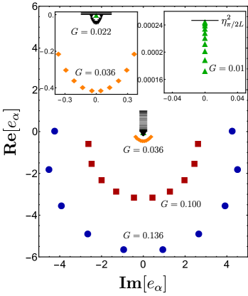
Figure 2: Pairons, $e_{\alpha}$, for a finite system with $M=10$ pairs and $L=50$ levels ($\rho=M/L=0.2$). Cases displayed correspond to the five symbols indicated in Fig. 1. Coupling strengths $G$ are indicated by numbers close to the respective symbols. Horizontal lines depict $\eta_{k}^{2}$ levels. See SM for an animation of the pairons evolution as a function of $G$ for $0<G<G_{\infty}$.

Let us analyze next the way the ground state evolves as a function of coupling strength $G\geq 0$ (Fig. 2). Each independent solution of the Richardson equations (3) provides a set of $M$ pairons that define both the energy eigenvalue (8) and the corresponding eigenstate (4). The ground state (with $\nu=0$) for weak coupling $G$ has the pairons distributed in the real interval between zero and the minimum $\eta_{\pi/2L}^{2}=\sin^{2}(\pi/4L)$. At $G_{n}=2/(2L+2M-n-1)$, $n$ pairons collapse to zero. In between collapses, the $n$ pairons expand as complex conjugate pairs forming an arc in the complex plane around zero. The whole set of $M$ pairons collapses to zero at the critical point

$$G_{c}=\frac{2}{2L+M-1},$$

where the exact (non-normalized) ground state becomes a condensate of singlet pairs

$$\left|\Phi_{M}\right\rangle_{\sf BMR}=\left(\sum_{k>0}\frac{1}{\eta_{k}}K_{k}^{+}\right)^{M}\left|0\right\rangle,$$ (9)

which is algebraically analogous to the MR state of the $p+ip$ fermionic model Sierra2009 ; Rombouts2010 , and, therefore, we will call it Bose Moore-Read (BMR) state.

Naively, in an extended system, one would expect that the ground state of the BEC phase, $0\leq G\leq G_{c}$, corresponds to a zero-momentum condensate for each species

$$\left|\Phi\right\rangle=a_{0}^{\dagger M}b_{0}^{\dagger M}\left|0\right\rangle$$ (10)

since, as we will see, the quasi-particle gap $\Delta$ vanishes. This state has maximum spin $S=M$. For mesoscopic systems, it has been shown that the correct ground state at weak coupling is a fragmented singlet pair BEC Kuklow ; Leggett , which in momentum space becomes

$$\left|\Phi\right\rangle=(K^{+}_{k_{\sf min}})^{M}\!\!\left|0\right\rangle=\left(b_{k_{\sf min}}^{\dagger}a_{-k_{\sf min}}^{\dagger}-a_{k_{\sf min}}^{\dagger}b_{-k_{\sf min}}^{\dagger}\right)^{M}\!\!\left|0\right\rangle,$$ (11)

with $k_{\sf min}=\pi/2L$ for the antiperiodic chain. Note that in this phase, the exact ground state has a mixture of complex pairons close to zero and real pairons in the interval $[0,\eta^{2}_{\pi/2L}]$. For large $L$ the pairons will cluster around zero and the exact ground state (4) will tend to the BMR state (9) which is representative of the whole phase. The BMR state is controlled by $k_{\sf min}$, and therefore it converges to the singlet pair condensate in the large $L$ limit. Interestingly, in the thermodynamic limit the states (11) and (10), as well as condensates with other spin quantum numbers $S$, become degenerate. A weak repulsive interaction may destabilize those degenerate spin states against the singlet pair condensate Leggett .

For $G>G_{c}$ the pairons distribute along an arc that expands in the complex plane as $G$ increases (Fig. 2). At

$$G_{\infty}=\frac{2}{M-1}$$

the absolute value of all pairons diverges to infinity. This divergence does not affect the energy since imaginary parts cancel out pairwise in (8) and the real parts combine to give $E=2GM\sum_{k>0}\eta^{2}_{k}$. Infinite pairon energies have been observed previously in fermionic hyperbolic models Ortiz2014 and they were related to a duality associated to the particle-hole symmetry Links . At this point the exact ground state can be expressed as a different pair condensate

$$|\Phi_{M}\rangle_{G_{\infty}}=\left(\sum_{k}\eta_{k}\,K_{k}^{+}\right)^{M}|0\rangle.$$ (12)

In turn, in the fermionic case we find that this state appears as the highest energy eigenstate in the repulsive pairing region.

In Fig. 1, at density $\rho=0.2$, we show five distinct symbols covering all distinct areas of the phase diagram, at couplings $g=0.5,1.2,1.8,5.0,6.8$, with $g=GL$. Figure 2 displays pairons of a finite-sized system with $M=10$ and $L=50$, for these same five values. As discussed above, the first point with $G<G_{c}$ has 10 pairons distributed in the real positive axis below $\eta^{2}_{\pi/2L}$ (see the right inset). After the pairons collapse to zero at $G_{c}$, they form an arc in the complex plane that expands for increasing values of $G$. This is the case for the remaining four couplings that lay in between $G_{c}$ and $G_{\infty}$, two of them can be seen in the left inset while the other two in the central figure.

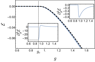
Figure 3: Energy density ${\cal E}$ as a function of $g$. Continuous lines are the thermodynamic limit solution while the dashed line is the exact ${\cal E}$ for $M=10$ and $L=50$. Second and third-order derivatives of $\cal E$ are displayed in the insets.

IV Quantum Phase Diagram

The thermodynamic limit is obtained in the limit of $N,L\rightarrow\infty$ with constant density $\rho=N/(2L)$ and rescaled interaction strength $g=GL$. In this limit, the Richardson equations (3) transform into the boson gap and number equations Rombouts2010 ; Ortiz2005-2

$$\frac{\pi}{g}=\int_{0}^{\pi}\frac{\eta_{k}^{2}}{E_{k}}\,dk,\;\;\ \ \ \ \rho=\frac{2}{\pi}\int_{0}^{\pi}v_{k}^{2}\,dk,$$ (13)

with quasi-boson energies $E_{k}$ and occupation probabilities $v_{k}^{2}$

$$E_{k}=\sqrt{\left({\eta_{k}^{2}}-\mu\right)^{2}-4\eta^{2}_{k}\Delta^{2}},\;\;v^{2}_{k}=\frac{1}{2}\left(\frac{\eta_{k}^{2}-\mu}{E_{k}}-1\right),$$ (14)

where $\mu$ is the chemical potential and $\Delta$ the gap. Though $E_{k}$ in (14) may, in principle, be complex, we have numerically verified that in the large attractive $g$ limit, Eqs. (13) have solutions $\mu\approx-\gamma_{1}g$ and $\Delta\approx\gamma_{2}g$, with $\gamma_{1,2}$ positive constants satisfying $4\gamma_{2}^{2}<\gamma_{1}^{2}$. This latter condition guarantees that the quasi-boson energies, given by $E_{k}\approx g\gamma_{1}\sqrt{1-(4\gamma_{2}^{2}/\gamma_{1}^{2})\eta_{k}^{2}}$ are always real, even in the limit $g\rightarrow\infty$. The ground state energy density ${\cal E}\equiv E/L$ for a given density $\rho$ in the thermodynamic limit is given by

$${\cal E}=-\frac{4\Delta^{2}}{g}-1+\frac{2}{\pi}\int_{0}^{\pi}\frac{\eta_{k}^{2}(\eta_{k}^{2}-\mu)}{E_{k}}\,dk.$$ (15)

The critical coupling of the exact solution in the finite-size case, becomes $g_{c}=\lim_{L,N\rightarrow\infty}[G_{c}L]=2/(2+\rho)$ in the thermodynamic limit. The gap $\Delta$ is zero at weak pairing up to the critical value $g_{c}$. The inset of Fig. 1 shows the behavior of the gap for $\rho=0.2$. It increases monotonically for $g>g_{c}$. In the same thermodynamic limit, the coupling where all pairons diverge becomes $g_{\infty}=\lim_{L,N\rightarrow\infty}[G_{\infty}L]=2/\rho$ (Fig. 1).

We are interested in establishing the nature of the non-analyticities of ${\cal E}$ at the critical point. It turns out that ${\cal E}=0$, for $0<g<g_{c}$ and is non-analytic at $g=g_{c}$ with a third order phase transition to a pair superfluid phase Rombouts2010 ; Lerma2011 . Close to $g-g_{c}\approx 0^{+}$, it behaves as

$${\cal E}\approx-\frac{\pi^{2}}{3}\left(\frac{\tilde{g}}{g}\right)^{2}\left(\frac{\tilde{g}}{g}-12\frac{g-1}{ge^{2(2-g_{c})}}\ e^{\frac{2(g_{c}-1)}{\tilde{g}}}\right),$$ (16)

where $\tilde{g}=(g-g_{c})/g_{c}$ (See Appendix A). Interestingly, the behavior of $\cal E$ close to $g_{c}$ depends on $\rho$ only through its critical value $g_{c}$. The first and second-order derivatives at the critical point are zero, while the third-order derivative is $\partial_{g}^{3}{\cal E}\rfloor_{g-g_{c}\rightarrow 0^{+}}=-2\pi^{2}/g_{c}^{6}$, signaling a discontinuity of third order. This is illustrated in Fig. 3 for $\rho=0.2$ where, moreover, ${\cal E}$ is compared with the exact energy density for $M=10$ and $L=50$.

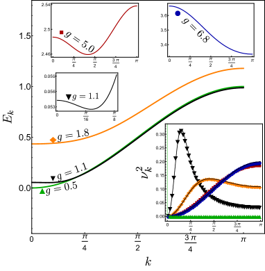
Figure 4: Quasi-particle energies for $\rho=0.2$ and the same couplings as those indicated in Fig. 1. For $g=1.1$, the inset zooms in the low-$k$ region, showing that $k_{\sf min}\not=0$. Lower inset displays the occupation probabilities.

V Nature of excitations

In Fig. 4 we show the quasi-boson energies for the five values of $g$ indicated in Fig. 1. The quasi-boson energies change from $E_{k}=\sin^{2}(k/2)$ in the gapless pair condensate phase ($g=0.5$), to a complex dispersion in the pair Bose superfluid phase. For $\mu+2\Delta^{2}\leq 0$, $E_{k}$ is a monotonous increasing function with minimum at $k_{\sf min}=0$ and energy $E_{k_{\sf min}}=|\mu|$ ($g=1.8$). The previous condition is fulfilled in the superfluid phase only for small densities $\rho<0.299433$ in a finite coupling interval. The region is indicated by the area with diagonal lines in Fig. 1. The boundary of this region, the so called Volovik line Sierra2009 defined by a superfluid with the minimum quasi-boson energy at $k=0$, is given by $\mu+2\Delta^{2}=0$. For $0<\mu+2\Delta^{2}<1$, $E_{k}$ has a minimum at $k_{\sf min}=2\arcsin(\sqrt{\mu+2\Delta^{2}})$, satisfying $0<k_{\sf min}<\pi$ ($g=1.1,5.0$). The region of the phase diagram where $E_{k}$ has this dispersion is indicated by the white area in Fig. 1. The previous condition is fulfilled for any density, and gives the form of the quasi-boson dispersion immediately after the quantum phase transition. For $\mu+2\Delta^{2}\geq 1$ (area with horizontal lines in Fig. 1), the quasi-boson dispersion is a monotonous decreasing function with minimum at $k_{\sf min}=\pi$ ($g=6.8$).

The occupation probabilities in momentum space are displayed in the lower inset of Fig. 4 for the five values of $g$ indicated in Fig. 1. Continuous lines are the thermodynamic limit solution and symbols correspond to the exact solution for the finite-size case calculated using Eq. (5). For $g=0.5$ the system is condensed in $k_{\sf min}$ resulting in a delta distribution in the thermodynamic limit. At $g_{c}$, in that limit, the macroscopic occupation at $k_{\sf min}\rightarrow 0$ jumps to zero and then the maximum of the distribution moves to finite $k$ values. This jump in the $k=0$ momentum state resembles the one observed in the $p+ip$ and RG Kitaev models Rombouts2010 ; Ortiz2014 and the $s$-$d$ RG model of Ref. Claeys2018 . In the fermionic case, this fact has been linked to a topological phase transition Rombouts2010 ; Ortiz2014 . For $g=1.1$ and $1.8$ the profiles broaden and maxima get displaced to larger values of $k$. Finally, for $g=5.0$ and $6.8$ the profiles are inverted with a maximum occupation at $k=\pi$.

VI Outlook

We introduced an exactly-solvable two species $p$-wave bosonic model and established its quantum phase diagram in the attractive sector. Only the case of a balanced mixture with equal masses ($m_{a}=m_{b}$) and zero center-of-mass momentum ${\bf Q}$ has been studied in depth. Imbalanced binary mixtures ($\nu\neq 0$, $m_{a}\neq m_{b}$) and finite ${\bf Q}$ pairs are contained within our exactly solvable model. The exact, finite and thermodynamic limit, treatments of the $p$-wave pairing Bose Hamiltonian (7), although seemingly similar, have profound physical differences to its fermionic counterpart Sierra2009 ; Rombouts2010 ; VanNeck2014 ; Links despite the fact that both cases share a third-order quantum phase transition. In the fermionic case the latter separates two gapped superfluid phases and has a topological character Ortiz2014 . In the bosonic case one of the phases is gapless and displays a fragmented BEC condensate with macroscopic occupations of both species in the lowest finite momentum pair states $(-k,k)$, while the other is a gapped pair Bose superfluid (PBS). Moreover, while for fermions the critical coupling takes place at the Read-Green point, with one pairon at zero energy and the other $M-1$ pairons with real and negative energies, for bosons the phase transition takes place at the equivalent of the fermionic Moore-Read point with all pairons collapsing to zero energy. It is at this critical point that the exact bosonic ground state is a pair condensate with amplitudes fixed by the single particle energies.

Motivated by a theoretical prediction Petrov , recent experiments unveiled a new type of ultradilute quantum liquid in ultracold bosonic systems. Apparently, there is no unique mechanism leading to such a liquid state since it has been observed in single-species dipolar systems Kadau and Bose (potassium) mixtures Semeghini ; Cabrera . Can one obtain a quantum liquid phase in $p$-wave Bose systems? This question has been recently addressed in Li2019 , and answered in the affirmative for a particular model. Our PBS represent a (fixed-point) number-conserving candidate for such quantum liquid phase. The pairing interaction in (7) may thus provide a new effective mechanism for its emergence. Although the superfluid gap protects that state from expansion in finite geometries, further studies in trapped potentials are required to identify a possible self-bound quantum liquid droplet. On the experimental side, it is crucial to have a precise understanding of the spectrum of excitations to compare to our theoretical predictions.

Acknowledgments— S.L.-H. acknowledges financial support from the Mexican CONACyT project CB2015-01/255702. J.D. is supported by the Spanish Ministerio de Ciencia, Innovación y Universidades, and the European regional development fund (FEDER) under Projects No. FIS2015-63770-P and PGC2018-094180-B-I00, S.L.-H. and J.D. acknowledges financial support .from the Spanish collaboration Grant I-COOP2017 Ref:COOPB20289. G.O acknowledges support from the US Department of Energy grant DE-SC0020343.

Appendix A Non-analytic behavior at the quantum critical point

One can write the boson gap and number equations (13), in the thermodynamic limit, as

$$\pi(\rho+1) = \int_{0}^{1}dx\frac{x-\mu}{\sqrt{x-x^{2}}\sqrt{x^{2}-2ax+\mu^{2}}}$$ (17)

$$\frac{\pi}{g} = \int_{0}^{1}dx\frac{x}{\sqrt{x-x^{2}}\sqrt{x^{2}-2ax+\mu^{2}}},$$ (18)

where the following change of variables has been performed: $x=\eta_{k}^{2}$, and $a=\mu+2\Delta^{2}$.

We are interested in characterizing the behavior of physical quantities, such as the chemical potential $\mu$, superfluid gap $\Delta$, and ground state energy density $\cal E$, near the phase transition $g\approx g_{c}$ where a non-analyticity develops. Close to the transition, and for couplings $g>g_{c}$, $\mu<0$ and $a>0$, such that $a>\delta=\mu^{2}-a^{2}>0$. We need to determine the behavior of the above integrals in the limit $\delta\rightarrow 0^{+}$. A few algebraic steps lead to:

$$\int_{0}^{1}dx\frac{1}{\sqrt{x-x^{2}}\sqrt{x^{2}-2ax+\mu^{2}}}\stackrel{{\scriptstyle\delta\rightarrow 0^{+}}}{{=}}I_{d}$$

$$I_{d}=\sqrt{\frac{1}{a-a^{2}}}\left(\log 16+2\log(a-a^{2})-\log\delta\right).$$ (19)

Similar manipulations result in

$$\int_{0}^{1}dx\frac{x-a}{\sqrt{x-x^{2}}\sqrt{x^{2}-2ax+\mu^{2}}} \stackrel{{\scriptstyle\delta\rightarrow 0^{+}}}{{=}} \pi-4\arcsin\sqrt{a}.$$

Therefore, the resulting gap and number equations close to the critical point become

$$\pi\rho = -4\arcsin\sqrt{a}+(a-\mu)\,I_{d}$$ (20)

$$\frac{\pi}{g} = \pi-4\arcsin\sqrt{a}+a\,I_{d},$$ (21)

or equivalently

$$\rho+1 = \frac{1}{g}-\frac{\mu}{a}\left(\frac{1}{g}-1+\frac{4}{\pi}\arcsin\sqrt{a}\right),$$ (22)

and whose consistency can be checked by taking the limit $a\rightarrow 0$, $g\rightarrow g_{c}$. This gives $\rho+1=2/g_{c}$, as expected from the exact solution. On the other hand, we would like to determine the behavior of the gap $\Delta$ and chemical potential $\mu$ as a function of $\rho$ and $g$ close to the transition. It turns out to be more convenient to write $a-\Delta^{2}=\mu+\Delta^{2}=\mu\,\Gamma$, and find solutions for $\mu$ and $\Gamma$

$$\mu \approx -\left(\frac{\pi}{2}\right)^{2}\left(\frac{g-g_{c}}{g\,g_{c}}\right)^{2}$$ (23)

$$\Gamma \approx 4\,e^{2(g_{c}-2)}e^{\frac{2g_{c}(g_{c}-1)}{g-g_{c}}},$$ (24)

What is the behavior of the ground state energy density $\cal E$, Eq. (15),

$${\cal E} = -\frac{4\Delta^{2}}{g}-1+\frac{2}{\pi}\int_{0}^{1}dx\frac{x(x-\mu)}{\sqrt{x-x^{2}}\sqrt{x^{2}-2ax+\mu^{2}}}$$

close to the phase transition? Following the same strategy, close to the transition point,

$$\int_{0}^{1}\!\!dx\frac{x(x-\mu)}{\sqrt{x-x^{2}}\sqrt{x^{2}-2ax+\mu^{2}}}\stackrel{{\scriptstyle\delta\rightarrow 0^{+}}}{{=}}\frac{\pi}{2}\left[2(a(\rho+1)-\mu)\right.$$

$$\left.+1\right]+2\left(\sqrt{a(1-a)}+(2\mu-1)\arcsin\sqrt{a}\right),$$

and to first order in powers of $\Gamma$, it results

$${\cal E}\approx-\frac{\pi^{2}}{3}\left(\frac{\tilde{g}}{g}\right)^{2}\left(\frac{\tilde{g}}{g}-12\frac{g-1}{ge^{2(2-g_{c})}}\ e^{\frac{2(g_{c}-1)}{\tilde{g}}}\right),$$ (25)

where $\tilde{g}=(g-g_{c})/g_{c}$, displaying a discontinuity of third order as indicated in the main text.

References

• (1) L. Amico, A. Di Lorenzo, and A. Osterloh, Phys. Rev. Lett. 86, 5759 (2001).
• (2) J. Dukelsky, C. Esebbag, and P. Schuck, Phys. Rev. Lett. 87, 066403 (2001).
• (3) G. Sierra, J. Dukelsky, G. G. Dussel, J. von Delft, and F. Braun, Phys. Rev. B 61, R11890 (2000).
• (4) R. W. Richardson, Phys. Lett. 3, 277 (1963).
• (5) J. Dukelsky, S. Pittel, and G. Sierra, Rev. Mod. Phys. 76, 643 (2004).
• (6) G. Ortiz, R. Somma, J. Dukelsky, and S. M. A. Rombouts, Nucl. Phys. B 707, 421 (2005).
• (7) R. W. Richardson, Phys. Rev. 141, 949 (1966).
• (8) G. Ortiz and J. Dukelsky, Phys. Rev. A 72, 043611 (2005).
• (9) J. Dukelsky, G. Ortiz, S. M. A. Rombouts, and K. Van Houcke, Phys. Rev. Lett. 96, 180404 (2006).
• (10) M. Bortz, S. Eggert, and J. Stolze, Phys. Rev. B 81, 035315 (2010).
• (11) J. Dukelsky, G. G. Dussel, C. Esebbag, and S. Pittel, Phys. Rev. Lett. 93, 050403 (2004).
• (12) D. A. Rowlands, and A. Lamacraft, Phys. Rev. Lett. 120, 090401 (2018).
• (13) M. I. IbaΓ±ez, J. Links, G. Sierra, and S. Y. Zhao, Phys. Rev. B 79, 180501(R) (2009).
• (14) S. M. A. Rombouts, J. Dukelsky, and G. Ortiz, Phys. Rev. B 82, 224510 (2010).
• (15) G. Ortiz, J. Dukelsky, E. Cobanera, C. Esebbag, and C. Beenakker, Phys. Rev. Lett. 113, 267002 (2014).
• (16) J. Links, I. Marquette, and A. Moghaddam, J. Phys. A: Math. Theor. 48 (2015) 374001.
• (17) M. Van Raemdonck, S. De Baerdemacker, and D. Van Neck, Phys. Rev. B 89, 155136 (2014).
• (18) G. Moore and N. Read, Nucl. Phys. B 360, 362 (1991).
• (19) N. Read and D. Green, Phys. Rev. B 61, 10267 (2000).
• (20) G. Ortiz, Z. Nussinov, J. Dukelsky, and A. Seidel, Phys. Rev. B 88, 165303 (2013).
• (21) R. W. Richardson, J. Math. Phys. 9, 1327 (1967).
• (22) J. Dukelsky and P. Schuck, Phys. Rev. Lett. 86, 4207 (2001).
• (23) F. Pan and J. P. Draayer, Nucl. Phys. A 636, 156 (1998).
• (24) J. Dukelsky and S. Pittel, Phys. Rev. Lett. 86, 4791 (2001).
• (25) F. Pan and J. P. Draayer, Phys. Lett. B 451, 1 (1999).
• (26) S. Lerma H. and J. Dukelsky, Nucl. Phys. B 870, 421 (2013).
• (27) S. Papp, J. Pino, and C. Wieman, Phys. Rev. Lett. 101, 040402 (2008).
• (28) S. Dong, Y. Cui, C. Shen, Y. Wu, M. K. Tey, L. You, and B. Gao, Phys. Rev. A 94, 062702 (2016).
• (29) L. Radzihovsky and S. Choi, Phys. Rev. Lett. 103, 095302 (2009).
• (30) Z. Li, J.-S. Pan, and W. Vincent Liu, arXiv:1905.08463.
• (31) See Supplemental Material at [URL will be inserted by publisher] for an animation of the pairons evolution as a function of coupling strength.
• (32) A. B. Kuklov and B.V. Svistunov, Phys. Rev. Lett. 89, 170403 (2002).
• (33) S. Ashhab and A. J. Leggett, Phys. Rev. A 68, 063612 (2003).
• (34) S. Lerma H., S. M. A. Rombouts, J. Dukelsky, and G. Ortiz, Phys. Rev. B 84, 100503(R) (2011).
• (35) E. Stouten, P. W. Claeys, J.-S. Caux, and V. Gritsev, Phys. Rev. B 99, 075111 (2019).
• (36) D. S. Petrov, Phys. Rev. Lett. 115, 155302 (2015).
• (37) H. Kadau et. al., Nature 530, 194 (2016).
• (38) G. Semeghini et. al., Phys. Rev. Lett. 120, 235301 (2018).
• (39) C. R. Cabrera et. al., Science 359, 301 (2018).