Short Non-Binary Low-Density Parity-Check Codes for Phase Noise Channels

Abstract

This work considers the design of short non-binary low-density parity-check (LDPC) codes over finite fields of order $m$, for channels with phase noise. In particular, $m$-ary differential phase-shift keying (DPSK) modulated code symbols are transmitted over an additive white Gaussian noise (AWGN) channel with Wiener phase noise. At the receiver side, non-coherent detection takes place, with the help of a multi-symbol detection algorithm, followed by a non-binary decoding step. Both the detector and decoder operate on a joint factor graph. As a benchmark, finite length bounds and information rate expressions are computed and compared with the codeword error rate (CER) performance, as well as the iterative threshold of the obtained codes. As a result, performance within $1.2$ dB from finite-length bounds is obtained, down to a CER of $10^{-3}$.

I Introduction

In the context of the upcoming fifth generation (5G) standard for cellular communications, massive machine-type communications (mMTC) are considered to be one of the key applications [1], [2]. In this scenario, small devices, for instance sensors, sparsely transmit small amounts of data. To keep the cost of such devices small, low-end oscillators might be used, which give rise to phase noise. Furthermore, non-binary modulation schemes might be employed, in order to efficiently exploit the available spectrum. Also, the number of pilots for estimating the channel is chosen such that the overall transmission overhead is kept as small as possible, while maintaining sufficient quality of the channel estimate [3].

Whenever short frames are considered, e.g., in the order of a few hundred symbols, pilots may yield a non-negligible loss in spectral efficiency. A remedy consists in dropping the usage of pilots and using a differential modulation scheme, such as DPSK, with non-coherent detection at the receiver [4, 5, 6]. To recover the performance gap with respect to the coherent case, i.e., when full phase information is available at the receiver, non-coherent detectors, which use multiple symbols to compute a decision, may be used in practice. For sufficiently long sequences, they are shown to perform close to coherent schemes [4], [7].

Depending on various constraints, two approaches can be taken to reliably communicate in this scenario [6]. In the first approach, differential modulation can be used together with a standard forward error correcting code [8]. This results in a serial turbo scheme that is then decoded by iteratively exchanging soft information between the detector and decoder. This has been previously used on a variety of channels [9, 8, 5]. Alternatively, the channel code itself may be modified and made resilient to phase uncertainties, as demonstrated, e.g., in [10, 11].

Code design for phase noise channels has been widely addressed in the literature. In [6, 12] the authors investigate different detection algorithms to counteract phase noise. The detector is concatenated with the decoder of various binary codes from the literature to form a turbo detection scheme. Binary LDPC code design for continuous phase frequency shift keying modulation and a blockwise non-coherent AWGN channel was performed in [13] for a bit-interleaved coded modulation scheme. In [14], a code design for binary codes using differential modulation was considered. It was shown that taking into account the differential modulator in the code design yields performance gains. The work in [15] extends [12], by introducing an accumulator based LDPC code design. Iterative decoding thresholds for irregular ensembles are provided, while finite-length designs were not investigated. In [16], a similar scheme for multiple-input and multiple-output communications was presented, where the detector was merged with the check node (CN) decoder of a binary repeat accumulate code.

Initial work on non-binary convolutional codes over rings, using phase-shift keying (PSK) modulation, dates back to [17, 18], where various convolutional code designs were presented for the AWGN channel. In order to make the codes robust against block-wise phase noise, an additional differential modulator is suggested in [18], without yet considering powerful turbo detection at the receiver.

A binary LDPC code design for binary phase shift keying (BPSK) and Wiener phase noise, with turbo and blind phase estimation, was presented in [19]. During code construction, some local CNs are introduced to resolve phase ambiguities. In [10], the work is extended to quaternary phase shift keying (QPSK) using $4$-ary codes over rings. The scheme is shown to handle Wiener phase noise with a standard deviation of up to $2^{\circ}$. In both cases, codewords of a few thousand bits are considered. LDPC codes over rings for PSK modulation and the coherent AWGN channel were studied in [20].

In [21], a surrogate non-binary LDPC code design over a finite field for the AWGN channel was presented. The codes were adapted to the non-coherent phase noise channel and showed excellent performance for short blocks. This work is a continuation of [21], where we further elaborate on the code design.

In the following, we focus on transmission of short blocks over AWGN channels with Wiener phase noise. To achieve reliable communication, we make use of a coded modulation system, where a non-binary LDPC code over a field of order $m$ is interfaced with a DPSK scheme of order $m$ through a symbol interleaver. At the receiver, detection and decoding are performed on a joint factor graph, making use of the discretized-phase (DP) algorithm for the detector [12] and the non-binary belief propagation (BP) algorithm [22] for the LDPC code decoder.

This contribution differs from the literature, as the focus is on short blocks (in the order of a few hundred symbols) with application to mMTC. In contrast to many existing works, we make use of non-binary LDPC codes over finite fields, owing to their excellent performance over the AWGN channel for short blocks [22, 23, 24, 25]. Compared to [21], we directly perform the code design of the concatenated scheme for the non-coherent Wiener phase noise channel and also present useful finite-length benchmarks for this channel. Furthermore, we introduce a refinement step in the code design process, aiming at lowering the error-floor.

The paper is organized as follows. Section II provides some background on the notation used, the channel model and the receiver structure. In Section III the performance bounds used to benchmark our results are presented, followed by Section IV where the code design is described. Finally, in Section V some numerical results are provided and are followed by Section VI where some conclusions are drawn.

II System Setup

II-A Transmitter Description

Throughout this paper, we will consider a coded modulation system as depicted in Figure 1. Here, a length-$K$ information frame $\mathbf{u}=(u_{1},u_{2},\ldots,u_{K})$, is encoded by a non-binary code $\mathcal{C}$ over the finite field of order $m$, $\mathbb{F}_{m}$. This yields a length-$N$ codeword $\mathbf{v}=(v_{1},v_{2},\ldots,v_{N})$. Both $\mathbf{u}$ and $\mathbf{v}$ are non-binary vectors whose elements belong to $\mathbb{F}_{m}$.

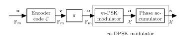
Figure 1: Transmitter block diagram.

The symbols of the codeword vector $\mathbf{v}$ are then interleaved by means of a (random) interleaver $\pi$, yielding $\mathbf{c}=(c_{1},c_{2},\ldots,c_{N})$, and input to an $m$-ary DPSK modulator, where the field and modulation order are matched to each other. Differential modulation is performed in two steps. At first the non-binary symbols $c_{i}$, are mapped to complex constellation points belonging to $\mathcal{X}=\left\{e^{j2\pi l/m}\right\}$, $l\in\{0,\ldots,m-1\}$. This results in $N$ complex modulation symbols, $\mathbf{a}=(a_{1},a_{2},\ldots,a_{N})$, $a_{i}=e^{j\varphi_{i}}$. In the second step, the phase of these symbols is accumulated, obtaining the transmitted symbols $\mathbf{s}=(s_{0},s_{1},\ldots,s_{N})$. By expressing $\phi_{i}=\arg(s_{i})$, the phase accumulator implements $\phi_{i}=[\phi_{i-1}+\varphi_{i}]_{2\pi}$, where $[\cdot]_{2\pi}$ denotes the operation modulo $2\pi$, and outputs $N+1$ symbols, with $s_{0}=1$.

In the following, we will always assume that the non-binary code order is matched to the modulation order and that $m>2$. We also denote by $k$ and $n$ the number of information and codeword bits in $\mathbf{u}$ and $\mathbf{v}$ respectively, with $k=K\log_{2}m$, $n=N\log_{2}m$. We define the code rate of the code $\mathcal{C}$ as $R_{C}=K/N=k/n$.

II-B Channel Model

The DPSK symbols $s_{i}$ are transmitted over an AWGN channel affected by phase noise. To model the phase noise, we make use of a popular model from literature [6], i.e., the Wiener model. Hence, the received sample $r_{i}$ is given by

$$r_{i} =s_{i}e^{j\theta_{i}}+n_{i}$$ (1)

$$=e^{j\phi_{i}}e^{j\theta_{i}}+n_{i}$$

$$=e^{j\psi_{i}}+n_{i}$$ (2)

where $\theta_{i}$ is an unknown phase rotation introduced by the channel and $n_{i}$ are independent AWGN samples distributed as

$$n_{i}\sim\mathcal{CN}\left(0,2\sigma^{2}\right).$$

According to the Wiener model we have that

$$\theta_{i}=\theta_{i-1}+\Delta\theta_{i}$$ (3)

where $\Delta\theta_{i}$ are independent, distributed as

$$\Delta\theta_{i}\sim\mathcal{N}\left(0,\sigma_{\Delta}^{2}\right)$$

with $\theta_{0}$ uniformly distributed in $[0,2\pi)$. The phase of the received signal $\psi_{i}$ is obtained as $\psi_{i}=[\theta_{i}+\phi_{i}]_{2\pi}$.

As a reference, we also evaluate the performance of our system on a coherent AWGN channel, obtained by setting $\theta_{i}=0,\forall i$ in (1).

II-C Iterative Detection and Decoding at the Receiver

The block diagram in Figure 2 illustrates the exchange of messages at the receiver. First, the detector processes the received samples $\mathbf{r}$ together with the a priori information $\mathbf{L}^{\mathsf{A},\mathsf{det}}$ on the modulated codeword sequence $\mathbf{a}$, available from the decoder. The message vector $\mathbf{L}^{\mathsf{A},\mathsf{det}}=(\mathbf{L}_{1}^{\mathsf{A},\mathsf{det}},\mathbf{L}_{2}^{\mathsf{A},\mathsf{det}},\ldots,\mathbf{L}_{N}^{\mathsf{A},\mathsf{det}})$ is a vector of $N$ probability mass functions, having $m$-dimensional components $\mathbf{L}_{i}^{\mathsf{A},\mathsf{det}}$. The same holds for all the other vectors, $\mathbf{L}^{\mathsf{E},\mathsf{det}}$, $\mathbf{L}^{\mathsf{A},\mathsf{dec}}$, $\mathbf{L}^{\mathsf{E},\mathsf{dec}}$, $\mathbf{L}^{\mathsf{APP},\mathsf{dec}}$.

We have that $\mathbf{L}_{i}^{\mathsf{A},\mathsf{det}}=\mathbf{P}(a_{i})$ is initially set to $[1/m,\ldots,1/m]$. The detector computes soft extrinsic information $\mathbf{L}^{\mathsf{E},\mathsf{det}}$ on the modulated codeword symbols $\mathbf{a}$ with $\mathbf{L}_{i}^{\mathsf{E},\mathsf{det}}=k\mathbf{P}(a_{i}|\mathbf{r})/\mathbf{P}(a_{i})$, with the division performed element-wise and followed by a normalization step (denoted as such by multiplication with constant $k$). The elements of $\mathbf{L}^{\mathsf{E},\mathsf{det}}$ are de-interleaved and provided as a priori information on the code symbols $\mathbf{v}$ to the decoder. Second, from these a priori messages, the decoder computes a posteriori messages $\mathbf{L}^{\mathsf{APP},\mathsf{dec}}$, with $\mathbf{L}_{i}^{\mathsf{APP},\mathsf{dec}}\approx\mathbf{P}(v_{i}|\mathbf{L}_{i}^{\mathsf{A},\mathsf{dec}})$ and extrinsic messages $\mathbf{L}^{\mathsf{E},\mathsf{dec}}$, with $\mathbf{L}_{i}^{\mathsf{E},\mathsf{dec}}={k}\mathbf{L}_{i}^{\mathsf{APP},\mathsf{dec}}/\mathbf{L}_{i}^{\mathsf{A},\mathsf{dec}}$, where again the division is performed element wise and is followed by a normalization step. The extrinsic messages are interleaved and provided to the detector as a priori information, which can be used to compute refined estimates of $\mathbf{L}_{i}^{\mathsf{E},\mathsf{det}}$. The message exchange between the decoder and detector is iterated for a certain number of times, before a decision on the code symbols, based on $\mathbf{L}^{\mathsf{APP},\mathsf{dec}}$, is made.

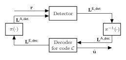
Figure 2: Block diagram of the iterative receiver.

In the following, we describe the structure of the detector based on the work in [12], [21], followed by a discussion on the decoder.

II-C1 Detection

The role of the detector is to provide an estimate of the symbol-wise probability $\mathbf{P}(a_{i}|\mathbf{r})$, which is divided element-wise by the priors $\mathbf{P}(a_{i})$ and normalized, to obtain the extrinsic information $\mathbf{L}_{i}^{\mathsf{E},\mathsf{det}}$ that is forwarded to the decoder. It is computed starting with the factorization [6]

$$\begin{split}p(\mathbf{a},\boldsymbol{\psi}|\mathbf{r})&=p(\mathbf{r}|\mathbf{a},\boldsymbol{\psi})p(\boldsymbol{\psi}|\mathbf{a})P(\mathbf{a})\frac{1}{p(\mathbf{r})}\\ &\propto p(r_{0}|\psi_{0})\prod_{i=1}^{N}p(r_{i}|\psi_{i})p(\psi_{i}|\psi_{i-1},a_{i})P(a_{i})\,\end{split}$$ (4)

where due to the Wiener model and the differential modulation $p(\psi_{i}|\psi_{i-1},\ldots,\psi_{0},\mathbf{a})=p(\psi_{i}|\psi_{i-1},a_{i})$. This factorization allows us to make use of factor graphs [26] and compute $P(a_{i}|\mathbf{r})/P(a_{i})$ as

$$\frac{P(a_{i}|\mathbf{r})}{P(a_{i})}=\int\displaylimits_{{0}}^{{2\pi}}\int\displaylimits_{{0}}^{{2\pi}}\alpha(\psi_{i-1})\beta(\psi_{i})p(\psi_{i}|\psi_{i-1},a_{i})d\psi_{i}d\psi_{i-1}$$ (5)

where $\alpha(\psi_{i})$ and $\beta(\psi_{i})$ equal [12]

$$\begin{split}\alpha(\psi_{i})&=p(r_{i}|\psi_{i})\int\displaylimits_{0}^{2\pi}\left(\sum_{a_{i}}p(\psi_{i}|\psi_{i-1},a_{i})P(a_{i})\right)\alpha(\psi_{i-1})\ d\psi_{i-1}\end{split}$$ (6)

$$\begin{split}\beta&(\psi_{i})=p(r_{i}|\psi_{i})\int\displaylimits_{0}^{2\pi}\left(\sum_{a_{i+1}}p(\psi_{i+1}|,\psi_{i},a_{i+1})P(a_{i+1})\right)\beta(\psi_{i+1})\ d\psi_{i+1}\end{split}$$ (7)

with $\alpha(\psi_{0})=p(r_{0}|\psi_{0})$ and $\beta(\psi_{N})=p(r_{N}|\psi_{N})$.

To compute $\alpha(\psi_{i})$ and $\beta(\psi_{i})$, we proceed as follows. Firstly, $p(r_{i}|\psi_{i})$ is a complex Gaussian probability density function (p.d.f.) with mean $e^{j\psi_{i}}$ and variance $\sigma^{2}$ per dimension. For the coherent case, where there is no phase uncertainty, i.e., $\theta_{i}=0,\forall i$, in the above iterations, the probability $p(\psi_{i}|\psi_{i-1},a_{i})$ reduces to an indicator function

$$p(\psi_{i}|\psi_{i-1},a_{i})\overset{\theta_{i}=0}{=}\mathbbm{1}(e^{j\phi_{i}}=a_{i}e^{j\phi_{i-1}})=\begin{cases}1,&\text{if}\ e^{j\phi_{i}}=a_{i}e^{j\phi_{i-1}}\\ 0,&\text{otherwise}\end{cases}.$$ (8)

The detector implements nothing else but the Bahl Cocke Jelinek Raviv (BCJR)[27] algorithm on the trellis of the differential modulator.

For the non-coherent case we start with the Wiener model in (3) and the identity $\phi_{i}=[\phi_{i-1}+\varphi_{i}]_{2\pi}$, which allows us to write $\psi_{i}=[\psi_{i-1}+\varphi_{i}+\Delta\theta_{i}]_{2\pi}$. Since $a_{i}=e^{j\varphi_{i}}$ is a deterministic mapping between $\varphi_{i}$ and $a_{i}$, it holds that

$$p(\psi_{i}|\psi_{i-1},a_{i})=p(\psi_{i}|\psi_{i-1},\varphi_{i})=p_{\Delta}(\psi_{i}-\psi_{i-1}-\varphi_{i})$$ (9)

where $p_{\Delta}(\cdot)$ is the p.d.f. of the phase-noise increment $\Delta\theta_{i}$ (modulo $2\pi$). For brevity we denote $x=\Delta\theta_{i}$ and hence

$$p_{\Delta}(x)=\sum\displaylimits_{\ell=-\infty}^{+\infty}g(0,\sigma_{\Delta}^{2};x-2\pi\ell)$$ (10)

where

$$g(\mu,\sigma_{\Delta}^{2};x)=\frac{1}{\sqrt{2\pi\sigma_{\Delta}^{2}}}e^{-\frac{(x-\mu)^{2}}{2\sigma_{\Delta}^{2}}}\,$$ (11)

since the increment $\Delta\theta_{i}$ is normally distributed.

For the values that $\sigma_{\Delta}$ takes in practice, the p.d.f. in (11) is approximately zero in all points, except for some points in the vicinity of $\mu$ [15]. Hence, we can approximate

$$p_{\Delta}(x)\simeq g(0,\sigma_{\Delta}^{2};x)$$ (12)

and simplify (10) to

$$p_{\Delta}(\psi_{i}-\psi_{i-1}-\varphi_{i})\simeq g(0,\sigma_{\Delta}^{2};\psi_{i}-\psi_{i-1}-\varphi_{i})\,.$$ (13)

Still, using (13) in (5), (6) and (7), the computations are rather complex, since they involve evaluating integrals of continuous p.d.f.s. A possible solution to this problem is to discretize the channel phase and implement the so-called DP algorithm [6]. We hence assume that $\psi_{i}$ is discrete and belongs to the set $\{2\pi j/L\}$, $j\in\{0,\ldots,L-1\}$, with $L$ being the number of discretization levels. Moreover, [8] suggests using a further simplification

$$p_{\Delta}(x)=\begin{cases}1-P_{\Delta},&x=0\\ \frac{P_{\Delta}}{2},&|x|=\frac{2\pi}{L}\\ 0,&\text{else}\end{cases}$$ (14)

with $P_{\Delta}$ being an optimization parameter obtained via simulation. For all our simulations we have used $P_{\Delta}=0.1$. It has been shown that a phase discretization factor of $L=8m$ is enough to obtain negligible losses with respect to the unquantized case. With these two approximations, the integrals in (5), (6) and (7) become summations and the computation of all values above becomes feasible in practice.

II-C2 Decoding

The code $\mathcal{C}$ is assumed to be an LDPC code. Thus, standard belief propagation for non-binary LDPC codes from the literature can be applied. For more details on non-binary decoding of LDPC codes, the reader is referred, e.g., to [22], [28]. For our setup, we perform only one iteration of the belief propagation algorithm within the decoder at a time, and allow a maximum of $N_{\mathrm{it}}=200$ iterations between the detector and decoder. This value was chosen in accordance with the literature on non-binary LDPC codes (see, e.g., [22, 24, 29, 30]).

III Performance Bounds

We use two benchmarks to assess the performance of our system. The first one is the information rate, which gives a lower bound on the achievable rate when the block length goes to infinity. It is defined as

$$\lim\limits_{N\rightarrow\infty}\frac{1}{N}\mathbb{E}\left[{\log_{2}\frac{p(\mathbf{R}|\mathbf{S})}{p(\mathbf{R})}}\right]=\lim\limits_{N\rightarrow\infty}\frac{1}{N}\mathbb{E}\left[{i(\mathbf{S};\mathbf{R})}\right]$$ (15)

where $i(\cdot;\cdot)$ denotes the information density and $\mathbf{S}$ and $\mathbf{R}$ are random vectors associated to the process describing the transmitted and received symbols, respectively. To compute it, we resort to the methods of [31] as described in [15].

As a finite-length performance benchmark we compute the dependency testing (DT) bound [32], which provides an upper bound to the average block error probability $P_{B}$ of a random code with $M=m^{K}$ codewords of length $N+1$. Following [32] we obtain

$${P_{B}} {\leq\mathbb{E}\left[{2^{-\Big{(}i(\mathbf{S};\mathbf{R})-\log_{2}\frac{M-1}{2}\Big{)}^{+}}}\right]}$$ (16)

$${\approx\frac{1}{D}\sum_{(\mathbf{s},\mathbf{r})}{2^{-\Big{(}i(\mathbf{s};\mathbf{r})-(K\log_{2}m-1)\Big{)}^{+}}}}$$ (17)

where $(x)^{+}\equiv\max(x,0)$ and $D$ is the number of $(\mathbf{s},\mathbf{r})$ tuples. Analogously to the computation of the information rate, we compute the information density as described in [32], following a Monte Carlo approach. To this end, we randomly generate an input sequence of DPSK modulated symbols $\mathbf{s}$, which we transmit over the communication channel to obtain $\mathbf{r}$. For the tuple $(\mathbf{s},\mathbf{r})$ we then evaluate the information density $i(\mathbf{s};\mathbf{r})$ and the corresponding summand in (17). We repeat this experiment $D$ times and average over the outcomes. For the communication channel used to compute $\mathbf{r}$, we either use a Wiener phase noise channel, as defined in (2) or a coherent AWGN channel, both yielding different expressions for the information density in (17).

IV Code Design

We are interested in the design of $m$-ary LDPC codes for $m$-DPSK modulation over a non-coherent Wiener phase noise channel, described in Section II. Our methodology for the code design is as follows. First, we aim to find a protograph LDPC code ensemble with an iterative decoding threshold close to the theoretically achievable limit. In an optional second step, we refine the protograph code design, aiming at error floors below a target block error probability. Next, a brief introduction on protograph LDPC codes is given, followed by a discussion on the computation of the iterative decoding threshold. Then, a detailed description of the protograph search algorithm is provided. The section is complemented by some remarks on the algorithm.

IV-A Protograph LDPC Codes

Protograph-based binary LDPC codes were originally introduced in [33]. This class of structured LDPC codes performs excellently on a wide class of communication channels while the code structure permits hardware friendly implementations. A protograph can be any Tanner graph, typically one with a relatively small number of nodes [33] which are connected by single or multiple edges. In the protograph, each variable node (VN) and CN is said to be of a certain type. The protograph can be seen as a template for the bipartite graph of an LDPC code, which is obtained by lifting the protograph through “copy-and-permute” operations. For this, $\ell$ copies of the protograph are generated and interconnected as follows. Edges among all copies are permuted such that if a node of type $i$ was connected to a node of type $j$ in the protograph, then any of its $\ell$ copies are connected to any of the $\ell$ copies of the node of type $j$. After expansion, parallel edges are no longer permitted. In order to optimize the girth of the resulting graph, we perform the expansion by a circulant version of the progressive edge growth (PEG) algorithm [34]. A protograph can be represented by a $m_{b}\times n_{b}$ base matrix $\mathbf{B}$ whose entries $b_{ij}$ give the number of edges connecting a CN of type $i$ to a VN of type $j$. Note that a protograph, or alternatively its base matrix, describe an ensemble of LDPC codes.

Non-binary protographs were first introduced in [24], and can be divided into constrained and unconstrained protographs [35]. The former ones possess additional edge labels from $\mathbb{F}_{m}\backslash\{0\}$. After expansion, these labels correspond to the non-binary coefficients in the code’s parity-check matrix. In this work, our attention is on unconstrained protographs, for which no edge labels are assigned at protograph level. Rather, the edge labels are assigned after the final expansion step and are chosen uniformly at random from $\mathbb{F}_{m}\backslash\{0\}$.

IV-B Iterative Decoding Threshold Computation

The iterative decoding threshold of an LDPC code ensemble is defined as the worst channel parameter for which the ensemble average probability of symbol error vanishes, when the block length and the number of decoding iterations go to infinity. Iterative decoding thresholds of unstructured non-binary LDPC code ensembles for AWGN channels can be conveniently computed by making use of extrinsic information transfer (EXIT) analysis [36]. The extension to non-binary protograph ensembles can be done by adapting the results in [37].

We have computed iterative decoding thresholds for protograph LDPC code ensembles over $\mathbb{F}_{m}$ adopting Method 1 from [36]. Here, the log-probability ratios, passed on the edges of the bipartite graph, are approximated as multivariate Gaussian random variables. We have found empirically that the computed thresholds obtained by Method 1 provide limited accuracy for the setup in Figure 1. To increase the accuracy of the threshold computation, the authors in [36] propose Method 2. This method can be adapted to non-binary protograph LDPC codes and requires measuring the transfer function, for each VN and CN type in the protograph, which relates the extrinsic mutual information at the output of a node to the a priori mutual information at its input. Measuring the transfer function imposes a high computational burden, in particular if various protographs are tested, each with different node types. In this case, EXIT analysis loses its advantage of providing a low-complexity alternative to other techniques, such as Monte Carlo density evolution [38].

We therefore resort to Monte Carlo density evolution [38] to obtain the thresholds. In brief, the iterative decoding threshold of a protograph LDPC code ensemble is obtained by performing decoding on a large bipartite graph, where iteration by iteration, the edge interleavers between the different node types are changed in order to emulate the average ensemble behavior (see [38, 39] for details). We also make use of channel adapters for the iterative decoding threshold computation and resort to the all-zero codeword assumption [36]. Note that, owing to the protograph structure of the LDPC codes, we place an interleaver between the detector and decoder, similarly to [40]. For the threshold computation we use a different random interleaver for every decoding attempt. The computational cost of Monte Carlo density evolution is still too high to enable the use of iterative optimization algorithms, such as differential evolution [41], for the search of protographs with good iterative decoding thresholds. For this reason, we propose a simplified protograph search methodology, aiming to reduce the protograph search space.

IV-C Protograph Search

On the coherent AWGN channel, let us denote the input constrained Shannon limit in terms of energy per information bit to noise power spectral density ratio by $\left(E_{b}/N_{0}\right)_{\mathsf{c}}^{\mathsf{Sh}}$ and the iterative decoding threshold of a protograph LDPC code ensemble by $\left(E_{b}/N_{0}\right)_{\mathsf{c}}^{*}$. Similarly, on the non-coherent Wiener phase noise channel the theoretical limit from the information rate expression in Section III is named $\left(E_{b}/N_{0}\right)_{\mathsf{nc}}^{\mathsf{Sh}}$, while the iterative decoding threshold of a protograph ensemble is termed $\left(E_{b}/N_{0}\right)_{\mathsf{nc}}^{*}$. Also, we denote by $\mathbb{Z}_{p}$ the set of non-negative integers smaller than $p$. We introduce the following definitions.

Definition 1.

An $m_{b}\times n_{b}$ single entry matrix $\mathbf{Q}$ is a matrix whose entry $q_{i,j}=1$ for some $i,j$ and all other entries are set to zero.

Definition 2.

A minimal set $\mathcal{M}_{e}$ of $m_{b}\times n_{b}$ matrices is a set for which an element $\mathbf{B}\in\mathcal{M}_{e}$ cannot be obtained by row and/or column permutation of any other element in $\mathcal{M}_{e}$.

Minimal sets are of particular interest, since the iterative decoding threshold of a protograph does not change by permuting the rows and/or columns of the associated base matrix. Hence, in the following, we start from a set $\mathcal{M}$ of protograph base matrices and generate a minimal set $\mathcal{M}_{e}$ out of it, as follows. We start with an empty set $\mathcal{M}_{e}$ and pick one element of $\mathcal{M}$ after the other. We include an element of $\mathcal{M}$ in $\mathcal{M}_{e}$, if, after inclusion, $\mathcal{M}_{e}$ is still a minimal set. Otherwise, the element is rejected. We formalize the protograph search algorithm as follows.

First Step (Threshold Optimization)

Our objective is to find a protograph with iterative decoding threshold $\left(E_{b}/N_{0}\right)_{\mathsf{nc}}^{*}$ on the Wiener phase noise channel as close as possible to $\left(E_{b}/N_{0}\right)_{\mathsf{nc}}^{\mathsf{Sh}}$. We consider only a small number of protographs for which iterative decoding thresholds are computed and proceed as follows.

First, generate all $p^{m_{b}n_{b}}$ $m_{b}\times n_{b}$ base matrices whose elements $b_{i,j}$ are picked from $\mathbb{Z}_{p}$ yielding the set $\mathcal{M}$. Expurgate $\mathcal{M}$ by imposing constraints on the base matrices contained in it: discard an element if it contains zero weight columns or if the number of weight-$1$ columns exceeds $m_{b}$. Generate a minimal set $\mathcal{M}_{e}$ out of the expurgated set and compute iterative decoding thresholds for the elements of $\mathcal{M}_{e}$. Select the base matrix $\mathbf{B}_{\text{}}^{*}$ with the best iterative decoding threshold and expand it to obtain an $(N,K)$ LDPC code as discussed in Section IV-A. Finally, evaluate the code performance on the Wiener phase noise channel by Monte Carlo simulation.

Second Step (Refinement)

If the simulation results show a visible error floor above a target block error probability, we attempt to lower the error floor by changing the code design as follows.

The base matrix $\mathbf{B}_{\text{}}^{*}$ from step 1) is expanded by a factor of $\ell^{\prime}$, where ${\ell^{\prime}}=\max_{i,j}b^{*}_{i,j}$ is the largest base matrix entry. The expansion is done according to the description in Section IV-A. This yields the $m_{b}^{\prime}\times n_{b}^{\prime}$ base matrix $\mathbf{B}_{\text{}}^{\prime}$, with $m_{b}^{\prime}={\ell^{\prime}}m_{b}$. Generate a new set ${\mathcal{M}}^{\prime}$ where each element is obtained by adding to $\mathbf{B}_{\text{}}^{\prime}$ a different $m_{b}^{\prime}\times n_{b}^{\prime}$ single entry matrix. This yields a set with cardinality $|{\mathcal{M}}^{\prime}|=m_{b}^{\prime}n_{b}^{\prime}$, since there are $m_{b}^{\prime}n_{b}^{\prime}$ distinct $m_{b}^{\prime}\times n_{b}^{\prime}$ single entry matrices. Note that the matrices in ${\mathcal{M}}^{\prime}$ have an increased average column and row weight with respect to $\mathbf{B}_{\text{}}^{*}$, which is expected to improve the distance properties of the corresponding ensemble and hence to lower the error floor (see, e.g., [42, 43]). Next, a minimal set ${\mathcal{M}}^{\prime}_{e}$ is generated out of ${\mathcal{M}}^{\prime}$. Iterative decoding thresholds for the base matrices in ${\mathcal{M}}^{\prime}_{e}$ are computed and the one with the best iterative decoding threshold is selected. By expansion, an $(N,K)$ LDPC code is obtained and simulated on the Wiener phase noise channel. In the case that the error floor is no longer visible above the target block error probability the algorithm stops, otherwise step 2 is repeated by selecting the next best candidate in ${\mathcal{M}}_{e}$.

IV-D Remarks

We conclude the section with the following remarks. Firstly, for a given code rate, the dimensions $m_{b}$ and $n_{b}$ of the base matrix are picked to be as small as possible in order to limit the search space. For instance, for code rates $R=(r-1)/r$, base matrices of size $1\times r$ are considered. Secondly, the base matrix entries $b_{i,j}$ are chosen from $\mathbb{Z}_{4}$. This is motivated by the fact that non-binary LDPC codes with VN degrees of three and less show excellent performance on Gaussian channels [25, 23].

V Numerical Results

In the following, we present some code design examples by applying the rule described in Section IV. We also provide theoretical benchmarks based on the results in Section III. In particular, for the coherent AWGN case, the Shannon limit $\left(E_{b}/N_{0}\right)_{\mathsf{c}}^{\mathsf{Sh}}$ and DT bound are computed. For the non-coherent case, the respective theoretical limit $\left(E_{b}/N_{0}\right)_{\mathsf{nc}}^{\mathsf{Sh}}$ and DT bound are given. Different DPSK orders (thus field orders), code rates and standard deviations of the phase noise increment are considered. In particular, the standard deviation of the phase noise increment is $\sigma_{\Delta}=2^{\circ}$ for 8-PSK and $\sigma_{\Delta}=1^{\circ}$ for 16-PSK. The mapping between field elements and $8$-PSK, as well as $16$-PSK symbols, are provided in Tables I and II, respectively. A target block error probability of $10^{-3}$ is assumed, above which no visible error floor should occur. This falls in the range of error probabilities currently discussed for mMTC in 5G.

TABLE I: Mapping between $\mathbb{F}_{8}$ code symbols, their binary image, and Gray labeled $8$-PSK modulation symbols. The primitive polynomial for $\mathbb{F}_{8}$ is $1+\mathrm{x}+\mathrm{x}^{3}$.

$\mathbb{F}_{8}$ element	Binary label	$8$-PSK symbol
$0$	$000$	$1$
$\alpha^{0}$	$001$	$e^{j\pi/4}$
$\alpha^{1}$	$010$	$e^{j3\pi/4}$
$\alpha^{2}$	$100$	$e^{j7\pi/4}$
$\alpha^{3}$	$011$	$e^{j\pi/2}$
$\alpha^{4}$	$110$	$e^{j\pi}$
$\alpha^{5}$	$111$	$e^{j5\pi/4}$
$\alpha^{6}$	$101$	$e^{j3\pi/2}$

TABLE II: Mapping between $\mathbb{F}_{16}$ code symbols, their binary image, and Gray labeled $16$-PSK modulation symbols. The primitive polynomial for $\mathbb{F}_{16}$ is $1+\mathrm{x}+\mathrm{x}^{4}$.

$\mathbb{F}_{16}$ element	Binary label	$16$-PSK symbol
$0$	$0000$	$1$
$\alpha^{0}$	$0001$	$e^{j\pi/8}$
$\alpha^{1}$	$0010$	$e^{j3\pi/8}$
$\alpha^{2}$	$0100$	$e^{j7\pi/8}$
$\alpha^{3}$	$1000$	$e^{j15\pi/8}$
$\alpha^{4}$	$0011$	$e^{j\pi/4}$
$\alpha^{5}$	$0110$	$e^{j\pi/2}$
$\alpha^{6}$	$1100$	$e^{j\pi}$
$\alpha^{7}$	$1011$	$e^{j13\pi/8}$
$\alpha^{8}$	$0101$	$e^{j3\pi/4}$
$\alpha^{9}$	$1010$	$e^{j3\pi/2}$
$\alpha^{10}$	$0111$	$e^{j5\pi/8}$
$\alpha^{11}$	$1110$	$e^{j11\pi/8}$
$\alpha^{12}$	$1111$	$e^{j5\pi/4}$
$\alpha^{13}$	$1101$	$e^{j9\pi/8}$
$\alpha^{14}$	$1001$	$e^{j7\pi/4}$

Example 1 ($R_{c}=1/2$, $8$-DPSK).

Step 1 of the protograph-search for the Wiener phase noise channel yields the set $\mathcal{M}_{e}$ of $1\times 2$ base matrices. All elements of $\mathcal{M}_{e}$ are given in the upper part of Table III. The Shannon limit for the coherent case is $\left(E_{b}/N_{0}\right)_{\mathsf{c}}^{\mathsf{Sh}}=1.28$  dB. For the non-coherent channel $\left(E_{b}/N_{0}\right)_{\mathsf{nc}}^{\mathsf{Sh}}=1.56$  dB. We find that among all the tested candidates the protograph with base matrix $\mathbf{B}^{\mathrm{I}}_{1}=[2~{}1]$ has the best threshold $\left(E_{b}/N_{0}\right)_{\mathsf{nc}}^{*}=2.11$ dB on the non-coherent phase noise channel. We designed an $8$-ary $(160,80)$ LDPC code with rate $R_{c}=1/2$ from $\mathbf{B}^{\mathrm{I}}_{1}$, where code parameters are given in symbols belonging to $\mathbb{F}_{8}$.

Simulation results for both the coherent and non-coherent channels in terms of CER versus $E_{b}/N_{0}$ are given in Figure 3. We observe that both in the coherent, as well as in the non-coherent case, the gap to the DT bound is around $1$ dB. Since an error floor above the target block error probability of $10^{-3}$ occurs, step 2 of the protograph search is performed. This yields the set ${\mathcal{M}}^{\prime}_{e}$ consisting of three $2\times 4$ base matrices given in the lower part of Table III. The base matrix ${\mathbf{B}}^{\mathrm{I}}_{1,1}$ is selected since it has the lowest threshold among all elements in ${\mathcal{M}}^{\prime}_{e}$. With a minor loss in the waterfall performance, the error floor no longer appears in the simulated $E_{b}/N_{0}$ regime, as can be seen in Figure 3. We note that the gap between the two DT bounds is similar to the gap between the CER performance for the code with base matrix ${\mathbf{B}}^{\mathrm{I}}_{1,1}$. This suggests robustness against phase noise, at least when $\sigma_{\Delta}$ is not larger than $2^{\circ}$.

As a benchmark, we compare our scheme with a competitor from the literature. To this end, we adopt the serially concatenated scheme from [6] in the absence of pilots, where the detector implements the DP algorithm. The difference to our setup is that the outer channel code in [6] is a binary convolutional code with generators $(5,7)$ in octal notation. Both detector and convolutional code decoder iteratively exchange messages, yielding a powerful serial turbo code, denoted as such in Figure 3. We observe a loss of around 0.7 dB of the turbo code with respect to our LDPC protograph code for both the coherent and non-coherent case. We may further improve the error floor performance of the turbo scheme by increasing the memory of the binary convolutional code, which yields a small sacrifice in the waterfall performance for the coherent case. The performance of the turbo scheme having a 16 state $(23,25)$ outer convolutional code is also depicted in Figure 3.

TABLE III: Iterative decoding thresholds for the non-coherent and coherent AWGN channel for $8$-DPSK modulation and rate-$1/2$ protographs.

	Base Matrix	$\left(E_{b}/N_{0}\right)_{\mathsf{nc}}^{*}$ [dB]	$\left(E_{b}/N_{0}\right)_{\mathsf{c}}^{*}$ [dB]
$\mathbf{B}^{\mathrm{I}}_{1}$	$[2\ 1]$	2.11	1.84
$\mathbf{B}^{\mathrm{I}}_{2}$	$[3\ 1]$	2.51	2.35
$\mathbf{B}^{\mathrm{I}}_{3}$	$[2\ 2]$	3.05	2.82
$\mathbf{B}^{\mathrm{I}}_{4}$	$[3\ 2]$	3.91	3.66
$\mathbf{B}^{\mathrm{I}}_{5}$	$[3\ 3]$	4.78	4.46
${\mathbf{B}}^{\mathrm{I}}_{1,1}$	$\left[\begin{array}[]{cccc}2&1&1&0\\ 1&1&0&1\\ \end{array}\right]$	2.18	1.98
${\mathbf{B}}^{\mathrm{I}}_{1,2}$	$\left[\begin{array}[]{cccc}1&1&2&0\\ 1&1&0&1\\ \end{array}\right]$	2.51	2.31
${\mathbf{B}}^{\mathrm{I}}_{1,3}$	$\left[\begin{array}[]{cccc}1&1&1&0\\ 1&1&1&1\\ \end{array}\right]$	2.35	2.15

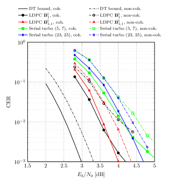
Figure 3: Comparison between LDPC codes over $\mathbb{F}_{8}$ with base matrices $\mathbf{B}^{\mathrm{I}}_{1}$ and ${\mathbf{B}}^{\mathrm{I}}_{1,1}$ with a serial turbo scheme, combined with 8-PSK modulation, code rate ${1}/{2}$, $N=160$ symbols and phase-noise having $\sigma_{\Delta}=2^{\circ}$ for the non-coherent case.

Example 2 ($R_{c}=2/3$, $8$-DPSK).

Step 1 of the protograph search for the Wiener phase noise channel yields the set $\mathcal{M}_{e}$ of $1\times 3$ base matrices. Iterative thresholds for all elements are given in Table IV for both the coherent and non-coherent channels. The Shannon limit for the coherent case is $\left(E_{b}/N_{0}\right)_{\mathsf{c}}^{\mathsf{Sh}}=2.76$  dB. For the non-coherent channel $\left(E_{b}/N_{0}\right)_{\mathsf{nc}}^{\mathsf{Sh}}=3.15$  dB. We find that the protograph with base matrix $\mathbf{B}^{\mathrm{II}}_{1}=[2~{}2~{}1]$ has the best threshold $\left(E_{b}/N_{0}\right)_{\mathsf{nc}}^{*}=3.81$ dB among all $7$ candidates in Table IV. We build out of it a rate-$2/3$ code with parameters $(120,80)$ and plot the CER versus $E_{b}/N_{0}$ on both the coherent and non-coherent AWGN channels in Figure 4. We observe from the figure that the gap to the DT bounds is around 1 dB, respectively. No visible error floor is present at the target block error probability.

TABLE IV: Iterative decoding thresholds for the non-coherent and coherent AWGN channel for $8$-DPSK modulation and rate-$2/3$ protographs.

	Base Matrix	$\left(E_{b}/N_{0}\right)_{\mathsf{nc}}^{*}$ [dB]	$\left(E_{b}/N_{0}\right)_{\mathsf{c}}^{*}$ [dB]
$\mathbf{B}^{\mathrm{II}}_{1}$	$[2\ 2\ 1]$	3.81	3.44
$\mathbf{B}^{\mathrm{II}}_{2}$	$[3\ 2\ 1]$	4.15	3.77
$\mathbf{B}^{\mathrm{II}}_{3}$	$[3\ 3\ 1]$	4.62	4.21
$\mathbf{B}^{\mathrm{II}}_{4}$	$[2\ 2\ 2]$	4.42	4.02
$\mathbf{B}^{\mathrm{II}}_{5}$	$[3\ 2\ 2]$	4.80	4.37
$\mathbf{B}^{\mathrm{II}}_{6}$	$[3\ 3\ 2]$	5.19	4.75
$\mathbf{B}^{\mathrm{II}}_{7}$	$[3\ 3\ 3]$	5.55	5.09

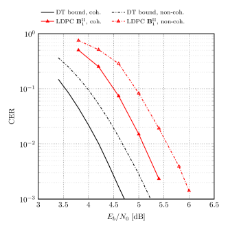
Figure 4: Simulation results of an LDPC code over $\mathbb{F}_{8}$ with base matrix $\mathbf{B}^{\mathrm{II}}_{1}$ combined with 8-DPSK modulation, code rate $2/3$, $N=120$ symbols and phase-noise with $\sigma_{\Delta}=2^{\circ}$ for the non-coherent case.

Example 3 ($R_{c}=3/4$, $16$-DPSK).

Step 1 of the protograph search yields a set $\mathcal{M}_{e}$ of $1\times 4$ base matrices. Its elements with the corresponding iterative decoding thresholds are given in Table V. The Shannon limit for the coherent case is $\left(E_{b}/N_{0}\right)_{\mathsf{c}}^{\mathsf{Sh}}=6.73$  dB. For the non-coherent channel $\left(E_{b}/N_{0}\right)_{\mathsf{nc}}^{\mathsf{Sh}}=7.12$  dB. We find that the base matrix $\mathbf{B}^{\mathrm{III}}_{1}=[2~{}2~{}2~{}1]$ has the best threshold $\left(E_{b}/N_{0}\right)_{\mathsf{nc}}^{*}=8.24$ dB for the non-coherent phase noise channel. We observe from the table that an ultra-sparse LDPC code with regular VN degrees of two would have $0.5$ dB worse threshold. A rate-$3/4$ $(128,96)$ LDPC code is obtained from it and its CER versus $E_{b}/N_{0}$ curve is depicted in Figure 5, together with the DT bound for the coherent and non-coherent AWGN channel. We observe from the figure a gap with respect to the DT bound of around $1.2$ dB.

TABLE V: Iterative decoding thresholds for the non-coherent and coherent AWGN channel for $16$-DPSK modulation and rate-$3/4$ protographs.

	Base Matrix	$\left(E_{b}/N_{0}\right)_{\mathsf{nc}}^{*}$ [dB]	$\left(E_{b}/N_{0}\right)_{\mathsf{c}}^{*}$ [dB]
$\mathbf{B}^{\mathrm{III}}_{1}$	$[2\ 2\ 2\ 1]$	8.24	7.85
$\mathbf{B}^{\mathrm{III}}_{2}$	$[3\ 2\ 2\ 1]$	8.57	8.16
$\mathbf{B}^{\mathrm{III}}_{3}$	$[3\ 3\ 2\ 1]$	8.95	8.50
$\mathbf{B}^{\mathrm{III}}_{4}$	$[3\ 3\ 3\ 1]$	9.31	8.83
$\mathbf{B}^{\mathrm{III}}_{5}$	$[2\ 2\ 2\ 2]$	8.76	8.33
$\mathbf{B}^{\mathrm{III}}_{6}$	$[2\ 2\ 2\ 3]$	9.08	8.62
$\mathbf{B}^{\mathrm{III}}_{7}$	$[3\ 3\ 2\ 2]$	9.40	8.93
$\mathbf{B}^{\mathrm{III}}_{8}$	$[3\ 3\ 3\ 2]$	9.71	9.19
$\mathbf{B}^{\mathrm{III}}_{9}$	$[3\ 3\ 3\ 3]$	9.97	9.45

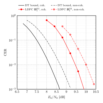
Figure 5: Simulation results of an LDPC code over $\mathbb{F}_{16}$ with base matrix $\mathbf{B}^{\mathrm{III}}_{1}$ combined with 16-PSK modulation, code rate $3/4$, $N=128$ symbols and phase-noise having $\sigma_{\Delta}=1^{\circ}$ for the non-coherent case.

VI Conclusions

In this work, we investigate the design of non-binary protograph LDPC codes for the Wiener phase noise channel. We consider the serial concatenation of an outer $m$-ary LDPC code over the finite field of order $m$ and $m$-DPSK, and target transmission of short blocks in the order of a few hundred symbols. Decoding of the concatenated scheme is performed in a turbo-like fashion where a detector and decoder iteratively exchange beliefs among each other. We give a finite-length benchmark, namely the DT bound, both for the coherent and non-coherent case. We show that, with a proper protograph LDPC code design, a performance of $1.2$ dB or less from the DT bound is achieved down to a CER of $10^{-3}$, even in the presence of strong phase noise. All our designs are robust with respect to phase noise, in the sense that they nearly show the same gap to the respective bounds for both the coherent and non-coherent setup. Furthermore, we observe that the protographs obtained for the Wiener phase noise channel are also the ones which have the best thresholds among all investigated protographs on the coherent channel.

References

- [1] International Telecommunication Union, “IMT Vision-Framework and overall objectives of the future development of IMT for 2020 and beyond,” Recommendation ITU-R M.2083-0, 2015.
- [2] A. Osseiran, F. Boccardi, V. Braun, K. Kusume, P. Marsch, M. Maternia, O. Queseth, M. Schellmann, H. Schotten, H. Taoka, H. Tullberg, M. A. Uusitalo, B. Timus, and M. Fallgren, “Scenarios for 5G mobile and wireless communications: the vision of the METIS project,” IEEE Commun. Mag., vol. 52, no. 5, pp. 26–35, May 2014.
- [3] G. Durisi, T. Koch, and P. Popovski, “Toward massive, ultrareliable, and low-latency wireless communication with short packets,” Proc. IEEE, vol. 104, no. 9, pp. 1711–1726, Sep. 2016.
- [4] D. Divsalar and M. K. Simon, “Multiple-symbol differential detection of MPSK,” IEEE Trans. Commun., vol. 38, no. 3, pp. 300–308, Mar. 1990.
- [5] G. Colavolpe, A. Barbieri, and G. Caire, “Algorithms for iterative decoding in the presence of strong phase noise,” IEEE J. Sel. Areas Commun., vol. 23, no. 9, pp. 1748–1757, Sep. 2005.
- [6] G. Colavolpe, “Communications over phase-noise channels: A tutorial review,” Int. J. Satell. Commun. Network., vol. 32, pp. 167–185, May/Jun. 2014, article first published online: Jul. 2013.
- [7] G. Colavolpe and R. Raheli, “Theoretical analysis and performance limits of noncoherent sequence detection of coded PSK,” IEEE Trans. Inf. Theory, vol. 46, pp. 1483–1494, Jul. 2000.
- [8] M. Peleg, S. Shamai, and S. Galan, “Iterative decoding for coded noncoherent MPSK communications over phase-noisy AWGN channel,” IEE Proceedings - Communications, vol. 147, no. 2, pp. 87–95, Apr. 2000.
- [9] P. Hoeher and J. Lodge, “Turbo DPSK: iterative differential PSK demodulation and channel decoding,” IEEE Trans. Commun., vol. 47, no. 6, pp. 837–843, Jun. 1999.
- [10] S. Karuppasami and W. Cowley, “Construction and iterative decoding of LDPC codes over rings for phase-noisy channels,” EURASIP Journal on Wireless Communications and Networking, vol. 2008, pp. 1–9, Jan. 2008.
- [11] B. Matuz, G. Liva, E. Paolini, M. Chiani, and G. Bauch, “Low-rate non-binary LDPC codes for coherent and blockwise non-coherent AWGN channels,” IEEE Trans. Commun., vol. 61, no. 10, pp. 4096–4107, Oct. 2013.
- [12] A. Barbieri and G. Colavolpe, “Soft-output decoding of rotationally invariant codes over channels with phase noise,” IEEE Trans. Commun., vol. 55, no. 10, pp. 2033–2033, Oct. 2007.
- [13] C. Piat-Durozoi, C. Poulliat, N. Thomas, M. Boucheret, and G. Lesthievent, “On sparse graph coding for coherent and noncoherent demodulation,” in Proc. IEEE Int. Symp. Inf. Theory, Jun. 2017, pp. 2905–2909.
- [14] M. Franceschini, G. Ferrari, R. Raheli, and A. Curtoni, “Serial concatenation of LDPC codes and differential modulations,” IEEE J. Sel. Areas Commun., vol. 23, no. 9, pp. 1758–1768, Sep. 2005.
- [15] A. Barbieri and G. Colavolpe, “On the information rate and repeat-accumulate code design for phase noise channels,” IEEE Trans. Commun., vol. 59, no. 12, pp. 3223–3228, Dec. 2011.
- [16] S. ten Brink and G. Kramer, “Design of repeat-accumulate codes for iterative detection and decoding,” IEEE Trans. Signal Process., vol. 51, no. 11, pp. 2764–2772, Nov. 2003.
- [17] J. L. Massey and T. Mittelholzer, “Convolutional codes over rings,” in Proc. 4th Joint Swedish-Soviet Int. Workshop on Inf. Theory, Gotland, Sweden, Aug. 1989, pp. 14–18.
- [18] R. Filho and P. Farrell, “Coded modulation with convolutional codes over rings,” in Proc. EUROCODE ’90, ser. Lecture notes on computer science, Udine, Italy, Nov. 1990, pp. 271–280.
- [19] S. Karuppasami, W. G. Cowley, and S. S. Pietrobon, “LDPC code construction and iterative receiver techniques for channels with phase noise,” in VTC Spring 2008 - IEEE Vehicular Technology Conference, May 2008, pp. 2892–2896.
- [20] D. Sridhara and T. Fuja, “LDPC codes over rings for PSK modulation,” IEEE Trans. Inf. Theory, vol. 51, no. 9, pp. 3209–3220, Sep. 2005.
- [21] T. Ninacs, B. Matuz, G. Liva, and G. Colavolpe, “Non-binary LDPC coded DPSK modulation for phase noise channels,” in Proc. IEEE Int. Conf. Commun., Paris, France, May 2017, pp. 1–6.
- [22] M. Davey and D. MacKay, “Low density parity check codes over GF,” IEEE Commun. Lett., vol. 2, no. 6, pp. 70–71, Jun. 1998.
- [23] B.-Y. Chang, L. Dolecek, and D. Divsalar, “EXIT chart analysis and design of non-binary protograph-based LDPC codes,” in MILCOM 2011 Military Communications Conference, Baltimore, MD, USA, Nov. 2011, pp. 566–571.
- [24] L. Costantini, B. Matuz, G. Liva, E. Paolini, and M. Chiani, “Non-binary protograph LDPC codes for space communications,” Int. J. Satell. Commun. Network., vol. 30, no. 2, pp. 43–51, Mar. 2012.
- [25] C. Poulliat, M. Fossorier, and D. Declercq, “Design of regular -LDPC codes over GF using their binary images,” IEEE Trans. Commun., vol. 56, no. 10, pp. 1626–1635, Oct. 2008.
- [26] F. Kschischang, B. Frey, and H.-A. Loeliger, “Factor graphs and the sum-product algorithm,” IEEE Trans. Inf. Theory, vol. 47, no. 2, pp. 498–519, Feb 2001.
- [27] L. R. Bahl, J. Cocke, F. Jelinek, and J. Raviv, “Optimal decoding of linear codes for minimizing symbol error rate,” IEEE Trans. Inf. Theory, vol. 20, no. 2, pp. 284–287, Mar. 1974.
- [28] D. Declercq and M. Fossorier, “Decoding algorithms for nonbinary LDPC codes over GF,” IEEE Trans. Commun., vol. 55, no. 4, pp. 633–643, Apr. 2007.
- [29] H. Wymeersch, H. Steendam, and M. Moeneclaey, “Log-domain decoding of LDPC codes over GF(),” in Proc. IEEE Int. Conf. Commun., vol. 2, Paris, France, Jun. 2004, pp. 772–776.
- [30] L. Sassatelli and D. Declercq, “Nonbinary hybrid LDPC codes,” vol. 56, no. 10, pp. 5314–5334, Oct. 2010.
- [31] D. M. Arnold, H. A. Loeliger, P. O. Vontobel, A. Kavcic, and W. Zeng, “Simulation-based computation of information rates for channels with memory,” IEEE Trans. Inf. Theory, vol. 52, no. 8, pp. 3498–3508, Aug. 2006.
- [32] Y. Polyanskiy, H. V. Poor, and S. Verdú, “Channel coding rate in the finite blocklength regime,” IEEE Trans. Inf. Theory, vol. 56, no. 5, pp. 2307–2359, May 2010.
- [33] J. Thorpe, “Low-density parity-check (LDPC) codes constructed from protographs,” NASA JPL, Pasadena, CA, USA, IPN Progress Report 42-154, Aug. 2003.
- [34] X.-Y. Hu, E. Eleftheriou, and D. M. Arnold, “Progressive edge-growth Tanner graphs,” in Proc. IEEE Global Telecommun. Conf., San Antonio, TX, USA, Nov. 2001, pp. 995–1001.
- [35] B. Y. Chang, D. Divsalar, and L. Dolecek, “Non-binary protograph-based LDPC codes for short block-lengths,” in Proc. IEEE Inf. Theory Workshop, Lausanne, Switzerland, Sep. 2012, pp. 282–286.
- [36] A. Bennatan and D. Burshtein, “Design and analysis of nonbinary LDPC codes for arbitrary discrete-memoryless channels,” IEEE Trans. Inf. Theory, vol. 52, no. 2, pp. 549–583, Feb. 2006.
- [37] G. Liva and M. Chiani, “Protograph LDPC codes design based on EXIT analysis,” in Proc. IEEE Global Telecommun. Conf., Washington, DC, USA, Nov. 2007, pp. 3250–3254.
- [38] D. MacKay, Information Theory, Inference & Learning Algorithms. New York, NY, USA: Cambridge University Press, 2002.
- [39] B. Matuz, E. Paolini, F. Zabini, and G. Liva, “Non-binary LDPC code design for the poisson PPM channel,” IEEE Trans. Commun., vol. 65, no. 11, pp. 4600–4611, Nov. 2017.
- [40] S. Benedetto, D. Divsalar, G. Montorsi, and F. Pollara, “Serial concatenation of interleaved codes: performance analysis, design, and iterative decoding,” IEEE Trans. Inf. Theory, vol. 44, no. 3, pp. 909–926, May 1998.
- [41] A. Shokrollahi and R. Storn, “Design of efficient erasure codes with differential evolution,” in Differential Evolution. Springer, 2005, pp. 413–427.
- [42] X. Y. Hu and E. Eleftheriou, “Binary representation of cycle tanner-graph GF() codes,” in Proc. IEEE Int. Conf. Commun., vol. 1, Paris, France, Jun. 2004, pp. 528–532.
- [43] G. Liva, E. Paolini, and M. Chiani, “Bounds on the error probability of block codes over the q-ary erasure channel,” IEEE Trans. Commun., vol. 61, no. 6, pp. 2156–2165, Jun. 2013.
- [44] Digital Video Broadcasting (DVB); Second Generation Framing Structure, Channel Coding and Modulation Systems for Broadcasting, Interactive Services, News Gathering and Other Broadband Satellite Applications (DVB-S2), ETSI EN 302 307 v1.2.1, ETSI European Standard (Telecommunications series), Aug. 2009.
- [45] “TSG RAN WG1 meeting no. 85 R1-164041,” 3GPP, Nanjing, China, Tech. Rep., May 2016.