Branching Fractions of the $\bm{X(3872)}$

Abstract

The recoil momentum spectrum from the decay $B^{+}\to K^{+}+\mathrm{anything}$ has recently been measured by the BaBar collaboration. The spectrum has a peak with invariant mass near the mass of the $X(3872)$ meson. The preliminary measurement by the BaBar collaboration implies that its branching fraction into $J/\psi\,\pi^{+}\pi^{-}$ is about 4%. We emphasize that this is the branching fraction for the entire resonance feature from $B^{+}$-to-$K^{+}$ transitions, which includes a $D^{*0}\bar{D}^{0}$ and $D^{0}\bar{D}^{*0}$ threshold enhancement as well as a possible bound state below the threshold or a virtual state. If the $X$ is a bound state of charm mesons, its branching fraction into $J/\psi\,\pi^{+}\pi^{-}$ should be considerably larger than that of the $X$ resonance feature. We use measurements of branching ratios of the $X$ to put an upper bound on this branching fraction of 33%. We also constrain the parameters of the simplest plausible model for the line shapes of the $X$ using the precise measurement of the resonance energy of the $X$ and an estimate of the branching fraction into $D^{0}\bar{D}^{0}\pi^{0}$ and $D^{0}\bar{D}^{0}\gamma$ from the $X$ resonance feature from $B^{+}$-to-$K^{+}$ transitions.

I Introduction

Dozens of exotic heavy hadrons whose constituents include a heavy quark and its antiquark have been discovered in high energy physics experiments since the beginning of the century Chen:2016qju ; Hosaka:2016pey ; Lebed:2016hpi ; Esposito:2016noz ; Guo:2017jvc ; Ali:2017jda ; Olsen:2017bmm ; Karliner:2017qhf ; Yuan:2018inv ; Brambilla:2019esw . The first one to be discovered was the $X(3872)$ meson, whose constituents include a charm quark and its antiquark. It was discovered by the Belle Collaboration in 2003 through its decay into $J/\psi\,\pi^{+}\pi^{-}$ Choi:2003ue . Its $J^{PC}$ quantum numbers were finally determined by the LHCb collaboration in 2013 to be $1^{++}$ Aaij:2013zoa . Its mass is extremely close to the $D^{*0}\bar{D}^{0}$ scattering threshold, with recent measurements indicating that the difference is at most about 0.2 MeV Tanabashi:2018oca . These facts suggest that $X(3872)$ is a weakly bound S-wave charm-meson molecule with the flavor structure

$$\big{|}X(3872)\rangle=\frac{1}{\sqrt{2}}\Big{(}\big{|}D^{*0}\bar{D}^{0}\big{\rangle}+\big{|}D^{0}\bar{D}^{*0}\big{\rangle}\Big{)}.$$ (1)

However, there are alternative models for the $X$ that have not been excluded Chen:2016qju ; Hosaka:2016pey ; Lebed:2016hpi ; Esposito:2016noz ; Guo:2017jvc ; Ali:2017jda ; Olsen:2017bmm ; Karliner:2017qhf ; Yuan:2018inv ; Brambilla:2019esw . The $X$ has been observed in the constituent decay modes $D^{0}\bar{D}^{0}\pi^{0}$ and $D^{0}\bar{D}^{0}\gamma$, which receive contributions from the decay of a constituent $D^{*0}$ or $\bar{D}^{*0}$. It has also been observed in five short-distance decay modes, including $J/\psi\,\pi^{+}\pi^{-}$, whose ultimate final states include particles with momenta larger than the pion mass. Despite all the information on its decays, there is as of yet no consensus on the nature of the $X$.

There may be aspects of the production of $X$ that are more effective at discriminating between models than its decays. If $X$ is a weakly bound charm-meson molecule, its production can proceed by the creation of a charm-meson pair $D^{*0}\bar{D}^{0}$ or $D^{0}\bar{D}^{*0}$ at short distances of order $1/m_{\pi}$ or smaller, where $m_{\pi}$ is the pion mass, followed by the binding of the charm mesons into $X$ at longer distances. The production of $X$ can also proceed by the creation of a charm-meson pair $D^{*}\bar{D}^{*}$ at short distances followed by the rescattering of the charm mesons into $X$ and a pion Braaten:2018eov ; Braaten:2019yua ; Braaten:2019sxh or into $X$ and a photon Dubynskiy:2006cj ; Guo:2019qcn ; Braaten:2019gfj at longer distances. There are Feynman diagrams for such rescattering processes in which three charm mesons whose lines form a triangle can all be near their mass shells simultaneously. A triangle singularity therefore produces a narrow peak in the $X\pi$ or $X\gamma$ invariant mass near the $D^{*}\bar{D}^{*}$ threshold. Guo pointed out that any high-energy process that can create an S-wave $D^{*0}\bar{D}^{*0}$ pair at short distances will also produce $X\gamma$ with a narrow peak near the $D^{*0}\bar{D}^{*0}$ threshold due to a charm-meson triangle singularity Guo:2019qcn . We had noted previously that rescattering of an S-wave $D^{*}\bar{D}^{*}$ pair produces a narrow peak in the $X\pi$ invariant mass near the $D^{*}\bar{D}^{*}$ threshold in hadron collisions Braaten:2018eov ; Braaten:2019sxh and in $B$ meson decay into $KX\pi$ Braaten:2019yua , without noting the connection to triangle singularities. In Ref. Braaten:2019gfj , we calculated the cross section for electron-positron annihilation into $X\gamma$ near the $D^{*0}\bar{D}^{*0}$ threshold, where rescattering of a P-wave $D^{*0}\bar{D}^{*0}$ pair produces a narrow peak due to a triangle singularity. The peaks in the $X\pi$ or $X\gamma$ invariant mass from charm-meson triangle singularities provide smoking guns for the identification of the $X$ as a charm-meson molecule.

It is important to have quantitative predictions for the height, width, and shape of the peaks from the charm-meson triangle singularities. If the $X$ is a weakly bound charm-meson molecule, the height of the peak in a specific decay mode is controlled by the binding energy of the $X$ and by its branching fraction into that decay mode. The BaBar collaboration has recently determined the inclusive branching fraction of the $B^{+}$ meson into $K^{+}$ plus the $X$ resonance by measuring the recoil momentum spectrum of the $K^{+}$ Wormser . The preliminary result implies that the branching fraction of the entire $X$ resonance feature into $J/\psi\,\pi^{+}\pi^{-}$ is about 4%. This small branching fraction may suggest that it could be difficult to observe the peak from a charm-meson triangle singularity in the $J/\psi\,\pi^{+}\pi^{-}$ decay mode. However the $X$ resonance feature includes a threshold enhancement in the production of $D^{*0}\bar{D}^{0}$ and $D^{0}\bar{D}^{*0}$ as well as a possible narrow peak from the $X$ bound state. We emphasize in this paper that the branching fraction of the $X$ bound state into $J/\psi\,\pi^{+}\pi^{-}$ should be considerably larger than the corresponding branching fraction of the $X$ resonance feature.

We begin in Section II by explaining why branching fractions of a bound state must be the same for all short-distance production mechanisms. In Section III, we describe the simplest plausible model for the line shapes of the $X$ resonance. In Section IV, we discuss the short-distance production of the $X$ resonance and present a simple theoretical prescription for the resonance energy. We determine the resonance energy analytically for the simplest model for the $X$ line shapes in three limits. In Section V, we discuss branching fractions for the $X$ resonance feature and for the $X$ bound state. We use previous experimental results to estimate the branching fraction for the $X$ resonance feature from $B^{+}$-to-$K^{+}$ transitions into short-distance decay modes. We use our estimate for that branching fraction combined with the current result for the $X$ resonance energy to constrain the parameters of the simplest model for the $X$ line shapes. We summarize our results in Section VI.

II Factorization in Short-distance Production

We consider pairs of particles with coupled S-wave scattering channels that we label by an index $i$ and that have nearby scattering thresholds. We are particularly interested in the case of an S-wave resonance near the scattering threshold for the lowest channel, which we take to be at the energy $E=0$. The transition rates between channels can be expressed in terms of scattering amplitudes $f_{ij}(E)$ that depend on the center-of-mass energy $E$. The optical theorem for the scattering amplitudes that follows from the unitarity of the S-matrix is

$$2\,\mathrm{Im}\big{[}f_{ij}(E)\big{]}=\sum_{k}f_{ik}(E)\,f_{jk}(E)^{*}.$$ (2)

If there is a resonance, the scattering amplitudes for all the coupled channels have a pole at the same complex energy $E_{X}-i\Gamma_{X}/2$, where $E_{X}$ and $\Gamma_{X}$ are real. At complex energies $E$ near the pole, the scattering amplitudes can be expressed in the factored form

$$f_{ij}(E)\approx\frac{-c_{i}\,c_{j}}{E-E_{X}+i\Gamma_{X}/2},$$ (3)

where the energy-independent constants $c_{i}$’s are required to be real by time-reversal symmetry. If the pole is on the physical sheet of the complex energy $E$, the resonance is referred to as a bound state. If the pole is on a different sheet of $E$, the resonance is referred to as a virtual state. A narrow bound state is one for which the pole energy satisfies $E_{X}<0$ and $\Gamma_{X}>0$ with $|E_{X}|$ significantly larger than $\Gamma_{X}/2$. In this case, $|E_{X}|$ can be interpreted as the binding energy and $\Gamma_{X}$ can be interpreted as the decay width of the bound state. Only in the case of a narrow bound state are the expressions for the scattering amplitudes near the pole in Eq. (3) good approximations over a real range of the energy $E$.

There may be short-distance production mechanisms for the pairs of particles that involve momentum scales much larger than those provided by $E_{X}$, $\Gamma_{X}$, and the energy differences between scattering thresholds. The amplitude for the short-distance production of a pair of particles in the scattering channel $k$ can be expressed in the factored form $\sum_{i}B_{i}\,f_{ik}(E)$, where the short-distance factor $B_{i}$ is insensitive to the energy $E$. In the case of S-wave production channels, the $B_{i}$’s are constants. Different short-distance production mechanisms will have different factors $B_{i}$. The inclusive production rate summed over channels $k$ can be expressed as

$$\frac{dR}{dE}=\sum_{k}\Big{(}\sum_{i}B_{i}\,f_{ik}(E)\Big{)}\,\Big{(}\sum_{j}B_{j}\,f_{jk}(E)\Big{)}^{*}.$$ (4)

The optical theorem in Eq. (2) implies that the inclusive production rate can be expressed in the factored form

$$\frac{dR}{dE}=2\sum_{ij}B_{i}\,\mathrm{Im}\big{[}f_{ij}(E)\big{]}\,{B_{j}}^{*}.$$ (5)

The S-wave resonance produces an enhancement in the inclusive production rate near the threshold. We refer to the entire resonantly enhanced contribution as the resonance feature. The energy dependence of $dR/dE$ defines the inclusive line shape. A unique feature of a near-threshold S-wave resonance is that the resonance feature includes a peak in the production rate of pairs of particles just above the threshold, which we refer to as a threshold enhancement. The resonance feature may also include contributions below the threshold from a bound state or a virtual state.

In the case of a narrow bound state, the inclusive production rate has a narrow peak below the threshold with a maximum near $E_{X}$ and a width in $E$ of about $\Gamma_{X}$. The pole approximation for the scattering amplitude in Eq. (3) can be used to express the inclusive production rate in Eq. (5) at real energies $E$ near the peak in a factored form:

$$\frac{dR}{dE}\approx\Big{(}\sum_{i}B_{i}c_{i}\Big{)}\frac{\Gamma_{X}}{(E-E_{X})^{2}+\Gamma_{X}^{2}/4}\Big{(}\sum_{j}B_{j}c_{j}\Big{)}^{*}.$$ (6)

The decay width $\Gamma_{X}$ in the numerator can be expanded as a sum of the partial widths of all the decay modes $k$ of the bound state: $\Gamma_{X}=\sum_{k}\Gamma_{X\to k}$. The production rate $dR_{k}/dE$ in a specific decay mode $k$ can be expressed in the same factored form in Eq. (6) with $\Gamma_{X}$ in the numerator replaced by $\Gamma_{X\to k}$. The branching fraction $\Gamma_{X\to k}/\Gamma_{X}$ can also be expressed as the ratio of an integral of $dR_{k}/dE$ over an integral of $dR/dE$, where the integrals are over the narrow peak from the bound state. The factorized form of Eq. (6) guarantees that such a branching fraction is independent of the production mechanism.

The independence of the branching fractions on the production mechanism is guaranteed only in the case of a narrow bound state and only for branching fractions obtained by integrating over the narrow bound-state peak. In the case of a virtual state or a bound state that is not narrow, a branching fraction defined by a ratio of integrals should be expected to depend on the production mechanism. Even in the case of a narrow bound state, if the integration region is extended to include the threshold enhancement, a branching fraction defined by a ratio of integrals should be expected to depend on the production mechanism.

III Simplest Model for $\bm{X}$ Line Shapes

In the case of the $X(3872)$ resonance, the particles are charm mesons. We denote the masses of $D^{*0}$ and $D^{0}$ by $M_{*0}$ and $M_{0}$, respectively. We denote the masses of $D^{*+}$ and $D^{+}$ by $M_{*1}$ and $M_{1}$, respectively. The reduced mass of $D^{*0}\bar{D}^{0}$ is $\mu=M_{*0}M_{0}/(M_{*0}\!+\!M_{0})=967$ MeV. The difference between the scattering thresholds for $D^{*+}D^{-}$ and $D^{*0}\bar{D}^{0}$ is $\delta=(M_{*1}\!+\!M_{1})-(M_{*0}\!+\!M_{0})=8.2$ MeV. The decay width of the $D^{*0}$ can be predicted from measurements of $D^{*}$ decays: $\Gamma_{*0}=(55.9\pm 1.6)$ keV Rosner:2013sha . The corresponding momentum scale is $\sqrt{\mu\Gamma_{*0}}=7.4$ MeV. The present value of the difference $E_{X}$ between the mass of the $X$ and the energy of the $D^{*0}\bar{D}^{0}$ scattering threshold is Tanabashi:2018oca

$$E_{X}\equiv M_{X}-(M_{*0}\!+\!M_{0})=(+0.01\pm 0.18)~{}\mathrm{MeV}.$$ (7)

This value has been obtained from measurements in the $J/\psi\,\pi^{+}\pi^{-}$ decay mode. The central value of $E_{X}$ is essentially at the $D^{*0}\bar{D}^{0}$ scattering threshold. The value of $E_{X}$ lower by $1\sigma$ corresponds to a bound state with binding energy $|E_{X}|=0.17$ MeV.

The line shape for the $X(3872)$ in the $D^{0}\bar{D}^{0}\pi^{0}$ decay mode from the decay $B\to K(D^{0}\bar{D}^{0}\pi^{0})$ has been measured by the Belle collaboration Gokhroo:2006bt . The distribution in the energy $E$ defined by the difference between the $D^{0}\bar{D}^{0}\pi^{0}$ invariant mass and the $D^{*0}\bar{D}^{0}$ threshold has a peak at $E=4.2^{+0.8}_{-1.7}$ MeV. The fitted energy distribution decreases to a local minimum near 10 MeV before increasing. The distribution up to that minimum can be identified with the $X$ resonance feature in the $D^{0}\bar{D}^{0}\pi^{0}$ decay mode. The resolution was insufficient to resolve any further substructure in the resonance feature.

There have been many previous theoretical studies of the line shapes of the $X(3872)$ resonance. The earliest such studies were carried out by Voloshin Voloshin:2003nt ; Voloshin:2007hh . The simplest analytic model for the line shapes considers only the single resonant channel with a neutral-charm-meson pair Braaten:2007dw . More elaborate analytic models take into account the coupling to a charmonium state with quantum numbers $1^{++}$ that can be identified with the $\chi_{c1}(2P)$ Hanhart:2007yq ; Zhang:2009bv ; Kalashnikova:2009gt ; Artoisenet:2010va , the coupling to a charged-charm-meson pair Braaten:2007ft ; Artoisenet:2010va ; Hanhart:2011jz ; Kang:2016jxw , and the coupling to the $J/{\psi}\,\omega$ channel Braaten:2013poa . There have also been efforts to take into account the $D\bar{D}\pi$ channels by using an effective field theory for charm mesons and pions called XEFT Fleming:2007rp ; Braaten:2015tga or by solving Lippmann-Schwinger equations numerically Baru:2011rs ; Schmidt:2018vvl .

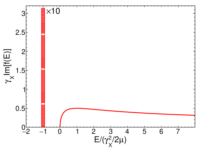
Figure 1: Line shape $\mathrm{Im}[f_{X}(E+i\epsilon)]$ in Eq. (9) as a function of the energy $E$. The resonance feature includes a threshold enhancement from production of the pair of particles above the scattering threshold at $E=0$. If $\gamma_{X}>0$, the resonance feature also includes a delta function from production of the bound state below the scattering threshold. It is represented by the tall rectangle whose area should be multiplied by 10.

For particles with short-range interactions that produce an S-wave resonance sufficiently close to the scattering threshold, the scattering amplitude at very low energy has the simple universal form Braaten:2004rn

$$f(E)=\frac{1}{-\gamma_{X}+\sqrt{-2\mu(E+i\epsilon)}},$$ (8)

where $\mu$ is the reduced mass of the pair of particles and $E$ is their total energy relative to the scattering threshold. Exact unitarity requires the inverse scattering length $\gamma_{X}$ to be real. The inclusive line shape is

$$\mathrm{Im}[f_{X}(E+i\epsilon)] = \frac{\pi\gamma_{X}}{\mu}\delta(E+\gamma_{X}^{2}/2\mu)\,\theta(\gamma_{X})\qquad(E<0),$$ (9a)

$$= \frac{\sqrt{2\mu E}}{\gamma_{X}^{2}+2\mu E}\qquad\qquad\qquad\qquad~{}(E>0).$$ (9b)

Eq. (9b) implies that the maximum of the threshold enhancement is at $E=+\gamma_{X}^{2}/2\mu$. Eq. (9a) implies that if $\gamma_{X}>0$, there is also a delta function at the negative energy $E_{X}=-\gamma_{X}^{2}/2\mu$ from production of the bound state. The threshold enhancement together with the delta function (if there is one) forms the resonance feature, which is illustrated in Fig. 1. Note that the integral of the line shape in Eq. (9b) up to an energy $E_{\mathrm{max}}$ increases as $E_{\mathrm{max}}^{1/2}$. In contrast to the line shape of a Breit-Wigner resonance, the integral diverges as $E_{\mathrm{max}}\to\infty$. This behavior introduces complications in the definitions of some resonance properties.

In the case of the $X(3872)$, the superposition of neutral charm-meson pairs in Eq. (1) has a resonance in the S-wave $1^{++}$ channel. The nearest threshold for a coupled channel is that for the charged-charm meson pairs, which is higher by 8.2 MeV. The simplest plausible model for the resonant scattering amplitude $f(E)$ can be obtained from the universal amplitude in Eq. (8) by making two changes Braaten:2007dw :

• The effects of the width of the $D^{*0}$ are taken into account by replacing $E+i\epsilon$ by $E+i\Gamma_{*0}/2$.

• The effects of short-distance decay modes are taken into account by allowing the real parameter $\gamma_{X}$ to have a positive imaginary part.

The resulting scattering amplitude is

$$f(E)=\frac{1}{-\gamma_{X}+\sqrt{-2\mu(E+i\Gamma_{*0}/2)}}.$$ (10)

The only undetermined parameter in the amplitude is the complex inverse scattering length $\gamma_{X}$. The real and imaginary parts of $\gamma_{X}$ are both determined by the physics at short distances. However $\mathrm{Re}[\gamma_{X}]$ is sensitive to the fine tuning of the physics at short distances. For the purpose of order-of-magnitude estimates, we will assume $\mathrm{Im}[\gamma_{X}]$ is order $\sqrt{\mu\Gamma_{*0}}$. The real part of $\gamma_{X}$ can range from positive values much larger than $\sqrt{\mu\Gamma_{*0}}$ to negative values with absolute value much larger than $\sqrt{\mu\Gamma_{*0}}$.

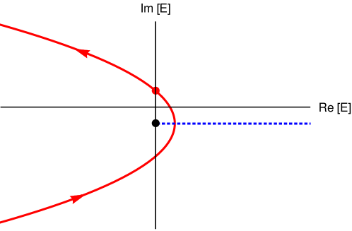
Figure 2: Analytic features of the scattering amplitude $f(E)$ in Eq. (10) in the plane of the complex energy $E$. The solid curve is the path of the pole as $\mathrm{Re}[\gamma_{X}]$ is varied with $\mathrm{Im}[\gamma_{X}]$ fixed. The arrows indicate the direction of increasing resonance energy $E_{X}$. The branch point at $-i\Gamma_{*0}/2$ for the square-root branch cut (dashed line) is marked by a dot. The dot on the solid curve marks the point on the second sheet where there is a zero-energy resonance with $E_{X}=0$. We have set $\mathrm{Im}[\gamma_{X}]=\sqrt{\mu\Gamma_{*0}}$.

The scattering amplitude in Eq. (10) is an analytic function of the complex energy $E$ with a square-root branch point at $E=-i\Gamma_{*0}/2$. We choose the branch cut to be along the line $\mathrm{Re}[E]>0$, $\mathrm{Im}[E]=-i\Gamma_{*0}/2$. The amplitude also has a pole at the energy $E_{\mathrm{pole}}=-\gamma_{X}^{2}/(2\mu)-i\Gamma_{*0}/2$. Its expression in terms of the real and imaginary parts of $\gamma_{X}$ is

$$E_{\mathrm{pole}}=-\frac{\mathrm{Re}[\gamma_{X}]^{2}-\mathrm{Im}[\gamma_{X}]^{2}}{2\mu}-\frac{i}{2}\left(\Gamma_{*0}+\frac{2\,\mathrm{Re}[\gamma_{X}]\,\mathrm{Im}[\gamma_{X}]}{\mu}\right).$$ (11)

The path of the pole in the plane of the complex energy $E$ as $\mathrm{Re}[\gamma_{X}]$ decreases with $\mathrm{Im}[\gamma_{X}]$ fixed is illustrated in Fig. 2. The pole crosses the branch cut when $\mathrm{Re}[\gamma_{X}]=0$. If $\mathrm{Re}[\gamma_{X}]>0$, the pole is on the physical sheet and the resonance is a bound state. If $\mathrm{Re}[\gamma_{X}]<0$, the pole is on the second sheet and the resonance is a virtual state. For complex energies $E$ near the pole, the scattering amplitude can be approximated by

$$f(E)\approx\frac{-\gamma_{X}/\mu}{E-E_{\mathrm{pole}}},$$ (12)

The inclusive production rate of the resonance through a mechanism that creates the constituents at short distances is proportional to $\mathrm{Im}[f(E)]$. The imaginary part of the scattering amplitude in Eq. (10) at a real energy $E$ can be expressed as

$$\mathrm{Im}\big{[}f(E)\big{]}=\big{|}f(E)\big{|}^{2}\left(\mathrm{Im}[\gamma_{X}]+\Big{[}\mu\sqrt{E^{2}+\Gamma_{*0}^{2}/4}+\mu E\Big{]}^{1/2}\right).$$ (13)

The unitarity condition $\mathrm{Im}[f(E)]\geq 0$ requires $\mathrm{Im}[\gamma_{X}]\geq 0$. The term in Eq. (13) with the factor $\mathrm{Im}[\gamma_{X}]$ can be interpreted as the contribution from the short-distance decay (SDD) channel, which consists of the decay modes whose ultimate final states include particles with momenta larger than $m_{\pi}$. The simplest model for the $X$ line shapes predicts that all the decay modes in the SDD channel have the same line shape proportional to $|f(E)|^{2}$. In the case of the $X$ resonance, $\mathrm{Im}[\gamma_{X}]$ can be expressed as the sum of positive contributions from $J/\psi\,\pi^{+}\pi^{-}$ and all the other decay modes in the SDD channel. There may also be small short-distance contributions from the $D^{0}\bar{D}^{0}\pi^{0}$ and $D^{0}\bar{D}^{0}\gamma$ decay modes. The other term in Eq. (13) (which has the factor in square brackets raised to the power $\tfrac{1}{2}$) can be interpreted as the contribution from the constituent decay (CD) channel, which consists of the decay modes whose ultimate final states are $D^{0}\bar{D}^{0}\pi^{0}$ and $D^{0}\bar{D}^{0}\gamma$. This simplest model for the $X$ line shapes predicts that the line shapes in the $D^{0}\bar{D}^{0}\pi^{0}$ and $D^{0}\bar{D}^{0}\gamma$ decay modes differ only by multiplicative constants whose ratio is the branching ratio of $D^{*0}$ into $D^{0}\pi^{0}$ over $D^{0}\gamma$. The line shape for the CD channel has a threshold enhancement from the production of $D^{*0}\bar{D}^{0}$ or $D^{0}\bar{D}^{*0}$ above their scattering threshold as well as contributions from the production of $D^{0}\bar{D}^{0}\pi^{0}$ or $D^{0}\bar{D}^{0}\gamma$ below that threshold.

Some aspects of a resonance feature are most conveniently quantified in terms of integrals of line shapes over the energy. If the inclusive line shape in Eq. (13) is integrated over the energy from $E_{\mathrm{min}}$ to $E_{\mathrm{max}}$, the integral diverges as $E_{\mathrm{min}}\to-\infty$ and as $E_{\mathrm{max}}\to+\infty$. It is therefore necessary to introduce an additional prescription for the resonance defined by the scattering amplitude in Eq. (10). A simple prescription for the resonance is to declare it to be the energy range between a specified energy $E_{\mathrm{min}}$ below the scattering threshold and a specified energy $E_{\mathrm{max}}$ above the threshold. Equivalently, we could declare the line shape to be given by Eq. (13) for $E_{\mathrm{min}}<E<E_{\mathrm{max}}$ and to be zero outside that interval. The sudden drops of the inclusive line shape from the function in Eq. (13) to 0 below $E_{\mathrm{min}}$ and above $E_{\mathrm{max}}$ emphasizes the crudeness of this model for the threshold enhancement. An alternative prescription for the resonance would be to smear the line shape in Eq. (13) using a Gaussian function of $E$ whose width could be chosen to mimic the experimental energy resolution. We choose to use the simpler prescription $E_{\mathrm{min}}<E<E_{\mathrm{max}}$ for the resonance, because it can be used to obtain analytic results for some properties of the resonance in certain limits.

In order to make quantitative predictions for properties of the resonance, we need to choose numerical values for $E_{\mathrm{min}}$ and $E_{\mathrm{max}}$. The energy range from $E_{\mathrm{min}}$ to $E_{\mathrm{max}}$ must be wide enough to cover most of the resonance. The values of $E_{\mathrm{max}}$ must be at most 8.2 MeV to avoid complications from the coupling to the charged-charm-meson-pair channel. The values of $|E_{\mathrm{min}}|$ and $E_{\mathrm{max}}$ must be less than $m_{\pi}^{2}/M_{D}\approx 10$ MeV to avoid contributions involving the large momentum scale $m_{\pi}$. We choose $E_{\mathrm{min}}$ and $E_{\mathrm{max}}$ rather arbitrarily to be the nearest relevant kinematic thresholds. We choose $E_{\mathrm{min}}$ to be the $D^{0}\bar{D}^{0}\pi^{0}$ threshold: $E_{\mathrm{min}}=-7.0$ MeV. We choose $E_{\mathrm{max}}$ to be the $D^{*+}D^{-}$ threshold: $E_{\mathrm{max}}=+8.2$ MeV.

IV Resonance energy

The difference between the line shape of a near-threshold S-wave resonance and that of a conventional resonance complicates the definition of the $X$ resonance energy. In this Section, we introduce a theoretical prescription for the resonance energy $E_{X}$. In the case of the simplest model for the $X$ lines shapes, we determine $E_{X}$ analytically in three limits.

A possible theoretical definition of a resonance energy, such as $E_{X}$ in Eq. (7), is the resonance-weighted average of the energy, which can be defined mathematically as a ratio of integrals. Such a definition is not applicable if the integrals do not converge, which is the case for a near-threshold S-wave resonance. An alternative theoretical definition of the resonance energy $E_{X}$ is the center of the resonance in a specified decay mode $k$, which can be defined mathematically by the condition that its contribution to the production rate receives equal contributions from the energy regions $E<E_{X}$ and $E>E_{X}$:

$$\int_{E_{\mathrm{min}}}^{E_{X}}\!\!\!dE\,\mathrm{Im}[f(E)]^{(k)}=\int_{E_{X}}^{E_{\mathrm{max}}}\!\!\!dE\,\mathrm{Im}[f(E)]^{(k)}.$$ (14)

Our simple prescription for the resonance is the energy range between the specified energies $E_{\mathrm{min}}$ below the scattering threshold and $E_{\mathrm{max}}$ above the threshold. An alternative prescription would be to weight the integrals in Eq. (14) by a Gaussian function of $E$ and extend the limits of the integrals to $-\infty$ and $+\infty$.

In the case of the $X$ resonance, the decay mode that is most convenient for defining the resonance energy $E_{X}$ experimentally is $J/\psi\,\pi^{+}\pi^{-}$. This is the decay mode that has been used to obtain the measured value in Eq. (7). In the simplest model for the $X$ line shapes defined by the scattering amplitude $f(E)$ in Eq. (10), the line shape in $J/\psi\,\pi^{+}\pi^{-}$ is predicted to be the same as for all the short-distance decay modes. The definition of the resonance energy in Eq. (14) then reduces to

$$\int_{E_{\mathrm{min}}}^{E_{X}}\!dE\,\big{|}f(E)\big{|}^{2}=\int_{E_{X}}^{E_{\mathrm{max}}}\!dE\,\big{|}f(E)\big{|}^{2}.$$ (15)

The resonance factor in Eq. (13) at the real energy $E$ can be expressed as

$$\big{|}f(E)\big{|}^{2} = \left[\left(-\mathrm{Re}[\gamma_{X}]+\big{[}\mu(E^{2}+\Gamma_{*0}^{2}/4)^{1/2}-\mu E\big{]}^{1/2}\right)^{2}\right.$$ (16)

$$\hskip 28.45274pt\left.+\left(\mathrm{Im}[\gamma_{X}]+\big{[}\mu(E^{2}+\Gamma_{*0}^{2}/4)^{1/2}+\mu E\big{]}^{1/2}\right)^{2}\right]^{-1}.$$

All the square roots are of manifestly positive quantities. At large $|E|$, this resonance factor decreases as $1/|E|$. Thus the integrals in the prescription for the resonance energy $E_{X}$ in Eq. (15) depend logarithmically on $E_{\mathrm{min}}$ and $E_{\mathrm{max}}$. Our prescription for the resonance as the energy range $E_{\mathrm{min}}<E<E_{\mathrm{max}}$ allows us to obtain analytic approximations for the resonance energy defined by Eq. (15) for three limiting values of $\mathrm{Re}[\gamma_{X}]$ considered below.

IV.1 Bound-state limit

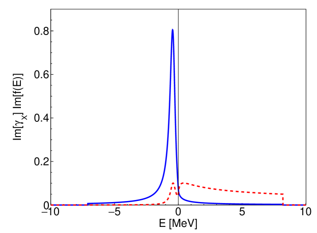
Figure 3: Line shapes in the SDD channel (solid blue curve) and in the CD channel (dashed red curve) for a bound state. The parameters are $\mathrm{Re}[\gamma_{X}]=+4\,\mathrm{Im}[\gamma_{X}]$ and $\mathrm{Im}[\gamma_{X}]=\sqrt{\mu\Gamma_{*0}}$. The branching fraction of the resonance feature into the SDD channel inferred from Eq. (37) is 0.52. The branching fraction of the bound state into the SDD channel inferred from Eq. (38) is 8/9.

In the limit $\mathrm{Re}[\gamma_{X}]^{2}\gg\mu\Gamma_{*0}$ with $\mathrm{Re}[\gamma_{X}]>0$, the positive sign of $\mathrm{Re}[\gamma_{X}]$ implies that the resonance is a bound state. The pole energy in Eq. (11) indicates that its binding energy is approximately $\mathrm{Re}[\gamma_{X}]^{2}/2\mu$. The position of a bound-state pole could be at the incoming arrow in Fig. 2, which is on the physical sheet of the complex energy plane. The line shapes in the SDD and CD channels for a bound-state resonance are illustrated in Fig. 3.

The SDD line shape is $\mathrm{Im}[\gamma_{X}]\,|f(E)|^{2}$, where the resonance factor is Eq. (16). Its properties can be expanded in powers of $1/\mathrm{Re}[\gamma_{X}]$. The maximum value of the line shape is $1/\mathrm{Im}[\gamma_{X}]$, up to a correction of order $1/\mathrm{Re}[\gamma_{X}]$. The maximum is at the energy

$$E_{\mathrm{SDD}}=-\frac{\mathrm{Re}[\gamma_{X}]^{2}}{2\mu}-\frac{\mathrm{Im}[\gamma_{X}]\,\Gamma_{*0}}{2\,\mathrm{Re}[\gamma_{X}]}+\ldots.$$ (17)

The energies where the line shape decreases to half the maximum value are lower by $\Gamma_{-}$ and higher by $\Gamma_{+}$, where

$$\Gamma_{-} = \frac{1}{2}\Gamma_{*0}+\frac{2\,\mathrm{Re}[\gamma_{X}]\,\mathrm{Im}[\gamma_{X}]+\mathrm{Im}[\gamma_{X}]^{2}}{2\mu},$$ (18a)

$$\Gamma_{+} = \frac{1}{2}\Gamma_{*0}+\frac{2\,\mathrm{Re}[\gamma_{X}]\,\mathrm{Im}[\gamma_{X}]-\mathrm{Im}[\gamma_{X}]^{2}}{2\mu},$$ (18b)

up to corrections of order $1/\mathrm{Re}[\gamma_{X}]$. The full width in the energy $E$ at half maximum is

$$\Gamma_{X}=\Gamma_{*0}+\frac{2\,\mathrm{Re}[\gamma_{X}]\,\mathrm{Im}[\gamma_{X}]}{\mu},$$ (19)

up to a correction of order $1/\mathrm{Re}[\gamma_{X}]^{5}$. This width $\Gamma_{X}$ coincides with the imaginary part of $-2E_{\mathrm{pole}}$, where the pole energy is given in Eq. (11). It can be interpreted as the decay rate of the bound state. The first term on the right side of Eq. (19) is the decay rate of the constituent $D^{*0}$ or $\bar{D}^{*0}$. The second term can be interpreted as the sum of the partial decay rates into short-distance decay modes. Given our assumption that $\mathrm{Im}[\gamma_{X}]$ is order $\sqrt{\mu\Gamma_{*0}}$, $\Gamma_{X}$ is much larger than $\Gamma_{*0}$ in the bound-state limit.

The CD line shape is $|f(E)|^{2}$ multiplied by the function of $E$ raised to the power $\tfrac{1}{2}$ in Eq. (13). This line shape has two local maxima: a bound-state peak below the threshold and a resonance enhancement above the threshold. The maximum of the bound-state peak in the CD channel is at the energy

$$E_{\mathrm{CD}}\approx-\frac{\mathrm{Re}[\gamma_{X}]^{2}-\mathrm{Im}[\gamma_{X}]^{2}}{2\mu},$$ (20)

up to a correction of order $1/\mathrm{Re}[\gamma_{X}]^{2}$. The maximum value of the peak differs from that in the SDD channel by a factor of $\mu\Gamma_{*0}/(2\,\mathrm{Re}[\gamma_{X}]\,\mathrm{Im}[\gamma_{X}])$, up to a relative correction of order $1/\mathrm{Re}[\gamma_{X}]^{2}$. The energies where the line shape decreases to half the maximum value are lower by $\Gamma_{X}/2$ and higher by $\Gamma_{X}/2$, up to corrections of order $1/\mathrm{Re}[\gamma_{X}]$. Thus the full width in the energy $E$ at half maximum is essentially the same as that for the SDD line shape in Eq. (19). The ratio of the integrals over $E$ of the bound-state peaks in the SDD and CD channels is therefore roughly equal to the ratio of their maximum values, which coincides with the ratio of the second and first terms in the expression for the width $\Gamma_{X}$ in Eq. (19). The SDD over CD branching ratio for the bound state is therefore large in the bound-state limit.

The second peak in the CD line shape comes from the threshold enhancement. Its maximum is at an energy near $+\mathrm{Re}[\gamma_{X}]^{2}/2\mu$ and its full width in $E$ at half maximum is approximately $4\sqrt{3}\,\mathrm{Re}[\gamma_{X}]^{2}/\mu$. The ratio of the heights of the peaks from the threshold enhancement and the bound state is approximately $\mathrm{Im}[\gamma_{X}]^{2}/\mu\Gamma_{*0}$. In Fig. 2, the choice $\mathrm{Im}[\gamma_{X}]=\sqrt{\mu\Gamma_{*0}}$ ensures that the two peaks have approximately the same height.

The resonance factor in Eq. (16) can be approximated by a Breit-Wigner function of $\sqrt{|E|}$ below the threshold and by a Lorentzian function of $\sqrt{E}$ above the threshold:

$$\big{|}f(E)\big{|}^{2} \approx \frac{1}{\big{(}\sqrt{2\mu|E|}-\mathrm{Re}[\gamma_{X}]\big{)}^{2}+\big{(}\mu\Gamma_{X}/2\,\mathrm{Re}[\gamma_{X}]\big{)}^{2}}\qquad E<0,$$ (21a)

$$\approx \frac{1}{\mathrm{Re}[\gamma_{X}]^{2}+\big{(}\sqrt{2\mu E}+\mu\Gamma_{X}/2\,\mathrm{Re}[\gamma_{X}]\big{)}^{2}}\qquad~{}~{}~{}~{}~{}\,E>0.$$ (21b)

The denominator of the Breit-Wigner function in Eq. (21a) has errors of order $1/\mathrm{Re}[\gamma_{X}]$ for negative $E$ of order $\mathrm{Re}[\gamma_{X}]^{2}/\mu$. It implies that the bound state has binding energy $\mathrm{Re}[\gamma_{X}]^{2}/2\mu$ and that its full width in $E$ at half maximum is $\Gamma_{X}$ in Eq. (19). The denominator of the Lorentzian function in Eq. (21b) has errors that are zeroth order in $\mathrm{Re}[\gamma_{X}]$ for positive $E$ of order $\mathrm{Re}[\gamma_{X}]^{2}/\mu$. The pole approximation in Eq. (12) gives a good approximation to the resonance factor $|f(E)|^{2}$ at real energies $E$ near the bound-state peak. It predicts the maximum and the energy at the maximum with relative errors of order $1/\mathrm{Re}[\gamma_{X}]^{2}$, and it predicts the full width at half maximum with a relative error of order $1/\mathrm{Re}[\gamma_{X}]^{5}$.

The resonance energy defined by Eq. (15) can be calculated using the approximation for $|f(E)|^{2}$ in Eq. (21) and then expanded in powers of $\Gamma_{X}$. The resonance energy is

$$E_{X}\approx-\frac{\mathrm{Re}[\gamma_{X}]^{2}}{2\mu}+\left[\log\frac{E_{\mathrm{max}}}{|E_{\mathrm{min}}|}-4\log\frac{2\,\mathrm{Re}[\gamma_{X}]^{2}}{\mu\Gamma_{X}}-2\right]\frac{\mu\Gamma_{X}^{2}}{16\,\mathrm{Re}[\gamma_{X}]^{2}}+\ldots.$$ (22)

We have simplified the coefficient of the leading correction term by taking the limit $|E_{\mathrm{min}}|\gg\mathrm{Re}[\gamma_{X}]^{2}/\mu$. The coefficient depends logarithmically on $E_{\mathrm{max}}/|E_{\mathrm{min}}|$ and on $\mathrm{Re}[\gamma_{X}]^{2}/\mu\Gamma_{X}$.

IV.2 Zero-energy resonance

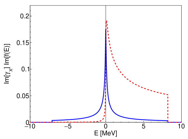
Figure 4: Line shapes in the SDD channel (solid blue curve) and in the CD channel (dashed red curve) for a zero-energy resonance. The parameters are $\mathrm{Re}[\gamma_{X}]=-\mathrm{Im}[\gamma_{X}]$ and $\mathrm{Im}[\gamma_{X}]=\sqrt{\mu\Gamma_{*0}}$. The branching fraction of the resonance feature into the SDD channel inferred from Eq. (37) is 0.22.

In the case $\mathrm{Re}[\gamma_{X}]=-\mathrm{Im}[\gamma_{X}]$, the negative sign of $\mathrm{Re}[\gamma_{X}]$ implies that the resonance is a virtual state. The pole energy in Eq. (11) indicates that the complex energy of the virtual state is order $\Gamma_{*0}$. The pole is on the second sheet of the complex energy plane, as illustrated in Fig. 2. The line shapes in the SDD and CD channels for a zero-energy resonance are illustrated in Fig. 4.

The resonance factor in Eq. (16) is an even function of $E$ whose maximum is at $E=0$. The maximum value is

$$\big{|}f(0)\big{|}^{2}=\frac{2}{\big{[}2\,\mathrm{Im}[\gamma_{X}]+\sqrt{2\mu\Gamma_{*0}}\,\big{]}^{2}}.$$ (23)

The full width in $E$ at half maximum is order $\Gamma_{*0}$. It changes smoothly from $1.73~{}\Gamma_{*0}$ if $\mathrm{Im}[\gamma_{X}]\ll\sqrt{\mu\Gamma_{*0}}$ to $3.75~{}\Gamma_{*0}$ if $\mathrm{Im}[\gamma_{X}]=\sqrt{\mu\Gamma_{*0}/2}$ to $0.54~{}\mathrm{Im}[\gamma_{X}]^{2}/\mu$ if $\mathrm{Im}[\gamma_{X}]\gg\sqrt{\mu\Gamma_{*0}}$. The pole approximation in Eq. (12) predicts correctly that the maximum of $|f(E)|^{2}$ is at $E=0$, but it does not a good approximation to the shape of the peak. It predicts, for example, that for $\mathrm{Im}[\gamma_{X}]=\sqrt{\mu\Gamma_{*0}/2}$, the maximum value is $\infty$ and the full width at half maximum is 0.

We can deduce an expression for the resonance energy $E_{X}$ by exploiting the fact that $f(E)$ is an even function of $E$, which implies that integrals of $|f(E)|^{2}$ satisfy

$$\int_{-E_{0}}^{0}\!dE\,\big{|}f(E)\big{|}^{2}=\int_{0}^{E_{0}}\!dE\,\big{|}f(E)\big{|}^{2}$$ (24)

for any $E_{0}$. By assuming $|E_{X}|\ll\Gamma_{*0}$ and using Eq. (24) with $E_{0}=|E_{\mathrm{min}}|$, we can reduce Eq. (15) for $E_{X}$ to an integral over the small-$E$ region where $|f(E)|^{2}$ reduces to $|f(0)|^{2}$ and an integral over the large-$E$ region where $|f(E)|^{2}$ reduces to $1/(2|E|)$. The resulting approximation for the resonance energy is

$$E_{X}\approx\left(\log\frac{E_{\mathrm{max}}}{|E_{\mathrm{min}}|}\right)\frac{\big{(}2\,\mathrm{Im}[\gamma_{X}]+\sqrt{2\mu\Gamma_{*0}}\,\big{)}^{2}}{8\mu}.$$ (25)

This result is valid provided the logarithm is small compared to 1, so that $|E_{X}|\ll\Gamma_{*0}$. This expression for $E_{X}$ can be positive or negative depending on whether $E_{\mathrm{max}}$ is larger or smaller than $|E_{\mathrm{min}}|$.

IV.3 Virtual-state limit

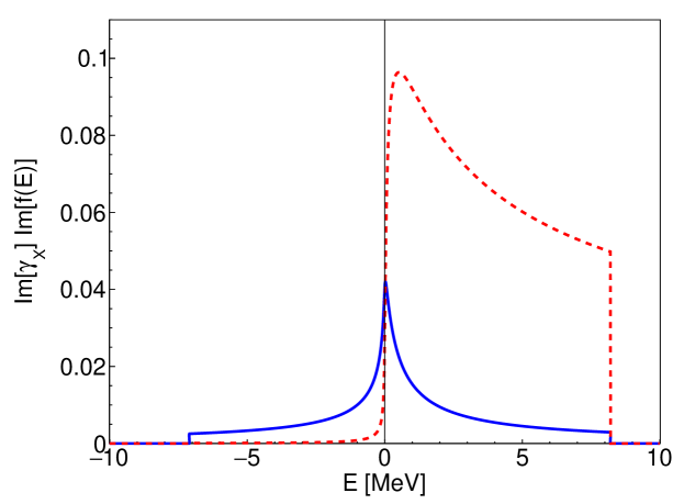
Figure 5: Line shapes in the SDD channel (solid blue curve) and in the CD channel (dashed red curve) for a virtual state. The parameters are $\mathrm{Re}[\gamma_{X}]=-4\,\mathrm{Im}[\gamma_{X}]$ and $\mathrm{Im}[\gamma_{X}]=\sqrt{\mu\Gamma_{*0}}$. The branching fraction of the resonance feature into the SDD channel inferred from Eq. (37) is 0.17.

In the limit $\mathrm{Re}[\gamma_{X}]^{2}\gg\mu\Gamma_{*0}$ with $\mathrm{Re}[\gamma_{X}]<0$, the negative sign of $\mathrm{Re}[\gamma_{X}]$ implies that the resonance is associated with a virtual state. The pole energy in Eq. (11) indicates that the virtual state has a negative energy that is approximately $-\mathrm{Re}[\gamma_{X}]^{2}/2\mu$. However the resonance energy $E_{X}$, which is also of order $\mathrm{Re}[\gamma_{X}]^{2}/\mu$, is positive. The position of a virtual-state pole could be at the outgoing arrow in Fig. 2, which is on the second sheet of the complex energy plane. The line shapes in the SDD and CD channels for a virtual-state resonance are illustrated in Fig. 5.

The resonance factor in Eq. (16) can be simplified by setting $\Gamma_{*0}=0$ and $\mathrm{Im}[\gamma_{X}]=0$:

$$\big{|}f(E)\big{|}^{2} \approx \frac{1}{\big{(}\sqrt{2\mu|E|}+\big{|}\mathrm{Re}[\gamma_{X}]\big{|}\big{)}^{2}}\qquad E<0,$$ (26a)

$$\approx \frac{1}{\mathrm{Re}[\gamma_{X}]^{2}+2\mu E}\qquad\qquad~{}~{}~{}~{}E>0.$$ (26b)

Its maximum is at $E=0$. It decreases to half the maximum at the energies $-0.086~{}\mathrm{Re}[\gamma_{X}]^{2}/\mu$ and $+\mathrm{Re}[\gamma_{X}]^{2}/2\mu$, so its full width at half maximum is $0.586~{}\mathrm{Re}[\gamma_{X}]^{2}/\mu$. The pole approximation in Eq. (12) gives a very bad approximation to the resonance factor $|f(E)|^{2}$ at real energies $E$. It predicts a maximum at an energy near $-\mathrm{Re}[\gamma_{X}]^{2}/2\mu$ instead of at 0.

The resonance energy defined by Eq. (15) can be obtained by evaluating integrals of the resonance factor in Eq. (26). Assuming $|E_{\mathrm{min}}|,E_{\mathrm{max}}\gg\mathrm{Re}[\gamma_{X}]^{2}/\mu$, the resonance energy can be approximated by

$$E_{X}\approx\left(e\,\sqrt{\frac{E_{\mathrm{max}}}{|E_{\mathrm{min}}|}}-1\right)\frac{\mathrm{Re}[\gamma_{X}]^{2}}{2\mu}.$$ (27)

This expression for $E_{X}$ is positive provided $E_{\mathrm{max}}>0.141\,|E_{\mathrm{min}}|$.

V Branching fractions

The difference between the line shapes of a near-threshold S-wave resonance and that of a conventional resonance complicates the definition of the $X$ branching fractions. In this Section, we emphasize the difference between branching fractions for an $X$ resonance feature and branching fractions for the $X$ bound state.

V.1 Branching fractions for the $\bm{X}$ resonance feature

The BaBar collaboration has recently determined the inclusive branching fraction of the $B^{+}$ meson into $K^{+}$ plus the $X$ resonance by measuring the recoil momentum spectrum of the $K^{+}$ Wormser . There is a peak in the momentum spectrum that corresponds to the recoil of the $K^{+}$ against a system with invariant mass near 3872 MeV. The recoiling system includes the threshold enhancement in $D^{*0}\bar{D}^{0}$ and $D^{0}\bar{D}^{*0}$ above the threshold as well as the decay products of a possible $X$ bound state below the threshold or a virtual state. We refer to the entire recoiling system as the $X$ resonance feature from $B^{+}\to K^{+}$ transitions, and we denote it by $X_{B^{+}\to K^{+}}$. The preliminary result for the inclusive branching fraction into the $X$ resonance feature, with errors combined in quadrature, is Wormser

$$\mathrm{Br}[B^{+}\to K^{+}X_{B^{+}\to K^{+}}]=(2.1\pm 0.7)\times 10^{-4}.$$ (28)

This result is consistent with previous upper bounds by the BaBar collaboration Aubert:2005vi and by the Belle collaboration Kato:2017gfv . If the measured product branching fraction for $B^{+}\to K^{+}(J/\psi\,\pi^{+}\pi^{-})$ Tanabashi:2018oca is divided by the inclusive branching fraction in Eq. (28), it gives Wormser

$$\mathrm{Br}[X_{B^{+}\to K^{+}}\to J/\psi\,\pi^{+}\pi^{-}]\equiv\frac{\mathrm{Br}[B^{+}\to K^{+}X]\,\mathrm{Br}[X\to J/\psi\,\pi^{+}\pi^{-}]}{\mathrm{Br}[B^{+}\to K^{+}X_{B^{+}\to K^{+}}]}=(4.1\pm 1.3)\%.$$ (29)

We refer to this as the $J/\psi\,\pi^{+}\pi^{-}$ branching fraction of the $X$ resonance feature from $B^{+}$-to-$K^{+}$ transitions. This branching fraction need not be the same for other production mechanisms, such as $B^{0}$-to-$K^{0}$ transitions or $e^{+}e^{-}$-to-$\gamma$ transitions.

If the resonance is associated with a bound state, the branching fraction of the $X$ resonance feature in Eq. (29) should be distinguished from the $J/\psi\,\pi^{+}\pi^{-}$ branching fraction of the $X$ bound state, which we denote by $\mathrm{Br}[X\to J/\psi\,\pi^{+}\pi^{-}]$ with no subscript on $X$. This larger branching fraction could be obtained by dividing the product branching fraction for $B^{+}\to K^{+}(J/\psi\,\pi^{+}\pi^{-})$ by the branching fraction of $B^{+}$ into $K^{+}$ plus the $X$ bound state, which we denote by $\mathrm{Br}[B^{+}\to K^{+}X]$ with no subscript on $X$. This branching fraction into the $X$ bound state has not been measured. The branching fractions of the $X$ bound state should be the same for all short-distance production mechanisms, because they can be obtained by factoring the production amplitudes at the bound-state pole as in Eq. (6).

The $D^{0}\bar{D}^{0}\pi^{0}$ branching fraction of the $X$ resonance feature from $B^{+}$-to-$K^{+}$ transitions can be obtained using measurements by the Belle collaboration of the decay $B^{+}\to K^{+}(D^{0}\bar{D}^{0}\pi^{0})$ Gokhroo:2006bt . The $D^{0}\bar{D}^{0}\pi^{0}$ invariant mass distribution has a narrow peak near the $D^{*0}\bar{D}^{0}$ threshold that can be identified with the $X$ resonance feature. The measured branching fraction for events in the peak can be interpreted as the contribution to the inclusive branching fraction into the $X$ resonance feature in Eq. (28) from the final state $D^{0}\bar{D}^{0}\pi^{0}$. Dividing by that inclusive branching fraction, we obtain the $D^{0}\bar{D}^{0}\pi^{0}$ branching fraction of the $X$ resonance feature from $B^{+}$-to-$K^{+}$ transitions:

$$\mathrm{Br}[X_{B^{+}\to K^{+}}\to D^{0}\bar{D}^{0}\pi^{0}]\equiv\frac{\mathrm{Br}[B^{+}\to K^{+}(D^{0}\bar{D}^{0}\pi^{0})]}{\mathrm{Br}[B^{+}\to K^{+}X_{B^{+}\to K^{+}}]}=(49\pm 26)\%,$$ (30)

where we have combined the errors in quadrature. The CD branching fraction is the sum of the branching fractions into $D^{0}\bar{D}^{0}\pi^{0}$ and $D^{0}\bar{D}^{0}\gamma$. The additional contribution from the final state $D^{0}\bar{D}^{0}\gamma$ can be taken into account approximately by dividing the branching fraction in Eq. (30) by the known branching fraction of $D^{*0}$ into $D^{0}\pi^{0}$. The resulting estimate for the CD branching fraction of the $X$ resonance feature from $B^{+}$-to-$K^{+}$ transitions is

$$\mathrm{Br}[X_{B^{+}\to K^{+}}\to D^{0}\bar{D}^{0}(\pi^{0},\gamma)]\approx\frac{\mathrm{Br}[X_{B^{+}\to K^{+}}\to D^{0}\bar{D}^{0}\pi^{0}]}{\mathrm{Br}[D^{*0}\to D^{0}\pi^{0}]}=(75\pm 40)\%.$$ (31)

The corresponding estimate for the SDD branching fraction is the complimentary fraction $(25\pm 40)\%$.

Assuming decays of the $X$ resonance feature into $J/\psi\,\pi^{+}\pi^{-}$ are dominated by decays of the $X$ bound state, we can obtain an estimate of the $D^{0}\bar{D}^{0}(\pi^{0},\gamma)$ over $J/\psi\,\pi^{+}\pi^{-}$ branching ratio for the $X$ resonance feature from $B^{+}$-to-$K^{+}$ transitions by dividing the Belle result for the product branching fraction for $B^{+}\to K^{+}(D^{0}\bar{D}^{0}\pi^{0})$ Gokhroo:2006bt by the measured product branching fraction for $B^{+}\to K^{+}(J/\psi\,\pi^{+}\pi^{-})$ Tanabashi:2018oca and by the branching fraction for $D^{*0}\to D^{0}\pi^{0}$:

$$\frac{\mathrm{Br}[X_{B^{+}\to K^{+}}\to D^{0}\bar{D}^{0}(\pi^{0},\gamma)]}{\mathrm{Br}[X_{B^{+}\to K^{+}}\to J/\psi\,\pi^{+}\pi^{-}]}=18.3\pm 7.8.$$ (32)

Estimates of the CD branching fraction of the $X$ resonance feature from $B^{+}$-to-$K^{+}$ transitions can also be obtained from measurements by the BaBar and Belle collaborations of the decays of $B^{+}$ into $K^{+}$ plus $D^{*0}\bar{D}^{0}$ Aubert:2007rva ; Adachi:2008sua . These measurements are complicated by systematic errors associated with constraining the momenta of $D^{0}$ and $\pi^{0}$ with invariant mass close to the mass of the $D^{*0}$ so their invariant mass is exactly $M_{*0}$ Stapleton:2009ey . This procedure moves $D^{0}\bar{D}^{0}\pi^{0}$ events with invariant mass below the $D^{*0}\bar{D}^{0}$ threshold to above the threshold. The resulting measurement of the resonance energy of the $X$ in the $D^{0}\bar{D}^{*0}$ decay mode therefore has an undetermined positive systematic error Stapleton:2009ey . The complications from constraining momenta so the invariant mass of $D^{0}\pi^{0}$ or $\bar{D}^{0}\pi^{0}$ is $M_{*0}$ affects a measurement of the energy and width of the resonance more than a measurement of the branching fraction. We can therefore interpret a measured product branching fraction for the decay $B^{+}\to K^{+}\,(D^{*0}\bar{D}^{0},D^{0}\bar{D}^{*0})$ as an approximation to that for the decay $B^{+}\to K^{+}\,D^{0}\bar{D}^{0}(\pi^{0},\gamma)$. A branching fraction for the $X$ resonance feature into $D^{0}\bar{D}^{0}(\pi^{0},\gamma)$ can then be obtained by dividing the measured product branching fraction by the inclusive branching fraction in Eq. (28). The BaBar measurement in Ref. Aubert:2007rva gives the estimate $(80\pm 38)\%$, which is consistent with the branching fraction in Eq. (31). The Belle measurement in Ref. Adachi:2008sua gives the estimate $(37\pm 15)\%$, whose central value is significantly smaller than that in Eq. (31).

V.2 Branching fractions for the $\bm{X}$ bound state

If $X$ is a narrow bound state whose width is sufficiently small compared to its binding energy, it has well-defined branching fractions into its various decay modes that do not depend on the production mechanism. The branching fractions into short-distance decay modes should be considerably larger than the corresponding branching fractions for an $X$ resonance feature. The $J/\psi\,\pi^{+}\pi^{-}$ branching fraction of the $X$ resonance feature from $B^{+}$-to-$K^{+}$ transitions in Eq. (29) can be taken as a loose lower bound on the $J/\psi\,\pi^{+}\pi^{-}$ branching fraction for the $X$ bound state. An upper bound on the $J/\psi\,\pi^{+}\pi^{-}$ branching fraction for the $X$ bound state can be obtained from measurements of branching ratios for other decay modes. The bound is obtained most easily by using the equality

$$\frac{1}{\mathrm{Br}[X\to J/\psi\,\pi^{+}\pi^{-}]}=1+{\sum_{i}}^{\prime}\frac{\mathrm{Br}[X\to i]}{\mathrm{Br}[X\to J/\psi\,\pi^{+}\pi^{-}]}+\frac{\mathrm{Br}[X\to D^{0}\bar{D}^{0}(\pi^{0},\gamma)]}{\mathrm{Br}[X\to J/\psi\,\pi^{+}\pi^{-}]},$$ (33)

where the sum over $i$ is over SDD modes other than $J/\psi\,\pi^{+}\pi^{-}$. The other SDD modes that have been observed are $J/\psi\,\pi^{+}\pi^{-}\pi^{0}$, $J/\psi\,\gamma$, $\psi(2S)\,\gamma$, and $\chi_{c1}\,\pi^{0}$. The branching ratio on the right side of Eq. (33) for $i=J/\psi\,\pi^{+}\pi^{-}\pi^{0}$ (which is often called $J/\psi\,\omega$) is $0.8\pm 0.3$ delAmoSanchez:2010jr . The branching ratio for $i=J/\psi\,\gamma$ is determined to be $0.24\pm 0.05$ by calculating the ratio of product branching fractions from $B^{+}\to K^{+}X$ decays Tanabashi:2018oca . The branching ratio for $i=\psi(2S)\,\gamma$ can be obtained from that for $J/\psi\,\gamma$ by multiplying by the branching ratio $2.6\pm 0.6$ for the decays of $X$ into $\psi(2S)\,\gamma$ over $J/\psi\,\gamma$ Tanabashi:2018oca . The branching ratio for the recently observed decay mode $i=\chi_{c1}\,\pi^{0}$ is $0.88\pm 0.34$ Ablikim:2019soz . With these four decay modes included but the last term in Eq. (33) excluded, the right side of Eq. (33) is $3.56\pm 0.51$. Its reciprocal is $(28.1\pm 4.1)\%$. An upper bound on the branching fraction with 90% confidence level can be obtained by adding $1.28\,\sigma$ to the central value:

$$\mathrm{Br}[X\to J/\psi\,\pi^{+}\pi^{-}]<33\%\qquad(90\%~{}\mathrm{C.L.}).$$ (34)

This upper bound would be 44% if the decay mode $\chi_{c1}\,\pi^{0}$ was not taken into account. The $D^{0}\bar{D}^{0}(\pi^{0},\gamma)$ term in Eq. (33) cannot be taken into account, because there are no measurements of this branching ratio for the $X$ bound state.

The identity in Eq. (33) holds equally well if all the branching fractions for the $X$ bound state are replaced by branching fractions for an $X$ resonance feature. We can use this identity to obtain an upper bound on the $J/\psi\,\pi^{+}\pi^{-}$ branching fraction of the $X$ resonance feature from $B^{+}$-to-$K^{+}$ transitions. We assume the branching ratio of the $X$ resonance feature for each SDD mode $i$ over $J/\psi\,\pi^{+}\pi^{-}$ is the same as the corresponding branching ratio of the $X$ bound state. An estimate for the $D^{0}\bar{D}^{0}(\pi^{0},\gamma)$ over $J/\psi\,\pi^{+}\pi^{-}$ branching ratio for the $X$ resonance feature from $B^{+}$-to-$K^{+}$ transitions is given in Eq. (32). If the last term in Eq. (33) is replaced by this value, the right side becomes $21.9\pm 7.8$. Its reciprocal is $(4.6\pm 1.6)\%$. An upper bound with 90% confidence level on the $J/\psi\,\pi^{+}\pi^{-}$ branching fraction of the $X$ resonance feature from $B^{+}$-to-$K^{+}$ transitions can be obtained by adding $1.28\,\sigma$ to the central value:

$$\mathrm{Br}[X_{B^{+}\to K^{+}}\to J/\psi\,\pi^{+}\pi^{-}]<6.7\%\qquad(90\%~{}\mathrm{C.L.}).$$ (35)

This upper bound is consistent with the branching fraction in Eq. (29) determined recently by the BaBar collaboration Wormser .

Upper bounds on the branching fraction for $X$ into $J/\psi\,\pi^{+}\pi^{-}$ that are significantly smaller than that in Eq. (34) have been derived previously, but they are actually upper bounds on the branching fraction for an $X$ resonance feature into $J/\psi\,\pi^{+}\pi^{-}$. The upper bound without taking into account the decay mode $\chi_{c1}\,\pi^{0}$ was given as 8.3% in Ref. Guo:2014sca and 10% in Ref. Yuan:2018inv . These are much smaller than our upper bound of 44% without taking into account $\chi_{c1}\,\pi^{0}$. A smaller upper bound can be obtained by approximating the last term in Eq. (33) by the ratio $9.9\pm 3.2$ of the PDG values for the product branching fractions for $B^{+}\to K^{+}(\bar{D}^{*0}D^{0})$ and $B^{+}\to K^{+}(J/\psi\,\pi^{+}\pi^{-})$ Tanabashi:2018oca . With this additional contribution to the right side of Eq. (33) but with the $\chi_{c1}\,\pi^{0}$ term excluded, it becomes $12.6\pm 3.2$. Its reciprocal is $(8.0\pm 2.0)\%$. The central value is consistent with the upper bound in Ref. Guo:2014sca . Adding $1.28\,\sigma$ to the central value to get an upper bound at the 90% confidence level gives 10.5%, which is close to the upper bound in Ref. Yuan:2018inv . Having used a product branching fraction for $B^{+}\to K^{+}(\bar{D}^{*0}D^{0})$ as an input, the upper bounds in Refs. Guo:2014sca and Yuan:2018inv are actually on the $J/\psi\,\pi^{+}\pi^{-}$ branching fraction of the $X$ resonance feature from $B^{+}$-to-$K^{+}$ transitions.

V.3 Theoretical branching fractions

Because the $X$ line shapes differ from those of a conventional resonance, theoretical expressions for the branching fractions of the $X$ resonance require a prescription. The branching ratio of a resonance feature into the final state $k$ over the final state $l$ can be expressed as a ratio of integrals of the corresponding contributions to the inclusive line shape, which has the form in Eq. (5):

$$\frac{\mathrm{Br}[X_{\mathrm{res}}\to k]}{\mathrm{Br}[X_{\mathrm{res}}\to l]}=\frac{\sum_{ij}B_{i}{B_{j}}^{*}\int_{E_{\mathrm{min}}}^{E_{\mathrm{max}}}\!dE\,\mathrm{Im}[f_{ij}(E)]^{(k)}}{\sum_{ij}B_{i}{B_{j}}^{*}\int_{E_{\mathrm{min}}}^{E_{\mathrm{max}}}\!dE\,\mathrm{Im}[f_{ij}(E)]^{(l)}}.$$ (36)

We have used the simple prescription for the resonance as the energy range between the specified energies $E_{\mathrm{min}}$ below the scattering threshold and $E_{\mathrm{max}}$ above the threshold. An alternative prescription would be to weight the integrals in Eq. (36) by a Gaussian function of $E$ and extend the limits of the integrals to $-\infty$ and $+\infty$. The choice of the resonance feature, which is represented by $X_{\mathrm{res}}$, determines the short-distance coefficients $B_{i}$.

In the simplest model for the $X$ line shapes, there is a single resonant scattering channel with the scattering amplitude $f(E)$ in Eq. (10). The inclusive line shape is proportional to the function $\mathrm{Im}[f(E)]$ in Eq. (13). The SDD over CD branching ratio of the $X$ resonance feature can be expressed as a ratio of integrals:

$$\frac{\mathrm{Br}[X_{\mathrm{res}}\to\mathrm{SDD}]}{\mathrm{Br}[X_{\mathrm{res}}\to D^{0}\bar{D}^{0}(\pi^{0},\gamma)]}=\frac{\mathrm{Im}[\gamma_{X}]\,\int_{E_{\mathrm{min}}}^{E_{\mathrm{max}}}\!dE\,\big{|}f(E)\big{|}^{2}}{\int_{E_{\mathrm{min}}}^{E_{\mathrm{max}}}\!dE\,\big{|}f(E)\big{|}^{2}\big{[}\mu\sqrt{E^{2}+\Gamma_{*0}^{2}/4}+\mu E\big{]}^{1/2}}.$$ (37)

The numerator depends logarithmically on $E_{\mathrm{min}}$ and $E_{\mathrm{max}}$. The denominator is insensitive to $E_{\mathrm{min}}$, but it depends on the upper endpoint as $E_{\mathrm{max}}^{1/2}$. The integrals in Eq. (37) are complicated functions of $\Gamma_{*0}$ and the real and imaginary parts of $\gamma_{X}$. Given an SDD over CD branching ratio BR, such as that in Eq. (37), the SDD branching fraction is $\mathrm{BF}=\mathrm{BR}/(1+\mathrm{BR})$.

If the $X$ is a narrow bound state whose width is sufficiently small compared to its binding energy, the branching fractions for decays of the bound state are well defined and they do not depend on the production mechanism. They give the fractions of events that would be observed if the energy $E$ could be tuned to closer to the negative resonance energy $E_{X}$ than the half-width $\Gamma_{X}/2$. In the simplest model for the $X$ line shapes, the SDD over CD branching ratio for the $X$ bound state can be approximated by the ratio of the two terms in the expression for $\Gamma_{X}$ in Eq. (19):

$$\frac{\mathrm{Br}[X\to\mathrm{SDD}]}{\mathrm{Br}[X\to D^{0}\bar{D}^{0}(\pi^{0},\gamma)]}\approx\frac{2\,\mathrm{Re}[\gamma_{X}]\,\mathrm{Im}[\gamma_{X}]}{\mu\Gamma_{*0}}.$$ (38)

This is a simple function of $\Gamma_{*0}$ and the real and imaginary parts of $\gamma_{X}$. This expression for the branching ratio has an unphysical negative value when $\mathrm{Re}[\gamma_{X}]$ is negative. It is therefore a reasonable approximation only $\mathrm{Re}[\gamma_{X}]$ is large enough, corresponding to a sufficiently narrow bound state. As a reasonable quantitative criterion for the validity of Eq. (38), we choose to require the real part of the pole energy $E_{\mathrm{pole}}$ in Eq. (11) to be larger in absolute value than its imaginary part. This criterion implies that the boundary of the region where the bound state is sufficiently narrow is when the real part of $\gamma_{X}$ is

$$\mathrm{Re}[\gamma_{X}]=\mathrm{Im}[\gamma_{X}]+\sqrt{2\,\mathrm{Im}[\gamma_{X}]^{2}+\mu\Gamma_{*0}}.$$ (39)

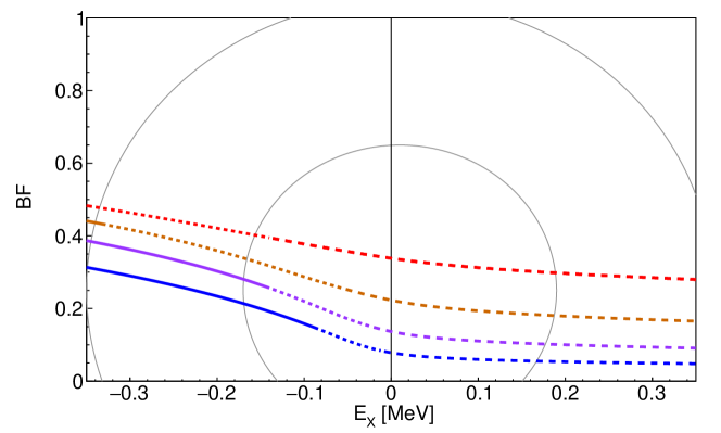
Figure 6: Branching fraction for short-distance decays of the $X$ resonance feature as a function of the resonance energy $E_{X}$ for four values of $\mathrm{Im}[\gamma_{X}]/\sqrt{\mu\Gamma_{*0}}$: 2, 1, 1/2, and 1/4 in order of decreasing branching fractions. The branching fraction implied by Eq. (37) is shown as a curve that changes from solid for a narrow bound state to dotted for a bound state that is not so narrow and then to dashed for a virtual state. The thin grey curves are the $1\sigma$ and $2\sigma$ error ellipses for $E_{X}$ in Eq. (7) and the complement $(25\pm 40)\%$ of the branching fraction in Eq. (31).

If $E_{\mathrm{min}}$ and $E_{\mathrm{max}}$ are specified, Eqs. (15) and (37) can be used to determine the two unknown parameters $\mathrm{Re}[\gamma_{X}]$ and $\mathrm{Im}[\gamma_{X}]$ given the measured value of the resonance energy $E_{X}$ in Eq. (7) and the estimate of the CD branching fraction for the $X$ resonance feature in Eq. (31). Alternatively, for a given value of $\mathrm{Im}[\gamma_{X}]$, Eq. (15) can be used to determine $\mathrm{Re}[\gamma_{X}]$ as a function of $E_{X}$. The SDD branching fraction BF for the $X$ resonance feature implied by Eq. (37) can then be predicted as a function of $E_{X}$. It can be compared to the estimated value $\mathrm{BF}=(25\pm 40)\%$ given by the complement of Eq. (31). In Fig. 6, the SDD branching fraction BF for the $X$ resonance feature is shown as a function of the resonance energy $E_{X}$ for various values of $\mathrm{Im}[\gamma_{X}]$. A curve changes from solid, indicating a narrow bound state, to dotted when $\mathrm{Re}[\gamma_{X}]$ decreases through the value in Eq. (39). The curve changes from dotted to dashed when $\mathrm{Re}[\gamma_{X}]$ becomes negative, indicating that the bound state has become a virtual state. The error ellipses in Fig. 6 are for the measured resonance energy $E_{X}$ in Eq. (7) and for the estimated branching fraction $\mathrm{BF}=(25\pm 40)\%$. The curves within the $1\sigma$ error ellipse are compatible with values of $\mathrm{Im}[\gamma_{X}]/\sqrt{\mu\Gamma_{*0}}$ up to about 9. The majority of the area inside the $1\sigma$ error ellipse corresponds to virtual states, but there is a region with negative $E_{X}$ that corresponds to narrow bound states.

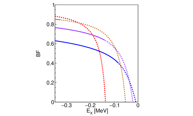
Figure 7: Branching fraction for short-distance decays of the $X$ bound state as a function of the resonance energy $E_{X}$ for four values of $\mathrm{Im}[\gamma_{X}]/\sqrt{\mu\Gamma_{*0}}$: 2, 1, 1/2, and 1/4 in order of decreasing branching fractions on the left side. The approximation for the branching fraction implied by Eq. (38) is shown as a curve that changes from solid for a narrow bound state to dotted when the bound state is not so narrow.

The approximation in Eq. (38) for the SDD over CD branching ratio of the $X$ bound state implies a corresponding approximation for the SDD branching fraction of the $X$ bound state. In Fig. 7, we show the SDD branching fraction of the $X$ bound state as a function of the resonance energy $E_{X}$ for various values of $\mathrm{Im}[\gamma_{X}]$. A curve changes from solid, indicating a narrow bound state, to dotted when $\mathrm{Re}[\gamma_{X}]$ decreases through the value in Eq. (39). The dotted curve decreases to zero when $\mathrm{Re}[\gamma_{X}]$ is 0, indicating that the bound state is about to become a virtual state. In most of the region that corresponds to narrow bound states, the branching fraction in Fig. 7 is considerably larger than the corresponding branching fraction for the $X$ resonance feature in Fig. 6. Within the $1\sigma$ error ellipse, the ratio of the branching fraction for the $X$ bound state over the $X$ resonance feature ranges from 2.5 to 3.2. The simplest model for the $X$ line shapes predicts that the $J/\psi\,\pi^{+}\pi^{-}$ branching fraction of a narrow bound state should be larger than that of the $X$ resonance feature in Eq. (29) by that same factor.

VI Summary

Preliminary measurements by the BaBar collaboration of the recoil momentum distribution of the $K^{+}$ in $B^{+}$ decays have been used to determine the $J/\psi\,\pi^{+}\pi^{-}$ branching fraction of the $X(3872)$ resonance feature from $B^{+}$-to-$K^{+}$ transitions in Eq. (29). We have emphasized that this is not a conventional branching fraction that must be independent of the production process. If $X$ is a narrow bound state, its branching fractions must be the same for all short-distance production mechanisms, because they can be obtained by factoring amplitudes at the pole associated with the bound state. However a branching fraction of the $X$ resonance feature is obtained by integrating over the energy of the resonance feature, which includes a threshold enhancement peak as well as a possible bound-state peak, and it should therefore be expected to depend on the production mechanism. We used a previous measurement by the Belle collaboration to obtain the $D^{0}\bar{D}^{0}\pi^{0}$ branching fraction of the $X$ resonance feature from $B^{+}$-to-$K^{+}$ transitions in Eq. (30). A more precise measurement of the $D^{0}\bar{D}^{0}\pi^{0}$ branching fraction of the $X$ resonance feature and a measurement of its $D^{0}\bar{D}^{0}\gamma$ branching fraction would be useful.

The current experimental result for the $X$ resonance energy $E_{X}$, which is obtained from measurements in the $J/\psi\,\pi^{+}\pi^{-}$ decay mode, is given in Eq. (7), and it is rather precise. We introduced a theoretical prescription for the $X$ resonance energy in Eq. (14) that can be useful for constraining the parameters of models for the $X$ line shapes. This prescription is just the center of energy in the $i=J/\psi\,\pi^{+}\pi^{-}$ decay mode. We illustrated it by applying it to the simplest plausible model for the $X$ line shapes, which can be specified by the scattering amplitude in Eq. (10) and by the energy range from $E_{\mathrm{min}}$ to $E_{\mathrm{max}}$. We derived analytic approximations for $E_{X}$ in three limits: the bound-state limit in Eq. (22), the zero-energy resonance in Eq. (25), and the virtual-state limit in Eq. (27).

Our estimate of the branching fraction into constituent decay modes of the $X$ resonance feature from $B^{+}$-to-$K^{+}$ transitions in Eq. (31) implies that the complementary branching fraction into short-distance decay modes is $\mathrm{BF}=(25\pm 40)\%$. Using the measured value of $E_{X}$ in Eq. (7) and our estimate of BF, we obtained constraints on the parameters of the simplest plausible model for the $X$ line shapes. Further measurements of branching fractions of $X$ resonance features could be used to determine the constraints on the parameters for more realistic models of the $X$ line shapes that explicitly take into account additional channels, such as the charged-charm-meson-pair channel or the $\chi_{c1}(2P)$ channel.

If the $X$ is a narrow bound state, the branching fraction of the $X$ bound state into a short-distance decay mode can be substantially larger than the corresponding branching fraction of the $X$ resonance feature. The $J/\psi\,\pi^{+}\pi^{-}$ branching fraction of the $X$ bound state can therefore be substantially larger than the $J/\psi\,\pi^{+}\pi^{-}$ branching fraction of the $X$ resonance feature. A loose lower bound on the $J/\psi\,\pi^{+}\pi^{-}$ branching fraction of the $X$ bound state is provided by the $J/\psi\,\pi^{+}\pi^{-}$ branching fraction of the $X$ resonance feature in Eq. (29). An upper bound on the $J/\psi\,\pi^{+}\pi^{-}$ branching fraction of the $X$ bound state is given in Eq. (34).

The $X$ can be produced by the creation of a $D^{*}\bar{D}^{*}$ pair at short distances followed by the rescattering of the charm mesons into $X\pi$ or $X\gamma$. A charm-meson triangle singularity produces a narrow peak in the invariant mass distribution for $X\pi$ or $X\gamma$ near the $D^{*}\bar{D}^{*}$ threshold Guo:2019qcn ; Braaten:2019gfj . Under the assumption that $X$ is a narrow bound state, we have calculated the production rate of $X\pi$ near the peak from the triangle singularity in hadron colliders Braaten:2018eov ; Braaten:2019gfj and in $B$ meson decay Braaten:2019yua . We also calculated the cross section for electron-positron annihilation into $X\gamma$ near the peak from the triangle singularity Braaten:2019gfj . For the coupling of the $X$ bound state to the charm-meson pairs, we used a vertex determined by the binding energy. The cross section for producing $X$ in the specific decay mode $J/\psi\,\pi^{+}\pi^{-}$ is obtained by multiplying the cross section for producing the $X$ bound state by the $J/\psi\,\pi^{+}\pi^{-}$ branching fraction for the $X$ bound state. That branching fraction should be considerably larger than the roughly 4% branching fraction of the $X$ resonance feature in Eq. (29), and it should be smaller than the upper bound of 33% in Eq. (34). Tighter constraints on this branching fraction would allow more precise predictions of the heights of the peaks from the triangle singularity observed through the $J/\psi\,\pi^{+}\pi^{-}$ decay mode of the $X$. The observation of these peaks would provide convincing evidence for the identification of the $X$ as a weakly-bound charm-meson molecule.

Note added: As this paper was being finalized, Li and Yuan posted a paper entitled “Determination of the absolute branching fractions of $X(3872)$ decays” Li:2019kpj . They presented a complete analysis of all the existing data that can give $X$ branching fractions. Their branching fractions should not be interpreted as those for the $X$ bound state, because their inputs included several results for $X$ resonance features from various production mechanisms. In addition to the inclusive branching fraction of $B^{+}$ into $K^{+}$ plus the $X$ resonance feature from Ref. Wormser , they included results for the $D^{*0}\bar{D}^{0}$ and $D^{0}\bar{D}^{*0}$ final states from the $X$ resonance feature from $B^{+}$-to-$K^{+}$ transitions, from $B^{0}$-to-$K^{0}$ transitions, and from $e^{+}e^{-}$-to-$\gamma$ transitions. Their analysis relied on the unjustified assumption that the branching fractions for $X$ resonance features are the same for these three production mechanisms.

- (1) H.X. Chen, W. Chen, X. Liu and S.L. Zhu, The hidden-charm pentaquark and tetraquark states, Phys. Rept. 639, 1 (2016) [arXiv:1601.02092].
- (2) A. Hosaka, T. Iijima, K. Miyabayashi, Y. Sakai and S. Yasui, Exotic hadrons with heavy flavors: , , , and related states, PTEP 2016, 062C01 (2016) [arXiv:1603.09229].
- (3) R.F. Lebed, R.E. Mitchell and E.S. Swanson, Heavy-Quark QCD Exotica, Prog. Part. Nucl. Phys. 93, 143 (2017) [arXiv:1610.04528].
- (4) A. Esposito, A. Pilloni and A.D. Polosa, Multiquark Resonances, Phys. Rept. 668, 1 (2016) [arXiv:1611.07920].
- (5) F.K. Guo, C. Hanhart, U.G. Meißner, Q. Wang, Q. Zhao and B.S. Zou, Hadronic molecules, Rev. Mod. Phys. 90, 015004 (2018) [arXiv:1705.00141].
- (6) A. Ali, J.S. Lange and S. Stone, Exotics: Heavy Pentaquarks and Tetraquarks, Prog. Part. Nucl. Phys. 97, 123 (2017) [arXiv:1706.00610].
- (7) S.L. Olsen, T. Skwarnicki and D. Zieminska, Nonstandard heavy mesons and baryons: Experimental evidence, Rev. Mod. Phys. 90, 015003 (2018) [arXiv:1708.04012].
- (8) M. Karliner, J.L. Rosner and T. Skwarnicki, Multiquark States, Ann. Rev. Nucl. Part. Sci. 68, 17 (2018) [arXiv:1711.10626].
- (9) C.Z. Yuan, The states revisited, Int. J. Mod. Phys. A 33, 1830018 (2018) [arXiv:1808.01570].
- (10) N. Brambilla, S. Eidelman, C. Hanhart, A. Nefediev, C.P. Shen, C.E. Thomas, A. Vairo and C.Z. Yuan, The states: experimental and theoretical status and perspectives, arXiv:1907.07583 [hep-ex].
- (11) S.K. Choi et al. [Belle Collaboration], Observation of a narrow charmonium-like state in exclusive decays, Phys. Rev. Lett. 91, 262001 (2003) [hep-ex/0309032].
- (12) R. Aaij et al. [LHCb Collaboration], Determination of the meson quantum numbers, Phys. Rev. Lett. 110, 222001 (2013) [arXiv:1302.6269].
- (13) M. Tanabashi et al. [Particle Data Group], Review of Particle Physics, Phys. Rev. D 98, 030001 (2018).
- (14) E. Braaten, L.-P. He and K. Ingles, Predictive Solution to the Collider Production Puzzle, arXiv:1811.08876 [hep-ph].
- (15) E. Braaten, L.-P. He and K. Ingles, Production of Accompanied by a Pion in Meson Decay, arXiv:1902.03259 [hep-ph].
- (16) E. Braaten, L.-P. He and K. Ingles, Production of Accompanied by a Pion at Hadron Colliders, arXiv:1903.04355 [hep-ph].
- (17) S. Dubynskiy and M.B. Voloshin, near the threshold, Phys. Rev. D 74, 094017 (2006) [hep-ph/0609302].
- (18) F.K. Guo, Novel method for precisely measuring the mass, Phys. Rev. Lett. 122, 202002 (2019) [arXiv:1902.11221].
- (19) E. Braaten, L.-P. He and K. Ingles, Triangle Singularity in the Production of and a Photon in Annihilation, arXiv:1904.12915 [hep-ph].
- (20) G. Wormser (on behalf of the BaBar collaboration), presented at Quarkonium 2019 in Torino, May 2019.
- (21) E. Braaten and H.-W. Hammer, Universality in few-body systems with large scattering length, Phys. Rept. 428, 259 (2006) [cond-mat/0410417].
- (22) J.L. Rosner, Hadronic and radiative widths, Phys. Rev. D 88, 034034 (2013) [arXiv:1307.2550].
- (23) G. Gokhroo et al. [Belle Collaboration], Observation of a Near-threshold Enhancement in Decay, Phys. Rev. Lett. 97, 162002 (2006) [hep-ex/0606055].
- (24) M.B. Voloshin, Interference and binding effects in decays of possible molecular component of , Phys. Lett. B 579, 316 (2004) [hep-ph/0309307].
- (25) M.B. Voloshin, Isospin properties of the state near the threshold, Phys. Rev. D 76, 014007 (2007) [arXiv:0704.3029].
- (26) E. Braaten and M. Lu, Line shapes of the , Phys. Rev. D 76, 094028 (2007) [arXiv:0709.2697].
- (27) C. Hanhart, Y.S. Kalashnikova, A.E. Kudryavtsev and A.V. Nefediev, Reconciling the with the near-threshold enhancement in the final state, Phys. Rev. D 76, 034007 (2007) [arXiv:0704.0605].
- (28) O. Zhang, C. Meng and H.Q. Zheng, Ambiversion of , Phys. Lett. B 680, 453 (2009) [arXiv:0901.1553].
- (29) Y.S. Kalashnikova and A.V. Nefediev, Nature of from data, Phys. Rev. D 80, 074004 (2009) [arXiv:0907.4901].
- (30) P. Artoisenet, E. Braaten and D. Kang, Using Line Shapes to Discriminate between Binding Mechanisms for the , Phys. Rev. D 82, 014013 (2010) [arXiv:1005.2167].
- (31) E. Braaten and M. Lu, The Effects of charged charm mesons on the line shapes of the , Phys. Rev. D 77, 014029 (2008) [arXiv:0710.5482].
- (32) C. Hanhart, Y.S. Kalashnikova and A.V. Nefediev, Interplay of quark and meson degrees of freedom in a near-threshold resonance: multi-channel case, Eur. Phys. J. A 47, 101 (2011) [arXiv:1106.1185].
- (33) X.W. Kang and J.A. Oller, Different pole structures in line shapes of the , Eur. Phys. J. C 77, 399 (2017) [arXiv:1612.08420].
- (34) E. Braaten and D. Kang, Decay Channel of the (3872) Charm Meson Molecule, Phys. Rev. D 88, no. 1, 014028 (2013) [arXiv:1305.5564].
- (35) S. Fleming, M. Kusunoki, T. Mehen and U. van Kolck, Pion interactions in the , Phys. Rev. D 76, 034006 (2007) [hep-ph/0703168].
- (36) E. Braaten, Galilean-invariant effective field theory for the , Phys. Rev. D 91, 114007 (2015) [arXiv:1503.04791].
- (37) V. Baru, A. A. Filin, C. Hanhart, Y.S. Kalashnikova, A.E. Kudryavtsev and A.V. Nefediev, Three-body dynamics for the , Phys. Rev. D 84, 074029 (2011) [arXiv:1108.5644].
- (38) M. Schmidt, M. Jansen and H.-W. Hammer, Threshold Effects and the Line Shape of the in Effective Field Theory, Phys. Rev. D 98, 014032 (2018) [arXiv:1804.00375].
- (39) B. Aubert et al. [BaBar Collaboration], Measurements of the absolute branching fractions of , Phys. Rev. Lett. 96, 052002 (2006) [hep-ex/0510070].
- (40) Y. Kato et al. [Belle Collaboration], Measurements of the absolute branching fractions of and at Belle, Phys. Rev. D 97, 012005 (2018) [arXiv:1709.06108].
- (41) B. Aubert et al. [BaBar Collaboration], Study of Resonances in Exclusive Decays to , Phys. Rev. D 77, 011102 (2008) [arXiv:0708.1565].
- (42) T. Aushev et al. [Belle Collaboration], Study of the decay, Phys. Rev. D 81, 031103 (2010) [arXiv:0810.0358].
- (43) E. Braaten and J. Stapleton, Analysis of and Decays of the , Phys. Rev. D 81, 014019 (2010) [arXiv:0907.3167].
- (44) P. del Amo Sanchez et al. [BaBar Collaboration], Evidence for the decay , Phys. Rev. D 82, 011101 (2010) [arXiv:1005.5190].
- (45) M. Ablikim et al. [BESIII Collaboration], Observation of the decay , Phys. Rev. Lett. 122, 202001 (2019) [arXiv:1901.03992].
- (46) F.K. Guo, U.G. Meißner, W. Wang and Z. Yang, Production of the bottom analogs and the spin partner of the (3872) at hadron colliders, Eur. Phys. J. C 74, 3063 (2014) [arXiv:1402.6236].
- (47) S.-K. Choi et al., Bounds on the width, mass difference and other properties of decays, Phys. Rev. D 84, 052004 (2011) [arXiv:1107.0163].
- (48) C. Li and C. Z. Yuan, Determination of the absolute branching fractions of decays, arXiv:1907.09149 [hep-ex].