Attend To Count: Crowd Counting with Adaptive Capacity Multi-scale CNNs
Abstract
Crowd counting is a challenging task due to the large variations in crowd distributions. Previous methods tend to tackle the whole image with a single fixed structure, which is unable to handle diverse complicated scenes with different crowd densities. Hence, we propose the Adaptive Capacity Multi-scale convolutional neural networks (ACM-CNN), a novel crowd counting approach which can assign different capacities to different portions of the input. The intuition is that the model should focus on important regions of the input image and optimize its capacity allocation conditioning on the crowd intensive degree. ACM-CNN consists of three types of modules: a coarse network, a fine network, and a smooth network. The coarse network is used to explore the areas that need to be focused via count attention mechanism, and generate a rough feature map. Then the fine network processes the areas of interest into a fine feature map. To alleviate the sense of division caused by fusion, the smooth network is designed to combine two feature maps organically to produce high-quality density maps. Extensive experiments are conducted on five mainstream datasets. The results demonstrate the effectiveness of the proposed model for both density estimation and crowd counting tasks.
keywords:
Crowd Counting, Attention Mechanism, Multi-scale CNNs, Adaptive Capacity1 Introduction
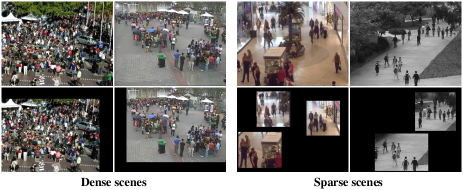
The goal of crowd counting is to count the number of crowds in a surveillance scene, which lays on an important component in many computer vision applications. As the first and the most important part of crowd management, automatic crowd counting can monitor the crowd density of surveillance areas and alert the manager for safety control if the density exceeds specified thresholds. However, precise crowd estimation remains challenging as it demands the extractor to be able to capture pedestrians in various scenes with diverse population distribution (see Figure 1).
Previous methods [1, 2] adopt a detection-style framework, where a sliding window detector is used to estimate the number of people. The limitation of such detection-based methods is that severe occlusion among people in a clustered environment always results in poor performance. To deal with images of dense crowds, some focus on regression-based methods [3, 4], which directly learn a mapping from the features of image patches to the count in the region. Despite the progress in addressing the issues of occlusion, these methods are not efficient since extracting hand-craft features consumes many resources.
In the past decades, the approaches built on Convolutional Neural Networks (CNN) have shown strong generalization ability to handle complicated scenarios by virtue of automatic feature extraction process. However, the performance of different models varies largely across different crowd densities. MCNN [5], utilizing three simple columns with different receptive fields to tackle the scale variations, performs well in sparsely populated scenes such as UCSD dataset but loses its superiority in dense crowd scenes like Shanghai dataset. Whereas SaCNN [6] that incorporates a deep backbone with small fixed kernels turns out to be the opposite. This indicates that a single model is not sufficient enough to effectively cope with all datasets with multiple density levels. Even for images in the same dataset, the distribution of crowds is not uniform, which means processing the whole image with one fixed model usually results in under-estimating or over-estimating count in the crowd image. The work Switch-CNN [7] divides the crowd scenes into non-overlapping patches and sends each patch to a particular column depending on the classification network. Although this strategy improves the adaptability of the model to some extent, there are two main drawbacks in this work. One is that the representation ability is similar for each column with the same capacity, the other is that artificially dividing images is not proper.
One obvious solution to address these problems is to assign adaptive capacities to different portions across the scene based on their density levels. The aforementioned examples illustrate that a deep network is able to handle the regions with high density while a shallow network achieves better performance in sparse regions. Therefore, the goal is divided into two aspects: (1) a model is built to automatically distinguish areas of different density levels in the scene, as is shown in Figure 1; (2) networks of different capacities are specialized for specific areas and integrated to obtain the final result.
To achieve this, we propose the Adaptive Capacity Multi-scale CNNs (ACM-CNN), which could focus on important regions via count attention mechanism without prior knowledge and assign its capacity depending on the density level. This is achieved by exploiting three subnetworks: a coarse network, fine network and smooth network. The coarse network is a multi-column architecture with shallow layers, which is used to locate dense regions and generate a rough feature map. While the fine network, a deep architecture based on VGGNets [8], processes the dense regions into a fine feature map. Since adding up two feature maps directly will lead to the sense of division in the result images, we incorporate the smooth network to fuse two features organically and thereby generate the high-quality density map. ACM-CNN is a fully convolutional design which can be optimized via an end-to-end training scheme.
In summary, the main contributions of this paper are:
-
1.
As far as we know, our work is the first attempt to introduce the adaptive capacity model for crowd counting problem. The primary aim is to take advantage of the different complex networks, which have unique representation abilities to deal with the regions with different density levels.
-
2.
We propose a novel attention mechanism termed as count attention, which could automatically locate dense regions of the input without prior knowledge.
-
3.
We propose a general crowd counting system that can choose the proper network of the right capacity for a specific scene of crowd distribution.
2 Related work
2.1 Crowd counting
Crowd counting has attracted lots of researchers to create various methods in pursuit of a more accurate result [9, 10, 11, 12, 13]. The earlier traditional methods [2] which adopt a detection-style framework have trouble with solving severe occlusions and high clutter. To overcome this issue, regression-based methods [3, 4] have been introduced. The main idea of these methods is to learn a mapping between features extracted from the local images to their counts. Nevertheless, the representation ability of the low-level features are limited, which cannot be widely applied. Recently, most researchers focus on Convolutional Neural Network (CNN) based approaches inspired by the great success in visual classification and recognition [14, 15, 16]. In order to cope with the scale variation of people in crowd counting, the MCNN [5] use receptive fields of different sizes in each column to capture a specific range of head sizes. With similar idea, Sam et al. [7] train a switch classifier to choose the best column for image patches while Sindagi et al. [17] encode local and global context into the density estimation process to boost the performance. Further, Sam et al. [18] extend their previous work by training a growing CNN which can progressively increase its capacity. Later, scale aggregation modules are proposed by Cao et al. [19] to improve the representation ability and scale diversity of features. Instead of using multi-column architectures, Li et al. [20] modify the VGG nets with dilated convolutional filters to aggregate the multi-scale contextual information. Liu et al. [21] adaptively adopt detection and regression count estimations based on the density conditions. Differently, some works pay more attention to context information. Ranjan et al. [22] propose an iterative crowd counting framework, which first produces the low-resolution density map and then uses it to further generate the high-resolution density map. Further, multi-scale contextual information is incorporated into an end-to-end trainable pipeline CAN [23], so the proposed network is capable of exploiting the right context at each image location.
2.2 Attention mechanism
Recent years have witnessed the boom of deep convolutional nerual network in many challenging tasks, ranging from image classification to object detection [24, 25, 26, 27, 28]. However, it is computationally expensive because the amount of the computation scales increases linearly with the number of image pixels. In parallel, the concept of attention has gained popularity recently in training neural networks, allowing models to learn alignments between different modalities [29, 30]. In [31], researchers attempt to use hard attention mechanism learning to selectively focus on task-relevant input regions, thus improving the accuracy of recognizing multiple objects and the efficiency of computation. Almahairi et al. [32] propose dynamic capacity network based on hard attention mechanism that efficiently identifies input regions to which the DCN s output is most sensitive and we should devote more capacity. Recently, some researchers attempt to use the attention mechanism in crowd counting. MA Hossain et al. [33] propose a novel scale-aware attention network by combining both global and local scale attentions. In addition, a novel dual path multi-scale fusion network architecture with attention mechanism named SFANet [34] is proposed, which can perform accurate count estimation for highly congested crowd scenes. Inspired by these works above, we prove that it is effective to introduce the attention mechanism in crowd counting because networks with different complexity have their unique characterization capabilities for different population density regions. Therefore, we propose a new attention strategy named count attention that assigns different capacities to different portions of the input.
3 Methodology
3.1 Count Attention
As discussed in Introduction, different types of networks have their specific learning ability in areas with different crowd density, hence our primary task is to differentiate regions of various density levels. In order to introduce the attention strategy, we must first describe how to conduct the data processing, which is converting an image with labeled people heads to a density map.
Suppose the head at pixel , it can be represented as a delta function . Therefore, we can formulate the image with labeled head positions as:
| (1) |
Due to the fact that the cameras are generally not in a bird-view, the pixels associated with different locations correspond to different scales. Therefore, we should take the perspective distortion into consideration. Following the method introduced in the MCNN [5], the geometry-adaptive kernels are applied to generate the density maps. Specifically, the ground truth is computed by blurring each head annotation with a Gaussian kernel normalized to one, which is:
| (2) |
where is denoted as the average distance between the head and its nearest neighbors, and are hyper-parameters. In this paper, we set = 0.3 and = 3. Thus, the variance of Gaussian kernel is in proportion to . When the crowd density is larger, will be smaller. Accordingly, will be smaller. For one head, the integration of density values equals to one, so the smaller means larger center value. In conclusion, the highest values in the map indicate the most densely populated area to which the network should pay great attention. The count attention mechanism is to traverse all the pixels in the density map to select a set of positions with highest pixel values and crop a series of blocks centering on these points as the attention regions (dense crowd regions).
3.2 Adaptive Capacity Multi-scale CNN
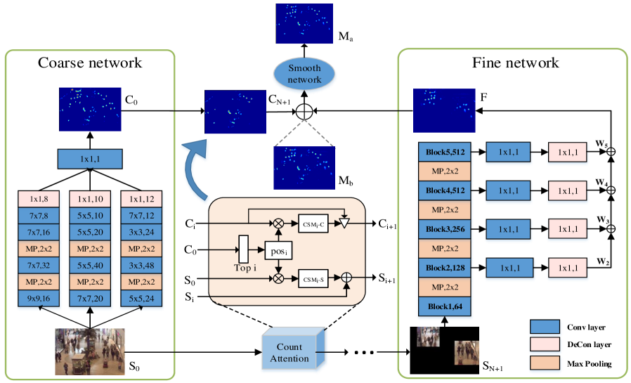
Our model is composed of a coarse network, fine network, and smooth network as shown in Figure 2. Given an input image , the coarse network first extracts its abstract features to generate a rough density map . To further boost the quality of the density map , count attention is applied to iteratively generate specific high-density level regions . In detail, through this strategy, the geometric locations of () highest pixel in are picked as a mapping center at each time, denoted as . Similarly, the corresponding spatial mapping region centering on is represented as . We generate a blank image with the same size as and use () to represent a high-density area map generated by each iteration. Apparently, when equals 1, indicate the initialized blank map . In each iteration, the of input image () fills in , which is formulated as:
| (3) |
Here means cropping the region of according to the corresponding spatial mapping region centering on . Then this process keeps loop until equals . The whole procedure can be represented as:
| (4) |
In this way, the high-density regions are selected and then relayed to a fine network to capture high-level abstraction F. To incorporate initial map with F, the low-density regions of are required to be preserved while the remaining area needs to be discarded. This step can also be synchronized with the aforementioned count attention. We use () to represent the left density map after each iteration. When equals 1, we define is identical with . In each iteration, the of feature map () is gradually stripped out from a feature map , which is formulated as:
| (5) |
Then this process keeps loop until equals . The whole procedure can also be represented as:
| (6) |
After obtaining low-density feature , it can add up with to obtain a more accurate feature map . However, this fusion map still exposes a sense of stiff merging. To solve this issue, this fusion result is relayed to a smooth network containing several convolutional layers to produce the final density map .
The detailed design of coarse network, fine network, and smooth network will be introduced in the following section.
3.3 Model Configuration
Coarse network A three-column CNN which is similar
to MCNN [5] for identical kernel size and filter
number constitutes the coarse network. However, prominent difference
resides in the deconvolution layer following each column of the
network, which up-samples to generate the feature map with the same
size as the input image, as is shown in Figure 2
pink rectangle. Compared to the down-sampling resultant map of MCNN
[5], the deconvolution layer can ensure more
accurate positions of highest pixel values which are then picked out
as the centers of the selected high-density regions via count
attention mechanism. The coarse network is adopted for the reason of
its simplicity and effectiveness on sparse scenes.
Fine
network The fine network is based on VGG-16 with all the fully
connected layers and the last pooling layer removed. Four 1*1
convolution layers followed by 1*1 deconvolution layers are
connected to the last four blocks ( ()) respectively to deliver the different levels of
semantic information. Suppose () represents
the output of each deconvolution layer. In order to effectively
integrate these context, four learnable weights () are assigned to () respectively
for dynamically adjusting the importance of each component, which
can be formulated as:
| (7) |
Where represents the fine feature map. This strategy helps to
achieve more fine granularity crowd description. Similarly, the
choice of this fine network relies largely on its superiority
dealing with dense scenes.
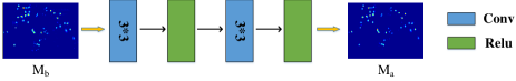
Smooth network The smooth
network is made up of CR(12,3) and CR(1,3), where C means
convolution layer, R refers to ReLU layer, the first number in every
brace indicates filter number, and the second number denotes filter
size. An overview of the mooth network is shown in Figure
3. The use of this smooth network contributes to smoother
prediction map generation.
3.4 Networks Optimization
The whole model is trained on the entire dataset by back-propagating loss via an end-to-end strategy. The design of our model ensures that all the desired results have the same resolutions as the input images. Suppose there are training images and the parameters before the smooth network are . Then represents the merged feature map before the smooth network for the i-th input image . We first conduct a supervision of this intermediate result to ensure priority learning of the coarse network and the fine network. That is:
| (8) |
where indicates the corresponding ground truth for . Besides, the differences between the final density map and the ground truth are minimized by:
| (9) |
where indicates the parameters of the smooth network. A weighted combination is computed on the above two loss functions to get the final objective:
| (10) |
where is the hyper-parameter balancing the learning of the first two networks and the smooth network. In our experiments, the value is set to 1. We train the proposed model using the Adam solver with the following parameters: learning rate and batch size .
4 Experiments
4.1 Evaluation Metrics
The proposed model ACM-CNN is evaluated on four major crowd counting datasets. Following the existing works, we adopt two standard metrics, Mean Absolute Error (MAE) and Mean Squared Error (MSE), to benchmark the model. For a test sequence with images, MAE and MSE are defined as follows:
| (11) |
| (12) |
where indicates the actual count and represents the estimated number of pedestrians in the i-th image. MAE reflects the accuracy of the predicted count and MSE is an indicator of the robustness.
| Part_A | Part_B | |||
|---|---|---|---|---|
| Method | MAE | MSE | MAE | MSE |
| Zhang et al. (2015) | 181.8 | 277.7 | 32.0 | 49.8 |
| MCNN (2016) | 110.2 | 173.2 | 26.4 | 41.3 |
| TDF-CNN | 97.5 | 145.1 | 20.7 | 32.8 |
| Switching-CNN | 90.4 | 135.0 | 21.6 | 33.4 |
| CP-CNN | 73.6 | 106.4 | 20.1 | 30.1 |
| SaCNN | 86.8 | 139.2 | 16.2 | 25.8 |
| ACM-CNN (ours) | 72.2 | 103.5 | 17.5 | 22.7 |
4.2 Shanghaitech dataset
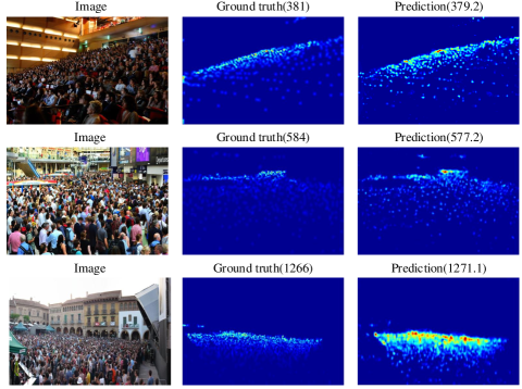
The Shanghaitech crowd counting dataset [5] consists of 1198 annotated images with a total of 330,165 people, which is said to be the largest one in terms of the number of annotated people. It has two parts: one of the parts named Part_A contains 482 images which are randomly crawled from the Internet, the other named Part_B includes 716 images which are taken from the busy streets of metropolitan area in Shanghai. Each of the two parts is divided into training and testing sets: in Part_A, 300 images are used for training and the remaining are used for testing while 400 images of Part_B are used for training and 316 for testing. To augment the training set, we crop 100 patches from each image at random locations and each patch is 1/4 size of the original image for both Part_A and Part_B. We compare performance between our approach with other state-of-the-art methods in Table 1, including Zhang et al. [35], MCNN [5], TDF-CNN [36], Switch-CNN [7], CP-CNN [17], SaCNN [6]. The results indicate that ACM-CNN is able to calculate the number of crowds more accurately. We also report some samples of the test cases in Figure 4.
| Method | Scene1 | Scene2 | Scene3 | Scene4 | Scene5 | Average MAE |
| LBP + RR [5] | 13.6 | 59.8 | 37.1 | 21.8 | 23.4 | 31.0 |
| Zhang et al.[35] | 9.8 | 14.1 | 14.3 | 22.2 | 3.7 | 12.9 |
| MCNN [5] | 3.4 | 20.6 | 12.9 | 13.0 | 8.1 | 11.6 |
| Switching-CNN [7] | 4.4 | 15.7 | 10.0 | 11.0 | 5.9 | 9.4 |
| CP-CNN [17] | 2.9 | 14.7 | 10.5 | 10.4 | 5.8 | 8.86 |
| DecideNet [21] | 2.00 | 13.14 | 8.90 | 17.40 | 4.75 | 9.23 |
| ACM-CNN (ours) | 2.4 | 10.4 | 11.4 | 15.6 | 3.0 | 8.56 |
4.3 WorldExpo’10 dataset
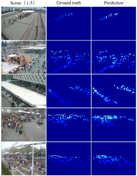
The WorldExpo 10 dataset introduced by [35] consists of 1132 annotated video sequences that cover a large variety of scenes captured by 108 surveillance equipment in Shanghai 2010 WorldEXPO. Each frame of one sequence with 50fps frame rate has a regular 576 x 720 pixels. A total of 199,923 pedestrians are labeled at the centers of their heads in 3980 frames. They also provide ROI for each of the scenes. We split the frames into two parts: one part with 3380 frames in 103 scenes are treated as training and verification sets, and the other part with 600 frames in 5 scenes are treated as test sets. In order to conduct data augmentation, we crop 10 patches of size 256*256 per image, and the same operation is done on the ROI (regions of interest) images. We compare the performance of our model with other state-of-the-art methods and the results are reported in Table 2. Also, we visualize the results of the five test scenes in Figure 5.
| Method | MAE | MSE |
|---|---|---|
| Gaussian Process Regression | 2.16 | 7.45 |
| Zhang et al. (2015) | 1.60 | 3.31 |
| MCNN (2016) | 1.07 | 1.35 |
| Switching-CNN | 1.62 | 2.10 |
| CSRNet | 1.16 | 1.47 |
| ACM-CNN (ours) | 1.01 | 1.29 |
4.4 UCSD dataset
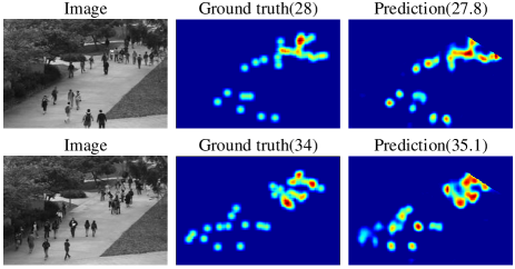
Our second experiment concentrates on crowd counting for UCSD dataset introduced in [37]. It is acquired with a stationary camera mounted at an elevation in UCSD campus. The crowd density ranges from sparse to very crowded. This is a 2000-frame video dataset that is recorded at 10 fps with a frame size of 158 *238. Different from Shanghaitech dataset above, this dataset not only provides ground truth with figure coordinates but also region of interest (ROI) for each frame. Of the 2000 frames, we send frames 601 through 1400 into the model for training while the remaining frames are used for testing. There is no process of augmentation due to the similarity of pictures. During training, we separately prune the ground truth, merged map, and the final map with ROI. As a result, the error is back-propagated for areas inside the ROI. Table 3 lists the results of all methods and our approach is able to offer better MAE and MSE in all scenes, which means our model can generate a more accurate density map whether in dense or sparse scenes. Two examples are shown in Figure 6.
| Method | MAE | MSE |
|---|---|---|
| Gaussian process regression | 3.72 | 20.1 |
| Ridge regression | 3.59 | 19.0 |
| MoCNN | 2.75 | 13.4 |
| Count forest | 2.5 | 10.0 |
| ACM-CNN (ours) | 2.3 | 3.1 |
4.5 Mall dataset
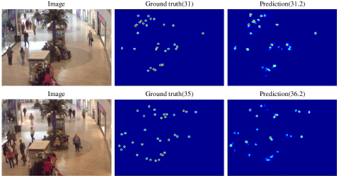
The Mall dataset [4] is captured in a shopping mall using a publicly accessible surveillance camera, which suffers from more challenging lighting conditions and glass surface reflections. It consists of scenes with more diverse crowd densities from sparse to crowd, as well as different activity patterns under different illumination conditions during the day. The video sequence in the dataset is made up of 2000 frames of resolution 320*240 with 6000 instances of labeled pedestrians. Following the existing methods, we use the first 800 frames for training and the remaining 1200 frames for evaluation. During testing, MAE is only computed for regions inside ROI. We perform comparison against Gaussian process regression [37], Ridge regression [4], MoCNN [38], Count forest [39], and achieves state-of-the-art performance shown in Table 4. Examples are presented in Figure 7.
4.6 UCF_CC_50 dataset
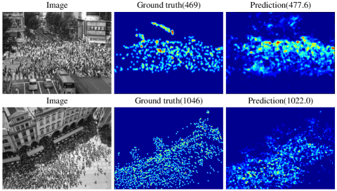
The UCF_CC_50 dataset [40] includes 50 images with a wide range of densities and diverse scenes. This dataset is very challenging for the small size and the large variation in crowd count. As there is no separate test set, a 5-fold cross-validation method is defined for training and testing to verify the performance of the model. We compare the proposed model with Multi-source multi-scale [40], MCNN [5], Switch-CNN [7], CP-CNN [17], SaCNN [6] and our model achieves the best MAE over existing methods, shown in Table 5. Figure 8 shows the generated density maps by our ACM-CNN.
| Method | MAE | MSE |
|---|---|---|
| Multi-source multi-scale | 468.0 | 590.3 |
| MCNN | 377.6 | 509.1 |
| Switch-CNN | 318.1 | 439.2 |
| CP-CNN | 295.8 | 320.9 |
| SaCNN | 314.9 | 424.8 |
| ACM-CNN (ours) | 291.6 | 337 |
5 Analysis
5.1 Parameter Settings
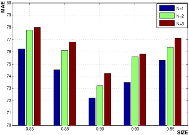
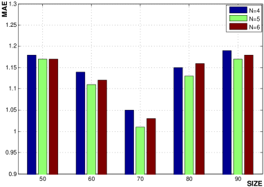
We first empirically study the configuration of the number of attention pixels N and the size of the corresponding patch S, as is shown in Figure 9. Due to the huge diversity in density levels, there are no set of parameters to meet the requirements of balancing the performance of all datasets. Thus, we divide the situation into two types: dense datasets in which all areas of each image are densely populated and sparse datasets where only a small portion of each image are occupied by crowds. As is shown in Table 6, we set a threshold T = 40. When the average crowd count of one dataset exceeds T, it will be classified as a dense dataset, otherwise a sparse dataset. Comparative experiments are respectively performed on two types of representative datasets: Shanghaitech Part_A dataset (dense) and UCSD dataset (sparse). In Figure 9(a), the size represents the ratio of the patch size to the original image’s height and width, whereas in Figure 9(b), the size indicates the true pixel value. This is because images in UCSD dataset share the same size but Shanghaitech dataset doesn’t conform to the condition. According to the final results, we set N=1 and S= [0.9*height,0.9*width] for Shanghai Part_A dataset, N=5 and S = [70,70] ([0.4*height,0.3*width]) for UCSD datasets. The parameters settings of five datasets used in this paper are listed in Table 7.
| Dataset | Max | Min | Ave | |
|---|---|---|---|---|
| Shanghaitech | Part_A | 3139 | 33 | 501.4 |
| Part_B | 578 | 9 | 123.6 | |
| WorldExpo’10 | 253 | 1 | 50.2 | |
| UCSD | 46 | 11 | 24.9 | |
| Mall | 53 | 13 | 31.7 | |
| UCF_CC_50 | 4543 | 94 | 1279.5 | |
| Type | Datasets | Configure | |||
|---|---|---|---|---|---|
| Dense |
|
N=1 S=[0.9*height,0.9*width] | |||
| Sparse |
|
N=5 S=[0.4*height,0.3*width] |
5.2 Algorithmic Study
| Method | Shanghaitech | UCSD | ||
|---|---|---|---|---|
| MAE | MSE | MAE | MSE | |
| C | 106.2 | 168.4 | 1.60 | 2.30 |
| F | 80.9 | 128.1 | 2.30 | 3.50 |
| C+F | 74.5 | 108.2 | 1.19 | 1.60 |
| C+F+S | 72.2 | 103.5 | 1.01 | 1.29 |
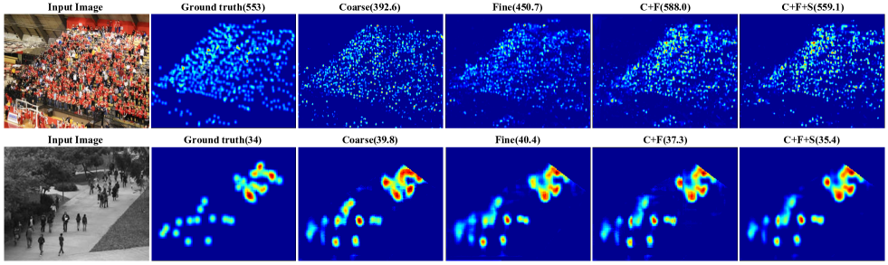
In this section, we study the effectiveness of modules in the proposed ACM-CNN and count attention mechanism on the final accuracy. All ablations are performed on Part_A of Shanghaitech and UCSD dataset as they represent two types of datasets: dense and sparse. First, the first two rows in Table 8 list the performance of only coarse network (denoted as C) or only fine network (denoted as F) on two datasets, which further validate the previous standpoint that a deep network is suitable for dense scenes while a shallow network performs better in sparse scenes. In order to demonstrate the effect of count attention mechanism, we combine the coarse network and the fine network via this strategy (denoted as C+F). It is obvious that there is a significant improvement on two datasets for such a combination compared to using any one of the modules separately. When introducing the smooth network (defined as C+F+S), the estimation error is further reduced. This means that the smooth network is not only able to alleviate the sense of fragmentation in the result, but also capable of improving the model accuracy. Figure 10 shows the density maps predicted by various networks in Table 8 along with their corresponding ground truths. We can see that the coarse network yields density maps with fine-grained distribution and the fine networks are more eager to achieve overall accuracy. Besides, there is indeed a clear division in the results generated by the integration of two networks, and the introduction of the smooth network resolves the problem to some extent.
5.3 Model generality
The proposed model is a general framework which means that the effectiveness of the algorithm does not depend on the choice of sub-networks. To verify this generality, we train a variant of our model using the modules introduced in CrowdNet [41]. Specifically, the deep network and shallow network in CrowdNet serve as the fine network and the coarse network in our model respectively. Without the smooth network, we perform the experiments on the UCSD datasets and the results are listed in Table 9.
| Method | MAE | MSE |
|---|---|---|
| Shallow Network | 1.7 | 2.1 |
| Deep Network | 2.2 | 2.9 |
| Deep + Shallow (CrowdNet contact) | 1.5 | 1.7 |
| Deep + Shallow (Count attention) | 1.2 | 1.4 |
CrowdNet concatenates the predictions from the deep and shallow networks to produce the final density map. From the table, we can see that it is more effective than using any of these networks alone. However, combining the two networks with our attention mechanism is able to achieve better performance, which expresses the generality of our model. In conclusion, our whole structure is not limited to the choice of sub-networks. It is a general crowd counting system to greatly improve the accuracy of predictions.
6 Conclusion
In this paper, we propose the Adaptive Multi-scale convolutional networks, which can assign different capacities to different portions of the input and characterize them with corresponding networks. Our model consists of three modules, including the coarse network, the fine network and the smooth network. It can be regarded as a general crowd counting system since the choice of three types of sub-networks is flexible. Extensive experiments on five representative datasets (three dense datasets and two sparse datasets) demonstrate that the proposed model delivers state-of-the-art performance over existing methods. Further, we validate the effectiveness of modules and the attention mechanism with ablations. In the future, we would like to consider extending our method to fit for other scenario [42, 43].
References
References
- [1] P. Viola, M. J. Jones, D. Snow, Detecting pedestrians using patterns of motion and appearance, in: null, IEEE, 2003, p. 734.
- [2] Y. P. Kocak, S. Sevgen, Detecting and counting people using real-time directional algorithms implemented by compute unified device architecture, Neurocomputing 248 (2017) 105 – 111, neural Networks : Learning Algorithms and Classification Systems.
- [3] A. B. Chan, N. Vasconcelos, Bayesian poisson regression for crowd counting, in: Computer Vision, 2009 IEEE 12th International Conference on, IEEE, 2009, pp. 545–551.
- [4] K. Chen, C. C. Loy, S. Gong, T. Xiang, Feature mining for localised crowd counting., in: BMVC, Vol. 1, 2012, p. 3.
- [5] Y. Zhang, D. Zhou, S. Chen, S. Gao, Y. Ma, Single-image crowd counting via multi-column convolutional neural network, in: Proceedings of the IEEE Conference on Computer Vision and Pattern Recognition, 2016, pp. 589–597.
- [6] L. Zhang, M. Shi, Q. Chen, Crowd counting via scale-adaptive convolutional neural network, CoRR abs/1711.04433.
- [7] D. B. Sam, S. Surya, R. V. Babu, Switching convolutional neural network for crowd counting, in: Proceedings of the IEEE Conference on Computer Vision and Pattern Recognition, Vol. 1, 2017, p. 6.
- [8] K. Simonyan, A. Zisserman, Very deep convolutional networks for large-scale image recognition, CoRR abs/1409.1556.
- [9] Q. Wang, J. Gao, W. Lin, Y. Yuan, Learning from synthetic data for crowd counting in the wild, CoRR abs/1903.03303.
- [10] Q. Wang, M. Chen, F. Nie, X. Li, Detecting coherent groups in crowd scenes by multiview clustering, IEEE Transactions on Pattern Analysis and Machine Intelligence (2018) 1–1doi:10.1109/TPAMI.2018.2875002.
- [11] Q. Wang, J. Wan, Y. Yuan, Deep metric learning for crowdedness regression, IEEE Transactions on Circuits and Systems for Video Technology 28 (10) (2018) 2633–2643. doi:10.1109/TCSVT.2017.2703920.
- [12] Y. Zhang, C. Zhou, F. Chang, A. C. Kot, Multi-resolution attention convolutional neural network for crowd counting, Neurocomputing 329 (2019) 144 – 152. doi:https://doi.org/10.1016/j.neucom.2018.10.058.
- [13] V. A. Sindagi, V. M. Patel, A survey of recent advances in cnn-based single image crowd counting and density estimation, Pattern Recognition Letters 107 (2018) 3 – 16, video Surveillance-oriented Biometrics. doi:https://doi.org/10.1016/j.patrec.2017.07.007.
- [14] X. Jiang, Z. Xiao, B. Zhang, X. Zhen, X. Cao, D. S. Doermann, L. Shao, Crowd counting and density estimation by trellis encoder-decoder network, CoRR abs/1903.00853.
- [15] N. Liu, Y. Long, C. Zou, Q. Niu, L. Pan, H. Wu, Adcrowdnet: An attention-injective deformable convolutional network for crowd understanding, CoRR abs/1811.11968.
- [16] Y. Liu, M. Shi, Q. Zhao, X. Wang, Point in, box out: Beyond counting persons in crowds, CoRR abs/1904.01333.
- [17] V. A. Sindagi, V. M. Patel, Generating high-quality crowd density maps using contextual pyramid cnns, in: The IEEE International Conference on Computer Vision (ICCV), 2017.
- [18] D. Babu Sam, N. N. Sajjan, R. Venkatesh Babu, M. Srinivasan, Divide and grow: Capturing huge diversity in crowd images with incrementally growing cnn, in: The IEEE Conference on Computer Vision and Pattern Recognition (CVPR), 2018.
- [19] X. Cao, Z. Wang, Y. Zhao, F. Su, Scale aggregation network for accurate and efficient crowd counting, in: The European Conference on Computer Vision (ECCV), 2018.
- [20] Y. Li, X. Zhang, D. Chen, Csrnet: Dilated convolutional neural networks for understanding the highly congested scenes, in: The IEEE Conference on Computer Vision and Pattern Recognition (CVPR), 2018.
- [21] J. Liu, C. Gao, D. Meng, A. G. Hauptmann, Decidenet: Counting varying density crowds through attention guided detection and density estimation, in: The IEEE Conference on Computer Vision and Pattern Recognition (CVPR), 2018.
- [22] V. Ranjan, H. Le, M. Hoai, Iterative crowd counting, in: The European Conference on Computer Vision (ECCV), 2018.
- [23] W. Liu, M. Salzmann, P. Fua, Context-aware crowd counting, CoRR abs/1811.10452.
- [24] L.-C. Chen, G. Papandreou, I. Kokkinos, K. Murphy, A. L. Yuille, Deeplab: Semantic image segmentation with deep convolutional nets, atrous convolution, and fully connected crfs, arXiv preprint arXiv:1606.00915.
- [25] S. S. Kruthiventi, K. Ayush, R. V. Babu, Deepfix: A fully convolutional neural network for predicting human eye fixations, IEEE Transactions on Image Processing.
- [26] Y. Ji, H. Zhang, Q. J. Wu, Salient object detection via multi-scale attention cnn, Neurocomputing 322 (2018) 130 – 140.
- [27] A. R. Gepperth, M. G. Ortiz, E. Sattarov, B. Heisele, Dynamic attention priors: a new and efficient concept for improving object detection, Neurocomputing 197 (2016) 14 – 28.
- [28] K. G. Y. Y. S. C. Shuangjie Xu, Yu Cheng, P. Zhou, Jointly attentive spatial-temporal pooling networks for video-based person re-identification, in: ICCV, 2017.
-
[29]
V. Mnih, N. Heess, A. Graves, K. Kavukcuoglu,
Recurrent models of visual attention,
CoRR abs/1406.6247.
URL http://arxiv.org/abs/1406.6247 - [30] Z. Gan, Y. Cheng, A. E. Kholy, L. Li, J. Liu, J. Gao, Multi-step reasoning via recurrent dual attention for visual dialog, in: Proceedings of the 57th Conference of the Association for Computational Linguistics, ACL 2019, Florence, Italy, July 28- August 2, 2019, Volume 1: Long Papers, 2019, pp. 6463–6474.
-
[31]
J. Ba, V. Mnih, K. Kavukcuoglu, Multiple
object recognition with visual attention, CoRR abs/1412.7755.
URL http://arxiv.org/abs/1412.7755 - [32] A. Almahairi, N. Ballas, T. Cooijmans, Y. Zheng, H. Larochelle, A. C. Courville, Dynamic capacity networks, CoRR abs/1511.07838.
- [33] M. Hossain, M. Hosseinzadeh, O. Chanda, Y. Wang, Crowd counting using scale-aware attention networks, in: 2019 IEEE Winter Conference on Applications of Computer Vision (WACV), 2019, pp. 1280–1288. doi:10.1109/WACV.2019.00141.
- [34] L. Zhu, Z. Zhao, C. Lu, Y. Lin, Y. Peng, T. Yao, Dual path multi-scale fusion networks with attention for crowd counting, CoRR abs/1902.01115.
- [35] C. Zhang, H. Li, X. Wang, X. Yang, Cross-scene crowd counting via deep convolutional neural networks, in: Proceedings of the IEEE Conference on Computer Vision and Pattern Recognition, 2015, pp. 833–841.
- [36] D. B. Sam, R. V. Babu, Top-down feedback for crowd counting convolutional neural network, CoRR abs/1807.08881.
- [37] A. B. Chan, Z.-S. J. Liang, N. Vasconcelos, Privacy preserving crowd monitoring: Counting people without people models or tracking, in: Computer Vision and Pattern Recognition, 2008. CVPR 2008. IEEE Conference on, IEEE, 2008, pp. 1–7.
- [38] S. Kumagai, K. Hotta, T. Kurita, Mixture of counting cnns: Adaptive integration of cnns specialized to specific appearance for crowd counting, CoRR abs/1703.09393.
- [39] V. Q. Pham, T. Kozakaya, O. Yamaguchi, R. Okada, Count forest: Co-voting uncertain number of targets using random forest for crowd density estimation, in: IEEE International Conference on Computer Vision, 2015, pp. 3253–3261.
- [40] H. Idrees, I. Saleemi, C. Seibert, M. Shah, Multi-source multi-scale counting in extremely dense crowd images, in: The IEEE Conference on Computer Vision and Pattern Recognition (CVPR), 2013.
- [41] L. Boominathan, S. S. S. Kruthiventi, R. V. Babu, Crowdnet: A deep convolutional network for dense crowd counting, in: Proceedings of the 2016 ACM on Multimedia Conference, MM ’16, ACM, New York, NY, USA, 2016, pp. 640–644.
- [42] Y. Cheng, Q. Fan, S. Pankanti, A. Choudhary, Temporal sequence modeling for video event detection, in: Proceedings of the 2014 IEEE Conference on Computer Vision and Pattern Recognition, CVPR ’14, 2014, pp. 2235–2242.
- [43] J. Wang, Y. Cheng, R. Schmidt Feris, Walk and learn: Facial attribute representation learning from egocentric video and contextual data, in: The IEEE Conference on Computer Vision and Pattern Recognition (CVPR), 2016.